Approximating a flexible beam model in the Loewner framework \shortdate
Approximating a flexible beam model in the Loewner framework
Abstract
The paper develops the Loewner approach for data-based modeling of a linear distributed-parameter system. This approach is applied to a controlled flexible beam model coupled with a spring-mass system. The original dynamical system is described by the Euler-Bernoulli partial differential equation with the interface conditions due to the oscillations of the lumped part. The transfer function of this model is computed analytically, and its sampled values are then used for the data-driven design of a reduced model. A family of approximate realizations of the corresponding input-output map is constructed within the Loewner framework. It is shown that the proposed finite-dimensional approximations are able to capture the key properties of the original dynamics over a given range of observed frequencies. The robustness of the method to noisy data is also investigated.
keywords
Data-driven modeling, flexible structure, Euler–Bernoulli beam, distributed parameter systems, Loewner framework, linear systems, model reduction, noisy data, input-output map, transfer function.1 Introduction
Model reduction techniques can be employed to replace a large-scale system with a complex structure (characterized by multidimensional systems of ordinary differential equations and/or partial differential equations), with a much simpler and smaller dynamical system (characterized by few equations with well-understood dynamics). In the last decades, there have been many methodologies proposed in this direction; we refer the reader to [2, 32, 24, 9, 3] for more details.
A viable alternative to using classical model reduction approaches based on single or double-sided projections (that usually require explicit access to a large-scale model) is to use instead data-driven methods. These latter do not require explicit access to the large-scale model’s structure or matrices. We mention here the Loewner framework (LF) [27], Vector fitting (VF) [19], or the AAA algorithm [28]. When using these, low-order models can be constructed directly from data in the frequency domain (samples of the transfer function). Such methods can be viewed as rational approximation tools by means of interpolation (LF), least-squares fit (VF), or a mixed approach (AAA). Other data-driven methods that has emerged in recent years are dynamic mode decomposition (DMD) and operator inference (OpInf), which use time-domain snapshots of the state variables and then fit a particular structured model by computing the appropriate matrices (in reduced coordinates). Details on DMD can be found in [24], while details on OpInf can be found in [29, 6].
We consider here the problem of data-driven rational approximation by means of fitting a linear time-invariant (LTI) dynamical system to a set of measurements (in the frequency domain). The fitted LTI system is characterized in the state-space by the following equations:
| (1) |
where is the input, is the output, is the state vector, and the system matrices are . The transfer function of (1) is given by . We refer to [2] for more details on various methodologies especially tailored to the reduction of linear systems. In recent years, such methods for linear systems have been steadily extended to particular classes of structured linear systems [5, 30], or even to nonlinear structured systems in [16] (without preservation of structure) or in [7] (with preservation of structure). The structures treated include distributed parameters, delay terms or integro-differential equations. In a data-driven setup, the structure-preserving approach is [33] was proposed. Note that the analytical representations of transfer functions have been obtained only for particular classes of distributed parameter systems. We refer to [11, 1] for surveys of results in this area. In the former tutorial article, the authors provide the derivation of a variety of (irrational) transfer functions for systems described by partial-differential equations. It is also shown that the choice of boundary conditions have an influence on the dynamics and on the locations of poles and zeros. In most practical situations, it is desirable to approximate the irrational transfer function by a rational one, for the purpose of controller design.
The Loewner framework approach was shown to be extremely powerful in data-based control problems for wide classes of finite-dimensional control systems, whose transfer functions are rational [4, 3]. However, the efficiency of the Loewner framework for distributed-parameter systems (characterized by irrational transfer functions) still remains to be verified, and the present paper aims at filling this gap. Preliminary analysis was provided for linear time-delay systems in [34, 26], fractional-order systems in [10], or for control purposes in [17, 31]. A recent overview was provided in [22], including amongst others, rational approximation of the Bessel function, of a hyperbolic sine, and of a vibrating beam model from [11]. Hence, the LF was studied in the context of approximating infinite-dimensional models of vibrating beams (with finite-dimensional ones). However, as far as the authors are aware, this is the first contribution that also takes into account the effects of perturbed data, i.e., under additive Gaussian noise.
2 Vibrating beam with attached mass
Consider the Euler–Bernoulli equation describing the transverse vibrations of a flexible beam of length :
| (2) |
where is the beam deflection at point and time , is the Young’s modulus, is the area moment of inertia of the cross-section, is the mass per unit length of the beam, and is the structural damping coefficient. We denote the derivative with respect to time by a dot, while the prime denotes the spatial derivative (i.e., with respect to ). We assume that a mass-spring system (shaker) is attached to the beam at point , so that equation (2) holds for and , and the interface condition is imposed at :
| (3) |
The beam is hinged at both ends, which is formalized by the boundary conditions
| (4) |
System (2)–(4) is controlled by the force applied to the shaker at and piezo actuators, whose actions are characterized in terms of shape functions , . It is also assumed that piezo sensors are located at the points , , i.e. the system outputs are
| (5) |
3 Computation of the transfer function
Let , , …, be inputs of the control system (2)–(5) with zero initial data, denote the Laplace transform of the inputs and outputs by
and
respectively.
After introducing the Laplace transform of with respect to : , we obtain from (2) the following system of ordinary differential equations for :
| (6) |
with
| (7) |
| (8) |
and the variable is treated as a parameter in (6). The general solution of (6) is represented with the matrix exponential as follows:
| (9) |
where
| (10) | ||||
Formula (9) represents the solutions of (6) in terms of their boundary values and at and , respectively, From the boundary conditions (4), we conclude that
| (11) |
To eliminate the parameters , , , , we exploit the property that is of class together with the interface condition (3). As a result, we get the following linear algebraic system with respect to :
| (12) |
where
| (13) |
and
Thus, the vector-valued function is defined by (9) and (11) with , and the components of are linear combinations of , …, :
| (14) |
where the coefficient matrix can be obtained from (8), (13). Then the function , corresponding to the second -derivative of , is expressed as:
| (15) | ||||
where and because of (14). Thus, at each , the above formulas define as a linear combination of , ,…, :
| (16) |
with the coefficients collected from (15). Recalling that the output of the considered system is given by (5), we summarize the computation of the transfer function in the following lemma.
Lemma 1
3.1 Single-input single-output (SISO) case
Let the system be controlled by the shaker force only and the scalar output signal be available. In this particular case, the scalar transfer function is such that . Lemma 1 implies the following result in the considered SISO case.
Lemma 2
4 The Loewner framework for fitting linear time-invariant systems
In what follows, we provide a brief summary of the LF for fitting linear dynamical systems as in (1), from data. The starting point for LF is having access to measurements corresponding to the transfer function of the underlying dynamical process, which can be inferred in practice by means of experimental or model-based procedures. The data set is given by:
| (19) |
by means of sampling is an analytic function (not necessarily rational) on a particular (complex) grid of points ’s. It is to be noted that data sets with an odd number of measurements can also be accommodated in the LF. The first step is to partition the data set in (19) into two disjoint subsets, as follows:
| (20) | ||||
For simplicity, all points are assumed distinct and also , for all ; extensions to Hermite interpolation were proposed in [27].
A typical approach for splitting the data, commonly used in the LF publications, is the “alternate splitting scheme”, described as follows. The left and right sample nodes (and points) are chosen so that they are interlacing each other. More precisely, for , we can write:
| (21) | ||||
We refer the reader to [22] for a more comprehensive account of data partitioning strategies in the Loewner framework; there, the “half-hal” splitting is mentioned together with approaches that split the data based on the magnitude of the data samples.
The goal is to find a rational function denoted with , such that the following interpolation conditions are (approximately) fulfilled:
| (22) |
In order to accomplish this scope, we first arrange the elements of the original data set , partitioned as in (20) in matrix format. Hence, the Loewner matrix and the shifted Loewner matrix are defined as follows
| (23) |
while the data vectors are given by:
| (24) |
The Loewner model is hence constructed as follows:
The following Sylvester equations are satisfied by the Loewner and shifted Loewner matrices, as shown in [4] (here, ):
| (25) |
where and . The following relations expressing the shifted Loewner matrix to the Loewner matrix, in two distinct ways, hold:
| (26) |
Hence, the explicit computation of large Loewner matrices can be avoided by means of computing (approximated, low-rank) solutions of the Sylvester equations in (25). This can be accomplished, e.g., by means of using optimized and robust numerical tools such as [8].
Provided that enough data are available, the pencil is often singular. For example, if the data in 19 were generated from a rational function corresponding to a minimal LTI system of dimension , i.e., , then this corresponds to the case . Then, in the perfect setup (no noisy data), one would encounter zero singular values when performing the singular value decomposition (SVD) of the pencil , where is chosen to be different than the eigenvalues of matrix . In such cases, an SVD of augmented Loewner matrices is computed, and the dominating part is selected as:
| (27) |
where , , ,, , and denotes the conjugate-transpose of matrix . This is performed in order to find projection matrices , as described in [4]. Here, represents the truncation index. Then, the system matrices corresponding to a projected Loewner model of dimension can be computed using the truncated singular vector matrices and :
| (28) | ||||
and therefore, directly finds a state-space realization corresponding to the reduced-order system of equations
| (29) |
The transfer function of the reduced Loewner model in (29) is written as , and it provides a good approximant to the original transfer function . Then, may be expanded in a pole/zero or pole/residue format. These values represent system invariants and can be related to the inherent dynamics. It is noted that the state-space realization is not unique, and that is why an extra step is required. More implementation details and properties of the LF procedure can be found in [4, 22].
5 Numerical examples
5.1 Analysis on the unperturbed data
In this section, we present two numerical test cases based on sampling the transfer function explicitly derived in Section 3. We consider the SISO system with the choice of physical parameters (18). Then the scalar transfer function in Lemma 2 is sampled at the purely imaginary grid points , with , which are equally distributed in the range of physical frequencies from to . The data partitioning scheme (into the left and right disjoint subsets) chosen here is the “alternate” one, previously described in Section 4. We also note that complex conjugated data is added to the process to enforce real-valued models; more details on how this is achieved can be found in [4].
Two values of the structural damping parameter in (2) are considered for the numerical simulations: (“large” damping) and (“small” damping). The case is depicted in Figs. 1–4, for which we are fitting a Loewner model of order (with a rational transfer function). Additionally, the case is presented in Figs. 5–8; for this case, we are fitting a Loewner model of order . It should be noted that the Loewner framework does not automatically impose stability; post-processing methods can be applied whenever unstable poles appear, as described in [15].
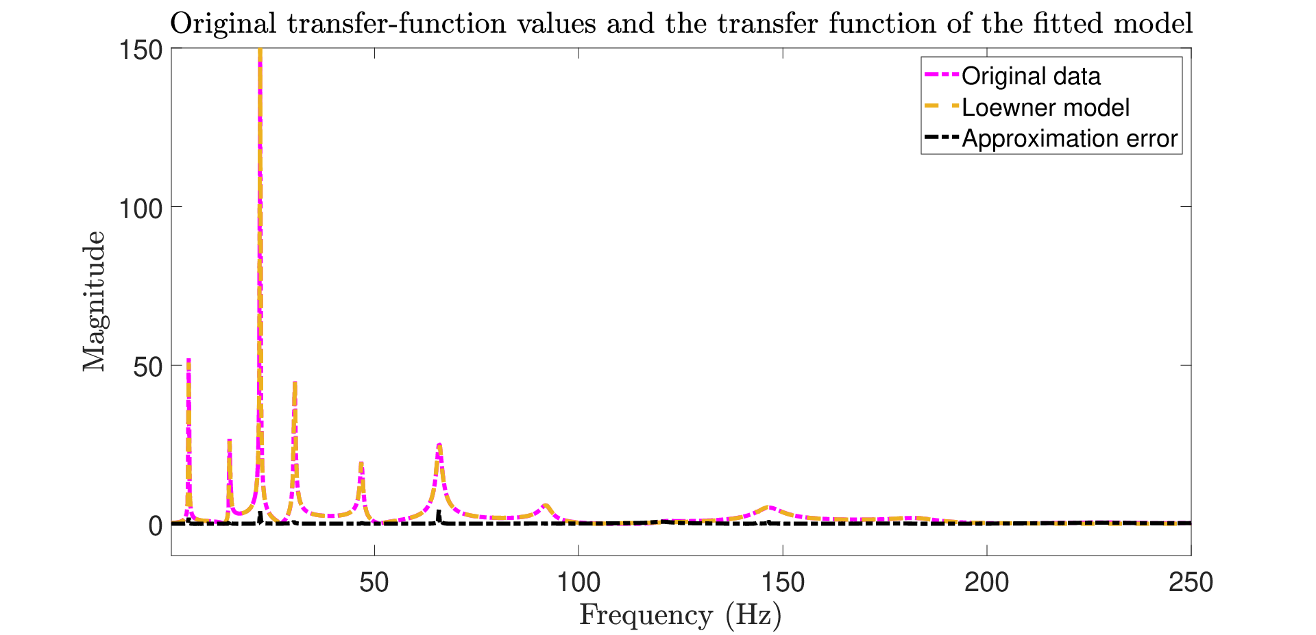
We observe that the Loewner model approximates the original transfer function with good accuracy in the whole range of test frequencies (the approximation error of order in Fig. 3, and of order in Fig. 7). It is also clear that these approximate models preserve the stability property (the maximal real part of in Fig. 4 is , while the maximal real part of in Fig. 8 is ).
Although the transfer function of the considered distributed parameter function is not rational, the decay of singular values associated with the Loewner matrices in Figs. 1 and 5 seems to indicate the opportunity to enforce rational approximation. More precisely, in both cases, a plateau (flat portion of the graph) is observed after a steep decay. In Figs. 1 and 5, we only depict the first singular values (out of , which is the dimension of the Loewner matrices and ). In the first test case, the decay is faster than in the second one. The dimensions of the reduced-order models were chosen in accordance with this phenomenon (i.e. for the first and for the second). However, such a clear and steep decay as seen in Figs. 1 and 5, is seldom noticed in experimental data. In such scenarios, the data can be perturbed, i.e., by means of noise. We treat this case below.


5.2 Analysis on the perturbed data (by means of artificial additive Gaussian noise)
In this subsection, we analyze the robustness of the LF when applied to perturbed (noisy) data. A preliminary analysis of such endeavors was reported in [25, 12, 23] and in [35, 14]. Similarly to the approaches in these publications, we will include additive Gaussian noise into the measurements of the transfer function from Lemma 2. More precisely, for all previous grid points , the new data are, for and :
| (30) |
Here, the “noise power” is chosen so that , while the values and are drawn from the standard normal distribution. For simplicity, we use the term “noise level ” (in the subsequent text and plots). Also, for the sake of brevity, we will restrict our analysis to the case of a smaller damping coefficient: .
The first numerical experiment that is shown here is concerned with the decay of singular values for Loewner matrices under the influence of noise. As previously pointed out in [25, 18], the effect of noise is generally reflected in the “flattening” of the singular value curve. This is especially valid for the “alternate” splitting, and not as much for the “half-half” splitting (as shown in [18]). This is precisely the phenomenon observed in Fig. 9. Additionally, there are a number of dominant singular values that are less prone to perturbations; depending on the noise levels, it is clear that this number decreases with the increase of the noise power. For example, when there are 22 singular values that seem to be stagnant. This is hence another effect of the noise in data for LF; deciding the order of the fitted model becomes a more challenging task, and one needs to be careful to avoid over-fitting.

Next we fix the noise level at and record the poles of the fitted Loewner model on the noisy data. We compare those with the original poles, and the results are depicted in Fig. 10. As expected, most of the (dominant) poles seem to be matching well, with the remark that the noisy data introduces spurious poles.

However, as shown in Fig. 11, the effects of the noise (for this level) do not seem to be drastic; the response of the Loewner model fitted to the noisy data faithfully follows the original (unperturbed) data.
It is to be noted that for levels of noise higher than the one used in the previous experiment, i.e., for , the results are significantly less accurate. In that case, for some perturbed data sets, the first two dominant peaks are partially or completely missed (as shown in Fig. 12). Additionally, it was noticed that the asymptotic stability of the reduced-order Loewner model was sometimes lost (however not in the experiment reported here). This behavior is mostly due to the high level of the noise signal added here. As reported in [25], for high signal-to-noise scenarios, it is very challenging to extract all the meaningful information from the perturbed data. A more thorough numerical analysis based on the so-called stabilization diagrams will be left for future research endeavors.

6 Conclusion and outlook
The contribution of this work is twofold. First, an analytic construction of the transfer function for an infinite-dimensional flexible structure with the Euler–Bernoulli beam and a spring-mass system has been proposed. Second, we have applied the Loewner framework (LF) for data-driven modeling of the considered class of flexible structures on the basis of transfer function measurements. The presented case study of the singular value decay for the Loewner pencil clearly indicates a possible choice of the dimension of an acceptable reduced-order model, depending on the damping parameter . Note that our results are not limited to deterministic measurements since the performed study evaluates the effects of noise in the LF for data sets with Gaussian perturbations as well. A thorough numerical analysis of the perturbed (noisy) data has been carried out. The preliminary results show the robustness of the method to low and moderate levels of noise, but also point out some challenges for the cases in which the data are perturbed with higher noise levels. For future research endeavors, we intend to tackle the following open issues:
- •
Analyze data from real experimental measurements to supplement the information attained from simulation data.
- •
Take into account and quantify the effects of measurement noise in the LF for such data sets (using pseudospectra theory [14]).
- •
Study the decay of the singular values depending on the influence of the damping parameter and on data splitting strategies. Extend this study to flexible structures with a different asymptotic distribution of the eigenvalues, e.g., the Timoshenko beam with attached rigid bodies [36].
- •
Examine the applicability of the Loewner-based reduced-order systems for the control design of the original infinite-dimensional plant.
References
- [1] B. Altıner, A. Delibaşı, and B. Erol. Modeling and control of flexible link manipulators for unmodeled dynamics effect. Proceedings of the Institution of Mechanical Engineers, Part I: Journal of Systems and Control Engineering, 233(3):245–263, 2019.
- [2] A. C. Antoulas. Approximation of large-scale dynamical systems. SIAM, Philadelphia, 2005.
- [3] A. C. Antoulas, C. A. Beattie, and S. Gugercin. Interpolatory Methods for Model Reduction. SIAM, Philadelphia, 2020.
- [4] A. C. Antoulas, S. Lefteriu, and A. C. Ionita. A tutorial introduction to the Loewner framework for model reduction. In Model Reduction and Approximation, chapter 8, pages 335–376. SIAM, 2017.
- [5] C. Beattie and S. Gugercin. Interpolatory projection methods for structure-preserving model reduction. Systems & Control Letters, 58(3):225–232, 2009.
- [6] P. Benner, P. Goyal, B. Kramer, B. Peherstorfer, and K. Willcox. Operator inference for non-intrusive model reduction of systems with non-polynomial nonlinear terms. Comp. Methods in App. Mechanics and Engineering, 372, 2020.
- [7] P. Benner, S. Gugercin, and S. W. R. Werner. Structure-preserving interpolation for model reduction of parametric bilinear systems. Automatica, 132:109799, 2021.
- [8] P. Benner, M. Köhler, and J. Saak. Matrix equations, sparse solvers: M-M.E.S.S.-2.0.1 – philosophy, features and application for (parametric) model order reduction. In Model Reduction of Complex Dynamical Systems, volume 171 of International Series of Numerical Mathematics, pages 369–392. Birkhäuser, Cham, 2021.
- [9] P. Benner, M. Ohlberger, A. Cohen, and K. Willcox. Model Reduction and Approximation. Society for Industrial and Applied Mathematics, Philadelphia, PA, 2017.
- [10] D. Casagrande, W. Krajewski, and U. Viaro. The integer–order approximation of fractional–order systems in the Loewner framework. IFAC-PapersOnLine, 52(3):43–48, 2019.
- [11] R. Curtain and K. Morris. Transfer functions of distributed parameter systems: A tutorial. Automatica, 45(5):1101–1116, 2009.
- [12] Z. Drmač and B. Peherstorfer. Learning low-dimensional dynamical-system models from noisy frequency-response data with Loewner rational interpolation. In Realization and Model Reduction of Dynamical Systems, pages 39–57. Springer, 2022.
- [13] C. Dullinger, A. Schirrer, and M. Kozek. Advanced control education: optimal & robust MIMO control of a flexible beam setup. IFAC Proceedings Volumes, 47(3):9019–9025, 2014.
- [14] M. Embree and A. C. Ionita. Pseudospectra of Loewner matrix pencils. In Realization and Model Reduction of Dynamical Systems, pages 59–78. Springer, 2022.
- [15] I. V. Gosea and A. C. Antoulas. Stability preserving post-processing methods applied in the Loewner framework. In 2016 IEEE 20th Workshop on Signal and Power Integrity (SPI), pages 1–4, 2016.
- [16] I. V. Gosea and I. Pontes Duff. An iterative realization-free approach for model reduction of bilinear systems via Hermitian interpolation. In 2022 European Control Conference (ECC), pages 584–589. IEEE, 2022.
- [17] I. V. Gosea, C. Poussot-Vassal, and A. C. Antoulas. On Loewner data-driven control for infinite-dimensional systems. In 2021 European Control Conference (ECC), pages 93–99. IEEE, 2021.
- [18] I. V. Gosea, Q. Zhang, and A. C. Antoulas. Data-driven modeling from noisy measurements. PAMM, 20(S1):e202000358, 2021.
- [19] B. Gustavsen and A. Semlyen. Rational approximation of frequency domain responses by vector fitting. IEEETransPD, 14(3):1052–1061, 1999.
- [20] J. Kalosha and A. Zuyev. Asymptotic stabilization of a flexible beam with an attached mass. Ukrainian Mathematical Journal, 73:1537–1550, 2022.
- [21] J. Kalosha, A. Zuyev, and P. Benner. On the eigenvalue distribution for a beam with attached masses. In Stabilization of Distributed Parameter Systems: Design Methods and Applications, pages 43–56. Springer, 2021.
- [22] D. S. Karachalios, I. V. Gosea, and A. C. Antoulas. The Loewner framework for system identification and reduction. In Model Order Reduction: Volume I: System-and Data-Driven Methods and Algorithms, pages 181–228. De Gruyter, 2021.
- [23] P. Kergus and I. V. Gosea. Data-driven approximation and reduction from noisy data in matrix pencil frameworks. arXiv preprint arXiv:2202.09568, to appear in the MTNS22 proceedings volume, 2022.
- [24] J. N. Kutz, S. L. Brunton, B. W. Brunton, and J. L. Proctor. Dynamic mode decomposition: data-driven modeling of complex systems. SIAM, 2016.
- [25] S. Lefteriu, A. C. Ionita, and A. C. Antoulas. Modeling systems based on noisy frequency and time domain measurements. In Perspectives in Mathematical System Theory, Control, and Signal Processing, pages 365–378. Springer, 2010.
- [26] P. Lietaert and K. Meerbergen. Comparing Loewner and Krylov based model order reduction for time delay systems. In 2018 European Control Conference (ECC), pages 545–550, 2018.
- [27] A. J. Mayo and A. C. Antoulas. A framework for the solution of the generalized realization problem. Linear Algebra and Its Applications, 425(2-3):634–662, 2007.
- [28] Y. Nakatsukasa, O. Sete, and L. N. Trefethen. The AAA algorithm for rational approximation. SIAM Journal on Scientific Computing, 40(3):A1494–A1522, 2018.
- [29] B. Peherstorfer and K. Willcox. Data-driven operator inference for nonintrusive projection-based model reduction. Computer Methods in Applied Mechanics and Engineering, 306:196–215, 2016.
- [30] I. Pontes-Duff, C. Poussot-Vassal, and C. Seren. Realization independent single time-delay dynamical model interpolation and -optimal approximation. In 2015 IEEE Conference on Decision and Control (CDC), pages 4662–4667. IEEE, 2015.
- [31] C. Poussot-Vassal, P. Kergus, and P. Vuillemin. Interpolation-based irrational model control design and stability analysis. In Realization and Model Reduction of Dynamical Systems, pages 353–371. Springer, 2022.
- [32] A. Quarteroni and G. Rozza. Reduced Order Methods for Modeling and Computational Reduction, volume 9 of MS&A – Modeling, Simulation and Applications. Springer International Publishing, Cham, Switzerland, 2014.
- [33] P. Schulze and B. Unger. Data-driven interpolation of dynamical systems with delay. Systems & Control Letters, 97:125–131, 2016.
- [34] P. Schulze, B. Unger, C. Beattie, and S. Gugercin. Data-driven structured realization. Linear Algebra and its Applications, 537:250–286, 2018.
- [35] Q. Zhang, I. V. Gosea, and A. C. Antoulas. Factorization of the Loewner matrix pencil and its consequences. arXiv preprint arXiv:2103.09674, 2021.
- [36] Alexander Zuyev and Oliver Sawodny. Stabilization and observability of a rotating Timoshenko beam model. Mathematical Problems in Engineering, 2007.