Generation of nearly pure and highly directional magnetic light in fluorescence of rare earth ions
Abstract
A thorough analysis of the emission via the magnetic dipole (MD) transition, called magnetic light below, of trivalent rare-earth ions in or near dielectric homogeneous spheres has been performed. In the search for enhancement of fluorescence from magnetic light, one faces the difficult task of identifying the regions where the combined fluorescence due to multiple electric dipole (ED) transitions becomes negligible compared to the fluorescence of the MD transition. We have succeeded in identifying a number of configurations with dielectric sphere parameters and a radial position of a trivalent rare-earth emitter wherein the branching ratio of the MD transition approaches its limit of one, implying that transitions from a given initial level (e.g., 5D0-level of Eu3+) are completely dominated by the MD transition. The dimensionless directivity of the MD emission, the radiative decay rates, and the fluorescence of the magnetic light can be increased by a factor of more than , , and , respectively.
I Introduction
Recent years have witnessed an increasing interest in generating light produced in magnetic dipole (MD) transitions Li et al. 2017; Baranov et al. 2017a; Sanz-Paz et al. 2018; Ernandes et al. 2018; Calandrini et al. 2018; Feng et al. 2018; Bidault et al. 2019; Darvishzadeh-Varcheie et al. 2019; Vaskin et al. 2019; Wiecha et al. 2019; Yang et al. 2019a; Yang et al. 2019b; Wu et al. 2020; Aslan 2021; Aslan and Aslan 2022. We refer to this light as magnetic light in the following. Had the magnetic light been readily available, it would be possible to significantly expand and complement the present electromagnetic toolbox, which is based essentially only on the (electric) light generated in electric dipole (ED) transitions. The principal obstacle for generating magnetic light is that the MD interaction with light is typically by the factor of the fine-structure constant () weaker than the ED interaction, and is mostly negligible. Nevertheless, for certain quantum emitters, such as rare-earth ions Deutschbein 1939 for which the ED transitions (e.g., intraconfiguration transitions) can be forbidden Walsh et al. 1998, and semiconductor quantum dots Cotrufo and Fiore 2015; Zurita-Sánchez and Novotny 2002, the strength of MD transitions may be comparable or even greater than the competing ED ones. Our main motivation is to enhance the magnetic light generation by rare-earth ions further beyond their conventional limits.
Similarly to ED transitions, a MD transition can be manipulated by engineering local photonic environments Bhaumik and Telk 1964; Snoeks et al. 1995; Karaveli and Zia 2010; Karaveli and Zia 2011; Taminiau et al. 2012; Aigouy et al. 2014; Kasperczyk et al. 2015; Feng et al. 2016; Choi et al. 2016; Rabouw et al. 2016; Li et al. 2017; Baranov et al. 2017a; Sanz-Paz et al. 2018; Ernandes et al. 2018; Wiecha et al. 2018; Calandrini et al. 2018; Feng et al. 2018; Bidault et al. 2019; Darvishzadeh-Varcheie et al. 2019; Mashhadi et al. 2019; Vaskin et al. 2019; Wiecha et al. 2019; Yang et al. 2019a; Yang et al. 2019b; Zhong and Goldner 2019; Kalinic et al. 2020; Alaee et al. 2020; Wu et al. 2020; Sun et al. 2022. A well-established tool for tailoring local photonic environments is provided by optical nanoantennas, which play central role for enhanced light-matter interactions in modern nanophotonics Bharadwaj et al. 2009; Krasnok et al. 2013. Integration of a quantum emitter into a nanoantenna that is capable of increasing the local density of optical states (LDOS) results in enhanced spontaneous emission rates. Given the relative weakness of magnetic transitions, the main focus in past decades has been placed on enhancement of ED transitions. In the MD case, a mere optimization of decay rates has been considered so far Klimov and Letokhov 2005; Schmidt et al. 2012; Karaveli and Zia 2010; Karaveli and Zia 2011; Rolly et al. 2012; Taminiau et al. 2012; Kasperczyk et al. 2015; Zambrana-Puyalto and Bonod 2015; Feng et al. 2016; Choi et al. 2016; Chigrin et al. 2016; Li et al. 2017; Baranov et al. 2017a; Wiecha et al. 2018; Calandrini et al. 2018; Feng et al. 2018; Darvishzadeh-Varcheie et al. 2019; Mashhadi et al. 2019; Vaskin et al. 2019; Wiecha et al. 2019; Zhao et al. 2019; Zhong and Goldner 2019; Kalinic et al. 2020; Alaee et al. 2020; Habil et al. 2021; Hu et al. 2022. Several experimental works with ZrO2 Cheng et al. 2021 and Si Sugimoto and Fujii 2021 spheres, SiO2 microcavities de Dood et al. 2001a; de Dood et al. 2001b, and a number of numerical studies Rolly et al. 2012; Schmidt et al. 2012; Zambrana-Puyalto and Bonod 2015; Chigrin et al. 2016; Zhao et al. 2019; Yao and Zheng 2021; Habil et al. 2021 (including ferromagnetic nanospheres Neuman et al. 2020) considered a number of different specific scenarios and concluded that either plasmonic or all-dielectric spheres are favourable for enhancing one of the ED and MD emission. Other geometries have been considered as well: Si cuboids Deng et al. 2022, hollow Ge disk Aslan 2021, Au nanocups Mi et al. 2019, and more complex structures Pan et al. 2022; Aslan and Aslan 2022; Brûlé et al. 2022; Reynier et al. 2023; García‐Puente and Kashyap 2023.
Experimentally, amplifying MD emission is more difficult because most materials are not magnetic at optical frequency. There is no easy way to change the magnetic field and its associated properties. It is much easier to enhance ED because many materials have high permittivity enabling to manipulate the electric field. In addition to the lack of suitable materials with appreciable magnetic permeability at optical frequencies, magnetic dipole transitions at optical frequencies are extremely rare and few elementary sources are available. These sources exhibit typically a complex Jablonski diagram in which a magnetic dipole transition from a particular excited level does not occur in isolation, but is always accompanied by a series of different electric dipole transitions from the excited level (cf. Fig. 1(c)). The latter makes magnetic light fluorescence fundamentally different from electric light fluorescence. First, it cannot be described by a two-level approximation involving only magnetic dipole transitions. Second, because magnetic dipole transition from a particular excited level does not occur in isolation, one faces a conundrum of resolving the competition of a magnetic transition from a set of different electric dipole transitions, all from a particular excited level (see Fig. 1(c)-(d)). The latter requires to calculate for each individual transition its own radiative decay enhancement factor at the corresponding wavelength (see the Jablonski diagram in Fig. 1(c) and Table 2). Not surprisingly, complex aspects of magnetic light generation beyond rather straightforward decay engineering, such as affecting the MD/ED branching ratios, enhancing the fluorescence of magnetic light, and affecting its directionality, have been sparsely studied, if at all, even though the general theory for MD decay rates in the presence of a homogeneous sphere has been known for nearly twenty years Klimov and Letokhov 2005.

In this work, we comprehensively deal with all the issues of magnetic light generation in rare-earth ions and present a detailed analysis of optimization of the MD emission, the MD/ED branching ratios, magnetic light fluorescence, and its directivity in the presence of an all-dielectric sphere. Some highlights to be discussed below involve:
- (i)
finding configurations at which the branching ratio of MD transition, , can be substantially increased beyond its intrinsic value, and even approaching its limit value of unity;
- (ii)
observing that decay rates of magnetic light of trivalent rare-earth ions located inside or near dielectric homogeneous spheres can be enhanced by three orders of magnitude;
- (iii)
predicting directivity (the ratio of the radiation intensity in a given direction to the average radiation intensity in all directions) and fluorescence enhancement of MD emission as large as and , respectively.
II Theory
II.1 Enhancement of magnetic light fluorescence
The light-matter interaction between a charge-neutral quantum system and an electromagnetic field can be represented by a multipole expansion of the interaction Hamiltonian
| (1) |
with being the electric dipole moment, the magnetic dipole moment, and the electric quadrupole moment (a tensor). It is obvious from that the ED transitions are driven by electric field, , whereas the MD transitions are driven by magnetic field, .
The excitation and emission processes in MD fluorescence are in general separated by the Stokes shift. Each of the respective processes is described by its corresponding part of . In principle, both ED and MD transitions can be used to promote an occupation level of MD transitions Kasperczyk et al. 2015. Rare earth ions emission have been known as early as since 1939 to comprise magnetic light Deutschbein 1939; Judd 1962; Ofelt 1962; Linares 1966. In a trivalent rare-earth the emission level (e.g., 5D0 for Eu3+) can be populated by an initial excitation to a higher -level (e.g., 5D1). The initial excitation may involve either ED transitions, MD transitions, or both. For example, the 5D0 level of Eu3+ decays radiatively through either ED transitions [5DFj ()] or the MD transition (5DF1) (see Fig. (1) in Ref. Rikken and Kessener 1995). The ED (MD) transitions can be promoted with electric (magnetic) Mie resonances Rolly et al. 2012, which is formally described by of Eq. (1).
As the above example of Eu3+ shows, any MD fluorescence of trivalent rare-earth will be accompanied by ED fluorescence. To characterize the relation between MD and ED fluorescence, we introduce the branching ratio of the MD transition as Ofelt 1962; Walsh et al. 1998; Nagaishi et al. 2003; Luewarasirikul and Kaewkhao 2021
| (2) |
where is the radiative decay rate of -th transition and corresponds to a MD transition (e.g., in the case of 5D0 level of Eu3+ shown in Fig. 1). The emission strength of MD transition and the multitude of ED transitions is determined by the selection rules. Improving magnetic light fluorescence therefore presents a challenge in improving the branching ratio of MD compared to the numerous ED transitions as presented in our Eq. (2). Therefore any search for enhancement of fluorescence from magnetic light presents difficult task of identifying the regions where the combined fluorescence due to multiple electric dipole (ED) transitions becomes negligible compared to the fluorescence of the MD transition.
In what follows we shall make use of orientation averaged radiative decay rates in the presence of a sphere that are entering the branching ratio in Eq. (2) Moroz 2005; Bharadwaj and Novotny 2007: , where superscripts “” and “” denote the radial and tangential orientation of the dipole emitter with respect to a sphere surface.
There are several critical features distinguishing typical MD fluorescence from a conventional two-step ED fluorescence within a two-level approximation:
- •
The excitation paths, and thus the respective wavelengths, dramatically vary with the experimental setup, as shown in Table 1 for Eu3+ ions. At the same time, either magnetic Rikken and Kessener 1995; Sugimoto et al. 2021 or electric field enhancement can be used to excite triplet state.
- •
One parent level (e.g., 5D0 level of Eu3+ shown in Fig. 1) may radiatively decay into a set of daughter levels (e.g., 7Fj levels, , of Eu3+ shown in Fig. 1). Unless the branching ratio defined by Eq. (2) is changed, the excitation enhancement will equally enhance all the transitions. Therefore the main goal of the sphere is to exert control over emission processes.
| configuration | (nm) | (nm) | Reference |
|---|---|---|---|
| Eu3+:in solution | 527.5 | 590 | Deutschbein 1939; Freed and Weissman 1941; Kasperczyk et al. 2015 |
| Eu3+:TiO2 on Si | 325/442 | 593.4 | Conde-Gallardo et al. 2001 |
| Eu3+:TiO2 on glass | 325/442 | 593.1 | Conde-Gallardo et al. 2001 |
| Eu3+:TiO2 on Si | 325 | 593.9 | Aihua Peng et al. 2005 |
| Eu3+:TiO2 | 468.3 | 595 | Antic et al. 2012 |
| Eu3+:TiO2 | 250 | 588 | Reszczyńska et al. 2016 |
| Eu3+:SiO2(nanowires) | 393 | 592 | Gao et al. 2022 |
| Eu3+:SnO2 | 310 | 593 | Liu et al. 2011 |
| Eu3+:Bi2SiO5 | 394 | 595 | Chen et al. 2021 |
| Eu3+:Ag:G | 464 | 592 | Wei et al. 2012 |
| Eu3+:Si | 405 | 590 | Sugimoto and Fujii 2021 |
| Eu3+:ZrO2 | 325 | 587 | Cheng et al. 2021 |
Due to the above reasons, earlier formulas used within the two-level approximation Bharadwaj and Novotny 2007; Sun et al. 2020; Rasskazov et al. 2021 cannot be employed here and their adaptation to the present multilevel case is required. Our key assumption is that the single-parent level undergoes a single-exponential decay into a number of daughter levels. Consequently, the measured fluorescence signal follows an exponential law,
| (3) |
where is the initial fluorescence signal at time . is the sum over all possible decay rates from the parent level, , where are the respective (radiative, nonradiative and “intrinsic” nonradiative in the absence of any particle) rates for the decay from the single parent level (e.g., in the case of 5D0 level of Eu3+ shown in Fig. 1) into -th daughter level (e.g., the case of 7Fj levels of Eu3+ shown in Fig. 1).
The population of the parent level, , i.e., the number of excited sources, decreases during an infinitesimal time interval as
| (4) |
After switching off the excitation at , the total detected fluorescent intensity, , shall be proportional to the number of excited sources ,
| (5) |
where is a proportionality factor to be determined below. Depending on the kind of experiment, can have the meaning of fluorescence count in Hz. Within the single exponential decay of Eq. (3), is, by performing the integral in Eq. (5), inversely proportional to the total decay rate ,
| (6) |
It is expedient to define the corresponding fluorescence quantum efficiencies,
| (7) |
Each fluorescence quantum efficiency is essentially the probability of a radiative transition to the -th daughter level. Thus, not surprisingly, after switching off the excitation at , the total detected fluorescent intensity is
| (8) |
which determines the proportionality constant in Eq. (5). Given that is proportional to the excitation rate, Eqs. (7) and (8) constitute the required generalization of a two-level fluorescence to the case of a single parent level decaying into a plurality of daughter levels. For , one recovers the usual formulas o,f e.g., Refs. Bharadwaj and Novotny 2007; Sun et al. 2020; Rasskazov et al. 2021. Obviously, one has to have
| (9) |
in order for Eq. (6) to be compatible with Eq. (8). Equation (9) could in turn be used to determine the total radiative rate () experimentally.
The presence of a particle modifies the LDOS (cf. Fig. 1), in which case each in Eq. (8) becomes a nontrivial function of emitter position. Obviously, at the spatial infinity is each approaching its value in the absence of a particle. Enhancement of by a sphere in the case of the MD transition into 7F1 level of Eu3+, shown in Fig. 1, will lead to a higher proportion of the MD fluorescence. To tilt the natural branching ratios in favor of MD emission, it is expedient to tune the sphere resonance to the MD emission path. In the following, we investigate to what extent it is possible to promote MD fluorescence compared to ED fluorescence by the presence of a dielectric homogeneous spherical particle (see Fig. 1), assuming excitation by plane waves.
According to Fig. 1(d), the “intrinsic” (i.e., in the absence of any particle) MD branching ratio . Experimental determination of radiative rates is known to be tricky. Semi-empirical Judd-Ofelt theory Judd 1962; Ofelt 1962; Walsh et al. 1998 enables one to approximate radiative lifetimes and determine the branching ratio of rare-earth in different solid crystal matrices. Nevertheless, experimentally verification of the Judd-Ofelt parametrization is typically not better than within of the theoretical values Walsh et al. 1998. For the sake of illustration, we take the initial free space values of the respective radiative rates as those proportional to corresponding photoluminescence (PL) intensities (defined in the arbitrary units) summarized in Table 2.
| transition | 5DF4 | 5DF3 | 5DF2 | 5DF1 | 5DF0 |
|---|---|---|---|---|---|
| nature | ED | ED | ED | MD | ED |
| (nm) | 695 | 648 | 617 | 587 | 576 |
| PL (arb. un.) | 37.1 | 13.6 | 241.3 | 81.4 | 31.1 |
| (s-1) | 81.4 | 29.9 | 530.9 | 179.1 | 68.4 |
In order to turn the values into sensible absolute radiative rates, one has to sum up all the PL intensities and compare the result with the known total decay rate of the excited state of trivalent rare earth, s-1 for Eu3+ Lima et al. 2016. This way, a normalization factor can be established to translate the PL intensities into the absolute radiative rates. In order to get position-dependent absolute values of in the presence of a spherical particle, each initial free space value of in Table 2 is multiplied with its corresponding enhancement factor at the corresponding transition wavelength. Those values are then substituted into Eq. (2), thereby obtaining position-dependent branching ratios.
Finally, the ultimate fluorescence enhancement factor for -th transition can be recast as:
| (10) |
where is the excitation rate and subscript “0” denotes the respective quantity in the absence of particle.
II.2 Duality symmetry of the Maxwell’s equations in the dipole case
According to Ref. Jackson 1999 (see Chapter 9, Page 414), the behavior of fields and for a magnetic dipole source in the near and far zones are the same as for the fields and of the electric dipole source, with the interchange ( and in Eq. (16), see Appendix A for the derivation)
| (11) |
where is the impedance of the medium hosting the dipole, and are electric and magnetic dipole moments, respectively. In the Gauss units, the duality symmetry implies , , . Similarly, the radiation pattern and total power radiated are the same for the two kinds of dipoles. The only difference in the radiation fields is in the polarization. For an electric dipole, the electric field [] lies in the plane defined by and , while for a magnetic dipole the electric field [] is perpendicular to the plane defined by and (see page 414 in Ref. Jackson 1999).
The symmetry of the problem described by Eq. (11) enables one to translate the known results for the relative radiative and nonradiative decay rates of an ED emitter in the presence of a sphere to those of an MD emitter by simply swapping transverse electric (TE) and transverse magnetic (TM) mode labels in respective equations for dipole emitter (see Eq. (124-134) in Ref. Moroz 2005 and Eq. (28) in Ref. Rasskazov et al. 2020). Note in passing that the TM (TE) modes are also known as electric (magnetic) modes. Respective equations for both ED and MD emitters are presented in Appendix A.
The required task of determining relevant fluorescence parameters is much more involved than in the previous studies involving electric dipole fluorescence Bharadwaj and Novotny 2007; Sun et al. 2020; Rasskazov et al. 2021, because it necessitates not only calculation of enhancement factors for both magnetic dipole and electric dipole transitions, but also determining for each its own enhancement factor at its corresponding wavelength according to the Jablonski diagram in Fig. 1 (see Table 2).
Simulations presented below are performed by freely available MATLAB code Stratify Rasskazov et al. 2020 after implementing the above symmetry properties therein. For the rest of the paper, the spherical particle is embedded in a homogeneous medium with a refractive index , which is set to be air ().
III Results and discussion
III.1 Single Emitter
As an experimentally accessible example, we consider TiO2 spheres with the real refractive index and zero imaginary part, which is a valid approximation Baranov et al. 2017b. An emitter will be considered at a variable radial position inside and outside a sphere. From an experimental point of view, rare earth can be embedded into spheres with nanometer precision in radial direction for a number of different materials van Blaaderen and Vrij 1992; Gritsch et al. 2022. Controlled positioning of emitters outside the sphere is possible by attaching emitters to (nano)particles via single-stranded DNA (ssDNA) spacers Dulkeith et al. 2005 and DNA origami Acuna et al. 2012.
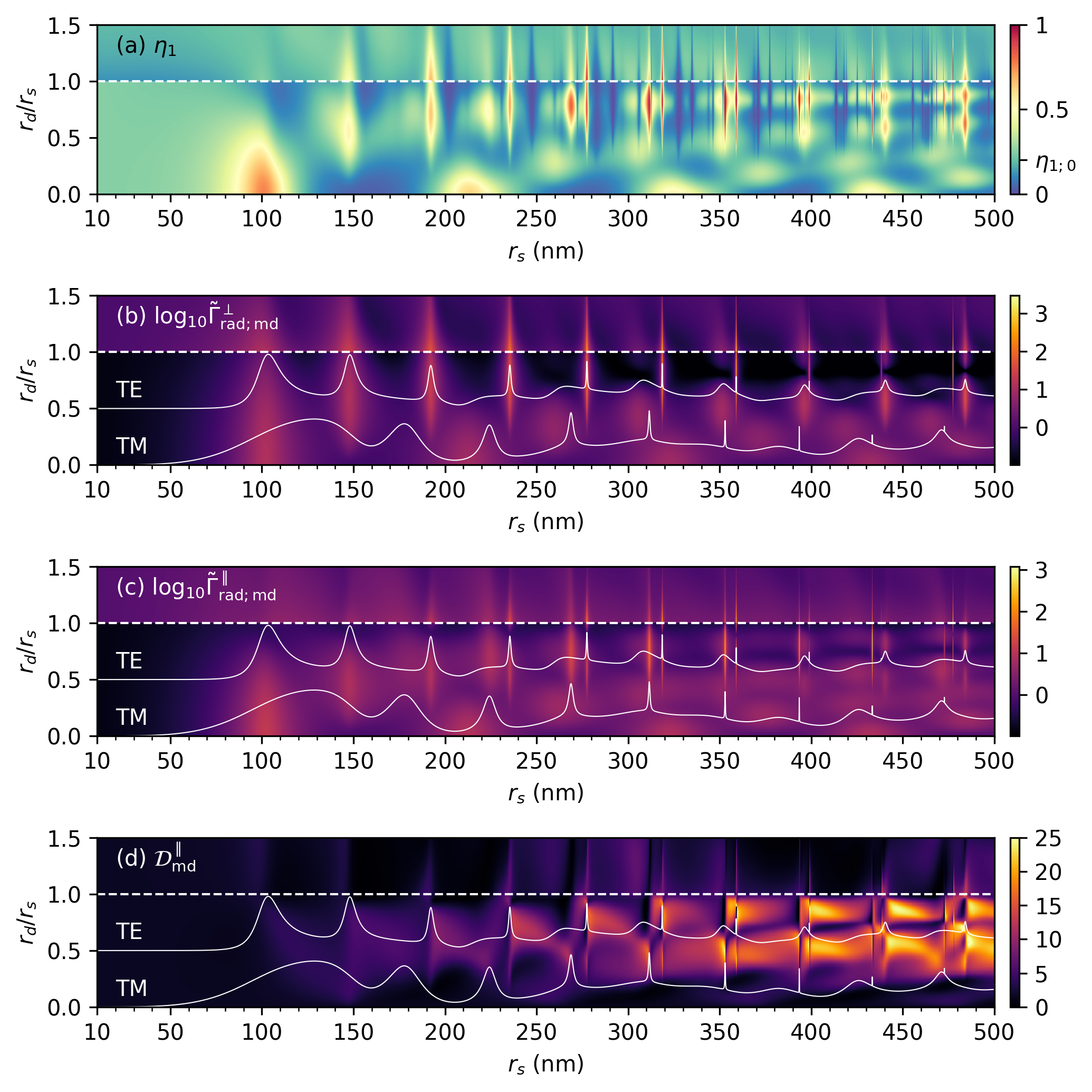
In what follows, we focus first on finding regimes with simultaneously large and , where subscript “0” denotes the respective quantity in the absence of particle. Figure 2(a) shows that the MD branching ratio approaches the limit value for a variety of sphere sizes and emitter positions. As obvious from Eq. (2), is the largest value which the branching ratio for MD transition can ever attain. Therefore, for the configurations at which approaches unity, the transitions from the parent level 5D0 level of Eu3+ are entirely dominated by the MD transition. Figure 2 shows close correlations between peaks of the branching ratio, MD radiative decay rates, and the directivity of emission of (tangentially oriented) MD with the magnetic (TE) resonances. Directivity is a relation of the power emitted into a certain direction (in our case, into the direction) to the solid angle averaged emitted power see Eq. (35) in Appendix E for details. For the parallel dipole orientation, magnetic and electric transitions have decay rate enhancement factors that are spectrally well separated. For the perpendicular dipole orientation, both electric and magnetic dipole emitters exhibit common maxima, consistent with Ref. Rolly et al. 2012. Indeed, according to Eqs. (18) and (19) (see Appendix B), one may expect radiative decay rates for the radially oriented ED and MD emitters to follow the TM and TE resonances of spheres, respectively. At the same time, the tangentially oriented ED and MD emitters exhibit enhanced radiative decay rates at both TE and TM resonances.
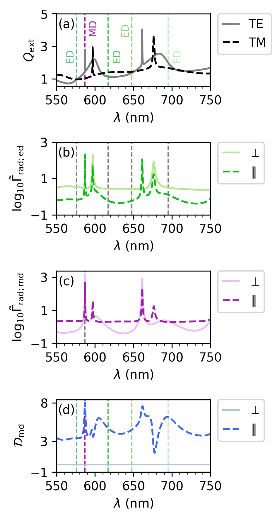
To get more insight, Fig. 3 shows wavelength-dependent extinction of TiO2 sphere with nm radius, decay rates, and directivity of Eu3+ emitter located on the surface of such a sphere. According to Fig. 2, this corresponds to and fairly large . It can be seen from Figs. 3(a-c) that the possible ED transitions of Eu3+ emitter do not correlate with any of resonances. Contrary to that, the MD transition of Eu3+ matches the magnetic (TE) resonance of a sphere. This is the physical origin behind dominant MD emission in this case. As a pleasant bonus, the MD emission for the tangentially oriented MD emitter has relatively high directivity .

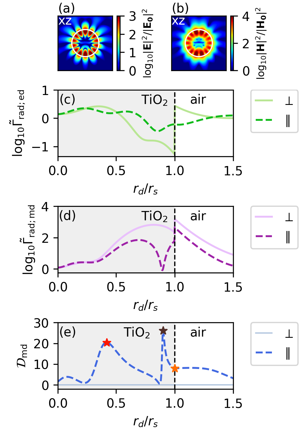
Electromagnetic fields for the TE resonances at nm corresponding to the MD transition are plotted in Figs. 4(a,b). The electric and magnetic local field distribution near TiO2 sphere enables one to identify this resonance as a multipolar resonance. In Figs. 4(c,d) it is shown how the radiative decay rate of Eu3+ depends on the position of the MD emitter inside or outside TiO2 sphere. It is worth noting that the maximum achievable radiative decay rates (for both the ED and MD transitions) occur when the emitter is located near the surface of the sphere. According to Figs. 4(c,d), the MD radiation dominates the ED radiation by several orders of magnitude for any radial position of emitter.
Interestingly, the directivity of such a system attains several maxima when the MD emitter is inside the particle, and a relatively large value when the emitter is near its surface. For a complete understanding of the formed radiation pattern in the far zone, an expansion in terms of electric (TM) and magnetic (TE) spherical harmonics was performed, indicating their amplitudes and phases. Figure 5 shows the dependencies of the directivity of a tangentially oriented MD emitter inside a TiO2 sphere in air () on the polar black angle for the cases marked in Fig. 4(e) presented in the same order. Polar angle corresponds to the direction along the negative axis. The data are presented as polar plots in the plane (left column) and plane (central column), and also the corresponding multipolar decomposition (right column). It is well known that the stored energy of different modes of a spherical resonator is concentrated in certain regions Bohren 1986. A change in the position of the magnetic dipole of a spherical resonator has a different effect on the excitation of different modes of a given resonator. Nevertheless, the energy is usually concentrated inside the dielectric. Therefore, when the dipole is placed inside, it becomes possible to adjust the amplitudes and phases of the different harmonics in such a way that all side lobes in the radiation pattern are suppressed or significantly reduced. Notably, angle-resolved directivities inside and outside the sphere are remarkably different: inside the sphere the superposition of induced multipoles leads to highly directive emission in the forward direction (Figs. 5(a,b,d,e)), while for the emitter located outside sphere, the dominant mode gives rise to a symmetrical radiation in the forward and backward directions (Figs. 5(g,h)). Note in passing that the directivity of the MD emission for the tangentially oriented emitters can achieve for the described configuration. A Fano-type behavior of the directivity in Fig. 4(e) can be explained by mixing of different multipolar modes with different amplitudes and phases induced in the sphere by the MD, as shown in Figs. 5(c,f,i). These expansions take into account both the radiation from the excited modes of the dielectric resonator and from the magnetic dipole itself.
Figure 6 demonstrates that our results can be translated to spheres with other refractive indexes and to other wavelength ranges, taking into account the respective intrinsic branching ratios and the relevant variety of ED and MD transitions of emitters under consideration. The above scalability ensures wide applicability of the presented results for magnetic light generation. For instance, our work could serve as an important tool for vibrational circular dichroism (VCD) Stephens 1985; Nafie 2004, since the very chiral signatures are attributed to the MD transitions, which enhancement is critical for sensing applications Ho et al. 2017. In this regard, recently emerged high-index iron pyrite Doiron et al. 2022 with nearly zero losses and impressively large in mid-IR range could be a very promising sphere material.

III.2 Multiple Emitters
The effect of multiple rare earth emitters on the presented above results deserves a thorough discussion. It has been known that a finite density of rare earth emitters results in the so-called concentration quenching Linares 1966; de Dood et al. 2001a; Dulkeith et al. 2005. Once an emitter is excited, it can transfer its excitation to a nearby emitter via an energy transfer mechanism. With multiple emitters present, this transfer process may end up with an eventual decay of an emitter excitation. However, if the excitation is transferred to an emitter in a proximity of an impurity (e.g., OH bonds in silica), the excitation can be swallowed up by the impurity, whereby the excitation disappears without ever contributing to either the ED or MD radiation. This is the essence of the concentration quenching. Obviously, the concentration quenching contributes to the nonradiative decay rate which origin is different from the Ohmic losses. The non-radiative decay rate is described by
| (12) |
where [Eu3+] ([]) is the emitter (quencher) concentration in at. %, and is a coupling constant). According to Eq. (2), this effect will not change the branching ratios. However, it may negatively affect the measured fluorescence signal (cf. Eq. (3)).

In order to assess the effect qualitatively, we have assumed the same quencher concentration [] as for silica in Ref. de Dood et al. 2001a. Quenchers are typically reactive OH bonds, and [] is roughly the same for all particles prepared by colloidal synthesis. The detailed procedure for estimating the coupling constant of Eu3+ emitters is presented in Appendix. The expected qualitative behavior of the concentration quenching is displayed in Fig. 7(a) with values (see Eq. (7)) depending on Eu3+ concentration, which allows us to qualitatively assess the interaction of the emitters.
Finally, it is crucial to gain insight into the possible values of ultimate fluorescence enhancement for the MD transition (), which is presented in Fig. 7(b). We take the excitation enhancement to be proportional to the surface averaged (at fixed radial distance ) intensity of the electric field, (see Ref. Rasskazov et al. 2019 for the respective closed-form expressions), and intrinsic quantum efficiency of the MD transition is according to Table 2. Being substituted in Eq. (10), these values result in the surface averaged fluorescence enhancement , which can be further increased by placing the emitter in hot spots. Since the excitation paths strongly depend on the emitter-host configuration (cf. Table 1), a sufficiently broad wavelength range is scanned to obtain a general understanding of the achievable excitation gain, which is shown in Fig. 7(c). In short, for lossless particles, exceptional electric field enhancement can be achieved at short wavelengths. The latter arises from high-order resonances (cf. Figs. 4(a,b) showing a resonance at nm), which together with an insignificant concentration quenching effect can lead to as large as , even for a significantly high concentration of Eu3+ emitters. One has also an additional freedom in selecting a suitable excitation wavelength which can be employed to optimize results even further. Clearly, the presence of losses in a particle inevitably suppresses local field enhancement and thus . Nevertheless, the proper choice of MD emitter, particle material, and excitation path can lead to significant enhancement of MD fluorescence after careful engineering of particle size and emitter position.
IV Conclusions
Magnetic light fluorescence is fundamentally different from electric light fluorescence: (i) it cannot be described by a two-level approximation involving only magnetic dipole transitions, and, because magnetic dipole transition from a particular excited level does not occur in isolation, (ii) one faces a conundrum of resolving the competition of a magnetic transition from a set of different electric dipole transitions, all from a particular excited level (see Figs. 1(c)-(d)). The latter requires to calculate for each individual transition its own radiative decay enhancement factor at the corresponding wavelength (see the Jablonski diagram in Fig. 1(c) and Table 2). Any enhancement of magnetic light fluorescence is then faced with the difficult task of identifying the regions where electric light fluorescence becomes negligible compared to magnetic light fluorescence. Despite the above difficult challenges, promising schemes to promote fluorescence of magnetic light due to the MD transitions of trivalent rare-earth ions located inside or near dielectric homogeneous spheres have been discovered.
Since the excitation enhancement amplifies all transitions by the same factor, the main objective of the sphere is to exert control over the emission processes and influence relevant branching ratios. A number of configurations involving the sphere parameters and the rare earth emitter radial position have been identified where the branching ratio of the MD transition, , approaches its limit value of unity under realistic conditions. The latter means that transitions from a certain initial excited level (e.g., 5D0 level of Eu3+) are completely dominated by the MD transition. This is truly remarkable and has never been reported before. Consequently, for properly constructed lossless dielectric spheres and for certain emitter positions, the respective values of the radiation rates and fluorescence gains for MD transitions can be larger than and , respectively. The dimensionless directivity of MD emission can reach the value of . We strongly believe that the results presented here could serve as an important tool for extending the functionality of photonic devices by promoting magnetic light.
Acknowledgements.
The work by Anton D. Utyushev, Roman Gaponenko and Alexey Shcherbakov (numerical simulations) was supported by the Russian Science Foundation, Grant No. 22-11-00153; Song Sun would acknowledge support from National Natural Science Foundation of China, Grant No. 62005256 and China Academy of Engineering Physics Innovation and Development Grant No. CX20200011.Appendix A symmetry in SI units
For an electric dipole (see Eqs. (9.4), (9.5) and (9.18) in Ref. Jackson 1999)
| (13) |
Given the Maxwell’s equations in material medium (see Eqs. (7.11) and (7.11’) in Ref. Jackson 1999) (and the vacuum case of Ref. Jackson 1999, see Eqs. (9.4) and (9.5)),
| (14) |
after the substitution, () for a magnetic dipole source will be (). Indeed, for a magnetic dipole (see Eqs. (9.33) in Ref. Jackson 1999)
| (15) |
On comparing with the first Eqs. (14), for the magnetic dipole is thus . On making use of the latter in the first of Eq. (14), one finds with the help of Maxwell’s equations in a material medium,
| (16) |
The above expressions reflect a duality symmetry of the Maxwell’s equations in the dipole case. A straightforward consequence is that
| (17) |
i.e., formally, neither the magnitude nor the orientation of the Poynting vector is changed (up to the substitution ). Therefore the decay rates (normalized to those of a free dipole) will remain the same as when calculated with and by simply interchanging the and mode labels () in the decay rates formulas of an electric dipole case.
There is no other way to interpret a MD than as a circulating current. Therefore the duality is a special duality case not covered by the conventional duality of the vacuum and the source Maxwell’s equations, the latter assuming the presence of magnetic monopoles.
Appendix B Radiative and nonradiative decay rates of electric and magnetic dipoles in a presence of a homogeneous sphere
Provided well-established results for radiative and nonradiative decay rates of electric dipole emitter located inside or outside a sphere at distance from a center of a sphere (normalized with respect to , the intrinsic radiative decay rate in the absence of a sphere) Moroz 2005,
| (18) |
one finds straightforwardly upon using symmetry from Eq. (16) the respective expressions for a magnetic dipole:
| (19) |
where , is the distance from the center of a sphere to an electric (magnetic) dipole location, is the wavevector in the medium where the emitting dipole is located ( in case if and if ), denotes the orbital angular moments (in other words, multipole number), is the Riccati-Bessel function with being the spherical Hankel function of the first kind, and prime denotes the derivative with respect to the argument in parentheses. Expressions for coefficients and , functions and , and radial integrals are provided below for convenience. For the respective detailed derivation, we refer the reader to Ref. Moroz 2005. As a reminder, subscript corresponds to electric (TM) mode, and corresponds to magnetic (TE) mode.
The coefficients and in Eqs. (18) and (19) depend on whether the decay rates were normalized with respect to the radiative decay rates in infinite homogeneous medium having the refractive index of (i) the host or (ii) the medium where the dipole is located, whether it is the host or the sphere:
| (20) |
The functions and in Eqs. (18) and (19) depend on the relative position of the emitter with respect to the sphere (inside or outside). In terms of the Riccati-Bessel functions and ,
| (21) |
where is the Riccati-Bessel function with being the spherical Bessel function of the first kind, and the numeric subscript, e.g. “21”, of the transfer-matrix (given below) corresponds to its respective element.
The respective radial integrals in Eqs. (18) and (19) are
| (22) |
Here is the wave vector in the sphere medium, and coefficients are
| (23) |
Finally, the respective backward and forward transfer matrices for the electric and magnetic modes:
| (24) |
| (25) |
| (26) |
| (27) |
where prime again denotes the derivative with respect to the argument in parentheses, and are the internal and external dimensionless size parameters, and and are sphere’s relative refractive index and permeability normalized to that of the host.
Appendix C Fluorescence quantum efficiency in the presence of nonradiative losses
Equation (7) for the fluorescence quantum efficiency of the main text,
contains absolute decay rates. Provided there is some nonradiative decay rate involved, in Eq. (7) is
| (28) |
In order to make use of Eqs. (18) and (19), Eq. (7) has to be recast in a more convenient form. Divide both the numerator and denominator of Eq. (7) with some arbitrary predetermined radiative rate ,
| (29) |
With the knowledge of that the time-averaged total radiated power of a free dipole of dipole moment is Jackson 1999
| (30) |
can be taken as the radiative decay rate of a free dipole of a unit dipole moment,
| (31) |
where we have used that . In the expressions above, , , and are the wave vector, the dielectric constant, and refractive index in the host medium. In principle, one can use for any fixed decay rate. With a single radiative channel, one can choose , whereby one recovers the usual expressions.
Appendix D Coupling constant for multiple Eu3+ emitters
Coupling constant, , entering the expression for nonradiative decay rates due to concentration quenching,
| (33) |
can be estimated from the experimental measurements for 5D0 level lifetime as a function of Eu3+ doping concentration (see Fig. 4 in Ref. Dordevic et al. 2013). Excited state lifetime is known to be inversely proportional to the total decay rate:
| (34) |
With known Lima et al. 2016 and fixed quencher concentration [], one can approximate experimental data for with a linear fit. For the data presented in Ref. Dordevic et al. 2013, we have found , which is the value used in our simulations.
Appendix E Directivity of a magnetic dipole in the presence of a sphere
By definition, the directivity is a relation of the power emitted into a certain direction to the solid angle averaged emitted power:
| (35) |
In the presence of a spherical particle, the magnetic dipole radiation pattern is modified. The respective electric and magnetic fields can be found upon using symmetry:
| (36) | |||||
| (37) |
Where the amplitudes of the outgoing radiated field are given as follows, depending on the location of the dipole with respect to a sphere:
with
| (38) | |||||
and
| (39) | |||||
The star here and above denotes the complex conjugation, which only applies to the vector spherical harmonics and not to the spherical Bessel functions Chew 1987; Chew 1988.
Normalized transverse vector multipoles are defined as
| (40) | |||||
where is an arbitrary linear combination of spherical Bessel functions ( for and for ), are vector spherical harmonics, and is a composite angular momentum index, , where the respective and label the orbital and magnetic angular numbers.
In what follows, it is expedient to introduce scalar angular functions,
| (41) |
which are defined in terms of the Wigner -functions and which can all be generated by stable recurrences. Then with the orthonormal spherical coordinate basis vectors :
| (42) | |||||
where with are the usual orthonormal scalar spherical harmonics in the Condon-Shortley convention defined in terms of the associate Legendre functions as, for instance, by Jackson Jackson 1999, and the numerical constant of Ref. Tsang et al. 1985 and numerical constant of Ref. Mishchenko 1991, are
| (43) |
, , and can be expressed as Mishchenko 1991
| (44) |
For the special case and
| (45) |
It should be remembered though that Edmonds are related to our up to prefactor of .
In the case of a magnetic dipole near a spherical particle, when both the dipole and the sphere center are located on axis , and when , the general Eq. (35) reduces to:
| (46) |
References
- Li et al. (2017) J. Li, N. Verellen, and P. Van Dorpe, Enhancing magnetic dipole emission by a nano-doughnut-shaped silicon disk, ACS Photonics 4, 1893 (2017).
- Baranov et al. (2017a) D. G. Baranov, R. S. Savelev, S. V. Li, A. E. Krasnok, and A. Alù, Modifying magnetic dipole spontaneous emission with nanophotonic structures, Laser & Photonics Reviews 11, 1600268 (2017a).
- Sanz-Paz et al. (2018) M. Sanz-Paz, C. Ernandes, J. U. Esparza, G. W. Burr, N. F. van Hulst, A. Maitre, L. Aigouy, T. Gacoin, N. Bonod, M. F. Garcia-Parajo, S. Bidault, and M. Mivelle, Enhancing magnetic light emission with all-dielectric optical nanoantennas, Nano Letters 18, 3481 (2018).
- Ernandes et al. (2018) C. Ernandes, H.-J. Lin, M. Mortier, P. Gredin, M. Mivelle, and L. Aigouy, Exploring the magnetic and electric side of light through plasmonic nanocavities, Nano Letters 18, 5098 (2018).
- Calandrini et al. (2018) E. Calandrini, A. Cerea, F. De Angelis, R. P. Zaccaria, and A. Toma, Magnetic hot-spot generation at optical frequencies: from plasmonic metamolecules to all-dielectric nanoclusters, Nanophotonics 8, 45 (2018).
- Feng et al. (2018) T. Feng, W. Zhang, Z. Liang, Y. Xu, and A. E. Miroshnichenko, Isotropic magnetic Purcell effect, ACS Photonics 5, 678 (2018).
- Bidault et al. (2019) S. Bidault, M. Mivelle, and N. Bonod, Dielectric nanoantennas to manipulate solid-state light emission, Journal of Applied Physics 126, 094104 (2019).
- Darvishzadeh-Varcheie et al. (2019) M. Darvishzadeh-Varcheie, M. Kamandi, M. Albooyeh, and F. Capolino, Optical magnetic field enhancement at nanoscale: a nanoantenna comparative study, Optics Letters 44, 4957 (2019).
- Vaskin et al. (2019) A. Vaskin, S. Mashhadi, M. Steinert, K. E. Chong, D. Keene, S. Nanz, A. Abass, E. Rusak, D.-Y. Choi, I. Fernandez-Corbaton, T. Pertsch, C. Rockstuhl, M. A. Noginov, Y. S. Kivshar, D. N. Neshev, N. Noginova, and I. Staude, Manipulation of magnetic dipole emission from Eu with Mie-resonant dielectric metasurfaces, Nano Letters 19, 1015 (2019).
- Wiecha et al. (2019) P. R. Wiecha, C. Majorel, C. Girard, A. Arbouet, B. Masenelli, O. Boisron, A. Lecestre, G. Larrieu, V. Paillard, and A. Cuche, Enhancement of electric and magnetic dipole transition of rare-earth-doped thin films tailored by high-index dielectric nanostructures, Applied Optics 58, 1682 (2019).
- Yang et al. (2019a) Y. Yang, B. F. Zhu, H. T. Dai, and X. W. Sun, Multiband enhancement of magnetic dipole emission with tapered hollow hyperbolic metamaterials, Optics Express 27, 15565 (2019a).
- Yang et al. (2019b) Y. Yang, B. Zhu, H. Dai, and X. Sun, Identical emission enhancement for arbitrary-orientation magnetic dipole emitters in silicon hollow nanocavity, Optics Express 27, 25931 (2019b).
- Wu et al. (2020) H.-W. Wu, J.-Q. Quan, Y.-Q. Yin, and Z.-Q. Sheng, Strong Purcell effect for magnetic dipole emission with spoof plasmonic spiral structure, Journal of the Optical Society of America B 37, 98 (2020).
- Aslan (2021) E. Aslan, Germanium hollow nanodisk resonator for magnetic dipole decay rate enhancement in near‐infrared, Microwave and Optical Technology Letters 63, 279 (2021).
- Aslan and Aslan (2022) E. Aslan and E. Aslan, Engineering the boosting of the magnetic Purcell factor with a composite structure based on nanodisk and ring resonators, Journal of Electromagnetic Waves and Applications 36, 1339 (2022).
- Deutschbein (1939) O. Deutschbein, Experimentelle Untersuchungen über die Vorgänge bei der Lichtemission, Annalen der Physik 428, 183 (1939).
- Walsh et al. (1998) B. M. Walsh, N. P. Barnes, and B. Di Bartolo, Branching ratios, cross sections, and radiative lifetimes of rare earth ions in solids: Application to Tm and Ho ions in LiYF, Journal of Applied Physics 83, 2772 (1998).
- Cotrufo and Fiore (2015) M. Cotrufo and A. Fiore, Spontaneous emission from dipole-forbidden transitions in semiconductor quantum dots, Physical Review B 92, 125302 (2015).
- Zurita-Sánchez and Novotny (2002) J. R. Zurita-Sánchez and L. Novotny, Multipolar interband absorption in a semiconductor quantum dot. II. Magnetic dipole enhancement, Journal of the Optical Society of America B 19, 2722 (2002).
- Bhaumik and Telk (1964) M. L. Bhaumik and C. L. Telk, Fluorescence quantum efficiency of rare-earth chelates, Journal of the Optical Society of America 54, 1211 (1964).
- Snoeks et al. (1995) E. Snoeks, A. Lagendijk, and A. Polman, Measuring and modifying the spontaneous emission rate of erbium near an interface, Physical Review Letters 74, 2459 (1995).
- Karaveli and Zia (2010) S. Karaveli and R. Zia, Strong enhancement of magnetic dipole emission in a multilevel electronic system, Optics Letters 35, 3318 (2010).
- Karaveli and Zia (2011) S. Karaveli and R. Zia, Spectral tuning by selective enhancement of electric and magnetic dipole emission, Physical Review Letters 106, 1 (2011).
- Taminiau et al. (2012) T. H. Taminiau, S. Karaveli, N. F. van Hulst, and R. Zia, Quantifying the magnetic nature of light emission, Nature Communications 3, 979 (2012).
- Aigouy et al. (2014) L. Aigouy, A. Cazé, P. Gredin, M. Mortier, and R. Carminati, Mapping and quantifying electric and magnetic dipole luminescence at the nanoscale, Physical Review Letters 113, 076101 (2014).
- Kasperczyk et al. (2015) M. Kasperczyk, S. Person, D. Ananias, L. D. Carlos, and L. Novotny, Excitation of magnetic dipole transitions at optical frequencies, Physical Review Letters 114, 163903 (2015).
- Feng et al. (2016) T. Feng, Y. Xu, Z. Liang, and W. Zhang, All-dielectric hollow nanodisk for tailoring magnetic dipole emission, Optics Letters 41, 5011 (2016).
- Choi et al. (2016) B. Choi, M. Iwanaga, Y. Sugimoto, K. Sakoda, and H. T. Miyazaki, Selective plasmonic enhancement of electric- and magnetic-dipole radiations of Er ions, Nano Letters 16, 5191 (2016).
- Rabouw et al. (2016) F. T. Rabouw, P. T. Prins, and D. J. Norris, Europium-doped NaYF nanocrystals as probes for the electric and magnetic local density of optical states throughout the visible spectral range, Nano Letters 16, 7254 (2016).
- Wiecha et al. (2018) P. R. Wiecha, A. Arbouet, A. Cuche, V. Paillard, and C. Girard, Decay rate of magnetic dipoles near nonmagnetic nanostructures, Physical Review B 97, 085411 (2018).
- Mashhadi et al. (2019) S. Mashhadi, M. Durach, D. Keene, and N. Noginova, Control of magnetic dipole emission with surface plasmon polaritons, OSA Continuum 2, 1342 (2019).
- Zhong and Goldner (2019) T. Zhong and P. Goldner, Emerging rare-earth doped material platforms for quantum nanophotonics, Nanophotonics 8, 2003 (2019).
- Kalinic et al. (2020) B. Kalinic, T. Cesca, S. Mignuzzi, A. Jacassi, I. G. Balasa, S. A. Maier, R. Sapienza, and G. Mattei, All-dielectric silicon nanoslots for Er photoluminescence enhancement, Physical Review Applied 14, 014086 (2020).
- Alaee et al. (2020) R. Alaee, B. Gurlek, M. Albooyeh, D. Martín-Cano, and V. Sandoghdar, Quantum metamaterials with magnetic response at optical frequencies, Physical Review Letters 125, 063601 (2020).
- Sun et al. (2022) S. Sun, D. Li, D. Wang, Z. Feng, W. Tan, and L. Wu, Empowering magnetic strong coupling and its application for nonlinear refractive index sensing, Nano Research 15, 7604 (2022).
- Bharadwaj et al. (2009) P. Bharadwaj, B. Deutsch, and L. Novotny, Optical antennas, Advances in Optics and Photonics 1, 438 (2009).
- Krasnok et al. (2013) A. E. Krasnok, I. S. Maksymov, A. I. Denisyuk, P. A. Belov, A. E. Miroshnichenko, C. R. Simovski, and Y. S. Kivshar, Optical nanoantennas, Physics-Uspekhi 56, 539 (2013).
- Klimov and Letokhov (2005) V. V. Klimov and V. S. Letokhov, Electric and magnetic dipole transitions of an atom in the presence of spherical dielectric interface, Laser Physics 15, 61 (2005).
- Schmidt et al. (2012) M. K. Schmidt, R. Esteban, J. J. Sáenz, I. Suárez-Lacalle, S. Mackowski, and J. Aizpurua, Dielectric antennas - a suitable platform for controlling magnetic dipolar emission, Optics Express 20, 13636 (2012).
- Rolly et al. (2012) B. Rolly, B. Bebey, S. Bidault, B. Stout, and N. Bonod, Promoting magnetic dipolar transition in trivalent lanthanide ions with lossless Mie resonances, Physical Review B 85, 245432 (2012).
- Zambrana-Puyalto and Bonod (2015) X. Zambrana-Puyalto and N. Bonod, Purcell factor of spherical Mie resonators, Physical Review B 91, 195422 (2015).
- Chigrin et al. (2016) D. N. Chigrin, D. Kumar, D. Cuma, and G. von Plessen, Emission quenching of magnetic dipole transitions near a metal nanoparticle, ACS Photonics 3, 27 (2016).
- Zhao et al. (2019) Q. Zhao, Z.-J. Yang, and J. He, Coherent couplings between magnetic dipole transitions of quantum emitters and dielectric nanostructures, Photonics Research 7, 1142 (2019).
- Habil et al. (2021) M. K. Habil, C. J. Zapata–Rodríguez, M. Cuevas, and S. R. Entezar, Multipolar-sensitive engineering of magnetic dipole spontaneous emission with a dielectric nanoresonator antenna, Scientific Reports 11, 12813 (2021).
- Hu et al. (2022) M.-L. Hu, X.-J. Du, L. Ma, J. He, and Z.-J. Yang, Strong superradiance of coherently coupled magnetic dipole emitters mediated by whispering gallery modes of a subwavelength all-dielectric cavity, Physical Review B 106, 205420 (2022).
- Cheng et al. (2021) X. Cheng, X. Zhuo, R. Jiang, Z. Wang, J. Wang, and H. Lin, Electromagnetic resonance‐modulated magnetic emission in europium‐doped sub‐micrometer zirconia spheres, Advanced Optical Materials 9, 2002212 (2021).
- Sugimoto and Fujii (2021) H. Sugimoto and M. Fujii, Magnetic Purcell enhancement by magnetic quadrupole resonance of dielectric nanosphere antenna, ACS Photonics 8, 1794 (2021).
- de Dood et al. (2001a) M. J. A. de Dood, L. H. Slooff, A. Polman, A. Moroz, and A. van Blaaderen, Modified spontaneous emission in erbium-doped SiO spherical colloids, Applied Physics Letters 79, 3585 (2001a).
- de Dood et al. (2001b) M. J. A. de Dood, L. H. Slooff, A. Polman, A. Moroz, and A. van Blaaderen, Local optical density of states in SiO spherical microcavities: Theory and experiment, Physical Review A 64, 033807 (2001b).
- Yao and Zheng (2021) K. Yao and Y. Zheng, Directional light emission by electric and magnetic dipoles near a nanosphere: an analytical approach based on the generalized Mie theory, Optics Letters 46, 302 (2021).
- Neuman et al. (2020) T. Neuman, D. S. Wang, and P. Narang, Nanomagnonic cavities for strong spin-magnon coupling and magnon-mediated spin-spin interactions, Physical Review Letters 125, 247702 (2020).
- Deng et al. (2022) Q. Deng, J. Chen, L. Long, B. Chen, H. Yu, and Z. Li, Silicon cuboid nanoantenna with simultaneous large Purcell factor for electric dipole, magnetic dipole and electric quadrupole emission, Opto-Electronic Advances 5, 210024 (2022).
- Mi et al. (2019) H. Mi, L. Wang, Y. Zhang, G. Zhao, and R. Jiang, Control of the emission from electric and magnetic dipoles by gold nanocup antennas, Optics Express 27, 14221 (2019).
- Pan et al. (2022) G.-M. Pan, L.-F. Yang, F.-Z. Shu, Y.-L. Meng, Z. Hong, and Z.-J. Yang, Tailoring magnetic dipole emission by coupling to magnetic plasmonic anapole states, Photonics Research 10, 2032 (2022).
- Brûlé et al. (2022) Y. Brûlé, P. Wiecha, A. Cuche, V. Paillard, and G. Colas des Francs, Magnetic and electric Purcell factor control through geometry optimization of high index dielectric nanostructures, Optics Express 30, 20360 (2022).
- Reynier et al. (2023) B. Reynier, E. Charron, O. Markovic, X. Yang, B. Gallas, A. Ferrier, S. Bidault, and M. Mivelle, Full control of electric and magnetic light–matter interactions through a nanomirror on a near-field tip, Optica 10, 841 (2023).
- García‐Puente and Kashyap (2023) Y. García‐Puente and R. Kashyap, Magnetic Purcell enhancement in a nanoantenna‐spherical Bragg resonator coupled system, Annalen der Physik , 2300147 (2023).
- Yi et al. (2016) X. Yi, J. Sun, X.-F. Jiang, Y. Li, Q.-H. Xu, Q. Zhang, and S. Ye, Variations in the D→F transitions of Eu and white light emissions in Ag–Eu exchanged zeolite-Y, RSC Advances 6, 95925 (2016).
- Luewarasirikul and Kaewkhao (2021) N. Luewarasirikul and J. Kaewkhao, Spectroscopic properties and Judd-Ofelt analysis of Eu doped Ba-Na-B glasses for photonic applications, Journal of Physics: Conference Series 1819, 012072 (2021).
- Kolesnikov et al. (2016) I. E. Kolesnikov, A. V. Povolotskiy, D. V. Mamonova, E. Lähderanta, A. A. Manshina, and M. D. Mikhailov, Photoluminescence properties of Eu ions in yttrium oxide nanoparticles: defect vs. normal sites, RSC Advances 6, 76533 (2016).
- Iwanaga (2019) H. Iwanaga, Photoluminescence properties of Eu(III) complexes with thienyl-substituted diphosphine dioxide ligands, Bulletin of the Chemical Society of Japan 92, 1385 (2019).
- Sai et al. (2022) D. S. Sai, K. Swapna, K. Deepthi, J. V. S. Kumar, S. Mahamuda, M. Venkateswarlu, P. Sruthi, D. Amer, and A. S. Rao, Spectroscopic studies of Eu ion-doped antimony-lead-oxyfluoroborate glasses for visible red photonic device applications, Journal of Electronic Materials 51, 3980 (2022).
- Judd (1962) B. R. Judd, Optical absorption intensities of rare-earth ions, Physical Review 127, 750 (1962).
- Ofelt (1962) G. S. Ofelt, Intensities of crystal spectra of rare‐earth ions, Journal of Chemical Physics 37, 511 (1962).
- Linares (1966) R. C. Linares, Fluorescent properties of trivalent rare earths in fluorite structure oxides, Journal of the Optical Society of America 56, 1700 (1966).
- Rikken and Kessener (1995) G. L. J. A. Rikken and Y. A. R. R. Kessener, Local field effects and electric and magnetic dipole transitions in dielectrics, Physical Review Letters 74, 880 (1995).
- Nagaishi et al. (2003) R. Nagaishi, T. Kimura, and S. P. Sinha, Luminescence properties of lanthanide(III) ions in concentrated carbonate solution, Molecular Physics 101, 1007 (2003).
- Moroz (2005) A. Moroz, A recursive transfer-matrix solution for a dipole radiating inside and outside a stratified sphere, Ann. Phys. (NY) 315, 352 (2005).
- Bharadwaj and Novotny (2007) P. Bharadwaj and L. Novotny, Spectral dependence of single molecule fluorescence enhancement, Optics Express 15, 14266 (2007).
- Sugimoto et al. (2021) H. Sugimoto, H. Hasebe, T. Furuyama, and M. Fujii, Direct excitation of triplet state of molecule by enhanced magnetic field of dielectric metasurfaces, Small 17, 2104458 (2021).
- Freed and Weissman (1941) S. Freed and S. I. Weissman, Multiple nature of elementary sources of radiation—wide-angle interference, Physical Review 60, 440 (1941).
- Conde-Gallardo et al. (2001) A. Conde-Gallardo, M. Garcıa-Rocha, I. Hernandez-Calderón, and R. Palomino-Merino, Photoluminescence properties of the Eu activator ion in the TiO host matrix, Applied Physics Letters 78, 3436 (2001).
- Aihua Peng et al. (2005) Aihua Peng, Erqing Xie, Changwen Jia, Ran Jiang, and Hongfeng Lin, Photoluminescence properties of TiO:Eu thin films deposited on different substrates, Materials Letters 59, 3866 (2005).
- Antic et al. (2012) Z. Antic, R. M. Krsmanovic, M. G. Nikolic, M. Marinovic-Cincovic, M. Mitric, S. Polizzi, and M. D. Dramicanin, Multisite luminescence of rare earth doped TiO anatase nanoparticles, Materials Chemistry and Physics 135, 1064 (2012).
- Reszczyńska et al. (2016) J. Reszczyńska, T. Grzyb, Z. Wei, M. Klein, E. Kowalska, B. Ohtani, and A. Zaleska-Medynska, Photocatalytic activity and luminescence properties of RE–TiO nanocrystals prepared by sol–gel and hydrothermal methods, Applied Catalysis B: Environmental 181, 825 (2016).
- Gao et al. (2022) F. Gao, X. Zhao, and J. Liu, A facile method for the fabrication of luminescent Eu-doped SiO nanowires, Gels 8, 286 (2022).
- Liu et al. (2011) Y. Liu, W. Luo, H. Zhu, and X. Chen, Optical spectroscopy of lanthanides doped in wide band-gap semiconductor nanocrystals, Journal of Luminescence 131, 415 (2011).
- Chen et al. (2021) D. Chen, S. Miao, Y. Liang, W. Wang, S. Yan, J. Bi, and K. Sun, Controlled synthesis and photoluminescence properties of BiSiO:Eu core-shell nanospheres with an intense D→F transition, Optical Materials Express 11, 355 (2021).
- Wei et al. (2012) R. Wei, J. Li, J. Gao, and H. Guo, Enhancement of Eu luminescence by Ag species (Ag Ns, ML-Ag,Ag) in oxyfluoride glasses, Journal of the American Ceramic Society 95, 3380 (2012).
- Sun et al. (2020) S. Sun, I. L. Rasskazov, P. S. Carney, T. Zhang, and A. Moroz, Critical role of shell in enhanced fluorescence of metal-dielectric core-shell nanoparticles, Journal of Physical Chemistry C 124, 13365 (2020).
- Rasskazov et al. (2021) I. L. Rasskazov, A. Moroz, and P. S. Carney, Extraordinary fluorescence enhancement in metal-dielectric core-shell nanoparticles, Journal of Physical Chemistry Letters 12, 6425 (2021).
- Lima et al. (2016) N. B. D. Lima, J. D. L. Dutra, S. M. C. Gonçalves, R. O. Freire, and A. M. Simas, Chemical partition of the radiative decay rate of luminescence of europium complexes, Scientific Reports 6, 21204 (2016).
- Jackson (1999) J. D. Jackson, Classical electrodynamics (John Wiley & Sons, Inc., 1999).
- Rasskazov et al. (2020) I. L. Rasskazov, P. S. Carney, and A. Moroz, STRATIFY: a comprehensive and versatile MATLAB code for a multilayered sphere, OSA Continuum 3, 2290 (2020).
- Baranov et al. (2017b) D. G. Baranov, D. A. Zuev, S. I. Lepeshov, O. V. Kotov, A. E. Krasnok, A. B. Evlyukhin, and B. N. Chichkov, All-dielectric nanophotonics: the quest for better materials and fabrication techniques, Optica 4, 814 (2017b).
- van Blaaderen and Vrij (1992) A. van Blaaderen and A. Vrij, Synthesis and characterization of colloidal dispersions of fluorescent, monodisperse silica spheres, Langmuir 8, 2921 (1992).
- Gritsch et al. (2022) A. Gritsch, L. Weiss, J. Früh, S. Rinner, and A. Reiserer, Narrow optical transitions in erbium-implanted silicon waveguides, Physical Review X 12, 041009 (2022).
- Dulkeith et al. (2005) E. Dulkeith, M. Ringler, T. A. Klar, J. Feldmann, A. Muñoz Javier, and W. J. Parak, Gold nanoparticles quench fluorescence by phase induced radiative rate suppression, Nano Letters 5, 585 (2005).
- Acuna et al. (2012) G. P. Acuna, M. Bucher, I. H. Stein, C. Steinhauer, A. Kuzyk, P. Holzmeister, R. Schreiber, A. Moroz, F. D. Stefani, T. Liedl, F. C. Simmel, and P. Tinnefeld, Distance dependence of single-fluorophore quenching by gold nanoparticles studied on DNA origami, ACS Nano 6, 3189 (2012).
- Bohren (1986) C. F. Bohren, Applicability of effective-medium theories to problems of scattering and absorption by nonhomogeneous atmospheric particles, Journal of the Atmospheric Sciences 43, 468 (1986).
- Stephens (1985) P. J. Stephens, Theory of vibrational circular dichroism, Journal of Physical Chemistry 89, 748 (1985).
- Nafie (2004) L. A. Nafie, Theory of vibrational circular dichroism and infrared absorption: Extension to molecules with low-lying excited electronic states, Journal of Physical Chemistry A 108, 7222 (2004).
- Ho et al. (2017) C.-S. Ho, A. Garcia-Etxarri, Y. Zhao, and J. Dionne, Enhancing enantioselective absorption using dielectric nanospheres, ACS Photonics 4, 197 (2017).
- Doiron et al. (2022) C. F. Doiron, J. B. Khurgin, and G. V. Naik, Super‐Mossian dielectrics for nanophotonics, Advanced Optical Materials 10, 2201084 (2022).
- Dolgaleva and Boyd (2012) K. Dolgaleva and R. W. Boyd, Local-field effects in nanostructured photonic materials, Advances in Optics and Photonics 4, 1 (2012).
- Rasskazov et al. (2019) I. L. Rasskazov, A. Moroz, and P. S. Carney, Electromagnetic energy in multilayered spherical particles, Journal of the Optical Society of America A 36, 1591 (2019).
- Dordevic et al. (2013) V. Dordevic, Z. Antic, M. Nikolic, and M. Dramicanin, The concentration quenching of photoluminescence in eu3+-doped la2o3, Journal of Research in Physics 37, 47 (2013).
- Chew (1987) H. Chew, Transition rates of atoms near spherical surfaces, Journal of Chemical Physics 87, 1355 (1987).
- Chew (1988) H. Chew, Radiation and lifetimes of atoms inside dielectric particles, Physical Review A 38, 3410 (1988).
- Tsang et al. (1985) L. Tsang, J. A. Kong, and R. T. Shin, Theory of Microwave Remote Sensing (Wiley, 1985).
- Mishchenko (1991) M. I. Mishchenko, Light scattering by randomly oriented axially symmetric particles, Journal of the Optical Society of America A 8, 871 (1991).