Building the Standard Model
Historical and Qualitative Aspects

Feynman entered QED with his famous intiution and he solved the equations without the complicated machinery with field operators. As I understood it, he studied a priori differential equations for scattering of an electron in an electromagnetic field. Then these equations were adapted to more complicated processes. This method, often named the “Feynman approach” is nicely described in the old book “Relativistic quantum mechanics” written by Bjorken and Drell Bjorken:1965sts. I learned, and later lectured, some times this version which is theoretically simplified compared to standard QED with all the operator formalism. However, there is an important warning: Using this simplified version, the Pauli principle had to be put in by hand!,- in contrast to true QED field theory, where all the correct signs are automatially obtained by the anticommuting fields. The well known equations to be solved are

$$\left(\gamma_{\mu}\,(i\partial^{\mu}\,-\,eA^{\mu}(x))-\,m\right)\,\Psi(x)\,=\,0\quad;\;\;\partial_{\nu}\partial^{\nu}\,A^{\mu}(x)\,=\,ej_{D}^{\mu}(x)\;,$$

(1)

where $e$ is the elementary electron charge. Further, $A^{\mu}(x)$ is the electromagnetic field and $\Psi(x)$ is the electron field which would in the non-relativistic case correspond to the electron wave function. Here Lorentz gauge for the electromagnetic field is assumed:

$$\partial_{\nu}A^{\nu}(x)\,=0\;.$$

(2)

Now, for the electromagnetic current in a scattering process one writes the Dirac current as the transition current

$$j_{D}^{\mu}(x)\,=\,\overline{\psi(x)}_{b}\gamma^{\mu}\psi(x)_{a}\;,$$

(3)

where $\psi(x)_{a}$ represents an ingoing (asymtotically) free electron in some chosen process and $\overline{\psi(x)}_{b}$ represents an outgoing (asymtotically) free electron in the same process.

The differential equation for $\Psi(x)$ in (1) can be rewritten

$$\left(\gamma_{\mu}\,(i\partial^{\mu}\,-\,eA^{\mu}(x))-\,m\right)\,\Psi(x)\,=\;eA^{\mu}(x)\gamma_{\mu}\Psi(x)\;,$$

(4)

The equation in (4) for $\Psi$ and the equation for $A^{\mu}$ in (1) may be solved by free Green-functions $S_{F}(x-y)$ for the free Dirac Field $\Psi(x)$ and $D_{F}(x-y)$ for the free vector field $A^{\mu}(x)$ respectively :

$$\left(i\gamma_{\mu}\partial^{\mu}\,-\,m\right)S_{F}(x-y)={\bf 1}^{(D)}\delta^{(4)}(x-y)\quad,\;\;\mbox{and}\;\,\partial_{\nu}\partial^{\nu}D_{F}(x-y)_{\alpha\beta}=\delta_{\alpha\beta}\delta^{(4)}(x-y),$$

(5)

where ${\bf 1}^{(D)}$ is the unit matrix in the space of Dirac matrices, and $\mu,\nu,\alpha,\beta$ are Lorentz indices. These Greens functions will (for proper boundary conditions ) also be the propagators for the particles. They are given by

$$S_{F}(x-y)=\int\frac{d^{4}p}{(2\pi^{4}}\frac{(\gamma\cdot p\,+\,m)}{(p^{2}-m^{2}+i\epsilon)}\;\,,\mbox{and}\qquad D_{F}(x-y)_{\alpha\beta}=\int\frac{d^{4}k}{(2\pi^{4})}\frac{(-g_{\alpha\beta})}{(k^{2}+i\epsilon)}\;\,.$$

(6)

Here the small $\epsilon$ takes care of the asymtotic properties of the propagator (for $\epsilon\rightarrow 0$) For the electron(fermion)propagator one also obtains :

$$S_{F}(x-y)=\theta(x_{0}-y_{0})\sum_{\sigma}\int\frac{d^{3}p}{(2\pi)^{3}}\psi^{(+)}_{p\sigma}(x)\overline{\psi^{(+)}_{p\sigma}(y)}\,-\,\theta(y_{0}-x_{0})\sum_{\sigma}\int\frac{d^{3}p}{(2\pi)^{3}}\psi^{(-)}_{p\sigma}(x)\overline{\psi^{(-)}_{p\sigma}(y)}\;,$$

(7)

where $\psi^{(\pm)}_{p\sigma}(x)$ are plane wave solutions of the Dirac equation with definite momentum ($p$)and spin quantum number $\sigma$, and energy sign $\epsilon=\pm$. $\psi^{(+)}$ and $\psi^{(-)}$ represent the particle and anti-particle solutions respectively. As usual $\overline{\psi}=(psi)^{d}agger\,\gamma_{0}$. A similar expression for the photon propagator is cumbersome because of the gauge freedom for the photon field. The photon propagator is presented in various ways, for instance via path integrals.

For the interacting electron field one obtains the solution:

$$\Psi(x)_{i}\,=\,\psi(x)_{i}\,+\,\int d^{4}y\,S_{F}(x-y)\,e\gamma^{\mu}A_{\mu}(y)\,\Psi(y)_{i}\;\,,$$

(8)

where $\Psi(x)_{i}$ is the solution when $\psi(x)_{i}$ is the ingoing plane wave. As it stands, this solution looks useless because the unknown solution $\Psi(x)_{i}$ is also under the integral at the right hand side. In order to obtain useful result one solves the equation iteratively, or in other words, perturbatively:

$$\Psi(x)_{i}\,=\,\sum_{n}\Psi(x)^{(n)}_{i}\;,$$

(9)

where $\Psi(x)^{(0)}_{i}=\psi(x)_{i}$ and the $n$’th term is given by

$$\Psi(x)^{(n)}_{i}\,=\,\,\int d^{4}y\,S_{F}(x-y)\,e\gamma^{\mu}A_{\mu}(y)\,\Psi(y)^{(n-1)}_{i}\;\,.$$

(10)

This gives the first non-trivial approximation

$$\Psi(x)^{(1)}_{i}\,=\,\,\int d^{4}y\,S_{F}(x-y)\,e\gamma^{\mu}A_{\mu}(y)\,\psi(y)_{i}\;\,.$$

(11)

Further, the second term is

$$\Psi(x)^{(2)}_{i}\,=\,\,\int\int d^{4}y\,d^{4}zS_{F}(x-y)\,e\gamma^{\mu}A_{\mu}(y)\,S_{F}(y-z)e\gamma^{\nu}A_{\nu}(z)\psi(z)_{i}\;\,,$$

(12)

and so on.

The solution for the electromagnetic field is:

$$A^{\mu}(x)\,=\,A^{\mu}_{0}(x)\,+\,\int d^{4}y\,D_{F}(x-y)^{\mu\nu}\,ej_{\nu D}(y)\;\,,$$

(13)

where $A^{\mu}_{0}(x)$ is the initial (some times the final) free solution electromagnetic field, depending on the process which is considered, and $j_{D}^{\mu}(y)$ given in (3). When there are no photons in the initial or final state, then $A^{\mu}_{0}(x)$ is zero.

The scattering matrix is -for a given initial state $\psi_{i}$ - the probability amplitude to measure a chosen final state $\psi_{f}$ to occur. Thus the scattering matrix is given by a scalar product of the interacting $\Psi_{i}$ and the chosen final plane wave $\psi(x)_{f}$ :

$$S_{fi}\,=\,\left(\psi(x)_{f},\Psi(x)_{i}\right)_{x_{0}\rightarrow\epsilon_{f}\infty}=\,\delta_{fi}\,+\,\int d^{4}y\,e\,\overline{\psi(y)_{f}}\,\gamma^{\mu}A_{\mu}(y)\,\Psi(y)_{i}\;\,.$$

(14)

Here $x_{0}\rightarrow\,+\infty$ when $\psi_{f}$ is a particle (positive frequency $\epsilon_{f}$ = +1) and $x_{0}\rightarrow\,-\infty$ when $\psi_{f}$ is an antiparticle (negative frequency $\epsilon_{f}$ = -1). This means that mathematically, in outgoing(ingoing) particle with negative energy is intepreted as an ingoing(outgoing) antiparticle.

The scattering matrix can be written as a perturbation series, when $\Psi(y)_{i}$ is given by equation (9):

$$S_{fi}\,=\,\sum_{n}\;S_{fi}^{(n)}\quad\mbox{where}\;\;S_{fi}^{(0)}=\delta_{fi}\;\,,$$

(15)

and further, the first nontrivial term is

$$S_{fi}^{(1)}\,=\,\epsilon_{f}\,e\,\int d^{4}y\,\overline{\psi(y)_{f}}\,\gamma^{\mu}A_{\mu}(y)\,\psi(y)_{i}\;\,.$$

(16)

Here we obtain simple scattering of an electron in a Coulomb field $A^{\mu}_{0}=A^{\mu}_{Coul}$ and put $j_{D}^{\mu}=0$ in (13). Or, alternatively, we may put $A^{\mu}_{0}=0$ and use a suitable Dirac current $j^{\mu}_{D}$ for an in- and out-going electron(positron); see equation (3). Then we describe scattering of an electron (positron) in the field of another electron(positron), that is, we may describe electron-electron (Møller) scattering or electron-positron (Bhabha) scattering;- provided we symmetrise the following amplitude according to the Pauli principle. Mathematically, for a relevant contribution

$$S_{fi}^{(1,j_{D})}\,=\,\epsilon_{f}\,e\,\int d^{4}y\,\overline{\psi(y)_{f}}\,\gamma^{\mu}\psi(y)_{i}\,\int d^{4}xD_{F}(x-y)_{\mu\nu}\,[e\overline{\psi(x)_{b}}\gamma^{\nu}\psi(x)_{a}]\;\,.$$

(17)

In standard QED this would correspond to a second a second order contribution from the scattering operator contribution.

The next non-trivial term is

$$S_{fi}^{(2)}\,=\,\epsilon_{f}e^{2}\,\int\int d^{4}y\,d^{4}z\,\overline{\psi(y)_{f}}\,\gamma^{\mu}A_{\mu}(y)\,\,S_{F}(y-z)e\gamma^{\nu}A_{\nu}(z)\psi(z)_{i}\;\,,$$

(18)

which may describe Compton scattering, or $e^{+}\,e^{-}\rightarrow\gamma\gamma$ annihilation , or pair creationn $\gamma\gamma\rightarrow e^{+}e^{-}$.

The method described above works, and gives the same result as the QED with the fields as operators, (again!:) provided that the minus sign is used if the final electron is an antiparticle. Antiparticles (positrons) are represented by negative enrgy electrons going backwards in time. There is also the obscure intepretation of the negative energy solutions filling up the “Dirac sea”. In QED with anticommuting fermion field operators the correct relative signs come out automatic, and the obscure Dirac sea disappears. Note that (18) has the same form as the second order expression in QED where the $\psi$’s are field operators, except for the factor $1/(2!)$. However such statistical factors typically disappears (replaced by the number one) when Wicks theorem are applied for the field operators. Some lecturers do not mention this “relativistic quantum mechanics” (“Feynman approach”) because of its shortcomings. Others thinks it is OK to see how close one might come with some intiution.

The QED Lagrangian may be written

$${\cal L}_{QED}\,=\,$$

(19)

$$\overline{\psi(x)}\left(i\gamma_{\mu}\,\partial^{\mu}\,-\,m\right)\,\psi(x)\hskip 28.45274pt\rightarrow(\mbox{electron propagator})$$

(20)

$$-\frac{1}{4}F_{\mu\nu}(x)\,F^{\mu\nu}(x)\hskip 71.13188pt\rightarrow(\mbox{photon propagator})$$

(21)

$$-ieA_{\mu}(x)\,\left(\overline{\psi(x)}\gamma_{\mu}\psi(x)\right)\hskip 36.98866pt\rightarrow(\mbox{interaction})\;,$$

(22)

where $F_{\mu\nu}$ is, as described in some textbooks, given by the commutator of two covariant derivatives $iD_{\lambda}=\partial_{\lambda}\,\,-\,eA_{\lambda}$:

$$ie\,F_{\mu\nu}(x)\;=\;[iD_{\mu}\,,\,iD_{\nu}]\,=\,ie(\partial_{\mu}A_{\nu}\,-\,\partial_{\nu}A_{\mu})$$

(23)

Using standard canonical quantisation, from this Lagrangian one may calculate all processe in QED. But one should note some important points.:

In relativistic physics, particles may appear and disappear as quantum fluctuations (loop effects) as long as the two quantities energy and electric charge are conserved!

Further, a free electron should be stable. This corsponds to the $\delta_{fi}\,=\,1$ with $f=i$. This means that the integral in (14) should not contribute to the S-matrix for a free electron. However, a concrete calculation shows that this requirement is not fulfilled. This means that for the electron part one obtains a factor different from one in front of the first term in (20). To solve this problem, one has to realize that the fields in the Lagrangian above are bare fields. The physical renormalized fields, dressed with loop effects are $\Psi_{R}=\sqrt{Z_{F}}\Psi_{0}$, where $\Psi_{0}$ is the bare field in the Lagrangian above, and $Z_{F}$ represent the loop effects. Also the mass term in (20) has to be renormalised ($m_{0}\rightarrow m_{R}$). And also the photon term (21) and the interaction term (22) has also to be renormalized. This will be discussed in the following subsections.

In Fig. 1 the left diagram (just the electron line) corresponds to the bare electron propagator. The lowest order correction to the electron propagator (20) contribution to the electron paropagator, is given in the middle. As already mentioned, the electron is stable, and the theory(QED) should be constistent with this fact. Therefore the $S$-matrix element corresponding to the to the diagram in Fig. 2 (lowest order self energy) should be zero for an electron on the physical mass-shell $p^{2}=m^{2}$.(Also for $\gamma\cdot p\rightarrow m)$. A concrete calculation shows that this is not the case. In order to solve this problem , one has to redefine the mass and write

$$m_{R}\;\,=\;\,m_{0}\,-\,\delta m\;\,,$$

(24)

where $m_{0}$ is the bare mass contained in (20) and $\delta m$ is the result from the diagram in the middle of Fig. 2. Now the right diagram in Fig. 2 (the counterterm) with the cross to the right substracts the value of diagram 1b to get zero on-shell $p^{2}=m_{R}^{2}$. An a priori disturbing discovery was also that $\delta m$ was infinite, and could be parametrised through a cut-off $\Lambda$ :

$$\delta m\,=m_{0}\,\frac{\alpha}{4\pi}ln(\frac{\Lambda^{2}}{m_{0}^{2}})\,.$$

(25)

Moreover, it can be shown that in order to get the propagator pole at $m_{R}$, the electron part has to be multiplied by a additional factor $Z_{F}=1+k\frac{\alpha}{4\pi}ln(\frac{\Lambda^{2}}{m_{0}^{2}})$ where $k$ is some number of order one given by the loop integration. Then also the pole of the electron propagator will be shifted from $p^{2}=m_{0}^{2}$ in (6 ) to the correct place, $p^{2}=m_{R}^{2}$. Still the remaining part of diagram in Fig. 2 for off-shell electrons are nonzero! It turns out that for a bound electron (which is off-shell) in a Hydrogen atom this non-zero off-shell part will give the main contribution to Lamb-shift. Namely: The degenerations of $2S_{1/2}$ and $2P_{1/2}$ in Hydrogen are now removed (lifted) by the (renormalized) self-energy contribution for bound (off-shell) electrons. This gives the famous Lamb-shift in Hydrogen giving the $\lambda\simeq$ 21 cm line.

Within non-relativistic quantum mechanics, and also for the relativistic equation of Dirac, the gyromagnetic factor of the electron is $g_{e}=2$. Entering QED, there are corrections to this result. Now the diagram in the middle of Fig. 3 will give a contribution(correction) to the gyromagnetic factor. Also here there is a diagram (a counterterm) to the right of Fig.3 to subtract unphysical terms via renormalisation.

Now the remaining vertex correction ( the middle of Fig. 3 ) gives a small correction to $g_{e}$ such that with the lowest order correction, the result is

$$g_{e}\,=\,2+\frac{\alpha_{em}}{\pi}$$

(26)

In Fig 4 the left diagram, just the wavy line, represents the bare photon propagator in (21). The diagram in the middle of Fig 4 gives a corrections to the photon propagator, usually called the vacuum polarisation diagram. Adding the conterterm in 4c will stabilise the photon.

The diagram in the middle of Fig. 4 means that electron-positron pairs appear and disappears (as quantum fluctuations). This can be seen as screening of electric charge, which gives an energy dependent fine structure “constant” $\alpha_{em}$. Previously this diagram(s) were interpreted as a correction to the Coulomb potential. Now, in modern field theory, one usually intepretes this as an energy dependent effective fine structure. This means that $\alpha_{em}\,=\,\frac{1}{137}$ for low energy photons. The momentum-energy dependent fine structure factor is $\alpha_{em}(q^{2})\,>\,\frac{1}{137}$ for larger energies. Also this means thet the electric charge in eq. (22) is the bare charge $e_{0}$. Adding later also other charged particles in the loop, i.e more charged leptons, quarks and also the charged W-bosons, make $\alpha_{em}\,\simeq\,\frac{1}{128}$ at the energy $M_{Z}c^{2}$.

One tried to construct a theory for interactions between pions and nucleons as a field theory where photons were replaced by pions and electrons by nucleons in an isospin symmetric way.

The isospin symmetric interaction Lagrangian for strong interactions: was written down as

$\displaystyle{\cal L}_{\pi N}\;=\;G_{\pi N}\,\bar{N}\,(\tau_{i}\,\Phi_{i})\,\gamma_{5}\,N\;\;,\;N\;=\;\left(\begin{array}[]{c}p\\ n\end{array}\right)\;\,,$

where $N$ is the nucleon doublet, $\Phi$ the pion triplet and $\tau$ the Pauli matrices which here represents isospin. Here

$\displaystyle\pi^{\pm}\,=\,\frac{1}{\sqrt{2}}(\Phi^{1}\,\pm i\Phi^{2})\;\,,\;\pi^{0}\,=\,\Phi^{3}\;\,,$

(30)

are the fields for physical charged and neutral pions. Inspired by the sucess of QED, one hoped to write some QED-like theory for nucleons and pions. In addition one incorporated isospin symmetry for pions and nucleons. This was in some books presented as a fruitful example for a field theory. From the pure mathematical point of view this theory was OK. BUT: Taking into account experimental results for pi-nucleon scattering, the pi-nucleon coupling $G_{\pi N}$ had to be much too big for a perturbative expansion (in contrast to QED):

$$\frac{(G_{\pi N})^{2}}{4\pi}\;\,\simeq\;\,15\;,$$

(31)

making perturbative theory useless.

It was shown by Gell-Mann Gell-Mann:1961omu that the pions and kaons make an octet of pseudo-scalar particles ($0^{-}$) within $SU(3)$-symmetry, as illustrated in Fig.6.

There were also a similar baryon octet containining the proton, neutron and the strange $\Sigma$ and $\Xi$-particles.

More particles were found, for instance the were spin 1-octets containing the $\rho,K^{*},\omega,\phi$-particles, and a $SU(3)$ decuplet containing the spin 3/2 particles $\Delta,\Sigma^{*},\Xi^{*},\Omega^{-}$. All these particles were explained as built up of the fundamental $SU(3)$- triplet $(u,d,s)$. There was also the corresponding anti-triplet ($\bar{u},\bar{d},\bar{s}$). The $u$ should then have charge +2/3 and both $d$ and $s$ have charge -1/3 of the proton electric charge.

Examples:

• •

  Pseudoscalars: $\pi^{+}=(u\bar{d}),\;\,\pi^{0}=(u\bar{u}-u\bar{u})/\sqrt{2},\;\,\pi^{-}=(d\bar{u}),\;\,K^{+}=(u,\bar{s}),\;\,K^{0}=(d,\bar{s}),\;\,K^{-}=(s,\bar{u}),\;\,\overline{K^{0}}=(s,\bar{d}),\;\eta_{8}=(u\bar{u}+d\bar{d}-2s\bar{s})/\sqrt{6}$

• •

  Spin 1/2 baryons : $p=(uud),\;\,n=(ddu),\;\,\Sigma^{+}=(uus),\;\,\Sigma^{0}=(uds),\;\,\Sigma^{-}=(dds),\;\,\Lambda=(uds),\;\,\Xi^{0}=(uss),\;\,\Xi^{-}=(dss)$

• •

  Spin one (Vectors): $\rho^{+}=(u\bar{d}),\;\,$ $\rho^{0}=(u\bar{u}-u\bar{u})/\sqrt{2},\;\,\rho^{-}=(d\bar{u}),\;\,$ $K^{+*}=(u,\bar{s}),\;\,$ $K^{0*}=(d,\bar{s}),\;\,$ $K^{-*}=(s,\bar{u}),\;\,$ $\overline{K^{0*}}=(s,\bar{d}),\;\,$ $\omega=(u\bar{u}+d\bar{d})/\sqrt{2},\;\,$ $\Phi=(s\bar{s})$

• •

  Spin 3/2 baryons : $\Delta^{++}=(uuu),\;\,$ $\Delta^{+}=(uud),\;\,$ $\Delta^{0}=(ddu),\;\,$ $\Delta^{-}=(ddd),\;\,$ $\Sigma^{*+}=(uus),\;\,$ $\Sigma^{*0}=(uds),\;\,$ $\Sigma^{*-}=(dds),\;\,$ $\Xi^{*0}=(uss),\;\,$ $\Xi^{*-}=(dss),\;\,$ $\Omega^{-}=(sss)$

BUT: The fundamental triplet $(u,d,s)$ itself were apparenly absent. It was in the beginning thought to be an auxilary object!

The electric charges of the particles within $SU(3)_{F}$ flavor symmetry can be expressed as

$$Q\,=\,I_{3}\,+\,\frac{Y}{2}\;,$$

(32)

where $I_{3}$ is the isospin measured along the horisontal axis, and $Y$ is the hypercharge measured along the vertical axis in the diagram in Fig 6. As more and more baryons and mesons were discovered, some physicists were starting to think that all these mesons and baryons were not elementary particles, but were composed from “smaller”, more fundamental particles.

In Fig. 6 we see the $0^{-}$ meson and $(1/2)^{+}$ baryon $SU(3)$ octets. Maybe the elementary triplet could correspond to fundamental constituents of the baryons and mesons? Such fundamental particles were called quarks or simply partons.. This hypothesis were from the beginning rather controversial, and those who “believed” in quarks as real objects were sometimes called “frogs sitting around a pond saying quark, quark,quark “.

One important point is that we have baryons with spin 3/2, like the four $\Delta$-particles, having also isospin 3/2, meaning that there are four $\Delta$’s, with charges plus two, plus one, zero and minus one. Assuming the $SU(3)$ triplet in Fig 6 build up all the baryons, there are three cases where baryons are built up from three $u$-quarks, three $d$-quarks or three $s$-quarks, all with spin plus 1/2 along the same axis. BUT: Three identical particles in the same state should be forbidden according to the Pauli exclusion principle;- ….unless….. there is another quantum number which is different for the three particles. This new quantum number introduced to solve the problem is for some peculiar reason called color. And in order to save the Pauli principle, there must be at least three different values of this new quantum number. Further, if we say that there are just three different colors, it is natural to choose $SU(3)$ as the color symmetry group. In this case we write $SU(3)_{c}$. Then the matematicians can tell us that by combining three color triplet quarks we may obtain a color singlet (color neutral) baryon state. With other words, the color singlet has no open color !.

The important question was: Is the proton elementary, or does it consist of smaller pieces? To try to find out this there was from 1969 going on an experiment at SLAC(California) were energetic electrons were shot against protons or neutrons:

What was seen was that extra particles could come out of the collision, for instance that an extra pion was coming out, i. e. the inelastic reaction $ep\rightarrow ep\pi^{0}$ or $ep\rightarrow en\pi^{+}$. But the energetic electron could never shoot loose a quark !. The explanation was that the energy from the (virtual) electron may create a quark-antiquark pair ($(q-\bar{q})$-pair) inside the proton. This $(q-\bar{q})$-pair may come out as a meson which is colorless. A quark cannot be free! The “color”-charge is confined ! Quarks were always bound to a baryon or a meson.

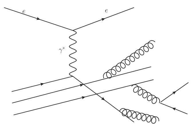
It was also seen that the scattering amplitude contained, in addition to well known kinematical factors, some structure functions $f_{p}(x)$, which depended only on the momentum $fraction$ $x\equiv p_{part}/p_{proton}=(-q^{2})/(2M_{p}\nu)$, of the partons (quarks). Here $\nu=E_{e}-{E_{e}}^{{}^{\prime}}$ is the energy difference between the in- and out going electrons.

The intepretation of data is the following: At high energies, the proton consist of “sea-quarks” = quarks and anti-quarks and gluons in addition to the three valence quarks $(uud)$ forming the proton. In other words, the proton contains the (usual) three valence quaks for small energies plus some gluons plus some quark anti-quark pairs when the energy grows. The quarks cannot be kicked out of the proton. The energy from the colliding electron (transmitted via the virtual photon) is used to make a quark anti-quark pair. Then for a (very) short time the proton contains four quarks and an anti-quark, which combine to one baryon and one meson. The quark anti-quark pair is thought to be made via the emission of a gluon which again makes the quark anti-quark pair. This gluon is the analogue of the photon in elecromagnetic interactions, where a photon can make an electron-positron pair.

In 1974 came the “1974-revolution”: Then the experimentalists found the socalled $\Psi$-particles. The decay-spectrum of these particles behaved qualitatively like the decay-spectrum of positronium $e^{+}\,e^{-}$. The $\Psi$ particles were intepreted as a system of a heavy (for that time) particle (quark) $c$ and its anti-particle $\bar{c}$. In other words $\Psi=(c\bar{c})$. After these discoveries, the quark picture was accepted among (almost) all particle physicists.

Before the quark picture was accepted, strong interactions meant nuclear forces. Now we might look slightly different about this.

Two protons will repel each other electrically. But if they come very close the may attract each other because the color forces are stronger than the electric ones at very close distance. Two protons will feel the “tail” of quark-gluon-forces, in spite of electric repulsion.
Nuclear forces are much stronger than electromagnetic forces - -when the nucleons are close to each other.

The color forces are so strong, for energies less than say 1 GeV, that the quarks can not come out of the proton.
The proton (-and the neutron) are color neutral. Now the picture is that the true strong force is the color force, while the nuclear force is only the tail of the color force, some times called the deduced color force. The color force binds quarks together to baryons and mesons, while the nuclear force bind nucleons to various clusters of nucleons, i.e. nuclei.

What is strange about the color force is that it is relatively weak for high energies (corresponding to short distances) while it is extremely strong at long distanes (energies of about say hundred of MeV and smaller). When quarks were established there was a good candidate for a field theory for the color force, namely the Yang Mills theory.

Assuming that quarks exsist and carry three different colors, one may write down a quark gluon field theory of Yang-Mills theory type with gauge group $SU(3)_{c}$, where the subscript $c$ stands for color. Thus QCD has the form

$\displaystyle{\cal L}_{QCD}\,=\,\sum_{q}\overline{q}\,\gamma^{\mu}\,\left(i\partial_{\mu}\,-\,g_{s}t^{a}\,A_{\mu}^{a}-m_{q}\right)q\,-\,\frac{1}{4}F^{a,\mu\nu}\,F^{a}_{\mu\nu}$

(37)

Note that there is a sum over quark flavors $q=u,d,s,...$, and that the gluons are the same for all flavors !. The field tensor has an extra term, as all YM theories, see (36):

$$F^{a}_{\mu\nu}\,=\,(\partial_{\mu}A^{a}_{\nu}\,-\,\partial_{\nu}A^{a}_{\mu})\,+\,g_{s}\,f^{abc}A^{b}_{\nu}A^{c}_{\nu}\;,$$

(38)

where $A^{a}_{\mu}$ are the eight gluon four vector fields ($a=1,2,..8$ and $\mu=0,1,2,3$). The symbol $q$ is now very compact. All the six quark fields $q$ ($q=u,d,s,c,b,t)$ have $3$ different color components (one Dirac field per color, and all Dirac fields have four components). Thus the quark field $q$ has in total $6\times 3\times 4$ components. The $t^{a}$ matrices are generators ($3\times 3$-matrices) of the gauge group $SU(3)_{c}$. It is important that the gluons interact among themselves! We obtain triple and quartic vertices. The existence of this triple gluon vertex has dramatic consequences for QCD compared to QED.

QCD is significantly different from QED due to the triplet gluon coupling The copling $g_{s}$ is universal, the same for quark-gluon and triple gluon couplings. This is a consequence og gauge invariance. It is found that perturbative QCD breaks down for low energies (say 1-2 GeV. See later).

Both in QED and Yang Mills theory (-and thereby QCD) an important ingredience is gauge invariance.

The gauge transformations in QED are

$\displaystyle\psi(x)\;\rightarrow\;\psi(x)^{\prime}\,=\,e^{i\alpha(x)}\,\,\psi(x)\;,\,A_{\mu}(x)\rightarrow A_{\mu}(x)^{\prime}\,=\,A_{\mu}(x)\,-\,\frac{1}{e}\,\partial_{\mu}\alpha(x)\;.$

(39)

Under these combined transformations the QED Lagrangian given by (19) - (22) is invariant.

For Yang-Mills theory the corresponding transformation for fermion fields is

$\displaystyle f(x)\;\rightarrow\;f(x)^{\prime}\,=\;U(x)\,f(x)\quad;\;\,U(x)\,\in\,SU(n)\;(-\mbox{for instance})\;.$

(40)

Gauge field transformations in the non-Abelian has to be such that $D_{\mu}f$ tansforms as $f$:

$$iD_{\mu}f\;\rightarrow iD^{\prime}_{\mu}f^{\prime}\,=U\,iD_{\mu}f\;.$$

(41)

To obtain this the transformation must contain a rotation among fields:

$$A_{\mu}\,\,\rightarrow A_{\mu}^{\prime}\;=\;U\,A_{\mu}\,U^{\dagger}\;+\;\frac{i}{g}\,\left(\partial_{\mu}U\right)\,U^{\dagger},$$

(42)

and

$$F_{\mu\nu}\,\rightarrow\,F_{\mu\nu}^{\prime}\;=\;U\,F_{\mu\nu}\,U^{\dagger}\;\,;\mbox{where}\;\,U\,=\,U(x)\,=\,e^{it^{a}\alpha^{a}(x)}\;,$$

(43)

where $\alpha^{a}(x)$ is a set of real functions. Here $A(x)_{\mu}\equiv t^{a}A(x)_{\mu}^{a}\,$, and similarly we define $F(x)_{\mu\nu}\equiv t^{a}F(x)_{\mu\nu}^{a}$.

Early in the 1950’s before I enteed university physics, one discussed the “$\theta-\tau$-puzzle”: The experimentalists found apparently two different particles $\theta$ and $\tau$ with the same mass. The $\theta$ decayed to two pions ($\pi$-mesons), and $\tau$ deayed to 3 pions. $\theta$ and $\tau$ was thought to be different because a system of two pions has different parity compared to a system of three pions. Now Lee and Yang explained in 1956 that the solution to the puzzle is that parity is a broken symmetry in weak interactions and that $\theta$ and $\tau$ is actually the same particle, namely the kaon ($K$-meson), which could decay both to two or three pions. The $\pi$’s and $K$’s are pseudo-scalar particles, that is, thay have spin zero and intrinsic parity minus ($0^{-}$).

The most known weak process is probably $\beta$-decay :

$$n\rightarrow p\,e^{-}\;\overline{\nu_{e}}\;,$$

(53)

which may occurr for free neutrons or for neutrons bound in a nucleus. The process is famous because of the $C-14$ age test. A free neutron has an average life time of order 15 minutes. For a bound neutron it depends on the nucleus. In many cases it is stable, and is not a $\beta$-emitter. In a few nuclei the bound proton might decay (they are positron emitters) and we have the inverse process:

$$p\rightarrow n\,e^{+}\nu_{e}\;.$$

(54)

This cannot occurr for free protons because the proton is lighther than the neutron. The process (54) is used in PET-scanners in hospitals. The process(53) and (54) also breaks parity-symmetry.

The charged $\pi$’s and $K$’s could also decay to leptons, for instance

$$\pi^{+},K^{+}\rightarrow\mu^{+}\nu_{\mu}\;\,\mbox{or}\;\,e^{+}\nu_{e}\;.$$

(55)

Here the decays to the heavier lepton $\mu$ is most probable. As a curiocity: When the muon was discovered one physicist said: “Who ordered that”. He meant it was “no need” for it. However, it is useful because then pions from cosmic radiation decay faster than if the electron were the only charged lepton. With only the electron we would get more pions in our heads!

For massive fermions and anti-fermions there are in total four degrees of freedom. BUT: For massless fermions/anti-fermions there are in total only two degrees of freedom Then one makes the following definitions:

Neutrinos are considered to be lefthanded particles $(\nu_{e})_{L}$, and and antineutrinos as righthanded antiparticles $(\overline{\nu_{e}})_{R}$. Then one defined the leptoic charges for the electron, the muon ($\mu$) and their neutrinos.Then one has:

• •

  Lepton number $L_{e}$ is conserved:
  $L(e^{-})\,=\,L(\nu_{e})=\,+1$ and $L(e^{+})\,=\,L(\overline{\nu_{e}})=\,-1$

• •

  Lepton number $L_{\mu}$ conserved:
  $L(\mu^{-})\,=\,L(\nu_{\mu})=\,+1$ and $L(\mu^{+})\,=\,L(\overline{\nu_{\mu}})=\,-1$
  (Similar for $L_{\tau}$)

such that $L_{e}$ and $L_{\mu}$ was (so far) conserved. Thus one had conservation of lepton numbers built into the theory ! -as visible in the pure leptonic decay mode

$$\mu^{-}\rightarrow\,e^{-}\overline{\nu_{e}}\,\nu_{\mu}\;.$$

(56)

In the early 1960’s there were no theory for weak interactions like QED for the electromagnetic interactions. But already in the 1930-ties Fermi wrote down an effective interaction for four fermion fields acting in a point. Thought as an interaction Lagrangian, the Fermi interaction contained a product of the neutron field $\psi_{n}$, the (adjoint of) the proton field $\psi_{p}$ the electron field $\psi_{e}$ and the (adjoint of) the neutrino field $\psi_{\nu}$. But was the fields combined into vectors (as in QED), or was it scalars, or tensors? Little was from the beginning known about the interaction, except for its strength, the Fermi constant

$$G_{F}\simeq\frac{10^{-5}}{m_{p}^{2}}\;\,.$$

(57)

Later, in 1958 Feynman and Gell-Mann showed Feynman:1958ty that the interaction could be written as a product of two left-handed currents

$${\cal L}_{F}\,=\,4\frac{G_{F}}{\sqrt{2}}\,j(W,N)^{\mu}\,j(W,l)_{\mu}\;,\quad$$

(58)

where the weak currents are left-handed,- i.e a vector current minus an axial current divided by 2:

$$j(W)_{\mu}\,=\,\frac{1}{2}\left(j^{V}_{\mu}\,-\,j^{A}_{\mu}\right)\,.$$

(59)

In beta-decay the nucleonic (N) and an leptonic (l) currents can be written

$$j(W,N)^{\mu}=\frac{1}{2}\overline{\psi_{p}}\gamma^{\mu}(1-\gamma_{5})\psi_{n}\;\;\;\,,\;\,\mbox{and}\;\,j(W,l)^{\mu}=\frac{1}{2}\overline{\psi_{e}}\gamma^{\mu}(1-\gamma_{5})\psi_{\nu_{e}}\,\;,$$

(60)

respectively. The $\psi$’s are the various particle fields in a self-explained way. Note that $j^{A}_{\mu}\,=\,\overline{\psi}\,\gamma_{\mu}\,\gamma_{5}\,\psi$, such that the left-handed current may be written:

$$j(W)_{\mu}\,=\psi\gamma_{\mu}\,P_{L}\,\psi\;,\quad P_{L,R}\,\equiv\,\frac{1}{2}\,\left(1\,\mp\,\gamma_{5}\,\right)$$

(61)

where $P_{L,R}$ are the left and right projectors in Dirac space:

$$(P_{L})^{2}\,=\,P_{L}\;,\;\,(P_{R})^{2}\,=\,P_{R}\;,\;P_{L}\cdot P_{R}\,=\,P_{R}\,\cdot P_{L}\,=0\,,P_{L}\,+\,P_{R}\,=\,1\;.$$

(62)

A Dirac field can be split in two parts:

$$\psi\,=\,\psi_{L}\,+\psi_{R}\;,\;\psi_{L}\,=\,P_{L}\,\psi\;,\;\psi_{R}\,=\,P_{R}\,\psi\;,$$

(63)

where $\psi_{L}$ = left spinning (left screw)particle. and $\psi_{R}$ = right spinning (right screw) particle. In this way parity violation is built into the theory. Note that if the neutrino $\nu_{e}$ is purely lefthanded, then the apparent vector current for $\nu_{e}\rightarrow e^{-}$ is automatically lefthanded:

$$j(W,e)_{\mu}\,=\,\overline{\psi_{e}}\,\gamma_{\mu}\,\psi_{\nu_{e}}\;=\,\overline{\psi_{e}}\,\gamma_{\mu}\,(\psi_{\nu_{e}})_{L}\;=\,\overline{\psi_{e}}\,\gamma_{\mu}\,P_{L}\psi_{\nu_{e}}\;.$$

(64)

Note that $\overline{\psi_{L}}=(P_{L}\psi)^{\dagger}\gamma_{0}=\overline{\psi}\,P_{R}$, such that:

$$\overline{\psi_{L}}\,\gamma_{\mu}\,\psi_{L}\,=\,\overline{\psi}\,\gamma_{\mu}\,P_{L}\psi\;\,,\;\,\overline{\psi_{R}}\,\gamma_{\mu}\,\psi_{R}\,=\,\overline{\psi}\,\gamma_{\mu}\,P_{R}\psi\;\,,\;\;\overline{\psi}\,\psi\,=\,\overline{\psi_{L}}\,\psi_{R}\,\,+\,\overline{\psi_{R}}\,\psi_{L}\;.$$

(65)

From the last equation we observe that mass terms mixes left and right fields. We observe that symbolically for a product of lefthanded currents:

$$(V-A)^{2}\;=\;(V\,V\,+A\,A)\;-\;(V\,A\,+A\,V)\;,$$

(66)

where the last term violates parity !

If the two currents were mediated by a heavy weak boson $W$ coupling to with strength $g_{W}$, then one would have

$$\,-\,4\frac{G_{F}}{\sqrt{2}}\;\,\rightarrow\;\,\frac{g_{W}^{2}}{q^{2}-M_{W}^{2}}\,.$$

(67)

If the four momentum $q$ is small compared to $M_{W}$; i.e $|q^{2}|<<M_{W}^{2}$, then

$$4\frac{G_{F}}{\sqrt{2}}\,=\,\frac{g_{W}^{2}}{M_{W}^{2}}\;.$$

(68)

There existed an hypothes already in the 1930’s that weak interactions were mediated by a massive boson $W$. But at that time the $W$ was very hypothetic, and how massive it should be was not known. (its spin was also not clear). But if one assumed that $g_{W}$ were of the same order of magnitude as the electric charge $e$, one could deduce from the measured value of $G_{F}$, that the mass of the $W$ would be of the order 40 proton masses, which turned up to be correct up to a factor 2.

References

- [1] R.P. Feynman, Phys. Rev. 76 (1949) 749-759
- [2] J.D. Bjorken, D.D. Drell, Relativistic quantum mechanics, isbn = ”978-0-07-005493-6” Published by McGraw-Hill”, (year 1965)
- [3] T. Regge, Tullio and M. Verde, Il Nuovo Cimento 10 (1953), 997-1011
- [4] Murray Gell-Mann, report Number CTSL-20, TID-12608 (1961), doi = ”10.2172/4008239”,
- [5] TD Lee, and C.N. Yang, Phys.Rev. (!956) 104 (1956) 254-258
- [6] C.N. Yang and R.L. Mills, Phys. Rev. 96 (1954), 191-195.
- [7] R.P. Feynman, and M. Gell-Mann, Phys.Rev. 109 (1958) 193
- [8] J.H. Christenson, J.W. Cronin, V.L. Fitch, and R. Turlay, Phys. Rev. Lett. 13 (1964) 138-140
- [9] S. Weinberg, PhysRevLett 19 (1967) 1264-1266
- [10] P.W. Higgs, Phys.Rev.Lett. 13 (1964) 508-509
- [11] N. Cabibbo, PhysRevLett10 (1963) 531
- [12] S.L. Glashow, S. L., J. Iliopoulos, and L. Maiani, PhysRevD2 (1970) 1285
- [13] M. Kobayashi and T. Maskawa, Prog. Theor. Phys. 49 (1973) 652-657
- [14] J.O.Eeg, Nucl. Phys. B Proc. Suppl 7 (1989) 129-148