Quantum matrix geometry in the lowest Landau level and higher Landau levels

The non-commutative geometry is a promising mathematical framework for describing a quantized space-time. Typical and well-studied examples of the non-commutative spaces are non-commutative plane, fuzzy sphere and fuzzy hyperboloid. They exhibit mathematically unique structures and also exemplify solutions of the Matrix models of string theory.

Usually, a non-commutative structure is postulated when defining models such as in the non-commutative field theory, and their physical properties are discussed withing the given framework. Here, we will take an almost inverse approach: We will introduce Landau models at first not assuming any non-commutative structure and subsequently exploit the non-commutative structure from the models. The Landau models are simple models that describe quantum mechanics of electrons in magnetic fields. In the planar Landau model, the center-of-mass coordinates of electron are given by $X=x+i\frac{1}{B}(\partial_{y}+iA_{y})$ and $Y=y-i\frac{1}{B}(\partial_{x}+iA_{x})$ that satisfy the Heisenberg-Weyl algebra:

$$[X,Y]=i\frac{1}{B}\boldsymbol{1},~~~~~[X,\boldsymbol{1}]=[Y,\boldsymbol{1}]=0.$$

(1)

The center-of-mass coordinates obey the non-commutative algebra due to the existence of the magnetic field and the electrons behave as if they live on a non-commutative plane. As for curved non-commutative spaces, the fuzzy sphere introduced by Madore [1] (see Refs.[2, 3] also) provides a typical example. The mathematics of fuzzy two-sphere is very simple: The matrix coordinates satisfy the $SU(2)$ algebra and the sum of their squares should be a constant (times an identity matrix):

$$[X_{i},X_{j}]=i\epsilon_{ijk}X_{k},~~~~~~\sum_{i=1}^{3}X_{i}X_{i}=\text{const}\cdot\boldsymbol{1}.$$

(2)

After a few years of the work of Madore, Grosse and his collaborators succeeded to generalize the concept of the fuzzy-sphere in the four dimension [6], which is now known as the fuzzy four-sphere. The fuzzy four-sphere was rediscovered in the context of string theory and studied in detail [7, 8, 9, 10]. The fuzzy four-sphere is defined as

$$[X_{a},X_{b},X_{c},X_{d}]=\epsilon_{abcde}X_{e},~~~~~\sum_{a=1}^{5}X_{a}X_{a}=\text{const}\cdot\boldsymbol{1}.$$

(3)

Obviously, (3) is a straightforward generalization of (2) replacing the usual commutator with the Nambu four-bracket $[X_{\sigma_{1}},X_{\sigma_{2}},X_{\sigma_{3}},X_{\sigma_{4}}]\equiv\text{sgn}(\sigma)~X_{\sigma_{1}}X_{\sigma_{2}}X_{\sigma_{3}}X_{\sigma_{4}}$ [11, 12, 13]. Meanwhile, the fuzzy three-sphere [14, 15, 16, 17, 18, 19] is introduced as

$$[\![X_{\mu}X_{\nu},X_{\rho}]\!]=i\epsilon_{\mu\nu\rho\sigma}X_{\sigma},~~~~~~~\sum_{\mu=1}^{4}X_{\mu}X_{\mu}=\text{const}\cdot\boldsymbol{1}.$$

(4)

Note that, in (4), the “three bracket” $[\![X_{\mu}X_{\nu},X_{\rho}]\!]\equiv[X_{\mu},X_{\nu},X_{\rho},G_{5}]$ with $G_{5}\equiv P_{R_{+}}-P_{R_{-}}=\begin{pmatrix}1&0\\ 0&-1\end{pmatrix}$ is used.

In the following, I will discuss the Landau model realization of the fuzzy pheres.¹¹ 1 In the same spirit, the fuzzy $\mathbb{C}P^{n}$ is analyzed in [4]. See [5] as a review. Before going to details, I briefly mention the underlying idea. Suppose that we would like to construct a fuzzy manifold whose classical geometry is a coset, $M\simeq G/H$. The corresponding fuzzy manifold will be made of “quantum elements” each of which occupies some quantum finite area on $M$. As $M$ returns to itself under the transformation $G$, the set of those quantum elements should return to itself under the transformation. We may adopt the states of an irreducible representation of $G$ as such quantum elements, since irreducible representation denotes a closed set under the group transformations. Thus, the fuzzy manifold made of the states of the irreducible representation is necessarily symmetric under the transformation $G$. The stabilizer group $H$ of $M$ will be translated as the gauge group in the quantum mechanical side. In short, in passing from the classical geometry $M\simeq G/H$ to its fuzzy version $M_{F}$, we need to utilize the irreducible representations of the global symmetry group $G$ with the gauge symmetry $H$. Such a quantum mechanical model is nothing but the Landau model constructed on $M$ with the gauge symmetry $H$.

To fuzzify a two-sphere $S^{2}\simeq SO(3)/SO(2)$, we consider the Landau model with the $SO(2)\simeq U(1)$ gauge symmetry on $S^{2}$. The Landau model Hamiltonian is given by [20, 21]

$$H=-\frac{1}{2M}\sum_{i=1}^{3}(\partial_{i}+iA_{i})^{2}|_{r=\text{const}}$$

(5)

where $A_{i}$ denote the Dirac’s monopole gauge field [22]

$$A_{\mu=1,2}=-\frac{I}{2r(r+x_{3})}\epsilon_{\mu\nu}x_{\nu},~~~A_{3}=0.$$

(6)

The corresponding Landau levels are $E_{n}=\frac{1}{2M}(I(n+\frac{1}{2})+n(n+1))$ with $n=0,1,2,\cdots$ being the Landau level index, and the Landau level degeneracy is counted as $d_{n}=2n+I+1$. The $n$th Landau level eigenstates are known as the monopole harmonics $Y_{l=n+\frac{I}{2},m}^{(I/2)}(\theta,\phi)$ [20] which constitute the $SU(2)$ irreducible representation of the spin index $l=n+\frac{I}{2}$.

While there are several methods for deriving the non-commutative geometry from the Landau model, the most straightforward way is to evaluate the matrix elements of the coordinates in each Landau level:

$$(X_{i}^{(n)})_{mm^{\prime}}=\langle Y_{l,m}|x_{i}|Y_{l,m^{\prime}}\rangle|_{l=n+\frac{I}{2}}.$$

(7)

Using the formulas of the monopole harmonics, we can explicitly evaluate (7) as [23]

$$X_{i}^{(n)}=\frac{2I}{(I+2n)(I+2n+2)}S_{i}^{(l=n+\frac{I}{2})},$$

(8)

where $S^{(l)}$ denote the $SU(2)$ spin matrices with spin magnitude $l$. The $X_{i}^{(n)}$ (8) obviously satisfy the algebra of the fuzzy two-sphere (2):

$$[X_{i}^{(n)},X_{j}^{(n)}]=i\epsilon_{ijk}\frac{(I+2n)(I+2n+2)}{2I}X_{k}^{(n)},~~~~~\sum_{i=1}^{3}X_{i}^{(n)}X_{i}^{(n)}=\frac{I^{2}}{(I+2n)(I+2n+2)}\boldsymbol{1}_{2n+I+1}.$$

(9)

The $U(1)$ quantum number $m$ appears as the $2l+1$ diagonal components of $X_{z}^{(n)}~\propto~S_{z}^{(l=n+\frac{I}{2})}$ and specifies the position of the latitudes (Fig.1).

While the non-commutative structure of the lowest Landau level $(n=0)$ is usually focused in literature, the non-commutative geometry also appears in the higher Landau levels $(n\neq 0)$ as shown by (8).

Next I discuss the fuzzy four-sphere geometry. For $S^{4}\simeq SO(5)/SO(4)$, we need to consider the Landau model on $S^{4}$ in the $SO(4)$ monopole background. The $SO(4)$ group is a direct product of two $SU(2)$ groups, and then we will adopt one of them.²² 2 Recently, the author performed a full analysis for the $SO(4)$ case [24]. With the $SU(2)$ monopole gauge field [25]

$$A_{\mu=1,2,3,4}=-\frac{1}{2r(r+x_{5})}\eta_{\mu\nu}^{i}x_{\nu}S_{i}^{(I/2)},~~~A_{5}=0,~~~~~~~(\eta_{\mu\nu}^{i}=\epsilon_{\mu\nu i4}+\delta_{\mu i}\delta_{\nu 4}-\delta_{\mu 4}\delta_{\nu i}),$$

(10)

the 4D Landau Hamiltonian is constructed as [26].

$$H=-\frac{1}{2M}\sum_{a=1}^{5}{(\partial_{a}+iA_{a})}^{2}|_{r=\text{const.}}.$$

(11)

The Landau levels are given by $E_{N}=\frac{1}{2M}(I(N+1)+N(N+3))$ $(N=0,1,2,\cdots)$. The corresponding eigenstates are known as the $SU(2)$ monopole harmonics $Y_{p,q;~j,m_{j};k,m_{k}}$ [27] with the $SO(5)$ Casimir indices

$$(p,q)=(N+I,N)~~~(N=0,1,2,\cdots).$$

(12)

Note that the $SU(2)$ monopole harmonics carry the $SO(4)\simeq SU(2)\otimes SU(2)$ quantum numbers $(j,m_{j};~k,m_{k})$, which brings $D(N,I)\equiv\frac{1}{6}(N+I+2)(N+1)(2N+I+3)(I+1)$ degeneracy to the $N$th Landau level, and the $N$th Landau level eigenstates consist of $N+1$ sets of the $I+1$ $SO(4)$ irreducible representations (see Fig.2). The $SO(4)\simeq SU(2)\times SU(2)$ decomposition of the $SO(5)$ irreducible representation is given by

$$D(N,I)=\sum_{n=0}^{N}\sum_{j+k=n+\frac{I}{2}}(2j+1)(2k+1).$$

(13)

With those Landau level eigenstates, we derive the matrix coordinates

$$(X_{a}^{(N)})_{j,m_{j};k,m_{k}}=\langle Y_{N+I,N;j,m_{j};k,m_{k}}|x_{a}|Y_{N+I,N;j,m_{j};k,m_{k}}\rangle,$$

(14)

which will become $D(N,I)\times D(N,I)$ matrices.

As the last concrete example, we will discuss the fuzzy three-sphere. For $S^{3}\simeq SO(4)/SO(3)$, the corresponding Landau model is constructed on $S^{3}$ in the $SO(3)\simeq SU(2)$ monopole background. That Landau model was first analyzed in [31] and subsequently in [32, 33]. The $SU(2)$ monopole gauge field is given by

$$A_{i}=-\frac{I}{2r(r+x_{4})}\epsilon_{ijk}x_{j}S_{k}^{(I/2)},~~~A_{4}=0,$$

(17)

and the Landau Hamiltonian is

$$H=-\frac{1}{2M}\sum_{\mu=1}^{4}{(\partial_{\mu}}^{2}+iA_{\mu})|_{r=\text{const.}}.$$

(18)

The Landau levels are derived as $E_{n,s}=\frac{1}{2M}(I(n+\frac{1}{2})+n(n+2)+s^{2})$, which depend both on the Landau level index $n=0,1,2,\cdots$ and the sub-band index

$$s=\frac{I}{2},~\frac{I}{2}-1,~\frac{I}{2}-2,~\cdots,~-\frac{I}{2}.$$

(19)

The fuzzy three-sphere geometry is realized at the minimum energy level of $(n,s)=(0,1/2)$ and $(0,-1/2)$. In the lowest Landau level $(n=0)$, there are $I+1$ sub-bands [Fig.6] labeled by $s$, and the matrix coordinates of $S^{3}$ are obtained as

$$X_{\mu=1,2,3,4}=\frac{1}{I+3}\Gamma_{\mu},$$

(20)

where $\Gamma_{\mu=1,2,3,4}$ are the four matrices of (15). Aligning the fuzzy geometries in the sub-bands along the virtual 5th direction of $s$, we can reproduce the fuzzy four-sphere geometry [Fig.6] [32, 33].

Thus interestingly, the 3D Landau model “knows” the geometry of the one dimension higher Landau model. Such a hierarchical structure has been observed in the context of the fuzzy geometry [18, 19, 14, 15, 16], and the present Landau models are the physical models that nicely realize the structure.

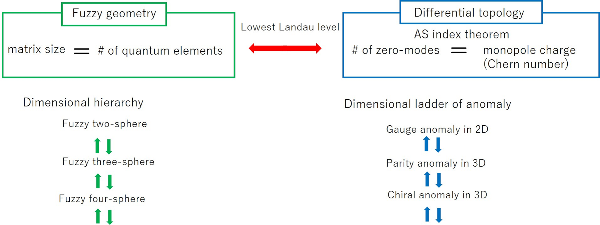
We can find a similar hierarchical structure with respect to the monopole gauge fields [28] [Fig.7]. One may wonder whether such a hierarchical relation is extended in even higher dimensions. Actually, it is straightforward to generalize the set-up of the Landau model in any dimensions, and we can show that the dimensional hierarchy ranges in all dimensions [34, 35, 36].

The dimensional hierarchy finds its origin in the differential topology. In the lowest Landau level, the degenerate eigenstates constituting the fuzzy spheres are equal to the zero-modes of the Dirac-Landau operator of the relativistic Landau models. Meanwhile, the Atiyah-Singer index theorem signifies the equality between the number of the zero-modes and the Chern number which is the monopole charge in the present Landau models [37, 35]. This implies a close relationship between the non-commutative geometry and the differential topology, since the quantum space of the fuzzy space are spanned by the zero-modes while the mathematics of the monopole gauge fields is accounted for by the fibre-bundle theory of the differential topology [36, 35]. The similar hierarchical structure in the fuzzy geometry and the monopole gauge field is a consequence of this observation. In quantum field theory, the chiral anomaly is a manifestation of the Atiyah-Singer index theorem and exhibits a hierarchical structure referred to as the dimensional ladder. The dimensional hierarchy is said to be the Landau model counterpart of the dimensional ladder of quantum anomaly [Fig.8].

Incidentally, the even D Landau models correspond to the A-class topological insulators and the odd D Landau models the AIII-class topological insulators [Fig.9]. In the topological table, it is known that there exists a dimensional relation [38, 39], which also supports the idea of the dimensional hierarchy of the Landau models.

We discussed the Landau model realization of the fuzzy spheres through the concrete evaluation of the matrix coordinates. For the 2D Landau model, the matrix geometries were identified as the fuzzy spheres in any Landau levels. Similarly for the 4D Landau model, the lowest Landau level geometry is shown to be the fuzzy four-sphere geometry. Meanwhile, the higher Landau level geometry turned out to be the nested fuzzy structure with no classical counterpart. In the 3D Landau model, the fuzzy three-sphere geometry was realized at the lowest energy level, and the hidden one dimension higher fuzzy geometry was unveiled in the lowest Landau level. The dimensional hierarchy among the Landau models is the Landau model counterpart of the dimensional ladder of quantum anomaly and implies an intimate relationship between the non-commutative geometry and the differential topology.

References

- [1] J. Madore, “The Fuzzy Sphere”, Class. Quant. Grav. 9 (1992) 69.
- [2] F. A. Berezin, “General Concept of Quantization”, Commun. math. Phys. 40 (1975) 40.
- [3] Jens Hoppe, “Quantum Theory of a Massless Relativistic Surface and a Two-dimensional Bound State Problem”, MIT PhD Thesis (1982).
- [4] D. Karabali, V. P. Nair, “Quantum Hall Effect in Higher Dimensions”, Nucl.Phys. B641 (2002) 533; hep-th/0203264.
- [5] Dimitra Karabali, V.P. Nair, S. Randjbar-Daemi “Fuzzy spaces, the M(atrix) model and the quantum Hall effect”, hep-th/0407007.
- [6] H. Grosse, C. Klimcik, P. Presnajder, “On Finite 4D Quantum Field Theory in Non-Commutative Geometry”, Commun.Math.Phys. 180 (1996) 429-438; hep-th/9602115.
- [7] Judith Castelino, Sangmin Lee, Washington Taylor, “Longitudinal 5-branes as 4-spheres in Matrix theory”, Nucl.Phys.B526 (1998) 334-350; hep-th/9712105.
- [8] P. M. Ho and S. Ramgoolam, “Higher dimensional geometries from matrix brane constructions”, Nucl.Phys.B 627 (2002) 266; hep-th/0111278.
- [9] Yusuke Kimura, “Noncommutative gauge theory on fuzzy four-sphere and matrix model”, Nucl.Phys.B 637 (2002) 177; hep-th/0204256.
- [10] Yusuke Kimura, “On higher dimensional fuzzy spherical branes”, Nucl.Phys.B 664 (2003) 512; hep-th/0301055.
- [11] Yoichiro Nambu, “Generalized Hamiltonian Dynamics”, Phys.Rev.D7 (1973) 2405-2412.
- [12] Thomas Curtright, Cosmas Zachos, “Classical and Quantum Nambu Mechanics”, Phys.Rev.D68 (2003) 085001; hep-th/0212267.
- [13] Joshua DeBellis, Christian Saemann, Richard J. Szabo, “Quantized Nambu-Poisson Manifolds and n-Lie Algebras”, J.Math.Phys.51 (2010) 122303; arXiv:1001.3275.
- [14] Z. Guralnik, S. Ramgoolam, “On the Polarization of Unstable D0-Branes into Non-Commutative Odd Spheres”, JHEP 0102 (2001) 032; hep-th/0101001.
- [15] Sanjaye Ramgoolam, “On spherical harmonics for fuzzy spheres in diverse dimensions”, Nucl.Phys. B610 (2001) 461-488; hep-th/0105006.
- [16] Sanjaye Ramgoolam, “Higher dimensional geometries related to fuzzy odd-dimensional spheres”, JHEP 0210 (2002) 064; hep-th/0207111.
- [17] Anirban Basu, Jeffrey A. Harvey, “The M2-M5 Brane System and a Generalized Nahm’s Equation”, Nucl.Phys. B713 (2005) 136-150; hep-th/0412310.
- [18] M. M. Sheikh-Jabbari, “Tiny Graviton Matrix Theory: DLCQ of IIB Plane-Wave String Theory, A Conjecture”, JHEP 0409 (2004) 017; hep-th/0406214.
- [19] M. M. Sheikh-Jabbari, M. Torabian, “Classification of All 1/2 BPS Solutions of the Tiny Graviton Matrix Theory”, JHEP 0504 (2005) 001; hep-th/0501001.
- [20] T.T. Wu, C.N. Yang, “Dirac Monopoles without Strings: Monopole Harmonics”, Nucl.Phys. B107 (1976) 1030-1033.
- [21] F.D.M. Haldane, “Fractional quantization of the Hall effect: a hierarchy of incompressible quantum fluid states", Phys. Rev. Lett. 51 (1983) 605-608.
- [22] P.A.M. Dirac, “Quantized singularities in the electromagnetic field”, Proc. Royal Soc. London, A133 (1931) 60-72.
- [23] Kazuki Hasebe, “Relativistic Landau Models and Generation of Fuzzy Spheres", Int.J.Mod.Phys.A 31 (2016) 1650117; arXiv:1511.04681.
- [24] Kazuki Hasebe, “‘SO(5) Landau Model and 4D Quantum Hall Effect in The SO(4) Monopole Background”, arXiv:2112.03038.
- [25] Chen Ning Yang, “Generalization of Dirac’s monopole to SU2 gauge fields”, J. Math. Phys. 19 (1978) 320.
- [26] S. C. Zhang and J. P. Hu, “A Four Dimensional Generalization of the Quantum Hall Effect”, Science 294 (2001) 823; cond-mat/0110572.
- [27] Chen Ning Yang, “SU(2) monopole harmonics”, J. Math. Phys. 19 (1978) 2622.
- [28] Kazuki Hasebe, “ Landau models and nested Nambu matrix geometry", Nucl.Phys. B 956 (2020) 115012; arXiv:2002.05010.
- [29] G. Ishiki, T. Matsumoto, H. Muraki, “Information metric, Berry connection, and Berezin-Toeplitz quantization for matrix geometry”, Phys. Rev. D 98 (2018) 026002; arXiv:1804.00900.
- [30] Kazuki Hasebe, in preparation.
- [31] V.P. Nair, S. Randjbar-Daemi, “Quantum Hall effect on , edge states and fuzzy ”, Nucl.Phys. B679 (2004) 447-463; hep-th/0309212.
- [32] Kazuki Hasebe, “Chiral topological insulator on Nambu 3-algebraic geometry", Nucl.Phys. B 886 (2014) 681-690; arXiv:1403.7816.
- [33] Kazuki Hasebe, “ Landau Models and Matrix Geometry”, Nucl.Phys. B 934 (2018) 149-211; arXiv:1712.07767.
- [34] K. Hasebe and Y. Kimura, “Dimensional Hierarchy in Quantum Hall Effects on Fuzzy Spheres”, Phys.Lett. B 602 (2004) 255; hep-th/0310274.
- [35] Kazuki Hasebe, “Higher Dimensional Quantum Hall Effect as A-Class Topological Insulator", Nucl.Phys. B 886 (2014) 952-1002; arXiv:1403.5066.
- [36] Kazuki Hasebe, “Higher (Odd) Dimensional Quantum Hall Effect and Extended Dimensional Hierarchy", Nucl.Phys. B 920 (2017) 475-520; arXiv:1612.05853.
- [37] Brian P. Dolan, “The Spectrum of the Dirac Operator on Coset Spaces with Homogeneous Gauge Fields”, JHEP 0305 (2003) 018; hep-th/0304037.
- [38] Shinsei Ryu, Andreas P. Schnyder, Akira Furusaki, Andreas W. W. Ludwig, “Topological insulators and superconductors: ten-fold way and dimensional hierarchy”, New J. Phys. 12 (2010) 065010; arXiv:0912.2157.
- [39] A. Kitaev, “Periodic table for topological insulators and superconductors”, Proceedings of the L.D.Landau Memorial Conference Advances in Theoretical Physics, June 22-26 (2008); arXiv:0901.2686.