跳到论文正文
W Papers独立论文阅读器 arXiv:2212.05143 论文正文 计算阅读时间 · 0%
引用这篇论文根据当前论文元数据生成,正式投稿前建议核对。


License: arXiv.org perpetual non-exclusive license
arXiv:2212.05143v1 [math.NA] 09 Dec 2022

∎

A fast convolution method for the fractional Laplacian in ℝ\mathbb{R} Thanks: This research was partially supported by the research group grant IT1615-22 funded by the Basque Government, and by the grant PID2021-126813NB-I00 funded by MCIN/AEI/10.13039/501100011033 and by “ERDF A way of making Europe”.

Jorge Cayama    Carlota María Cuesta    Francisco de la Hoz    Carlos Javier García-Cervera
Received: date / Accepted: date
Abstract

In this article, we develop a new method to approximate numerically the fractional Laplacian of functions defined on ℝ\mathbb{R}, as well as some more general singular integrals. After mapping ℝ\mathbb{R} into a finite interval, we discretize the integral operator using a modified midpoint rule. The result of this procedure can be cast as a discrete convolution, which can be evaluated efficiently using the Fast-Fourier Transform (FFT). The method provides an efficient, second order accurate, approximation to the fractional Laplacian, without the need to truncate the domain.

We first prove that the method gives a second-order approximation for the fractional Laplacian and other related singular integrals; then, we detail the implementation of the method using the fast convolution, and give numerical examples that support its efficacy and efficiency; finally, as an example of its applicability to an evolution problem, we employ the method for the discretization of the nonlocal part of the one-dimensional cubic fractional Schrödinger equation in the focusing case.

Keywords:
fractional Laplacian singular integrals numerical quadrature fast convolution fractional Schrödinger equation
MSC
26A33 35R11 65D32

1 Introduction and Preliminaries

In this paper, we develop a new method that uses the fast convolution to approximate numerically the fractional Laplacian on ℝ\mathbb{R} and some more general singular integrals. Before describing the method, let us focus on the type of operator that we want to approximate.

Among the many possible definitions of the fractional Laplacian (see, e.g., kwasnicki, where the author considers −(−Δ)α/2-(-\Delta)^{\alpha/2} with α∈(0,2)\alpha\in(0,2)), we choose (as we do in cayamacuestadelahoz2020; cayamacuestadelahoz2021):

(−Δ)α/2​u​(x)=cα​∫−∞∞u⁡(x)−u⁡(x+y)|y|1+α​𝑑y,(-\Delta)^{\alpha/2}u(x)=c_{\alpha}\int_{-\infty}^{\infty}\frac{u(x)-u(x+y)}{|y|^{1+\alpha}}dy, (1)

where α∈(0,2)\alpha\in(0,2), and

cα=α​2α−1​Γ​(1/2+α/2)π​Γ​(1−α/2);c_{\alpha}=\alpha\frac{2^{\alpha-1}\Gamma(1/2+\alpha/2)}{\sqrt{\pi}\Gamma(1-\alpha/2)};

note that all the integrals in this paper that are not absolutely convergent must be understood in the principal value sense.

Henceforth, we concentrate on applying (1) to regular functions. In particular, whenever uu is a twice continuously differentiable bounded function, i.e., u∈𝒞b2​(ℝ)u\in\mathcal{C}_{b}^{2}(\mathbb{R}), we can express (1) as (see cayamacuestadelahoz2021):

(−Δ)α/2​u​(x)=cαα​∫0∞ux​(x−y)−ux​(x+y)yα​𝑑z,(-\Delta)^{\alpha/2}u(x)=\frac{c_{\alpha}}{\alpha}\int_{0}^{\infty}\frac{u_{x}(x-y)-u_{x}(x+y)}{y^{\alpha}}dz, (2)

from which the following lemma follows.

Lemma 1 (cayamacuestadelahoz2021)

Let u∈𝒞b2​(ℝ)u\in\mathcal{C}_{b}^{2}(\mathbb{R}), then, if α∈[1,2)\alpha\in[1,2), or α∈(0,1)\alpha\in(0,1) and limx→±∞ux​(x)=0\lim_{x\to\pm\infty}u_{x}(x)=0,

(−Δ)α/2u(x)={1π​∫−∞∞ux​(y)x−y​dy,if α=1,cαα⁡(1−α)​∫−∞∞ux​x​(y)|x−y|α−1​dy,if α≠1.(-\Delta)^{\alpha/2}u(x)=\left\{\begin{aligned} &\frac{1}{\pi}\int_{-\infty}^{\infty}\frac{u_{x}(y)}{x-y}dy,&&\text{if $\alpha=1$},\\ &\frac{c_{\alpha}}{\alpha(1-\alpha)}\int_{-\infty}^{\infty}\frac{u_{xx}(y)}{|x-y|^{\alpha-1}}dy,&&\text{if $\alpha\neq 1$}.\end{aligned}\right. (3)

In this paper, we work with (3), rather than with (1). Note that, in this form, it is obvious that, when α=1\alpha=1, the fractional Laplacian is just the Hilbert transform of the derivative of u⁡(x)u(x), i.e., (−Δ)1/2​u​(x)≡ℋ⁡(ux​(x))(-\Delta)^{1/2}u(x)\equiv\mathcal{H}(u_{x}(x)). Since the numerical computation of the Hilbert transform has long been studied (see, e.g., weideman1995), we have limited ourselves to considering the case α≠1\alpha\not=1 in this paper.

One of the main difficulties in the computation of the fractional Laplacian is dealing with the unboundedness of ℝ\mathbb{R}. In this paper, we follow the approach in delahozcuesta2016; cayamacuestadelahoz2020; cayamacuestadelahoz2021, i.e., we map ℝ\mathbb{R} into a bounded interval, by means of an algebraic map (see Boyd1987):

ξ=xL2+x2∈[−1,1]⟺x=L​ξ1−ξ2∈ℝ,\xi=\frac{x}{\sqrt{L^{2}+x^{2}}}\in[-1,1]\Longleftrightarrow x=\frac{L\xi}{\sqrt{1-\xi^{2}}}\in\mathbb{R},

with L>0L>0. Then, we consider another change of variable:

x=L​cot⁡(s)∈ℝ⟺ξ=cos⁡(s)∈[−1,1]⟺s=arccos⁡(ξ)∈[0,π],x=L\cot(s)\in\mathbb{R}\Longleftrightarrow\xi=\cos(s)\in[-1,1]\Longleftrightarrow s=\arccos(\xi)\in[0,\pi], (4)

so we need to express (3) in terms of s∈[0,π]s\in[0,\pi], for which we use d​x=−L​sin−2⁡(s)​d​sdx=-L\sin^{-2}(s)ds, together with the following identities (see Boyd1987):

ux​(x)=−sin2⁡(s)L​us​(s),ux​x​(x)=sin4⁡(s)L2​us​s​(s)+2​sin3⁡(s)​cos⁡(s)L2​us​(s),u_{x}(x)=-\frac{\sin^{2}(s)}{L}u_{s}(s),\qquad u_{xx}(x)=\frac{\sin^{4}(s)}{L^{2}}u_{ss}(s)+\frac{2\sin^{3}(s)\cos(s)}{L^{2}}u_{s}(s),

where, with some abuse of notation, u⁡(s)≡u⁡(x⁡(s))u(s)\equiv u(x(s)). Then, (3) becomes (see cayamacuestadelahoz2021):

(−Δ)α/2u(s)={sin⁡(s)L​π​∫0πsin⁡(η)​us​(η)sin⁡(s−η)​dη,if α=1,cα​|sin⁡(s)|α−1Lα​α​(1−α)⋅∫0πsinα⁡(η)​(sin⁡(η)​us​s​(η)+2​cos⁡(η)​us​(η))|sin⁡(s−η)|α−1​dη,if α≠1,(-\Delta)^{\alpha/2}u(s)=\left\{\begin{aligned} &\frac{\sin(s)}{L\pi}\int_{0}^{\pi}\frac{\sin(\eta)u_{s}(\eta)}{\sin(s-\eta)}d\eta,&&\text{if $\alpha=1$},\\ &\frac{c_{\alpha}|\sin(s)|^{\alpha-1}}{L^{\alpha}\alpha(1-\alpha)}\\ &\quad\cdot\int_{0}^{\pi}\frac{\sin^{\alpha}(\eta)(\sin(\eta)u_{ss}(\eta)+2\cos(\eta)u_{s}(\eta))}{|\sin(s-\eta)|^{\alpha-1}}d\eta,&&\text{if $\alpha\neq 1$},\end{aligned}\right. (5)

where, again abusing notation, we use (−Δ)α/2(-\Delta)^{\alpha/2} for the resulting operator in the variable ss. The structure of (5) strongly suggests considering a Fourier series expansion of u⁡(s)u(s):

u⁡(s)=∑k=−∞∞u^​(k)​ei​k​s,u(s)=\sum_{k=-\infty}^{\infty}\hat{u}(k)e^{iks},

and precisely this approach was followed in cayamacuestadelahoz2021, where a pseudospectral method was proposed to approximate numerically (5), for which a fast and accurate numerical approximation of (−Δ)α/2​ei​n​s(-\Delta)^{\alpha/2}e^{ins}, with n∈ℤn\in\mathbb{Z}, was necessary. On the other hand, in cayamacuestadelahoz2020, (−Δ)α/2​ei​2​n​s(-\Delta)^{\alpha/2}e^{i2ns} was expressed in terms of the hypergeometric function F12{}_{2}F_{1}. In fact, there are more results in this direction, like in Sheng2020, where the nn-dimensional fractional Laplacian of different sets of functions was expressed in terms of hypergeometric functions.

However, in the current paper, we follow a different approach, namely, we consider a second-order modification of the midpoint rule applied to (5) that, combined with a fast Fourier transform (FFT) based convolution algorithm (see, e.g., Garcia-Cervera2007), yields a fast method that allows considering very large numbers of points without the need of evaluating hypergeometric functions. Indeed, some of the commercially available implementations of the hypergeometric functions can be numerically inefficient, and, in some cases even inaccurate (see cayamacuestadelahoz2020 for a discussion on this, and how the use of variable precision arithmetic may be required).

There is a wide range of publications related to the effectiveness of different methods to solve numerically nonlocal fractional operators. For instance, there are schemes using a finite-difference approximation, such as TianDu2013; Gao2014; DuoWykZhang2018, and HuangOberman2014; HuangOberman2016; MindenYing2018; DuoZhang2019; the latter schemes are based on singularity subtraction and finite-difference approximation by applying a quadrature rule in a bounded domain. There are also algorithms based on the Caffarelli-Silvestre extension CaffarelliSilvestre2007; HuLiLi2017; Nochetto2015, followed by the application of spectral approaches AcostaBorthagaray2016; MaoKarniadakis2018; ZayernouriKarniadakis2014. A more recent publication is, for instance, ChenShen2020, where a fast spectral Galerkin method using the generalized Laguerre functions for the extension problem is applied. A description of some of these techniques can be found in the recent review article DElia:2020.

All these publications have in common the use of truncation in the integration domain (which leads to a natural deterioration of the rate of convergence), or that they solve problems on a bounded domain where different definitions of the fractional Laplacian are not equivalent (see, e.g., the introduction of bonfortevazquez2016 and the references therein); therefore, in order to make a fair comparison of the method in this paper, we must do it with those methods that do not truncate the domain. In this regard, with respect to cayamacuestadelahoz2021, the method presented here is capable of working with much larger amounts of points (and it does it very efficiently); and with respect to cayamacuestadelahoz2020, which relies on the expression of the fractional Laplacian in terms of bases of functions defined on ℝ\mathbb{R} using hypergeometric functions (see also Sheng2020), the current approach avoids the evaluation of those functions, which is numerically expensive and potentially inaccurate.

This article is organized as follows: In Section 2, we introduce the quadrature formula used in this paper, and prove rigorously its order of convergence. This might seem not necessary, given that there are classical results regarding standard quadrature methods for singular integrals (see, e.g., Lyness1967; waterman64; navot61; kapur.rokhlin:1997), but we remark that none of these apply directly to the particular quadrature presented here. It might be possible to get the same results by adapting the general method presented in, e.g., Lyness1967 to our quadrature, but this computation seems more cumbersome than getting the error estimates directly, and thus, we opted for the latter. In Section 3, based on that quadrature formula, we develop a second-order method to approximate numerically the fractional Laplacian for α≠1\alpha\not=1. In fact, we approximate the more general singular integral:

I⁡(s)=∫0πsinβ⁡(η)​|sin⁡(η−s)|γ​f​(η)​𝑑η,I(s)=\int_{0}^{\pi}\sin^{\beta}(\eta)|\sin(\eta-s)|^{\gamma}f(\eta)d\eta, (6)

where β>0\beta>0, γ>−1\gamma>-1. The main result in this section is Theorem 3.1, in which we show that the proposed method approximates integral (6) to second order accuracy. In Section 4, we explain the fast convolution algorithm (that we will refer to as fast convolution) applied to (6), which yields an efficient evaluation of the numerical quadrature used to approximate the fractional Laplacian. In Section 5, we detail how to implement the method in Matlab matlab. In Section 6, we carry out the numerical experiments; in particular, we simulate the fractional cubic nonlinear Schrödinger equation in the focusing case.

All the simulations have been run in an Apple MacBook Pro (13-inch, 2020, 2.3 GHz Quad-Core Intel Core i7, 32 GB).

2 A modified midpoint rule

Let f∈𝒞2​[a,b]f\in\mathcal{C}^{2}[a,b], N∈ℕN\in\mathbb{N}, h=(b−a)/Nh=(b-a)/N, and denote xn=a+h​nx_{n}=a+hn, xn+1/2=a+h⁡(n+1/2)x_{n+1/2}=a+h(n+1/2) and xn+1=a+hx_{n+1}=a+h (in general, in this paper, if g⁡(n)g(n) is an expression depending on nn, we denote xg⁡(n)≡a+g⁡(n)​hx_{g(n)}\equiv a+g(n)h, or, when a=0a=0, xg⁡(n)≡g⁡(n)​hx_{g(n)}\equiv g(n)h); then, the well-known midpoint rule satisfies (see, e.g., Quarteroni2007):

∫xnxn+1f⁡(x)​𝑑x−h​f​(xn+1/2)=(xn+1−xn)324​f′′​(ξn),ξn∈(xn,xn+1),\int_{x_{n}}^{x_{n+1}}f(x)dx-hf(x_{n+1/2})=\frac{(x_{n+1}-x_{n})^{3}}{24}f^{\prime\prime}(\xi_{n}),\quad\xi_{n}\in(x_{n},x_{n+1}), (7)

and, hence,

∫abf⁡(x)​𝑑x−h​∑n=0N−1f⁡(xn+1/2)=(b−a)324​N2​f′′​(ξ),ξ∈(a,b).\int_{a}^{b}f(x)dx-h\sum_{n=0}^{N-1}f(x_{n+1/2})=\frac{(b-a)^{3}}{24N^{2}}f^{\prime\prime}(\xi),\quad\xi\in(a,b). (8)

On the other hand, if f∉𝒞2​[a,b]f\not\in\mathcal{C}^{2}[a,b], (8) no longer holds. In particular, the study of the behavior of the midpoint rule and the trapezoidal rule to approximate numerically the integral of xβ​f​(x)x^{\beta}f(x) over intervals of the form [0,b][0,b] has long been studied (see, e.g., Lyness1967, for a very detailed exposition); for instance, if f⁡(0)≠0f(0)\not=0, and β∈(−1,0)∪(0,1)\beta\in(-1,0)\cup(0,1), there exists K>0K>0, such that

|∫0bxβ​f​(x)​𝑑x−h​∑n=0N−1xn+1/2β​f​(xn+1/2)|≤KNβ+1,\left|\int_{0}^{b}x^{\beta}f(x)dx-h\sum_{n=0}^{N-1}x_{n+1/2}^{\beta}f(x_{n+1/2})\right|\leq\frac{K}{N^{\beta+1}}, (9)

where h=b/Nh=b/N, xn+1/2=(n+1/2)​hx_{n+1/2}=(n+1/2)h. Note that we are replacing here the integrand xβ​f​(x)x^{\beta}f(x) on each subinterval [xn,xn+1][x_{n},x_{n+1}] in (9), by its value at the middle point of that interval, i.e., xn+1/2β​f​(xn+1/2)x_{n+1/2}^{\beta}f(x_{n+1/2}):

∫xnxn+1xβ​f​(x)​𝑑x≈∫xnxn+1xn+1/2β​f​(xn+1/2)​𝑑x=h​xn+1/2β​f​(xn+1/2).\int_{x_{n}}^{x_{n+1}}x^{\beta}f(x)dx\approx\int_{x_{n}}^{x_{n+1}}x_{n+1/2}^{\beta}f(x_{n+1/2})dx=hx_{n+1/2}^{\beta}f(x_{n+1/2}).

However, another option is to evaluate only f⁡(x)f(x) at x=xn+1/2x=x_{n+1/2}, and integrate exactly xβx^{\beta} over [xn,xn+1][x_{n},x_{n+1}] (when xn=0x_{n}=0, β>−1\beta>-1 must be imposed):

∫xnxn+1xβ​f​(x)​𝑑x≈∫xnxn+1xβ​f​(xn+1/2)​𝑑x=f⁡(xn+1/2)​xn+1β+1−xnβ+1β+1.\int_{x_{n}}^{x_{n+1}}x^{\beta}f(x)dx\approx\int_{x_{n}}^{x_{n+1}}x^{\beta}f(x_{n+1/2})dx=f(x_{n+1/2})\frac{x_{n+1}^{\beta+1}-x_{n}^{\beta+1}}{\beta+1}.

In fact, it is possible to consider both positive and negative values of xnx_{n} and xn+1x_{n+1}:

∫xnxn+1|x|β​f​(x)​𝑑x≈sgn⁡(xn+1)​|xn+1|β+1−sgn⁡(xn)​|xn|β+1β+1​f​(xn+1/2),\int_{x_{n}}^{x_{n+1}}|x|^{\beta}f(x)dx\approx\frac{\sgn(x_{n+1})|x_{n+1}|^{\beta+1}-\sgn(x_{n})|x_{n}|^{\beta+1}}{\beta+1}f(x_{n+1/2}), (10)

where xn+1/2=(xn+xn+1)/2x_{n+1/2}=(x_{n}+x_{n+1})/2, and if 0∈[xn,xn+1]0\in[x_{n},x_{n+1}], β>−1\beta>-1 is required.

The idea of evaluating just a part of a singular integrand at its middle point, and integrating exactly the remaining expression, is not new (see, e.g., Garcia-Cervera2007), but, to the best of our knowledge, it has not been used to approximate numerically the fractional Laplacian. In our case, the reason why (10) is preferable to the standard midpoint rule is because, unlike the latter, the former integrates exactly the singularity; moreover, the quadrature can be written as a discrete convolution, which can be evaluated efficiently with the FFT. Recall that the midpoint rule, the trapezoidal rule and other quadrature rules lose accuracy in the presence of singularities, so by integrating the singularities exactly, there is an improvement with respect to (9), as we show in the following result.

Theorem 2.1

Let f∈𝒞2​[a,b]f\in\mathcal{C}^{2}[a,b], where 0≤a<b0\leq a<b, and let β≠−1\beta\not=-1 (additionally, β>−1\beta>-1 is required when a=0a=0), N∈ℕN\in\mathbb{N}, h=(b−a)/Nh=(b-a)/N, xn=a+h​nx_{n}=a+hn, etc. Define

E=∫abxβ​f​(x)​𝑑x−∑n=0N−1xn+1β+1−xnβ+1β+1​f​(xn+1/2).E=\int_{a}^{b}x^{\beta}f(x)dx-\sum_{n=0}^{N-1}\frac{x_{n+1}^{\beta+1}-x_{n}^{\beta+1}}{\beta+1}f(x_{n+1/2}). (11)

Then, there exists K>0K>0, such that

|E|≤{KN2,if a>0,KN2,if a=0 and β≥0,KN2,if a=0 and β∈(−1,0) and f′​(0)=0,KN2+β,if a=0 and β∈(−1,0) and f′​(0)≠0.|E|\leq\left\{\begin{aligned} &\frac{K}{N^{2}},&&\text{if $a>0$},\\ &\frac{K}{N^{2}},&&\text{if $a=0$ and $\beta\geq 0$},\\ &\frac{K}{N^{2}},&&\text{if $a=0$ and $\beta\in(-1,0)$ and $f^{\prime}(0)=0$},\\ &\frac{K}{N^{2+\beta}},&&\text{if $a=0$ and $\beta\in(-1,0)$ and $f^{\prime}(0)\not=0$}.\end{aligned}\right. (12)

In the rest of this section, we will prove Theorem 2.1, for which we need a number of auxiliary results.

2.1 Some auxiliary results

Suppose that β∉ℕ∪{0}\beta\not\in\mathbb{N}\cup\{0\}; then, according to the well-known Newton’s generalized binomial theorem,

(1+x)β=∑n=0∞(βn)​xn,(1+x)^{\beta}=\sum_{n=0}^{\infty}\binom{\beta}{n}x^{n}, (13)

where 00≡10^{0}\equiv 1. Note that, when β∈ℕ∪{0}\beta\in\mathbb{N}\cup\{0\}, we have the standard binomial theorem. We recall two important properties of the binomial coefficients, for n∈ℕn\in\mathbb{N}:

(βn)≡βn​(β−1n−1),(βn)≡(β−1n)+(β−1n−1).\binom{\beta}{n}\equiv\frac{\beta}{n}\binom{\beta-1}{n-1},\qquad\binom{\beta}{n}\equiv\binom{\beta-1}{n}+\binom{\beta-1}{n-1}.

On the other hand, in (13), it is immediate to check that the infinite sum is absolutely convergent for |x|<1|x|<1, and, if additionally β>0\beta>0, then it is also absolutely convergent when |x|=1|x|=1; this can be checked, e.g., by applying the well-known D’Alembert and Raabe criteria, respectively. In this paper, all the infinite sums of functions appearing are absolutely convergent for the considered parameters and values of xx (which can be checked by using those criteria or any other), and hence, their terms can be freely reordered, etc. In particular, we will use the following consequence of Newton’s generalized binomial theorem:

(1+x)β−(1−x)ββ\displaystyle\frac{(1+x)^{\beta}-(1-x)^{\beta}}{\beta} =1β​[∑n=0∞(βn)​xn−∑n=0∞(βn)​(−1)n​xn]=2β​∑n=0∞(β2​n+1)​x2​n+1\displaystyle=\frac{1}{\beta}\left[\sum_{n=0}^{\infty}\binom{\beta}{n}x^{n}-\sum_{n=0}^{\infty}\binom{\beta}{n}(-1)^{n}x^{n}\right]=\frac{2}{\beta}\sum_{n=0}^{\infty}\binom{\beta}{2n+1}x^{2n+1} (14)
=∑n=0∞22​n+1​(β−12​n)​x2​n+1.\displaystyle=\sum_{n=0}^{\infty}\frac{2}{2n+1}\binom{\beta-1}{2n}x^{2n+1}. (15)

We also need the following property of the generalized binomial coefficients.

Lemma 2

Let m,l∈ℕ∪{0}m,l\in\mathbb{N}\cup\{0\}, then

∑k=0m(−1)m−k(mk)(β+kl)={(βl−m),if l≥m,0,if l<m.\sum_{k=0}^{m}(-1)^{m-k}\binom{m}{k}\binom{\beta+k}{l}=\left\{\begin{aligned} &\binom{\beta}{l-m},&&\text{if $l\geq m$},\cr&0,&&\text{if $l<m$}.\end{aligned}\right. (16)
Proof

We use an induction argument. When m=0m=0, (16) is trivially true:

∑k=00(−1)0−k​(0k)​(β+kl)=(βl).\sum_{k=0}^{0}(-1)^{0-k}\binom{0}{k}\binom{\beta+k}{l}=\binom{\beta}{l}.

Suppose now that (16) holds until a certain m∈ℕm\in\mathbb{N}. We will prove it for m=m+1m=m+1:

∑k=0m+1(−1)m+1−k​(m+1k)​(β+kl)=∑k=1m+1(−1)m+1−k​(mk−1)​(β+kl)\displaystyle\sum_{k=0}^{m+1}(-1)^{m+1-k}\binom{m+1}{k}\binom{\beta+k}{l}=\sum_{k=1}^{m+1}(-1)^{m+1-k}\binom{m}{k-1}\binom{\beta+k}{l}
+∑k=0m(−1)m+1−k(mk)(β+kl)\displaystyle\quad\qquad+\sum_{k=0}^{m}(-1)^{m+1-k}\binom{m}{k}\binom{\beta+k}{l}
=∑k=0m(−1)m−k​(mk)​((β+1)+kl)−∑k=0m(−1)m−k​(mk)​(β+kl)\displaystyle\quad=\sum_{k=0}^{m}(-1)^{m-k}\binom{m}{k}\binom{(\beta+1)+k}{l}-\sum_{k=0}^{m}(-1)^{m-k}\binom{m}{k}\binom{\beta+k}{l}
={(β+1l−m)−(βl−m)=(βl−(m+1)),if l≥m+1,(β+1l−m)−(βl−m)=(β+10)−(β0)=1−1=0,if l=m,0−0=0,if l<m,\displaystyle\quad=\left\{\begin{aligned} &\binom{\beta+1}{l-m}-\binom{\beta}{l-m}=\binom{\beta}{l-(m+1)},&&\text{if $l\geq m+1$},\cr&\binom{\beta+1}{l-m}-\binom{\beta}{l-m}=\binom{\beta+1}{0}-\binom{\beta}{0}=1-1=0,&&\text{if $l=m$},\cr&0-0=0,&&\text{if $l<m$},\end{aligned}\right.

where we have divided the case l<m+1l<m+1 in two cases, l=ml=m and l<ml<m. ∎

At its turn, Lemma 2 is needed to prove the following result.

Lemma 3

Let β≠−1\beta\not=-1, m∈ℕ∪{0}m\in\mathbb{N}\cup\{0\}, a≥0a\geq 0, h>0h>0, n∈ℕ∪{0}n\in\mathbb{N}\cup\{0\} (additionally, β>−1\beta>-1 is required, when both a=0a=0 and n=0n=0), xn=a+n​hx_{n}=a+nh, etc., then

∫xnxn+1xβ(x−xn+1/2)mdx={∑l=0∞h2​l+m+122​l+m​(2​l+m+1)​(β2​l)​xn+1/2β−2​l,m≡0mod2,∑l=0∞h2​l+m+222​l+m+1​(2​l+m+2)​(β2​l+1)​xn+1/2β−2​l−1,m≡1mod2.\displaystyle\int_{x_{n}}^{x_{n+1}}x^{\beta}(x-x_{n+1/2})^{m}dx=\left\{\begin{aligned} &\sum_{l=0}^{\infty}\frac{h^{2l+m+1}}{2^{2l+m}(2l+m+1)}\binom{\beta}{2l}x_{n+1/2}^{\beta-2l},&&m\equiv 0\bmod 2,\cr&\sum_{l=0}^{\infty}\frac{h^{2l+m+2}}{2^{2l+m+1}(2l+m+2)}\binom{\beta}{2l+1}x_{n+1/2}^{\beta-2l-1},&&m\equiv 1\bmod 2.\end{aligned}\right. (17)
Proof

In order to compute the integral, we expand (x−xn+1/2)m(x-x_{n+1/2})^{m} by means of Newton’s binomial:

∫xnxn+1\displaystyle\int_{x_{n}}^{x_{n+1}} xβ​(x−xn+1/2)m​𝑑x=∑k=0m(mk)​(−xn+1/2)m−k​∫xnxn+1xβ+k​𝑑x\displaystyle x^{\beta}(x-x_{n+1/2})^{m}dx=\sum_{k=0}^{m}\binom{m}{k}(-x_{n+1/2})^{m-k}\int_{x_{n}}^{x_{n+1}}x^{\beta+k}dx
=∑k=0m(mk)​(−xn+1/2)m−k​xn+1β+k+1−xnβ+k+1β+k+1\displaystyle=\sum_{k=0}^{m}\binom{m}{k}(-x_{n+1/2})^{m-k}\frac{x_{n+1}^{\beta+k+1}-x_{n}^{\beta+k+1}}{\beta+k+1}
=∑k=0m(mk)​(−xn+1/2)m−k​(xn+1/2+h/2)β+k+1−(xn+1/2−h/2)β+k+1β+k+1\displaystyle=\sum_{k=0}^{m}\binom{m}{k}(-x_{n+1/2})^{m-k}\frac{(x_{n+1/2}+h/2)^{\beta+k+1}-(x_{n+1/2}-h/2)^{\beta+k+1}}{\beta+k+1}
=xn+1/2β+m+1​∑k=0m(−1)m−k​(mk)​(1+h2​xn+1/2)β+k+1−(1−h2​xn+1/2)β+k+1β+k+1\displaystyle=x_{n+1/2}^{\beta+m+1}\sum_{k=0}^{m}(-1)^{m-k}\binom{m}{k}\frac{\left(1+\dfrac{h}{2x_{n+1/2}}\right)^{\beta+k+1}-\left(1-\dfrac{h}{2x_{n+1/2}}\right)^{\beta+k+1}}{\beta+k+1}
=2​xn+1/2β+m+1​∑l=0∞12​l+1​[∑k=0m(−1)m−k​(mk)​(β+k2​l)]​(h2​xn+1/2)2​l+1=(∗)\displaystyle=2x_{n+1/2}^{\beta+m+1}\sum_{l=0}^{\infty}\frac{1}{2l+1}\left[\sum_{k=0}^{m}(-1)^{m-k}\binom{m}{k}\binom{\beta+k}{2l}\right]\left(\frac{h}{2x_{n+1/2}}\right)^{2l+1}=(*)

where we have applied (14), and have changed the order of the summation signs. This can be done, because all the involved series are absolutely convergent for the range of parameters considered; indeed, when both n=0n=0 and a=0a=0 do not happen simultaneously, h/(2​xn+1/2)<1h/(2x_{n+1/2})<1, and when n=0n=0, a=0a=0, and β>−1\beta>-1, then h/(2​xn+1/2)=1h/(2x_{n+1/2})=1, but β+k+1>0\beta+k+1>0.

Finally, we simplify the expression in brackets by using (16) in Lemma 2, and consider only those ll, such that 2​l≤m⟺l≤⌈m/2⌉2l\leq m\Longleftrightarrow l\leq\lceil m/2\rceil:

(∗)\displaystyle(*) =xn+1/2β+m+1​∑l=⌈m/2⌉∞22​l+1​(β2​l−m)​(h2​xn+1/2)2​l+1\displaystyle=x_{n+1/2}^{\beta+m+1}\sum_{l=\lceil m/2\rceil}^{\infty}\frac{2}{2l+1}\binom{\beta}{2l-m}\left(\frac{h}{2x_{n+1/2}}\right)^{2l+1}
=xn+1/2β+m+1​∑l=0∞22​l+2​⌈m/2⌉+1​(β2​l+2​⌈m/2⌉−m)​(h2​xn+1/2)2​l+2​⌈m/2⌉+1\displaystyle=x_{n+1/2}^{\beta+m+1}\sum_{l=0}^{\infty}\frac{2}{2l+2\lceil m/2\rceil+1}\binom{\beta}{2l+2\lceil m/2\rceil-m}\left(\frac{h}{2x_{n+1/2}}\right)^{2l+2\lceil m/2\rceil+1}
=∑l=0∞h2​l+2​⌈m/2⌉+122​l+2​⌈m/2⌉​(2​l+2​⌈m/2⌉+1)​(β2​l+mod(m,2))​xn+1/2β−2​l−mod(m,2),\displaystyle=\sum_{l=0}^{\infty}\frac{h^{2l+2\lceil m/2\rceil+1}}{2^{2l+2\lceil m/2\rceil}(2l+2\lceil m/2\rceil+1)}\binom{\beta}{2l+\bmod(m,2)}x_{n+1/2}^{\beta-2l-\bmod(m,2)},

where mod(m,2)\bmod(m,2) denotes the remainder of the division of mm by 22. Considering separately the cases with mm even and with mm odd, (17) follows. ∎

Corollary 1

Consider the same parameters as in Lemma 3, then

|∫xnxn+1xβ(x−xn+1/2)mdx|≤{Km​hm+1​xn+1/2β,m≡0mod2,Km​hm+2​xn+1/2β−1,m≡1mod2.\left|\displaystyle{\int_{x_{n}}^{x_{n+1}}x^{\beta}(x-x_{n+1/2})^{m}dx}\right|\leq\left\{\begin{aligned} &K_{m}h^{m+1}x_{n+1/2}^{\beta},&&m\equiv 0\bmod 2,\cr&K_{m}h^{m+2}x_{n+1/2}^{\beta-1},&&m\equiv 1\bmod 2.\end{aligned}\right. (18)
Proof
|∫xnxn+1xβ​(x−xn+1/2)m​𝑑x|h2​⌈m/2⌉+1​xn+1/2β−mod(m,2)\displaystyle\frac{\left|\displaystyle{\int_{x_{n}}^{x_{n+1}}x^{\beta}(x-x_{n+1/2})^{m}dx}\right|}{\displaystyle{h^{2\lceil m/2\rceil+1}}x_{n+1/2}^{\beta-\bmod(m,2)}}
=|∑l=0∞122​⌈m/2⌉​(2​l+2​⌈m/2⌉+1)​(β2​l+mod(m,2))​(h/2a+h⁡(n+1/2))2​l|\displaystyle\quad=\left|\sum_{l=0}^{\infty}\frac{1}{2^{2\lceil m/2\rceil}(2l+2\lceil m/2\rceil+1)}\binom{\beta}{2l+\bmod(m,2)}\left(\frac{h/2}{a+h(n+1/2)}\right)^{2l}\right|
≤∑l=0∞122​⌈m/2⌉​(2​l+2​⌈m/2⌉+1)​|(β2​l+mod(m,2))|​(11+2​a/h)2​l≤Km,\displaystyle\quad\leq\sum_{l=0}^{\infty}\frac{1}{2^{2\lceil m/2\rceil}(2l+2\lceil m/2\rceil+1)}\left|\binom{\beta}{2l+\bmod(m,2)}\right|\left(\frac{1}{1+2a/h}\right)^{2l}\leq K_{m},

where we have used that the series is convergent, because (1/(1+2​a/h))≤1(1/(1+2a/h))\leq 1 (and in the case (1/(1+2​a/h))=1(1/(1+2a/h))=1, which happens only when a=0a=0, we are also assuming that β>−1\beta>-1). Considering separately the cases with mm even and with mm odd, (18) follows. ∎

Remark 1

The fact that (18) behaves like 𝒪⁡(hm+1)\mathcal{O}(h^{m+1}), when mm is even, whereas it behaves like 𝒪⁡(hm+2)\mathcal{O}(h^{m+2}), when mm is odd, happens because there is a change of sign in (x−xn+1)m(x-x_{n+1})^{m}, when mm is odd, but not when mm is even. It is also important to point out that KmK_{m} is independent of nn, although it obviously depends of β\beta, hh and aa.

We also need a result on the behavior of the sums of {xn+1/2}\{x_{n+1/2}\}.

Lemma 4

Let 0≤a<b0\leq a<b, γ∈ℝ\gamma\in\mathbb{R}, N∈ℕN\in\mathbb{N}, h=(b−a)/Nh=(b-a)/N, xn=a+h​nx_{n}=a+hn, then, there is a constant Kγ∈(0,∞)K_{\gamma}\in(0,\infty), such that

|h​∑n=0N−1xn+1/2γ|<{Kγ​hγ+1,if a=0 and γ<−1,Kγ−ln⁡(h/2),if a=0 and γ=−1,Kγ,otherwise.\left|h\sum_{n=0}^{N-1}x_{n+1/2}^{\gamma}\right|<\begin{cases}K_{\gamma}h^{\gamma+1},&\text{if $a=0$ and $\gamma<-1$},\cr K_{\gamma}-\ln(h/2),&\text{if $a=0$ and $\gamma=-1$},\cr K_{\gamma},&\text{otherwise}.\end{cases} (19)
Proof

Denote

SN=h​∑n=0N−1xn+1/2γ.S_{N}=h\sum_{n=0}^{N-1}x_{n+1/2}^{\gamma}.

When γ=0\gamma=0, the result is trivial. When a>0a>0, the mean of {x1/2γ,…,xN−1/2γ}\{x_{1/2}^{\gamma},\ldots,x_{N-1/2}^{\gamma}\} is inside the interval (aγ,bγ)(a^{\gamma},b^{\gamma}), when γ>0\gamma>0, or inside (bγ,aγ)(b^{\gamma},a^{\gamma}), when γ<0\gamma<0, so SNS_{N} is bounded; this argument still holds when a=0a=0 and γ>0\gamma>0, because the mean of {x1/2γ,…,xN−1/2γ}\{x_{1/2}^{\gamma},\ldots,x_{N-1/2}^{\gamma}\} is then in (0γ,bγ)=(0,bγ)(0^{\gamma},b^{\gamma})=(0,b^{\gamma}), so SNS_{N} is bounded, too. On the other hand, when a=0a=0 and γ<0\gamma<0:

0<SN\displaystyle 0<S_{N} <h​x1/2γ+∫hb(x−h/2)γ​𝑑x\displaystyle<hx_{1/2}^{\gamma}+\int_{h}^{b}(x-h/2)^{\gamma}dx
={2+ln⁡(b−h/2)−ln⁡(h/2),if γ=−1,hγ+12γ+(b−h/2)γ+1−(h/2)γ+1γ+1,if γ∈(−∞,0)\{−1},\displaystyle=\left\{\begin{aligned} &2+\ln(b-h/2)-\ln(h/2),&&\text{if $\gamma=-1$},\\ &\frac{h^{\gamma+1}}{2^{\gamma}}+\frac{(b-h/2)^{\gamma+1}-(h/2)^{\gamma+1}}{\gamma+1},&&\text{if $\gamma\in(-\infty,0)\backslash\{-1\}$},\end{aligned}\right.
<{2+ln⁡(b)−ln⁡(h/2),if γ=−1,2​γ+12γ+1​(γ+1)​hγ+1,if γ∈(−∞,−1),bγ+1​(12γ+1γ+1),if γ∈(−1,0).\displaystyle<\left\{\begin{aligned} &2+\ln(b)-\ln(h/2),&&\text{if $\gamma=-1$},\\ &\frac{2\gamma+1}{2^{\gamma+1}(\gamma+1)}h^{\gamma+1},&&\text{if $\gamma\in(-\infty,-1)$},\\ &b^{\gamma+1}\left(\frac{1}{2^{\gamma}}+\frac{1}{\gamma+1}\right),&&\text{if $\gamma\in(-1,0)$}.\end{aligned}\right.

∎

2.2 Proof of Theorem 2.1

Proof

When β=0\beta=0, we have the midpoint rule (8). Therefore, by hypothesis, f∈𝒞2​[a,b]f\in\mathcal{C}^{2}[a,b], so f′′​(x)f^{\prime\prime}(x) is bounded in [a,b][a,b], and it follows that

|∫abf⁡(x)​𝑑x−h​∑n=0N−1f⁡(xn+1/2)|≤KN2.\left|\int_{a}^{b}f(x)dx-h\sum_{n=0}^{N-1}f(x_{n+1/2})\right|\leq\frac{K}{N^{2}}.

This is valid for any a<ba<b. On the other hand, when β≠0\beta\not=0, we represent EE in (11) as a sum of integrals over the intervals [xn,xn+1][x_{n},x_{n+1}]:

E=∑n=0N−1∫xnxn+1xβ​(f⁡(x)−f⁡(xn+1/2))​𝑑x.E=\sum_{n=0}^{N-1}\int_{x_{n}}^{x_{n+1}}x^{\beta}(f(x)-f(x_{n+1/2}))dx. (20)

In order to study the behavior of the integral of xβ​(f⁡(x)−f⁡(xn+1/2))x^{\beta}(f(x)-f(x_{n+1/2})) over one single interval [xn,xn+1][x_{n},x_{n+1}], we consider the first terms of the Taylor expansion of f⁡(x)f(x) about x=xn+1/2x=x_{n+1/2}:

f⁡(x)=f⁡(xn+1/2)+f′​(xn+1/2)​(x−xn+1/2)+f′′​(ξn,x)2​(x−xn+1/2)2,f(x)=f(x_{n+1/2})+f^{\prime}(x_{n+1/2})(x-x_{n+1/2})+\frac{f^{\prime\prime}(\xi_{n,x})}{2}(x-x_{n+1/2})^{2},

for some ξn,x\xi_{n,x} depending on xx (and nn), such that x<ξn,x<xn+1/2x<\xi_{n,x}<x_{n+1/2} or xn+1/2<ξn,x<xx_{n+1/2}<\xi_{n,x}<x. Then,

∫xnxn+1xβ​(f⁡(x)−f⁡(xn+1/2))​𝑑x=f′​(xn+1/2)​∫xnxn+1xβ​(x−xn+1/2)​𝑑x\displaystyle\int_{x_{n}}^{x_{n+1}}x^{\beta}(f(x)-f(x_{n+1/2}))dx=f^{\prime}(x_{n+1/2})\int_{x_{n}}^{x_{n+1}}x^{\beta}(x-x_{n+1/2})dx
+∫xnxn+1f′′​(ξn,x)2xβ(x−xn+1/2)2dx\displaystyle\quad\qquad+\int_{x_{n}}^{x_{n+1}}\frac{f^{\prime\prime}(\xi_{n,x})}{2}x^{\beta}(x-x_{n+1/2})^{2}dx
=f′​(xn+1/2)​∫xnxn+1xβ​(x−xn+1/2)​𝑑x+f′′​(ξn)2​∫xnxn+1xβ​(x−xn+1/2)2​𝑑x,\displaystyle\quad=f^{\prime}(x_{n+1/2})\int_{x_{n}}^{x_{n+1}}x^{\beta}(x-x_{n+1/2})dx+\frac{f^{\prime\prime}(\xi_{n})}{2}\int_{x_{n}}^{x_{n+1}}x^{\beta}(x-x_{n+1/2})^{2}dx,

for some ξn∈(xn,xn+1)\xi_{n}\in(x_{n},x_{n+1}). Note that we have applied the generalized mean-value theorem in the second integral, which can be done, because xβ​(x−xn+1/2)2x^{\beta}(x-x_{n+1/2})^{2} is positive in [xn,xn+1][x_{n},x_{n+1}]. Hence,

|∫xnxn+1xβ​(f⁡(x)−f⁡(xn+1/2))​𝑑x|\displaystyle\left|\int_{x_{n}}^{x_{n+1}}x^{\beta}(f(x)-f(x_{n+1/2}))dx\right| ≤|f′​(xn+1/2)|​|∫xnxn+1xβ​(x−xn+1/2)​𝑑x|\displaystyle\leq|f^{\prime}(x_{n+1/2})|\left|\int_{x_{n}}^{x_{n+1}}x^{\beta}(x-x_{n+1/2})dx\right| (21)
+|f′′​(ξn)|2​|∫xnxn+1xβ​(x−xn+1/2)2​𝑑x|,\displaystyle\quad+\frac{|f^{\prime\prime}(\xi_{n})|}{2}\left|\int_{x_{n}}^{x_{n+1}}x^{\beta}(x-x_{n+1/2})^{2}dx\right|, (22)

where the second integral is trivially positive. On the other hand, if f′​(x)f^{\prime}(x) and f′′​(x)f^{\prime\prime}(x) are continuous in [a,b][a,b], they are also bounded, so there are finite positive constants M1M_{1} and M2M_{2}, such that |f′​(x)|≤M1|f^{\prime}(x)|\leq M_{1}, |f′′​(x)|≤M2|f^{\prime\prime}(x)|\leq M_{2}, respectively. Therefore,

|∫xnxn+1xβ​(f⁡(x)−f⁡(xn+1/2))​𝑑x|≤M1​|∫xnxn+1xβ​(x−xn+1/2)​𝑑x|\displaystyle\left|\int_{x_{n}}^{x_{n+1}}x^{\beta}(f(x)-f(x_{n+1/2}))dx\right|\leq M_{1}\left|\int_{x_{n}}^{x_{n+1}}x^{\beta}(x-x_{n+1/2})dx\right| (23)
+M22​|∫xnxn+1xβ​(x−xn+1/2)2​𝑑x|≤h3​(M1​K1​xn+1/2β−1+M2​K22​xn+1/2β),\displaystyle\quad+\frac{M_{2}}{2}\left|\int_{x_{n}}^{x_{n+1}}x^{\beta}(x-x_{n+1/2})^{2}dx\right|\leq h^{3}\left(M_{1}K_{1}x_{n+1/2}^{\beta-1}+\frac{M_{2}K_{2}}{2}x_{n+1/2}^{\beta}\right), (24)

where we have used (18) for m=1m=1 and m=2m=2. Now, coming back to (20),

|E|\displaystyle|E| ≤∑n=0N−1|∫xnxn+1xβ​(f⁡(x)−f⁡(xn+1/2))​𝑑x|≤h3​∑n=0N−1(M1​K1​xn+1/2β−1+M2​K22​xn+1/2β)\displaystyle\leq\sum_{n=0}^{N-1}\left|\int_{x_{n}}^{x_{n+1}}x^{\beta}(f(x)-f(x_{n+1/2}))dx\right|\leq h^{3}\sum_{n=0}^{N-1}\left(M_{1}K_{1}x_{n+1/2}^{\beta-1}+\frac{M_{2}K_{2}}{2}x_{n+1/2}^{\beta}\right) (25)
≤(b−a)2N2​[M1​K1​(h​∑n=0N−1xn+1/2β−1)+M2​K22​(h​∑n=0N−1xn+1/2β)].\displaystyle\leq\frac{(b-a)^{2}}{N^{2}}\left[M_{1}K_{1}\left(h\sum_{n=0}^{N-1}x_{n+1/2}^{\beta-1}\right)+\frac{M_{2}K_{2}}{2}\left(h\sum_{n=0}^{N-1}x_{n+1/2}^{\beta}\right)\right]. (26)

When a>0a>0, the terms in parentheses are bounded by (19), which concludes the proof of the first case in (12). Moreover, when a=0a=0 and β∈(0,1)\beta\in(0,1), the same argument applies, and the terms in parentheses are again bounded by (19), which concludes the proof of the second case in (12).

In order to prove the third and fourth cases in (12), i.e., those with a=0a=0 and β∈(−1,0)\beta\in(-1,0), we proceed in a slightly different way, i.e., we consider the beginning of the Taylor expansion of f′​(x)f^{\prime}(x) on x=0x=0, i.e., f′​(xn+1/2)=f′​(0)+f′′​(ξ~n)​xn+1/2f^{\prime}(x_{n+1/2})=f^{\prime}(0)+f^{\prime\prime}(\tilde{\xi}_{n})x_{n+1/2}, where ξ~n∈(0,xn+1/2)\tilde{\xi}_{n}\in(0,x_{n+1/2}), and hence, |f′​(xn+1/2)|≤|f′​(0)|+|f′′​(ξ~n)|​xn+1/2|f^{\prime}(x_{n+1/2})|\leq|f^{\prime}(0)|+|f^{\prime\prime}(\tilde{\xi}_{n})|x_{n+1/2}. Introducing this last expression in (21),

|∫xnxn+1xβ​(f⁡(x)−f⁡(xn+1/2))​𝑑x|≤|f′​(0)|​|∫xnxn+1xβ​(x−xn+1/2)​𝑑x|\displaystyle\left|\int_{x_{n}}^{x_{n+1}}x^{\beta}(f(x)-f(x_{n+1/2}))dx\right|\leq|f^{\prime}(0)|\left|\int_{x_{n}}^{x_{n+1}}x^{\beta}(x-x_{n+1/2})dx\right|
+|f′′​(ξ~n)|​xn+1/2​|∫xnxn+1xβ​(x−xn+1/2)​𝑑x|+|f′′​(ξn)|2​|∫xnxn+1xβ​(x−xn+1/2)2​𝑑x|.\displaystyle\quad+|f^{\prime\prime}(\tilde{\xi}_{n})|x_{n+1/2}\left|\int_{x_{n}}^{x_{n+1}}x^{\beta}(x-x_{n+1/2})dx\right|+\frac{|f^{\prime\prime}(\xi_{n})|}{2}\left|\int_{x_{n}}^{x_{n+1}}x^{\beta}(x-x_{n+1/2})^{2}dx\right|.

Using (18) for m=1m=1 and m=2m=2, and that |f′′​(x)||f^{\prime\prime}(x)| is bounded by a constant M2M_{2} in [0,b][0,b], because it is continuous over that interval, we get

|∫xnxn+1xβ​(f⁡(x)−f⁡(xn+1/2))​𝑑x|≤|f′​(0)|​K1​h3​xn+1/2β−1+M2​2​K1+K22​h3​xn+1/2β,\left|\int_{x_{n}}^{x_{n+1}}x^{\beta}(f(x)-f(x_{n+1/2}))dx\right|\leq|f^{\prime}(0)|K_{1}h^{3}x_{n+1/2}^{\beta-1}+M_{2}\frac{2K_{1}+K_{2}}{2}h^{3}x_{n+1/2}^{\beta},

so the equivalent of (25) is

|E|\displaystyle|E| ≤|f′​(0)|​K1​h2​(h​∑n=0N−1xn+1/2β−1)+M2​(K1+K22)​h2​(h​∑n=0N−1xn+1/2β).\displaystyle\leq|f^{\prime}(0)|K_{1}h^{2}\left(h\sum_{n=0}^{N-1}x_{n+1/2}^{\beta-1}\right)+M_{2}\left(K_{1}+\frac{K_{2}}{2}\right)h^{2}\left(h\sum_{n=0}^{N-1}x_{n+1/2}^{\beta}\right).

By (19), when β∈(−1,0)\beta\in(-1,0), the second parenthesized term is bounded by a constant, and the first parenthesized term is bounded by a constant times hβ−1+1=hβh^{\beta-1+1}=h^{\beta}. Therefore, bearing in mind that h=b/Nh=b/N, there exist constants K~1\tilde{K}_{1} and K~2\tilde{K}_{2}, such that

|E|≤|f′​(0)|​K~1Nβ+2+K~2N2.|E|\leq|f^{\prime}(0)|\frac{\tilde{K}_{1}}{N^{\beta+2}}+\frac{\tilde{K}_{2}}{N^{2}}.

When f′​(0)=0f^{\prime}(0)=0, the first term on the right-hand side of the inequality disappears, whereas, when f′​(0)≠0f^{\prime}(0)\not=0, everything can be bounded by a constant times 1/N2+β1/N^{2+\beta}, because 1/N2≤1/N2+β1/N^{2}\leq 1/N^{2+\beta}, for β∈(−1,0)\beta\in(-1,0). Therefore, this concludes the proof of the third and fourth cases in (12). ∎

Remark 2

Observe that the behavior of EE in (11) is only dictated by what happens at x=ax=a, and indeed, the other end of the integral does not even need to be a constant, provided that the total length of the integral is a natural multiple of hh. For instance, if p∈ℕp\in\mathbb{N}, then, by (23), the following redefinition of EE satisfies (12), too:

E=∫ab±p​hxβ​f​(x)​𝑑x−∑n=0N±p−1xn+1β+1−xnβ+1β+1​f​(xn+1/2),E=\int_{a}^{b\pm ph}x^{\beta}f(x)dx-\sum_{n=0}^{N\pm p-1}\frac{x_{n+1}^{\beta+1}-x_{n}^{\beta+1}}{\beta+1}f(x_{n+1/2}),

where, if the negative sign in ±\pm is considered, N−p−1≥0N-p-1\geq 0 is obviously needed. The proof is straightforward, after replacing the upper limit N−1N-1 of the summation signs in (25) by N±p−1N\pm p-1.

3 A second-order approximation of the fractional Laplacian

Our aim is to apply Theorem 2.1 to the case with α≠1\alpha\not=1 in (5):

(−Δ)α/2​u​(s)=cα​|sin⁡(s)|α−1Lα​α​(1−α)​∫0πsinα⁡(η)​(sin⁡(η)​us​s​(η)+2​cos⁡(η)​us​(η))|sin⁡(s−η)|α−1​𝑑η.(-\Delta)^{\alpha/2}u(s)=\frac{c_{\alpha}|\sin(s)|^{\alpha-1}}{L^{\alpha}\alpha(1-\alpha)}\int_{0}^{\pi}\frac{\sin^{\alpha}(\eta)(\sin(\eta)u_{ss}(\eta)+2\cos(\eta)u_{s}(\eta))}{|\sin(s-\eta)|^{\alpha-1}}d\eta. (27)

However, the integrand in (27) has three singularities, namely at η=0\eta=0, η=π\eta=\pi and η=s\eta=s. Therefore, we need to generalize first Theorem 2.1 to integrals of the form (6). Indeed, we will divide such integrals into two, one on [0,π/2][0,\pi/2] and one on [π/2,π][\pi/2,\pi], and consider different cases, depending on whether the third singularity lies on one or the other interval (the special case s=π/2s=\pi/2 will be treated separately). Each such integral can be written in the form

∫abxβ​|x−y|γ​f​(x,y)​𝑑x,\int_{a}^{b}x^{\beta}|x-y|^{\gamma}f(x,y)dx, (28)

as follows:

I⁡(s)\displaystyle I(s) =∫0π/2ηβ​|η−s|γ​(sin⁡(η)η)β​(sin⁡(η−s)η−s)γ​f​(η)​𝑑η\displaystyle=\int_{0}^{\pi/2}\eta^{\beta}|\eta-s|^{\gamma}\left(\frac{\sin(\eta)}{\eta}\right)^{\beta}\left(\frac{\sin(\eta-s)}{\eta-s}\right)^{\gamma}f(\eta)d\eta
+∫π/2π(π−η)β|η−s|γ(sin⁡(η)π−η)β(sin⁡(η−s)η−s)γf(η)dη,\displaystyle\quad+\int_{\pi/2}^{\pi}(\pi-\eta)^{\beta}|\eta-s|^{\gamma}\left(\frac{\sin(\eta)}{\pi-\eta}\right)^{\beta}\left(\frac{\sin(\eta-s)}{\eta-s}\right)^{\gamma}f(\eta)d\eta,

and then we can apply the modified midpoint rule, by evaluating the regular factor (which varies depending on where ss lies) at the midpoints, and integrating exactly the singular part.

In order to generalize Theorem 2.1 to integrals of the form (28), the following auxiliary result is required.

Lemma 5

Let γ≠−1\gamma\not=-1, y∉[xn,xn+1]y\not\in[x_{n},x_{n+1}], and define

E=sgn⁡(xn+1−y)​|xn+1−y|γ+1−sgn⁡(xn−y)​|xn−y|γ+1γ+1−h​|xn+1/2−y|γ;E=\frac{\sgn(x_{n+1}-y)|x_{n+1}-y|^{\gamma+1}-\sgn(x_{n}-y)|x_{n}-y|^{\gamma+1}}{\gamma+1}-h|x_{n+1/2}-y|^{\gamma};

then,

|E|≤K​h3​|xn+1/2−y|γ−2.|E|\leq K\,h^{3}|x_{n+1/2}-y|^{\gamma-2}. (29)
Proof

When y∉[xn,xn+1]y\not\in[x_{n},x_{n+1}], sgn⁡(xn+1−y)​sgn⁡(xn−y)>0\sgn(x_{n+1}-y)\sgn(x_{n}-y)>0, so

E\displaystyle E =(|xn+1/2−y|+h/2)γ+1−(|xn+1/2−y|−h/2)γ+1γ+1−h​|xn+1/2−y|γ\displaystyle=\frac{(|x_{n+1/2}-y|+h/2)^{\gamma+1}-(|x_{n+1/2}-y|-h/2)^{\gamma+1}}{\gamma+1}-h|x_{n+1/2}-y|^{\gamma}
=|xn+1/2−y|γ+1​(1+h/2|xn+1/2−y|)γ+1−(1−h/2|xn+1/2−y|)γ+1γ+1−h​|xn+1/2−y|γ\displaystyle\quad=|x_{n+1/2}-y|^{\gamma+1}\frac{\left(1+\dfrac{h/2}{|x_{n+1/2}-y|}\right)^{\gamma+1}-\left(1-\dfrac{h/2}{|x_{n+1/2}-y|}\right)^{\gamma+1}}{\gamma+1}-h|x_{n+1/2}-y|^{\gamma}
=h​|xn+1/2−y|γ​[∑n=0∞12​n+1​(γ2​n)​(h/2|xn+1/2−y|)2​n−1]\displaystyle\quad=h|x_{n+1/2}-y|^{\gamma}\left[\sum_{n=0}^{\infty}\frac{1}{2n+1}\binom{\gamma}{2n}\left(\dfrac{h/2}{|x_{n+1/2}-y|}\right)^{2n}-1\right]
=h3​|xn+1/2−y|γ−2​∑n=0∞18​n+12​(γ2​n+2)​(h/2|xn+1/2−y|)2​n,\displaystyle\quad=h^{3}|x_{n+1/2}-y|^{\gamma-2}\sum_{n=0}^{\infty}\frac{1}{8n+12}\binom{\gamma}{2n+2}\left(\dfrac{h/2}{|x_{n+1/2}-y|}\right)^{2n},

where we have used (14). Bearing in mind that (h/2)/|xn+1/2−y|≤K~<1(h/2)/|x_{n+1/2}-y|\leq\tilde{K}<1,

|E|≤h3​|xn+1/2−y|γ−2​∑n=0∞K~2​n(8​n+12)​|(γ2​n+2)|≤K​h3​|xn+1/2−y|γ−2,|E|\leq h^{3}|x_{n+1/2}-y|^{\gamma-2}\sum_{n=0}^{\infty}\frac{\tilde{K}^{2n}}{(8n+12)}\left|\binom{\gamma}{2n+2}\right|\leq K\,h^{3}|x_{n+1/2}-y|^{\gamma-2},

where we have used that the last sum is convergent. ∎

Now, we prove the following generalization of Theorem 2.1.

Lemma 6

Let f∈𝒞2​[a,b]f\in\mathcal{C}^{2}[a,b], with 0≤a<b0\leq a<b, and let β>−1\beta>-1, γ≠−1\gamma\not=-1, y∉[a,b]y\not\in[a,b], N∈ℕN\in\mathbb{N}, h=(b−a)/Nh=(b-a)/N, xn=a+h​nx_{n}=a+hn, etc. Then, the following expression has the same behavior as (11)-(12) in Theorem 2.1:

E=\displaystyle E= ∫abxβ​|x−y|γ​f​(x)​𝑑x−1h​∑n=0N−1xn+1β+1−xnβ+1β+1\displaystyle\int_{a}^{b}x^{\beta}|x-y|^{\gamma}f(x)dx-\frac{1}{h}\sum_{n=0}^{N-1}\frac{x_{n+1}^{\beta+1}-x_{n}^{\beta+1}}{\beta+1} (30)
⋅sgn⁡(xn+1−y)​|xn+1−y|γ+1−sgn⁡(xn−y)​|xn−y|γ+1γ+1​f​(xn+1/2).\displaystyle\qquad\cdot\frac{\sgn(x_{n+1}-y)|x_{n+1}-y|^{\gamma+1}-\sgn(x_{n}-y)|x_{n}-y|^{\gamma+1}}{\gamma+1}f(x_{n+1/2}). (31)
Proof

Let us rewrite (30) by adding and subtracting the same term:

E\displaystyle E =(∫abxβ​|x−y|γ​f​(x)​𝑑x−∑n=0N−1xn+1β+1−xnβ+1β+1​|xn+1/2−y|γ​f​(xn+1/2))\displaystyle=\Bigg(\int_{a}^{b}x^{\beta}|x-y|^{\gamma}f(x)dx-\sum_{n=0}^{N-1}\frac{x_{n+1}^{\beta+1}-x_{n}^{\beta+1}}{\beta+1}|x_{n+1/2}-y|^{\gamma}f(x_{n+1/2})\Bigg)
+1h∑n=0N−1xn+1β+1−xnβ+1β+1(h|xn+1/2−y|γ\displaystyle\quad+\frac{1}{h}\sum_{n=0}^{N-1}\frac{x_{n+1}^{\beta+1}-x_{n}^{\beta+1}}{\beta+1}\bigg(h|x_{n+1/2}-y|^{\gamma}
OPEN−sgn⁡(xn+1−y)​|xn+1−y|γ+1−sgn⁡(xn−y)​|xn−y|γ+1γ+1)​f​(xn+1/2)\displaystyle\quad\qquad-\frac{\sgn(x_{n+1}-y)|x_{n+1}-y|^{\gamma+1}-\sgn(x_{n}-y)|x_{n}-y|^{\gamma+1}}{\gamma+1}\bigg)f(x_{n+1/2})
=E1+E2.\displaystyle=E_{1}+E_{2}.

The behavior of |E1||E_{1}| is dictated directly by (11)-(12) applied to f~​(x)=|x−y|γ​f​(x)\tilde{f}(x)=|x-y|^{\gamma}f(x), which has the same regularity as f⁡(x)f(x) on [a,b][a,b]. On the other hand, in order to bound |E2||E_{2}|, we apply (29), and bear in mind the fact that |x−y|γ+2​f​(x)|x-y|^{\gamma+2}f(x) is continuous on [a,b][a,b], and hence, bounded, so there is a constant MM, such that |xn+1/2−y|γ−2​|f⁡(xn+1/2)|≤M|x_{n+1/2}-y|^{\gamma-2}|f(x_{n+1/2})|\leq M, for all nn:

|E2|\displaystyle|E_{2}| ≤K​h2​∑n=0N−1xn+1β+1−xnβ+1β+1​|xn+1/2−y|γ−2​|f⁡(xn+1/2)|≤K​M​h2​∑n=0N−1xn+1β+1−xnβ+1β+1\displaystyle\leq Kh^{2}\sum_{n=0}^{N-1}\frac{x_{n+1}^{\beta+1}-x_{n}^{\beta+1}}{\beta+1}|x_{n+1/2}-y|^{\gamma-2}|f(x_{n+1/2})|\leq K\,M\,h^{2}\sum_{n=0}^{N-1}\frac{x_{n+1}^{\beta+1}-x_{n}^{\beta+1}}{\beta+1}
≤K~​h2​|∑n=0N−1xn+1β+1−xnβ+1β+1−∫abxβ​𝑑x|+K~​h2​∫abxβ​𝑑x≤K~~​h2,\displaystyle\leq\tilde{K}h^{2}\left|\sum_{n=0}^{N-1}\frac{x_{n+1}^{\beta+1}-x_{n}^{\beta+1}}{\beta+1}-\int_{a}^{b}x^{\beta}dx\right|+\tilde{K}h^{2}\int_{a}^{b}x^{\beta}dx\leq\tilde{\tilde{K}}h^{2},

where, in the first term of the last line, we have used (12) applied to f⁡(x)=1f(x)=1. Since the behavior of |E1||E_{1}| is more restrictive than that of |E2||E_{2}|, (30) behaves like |E1||E_{1}|, and hence, like (11)-(12). ∎

At this point, it is important to remark that, when a+b=0a+b=0, the behavior of the error (30) in Lemma 6 is even better, as shown in the following result.

Lemma 7

Let f∈𝒞2​[−a,a]f\in\mathcal{C}^{2}[-a,a], with a>0a>0, and let β>−1\beta>-1, γ≠−1\gamma\not=-1, y∉[−a,a]y\not\in[-a,a], N∈ℕN\in\mathbb{N}, h=a/Nh=a/N, xn=h​nx_{n}=hn, etc. Define

E\displaystyle E =∫−aa|x|β​|x−y|γ​f​(x)​𝑑x−1h​∑n=−NN−1sgn⁡(xn+1)​|xn+1|β+1−sgn⁡(xn)​|xn|β+1β+1\displaystyle=\int_{-a}^{a}|x|^{\beta}|x-y|^{\gamma}f(x)dx-\frac{1}{h}\sum_{n=-N}^{N-1}\frac{\sgn(x_{n+1})|x_{n+1}|^{\beta+1}-\sgn(x_{n})|x_{n}|^{\beta+1}}{\beta+1} (32)
⋅sgn⁡(xn+1−y)​|xn+1−y|γ+1−sgn⁡(xn−y)​|xn−y|γ+1γ+1​f​(xn+1/2).\displaystyle\qquad\cdot\frac{\sgn(x_{n+1}-y)|x_{n+1}-y|^{\gamma+1}-\sgn(x_{n}-y)|x_{n}-y|^{\gamma+1}}{\gamma+1}f(x_{n+1/2}). (33)

Then, there exists K>0K>0, such that

|E|≤KN2.|E|\leq\frac{K}{N^{2}}.
Proof

The proof is very similar to that of Lemma 6. Let us rewrite (32) by adding and subtracting the same term:

E\displaystyle E =(∫−aa|x|β​|x−y|γ​f​(x)​𝑑xCLOSE\displaystyle=\Bigg(\int_{-a}^{a}|x|^{\beta}|x-y|^{\gamma}f(x)dx
−∑n=−NN−1sgn⁡(xn+1)​|xn+1|β+1−sgn⁡(xn)​|xn|β+1β+1|xn+1/2−y|γf(xn+1/2))\displaystyle\quad-\sum_{n=-N}^{N-1}\frac{\sgn(x_{n+1})|x_{n+1}|^{\beta+1}-\sgn(x_{n})|x_{n}|^{\beta+1}}{\beta+1}|x_{n+1/2}-y|^{\gamma}f(x_{n+1/2})\Bigg)
+1h∑n=−NN−1sgn⁡(xn+1)​|xn+1|β+1−sgn⁡(xn)​|xn|β+1β+1[h|xn+1/2−y|γ\displaystyle\quad+\frac{1}{h}\sum_{n=-N}^{N-1}\frac{\sgn(x_{n+1})|x_{n+1}|^{\beta+1}-\sgn(x_{n})|x_{n}|^{\beta+1}}{\beta+1}\bigg[h|x_{n+1/2}-y|^{\gamma}
−sgn⁡(xn+1−y)​|xn+1−y|γ+1−sgn⁡(xn−y)​|xn−y|γ+1γ+1]f(xn+1/2)\displaystyle\quad\qquad-\frac{\sgn(x_{n+1}-y)|x_{n+1}-y|^{\gamma+1}-\sgn(x_{n}-y)|x_{n}-y|^{\gamma+1}}{\gamma+1}\bigg]f(x_{n+1/2})
=E1+E2.\displaystyle=E_{1}+E_{2}.

In order to bound |E1||E_{1}|, we define g⁡(x)=|x−y|γ​f​(x)+|x+y|γ​f​(−x)g(x)=|x-y|^{\gamma}f(x)+|x+y|^{\gamma}f(-x). Then, it is immediate to check that

E1\displaystyle E_{1} =∫0axβ​g​(x)​𝑑x−∑n=0N−1xn+1β+1−xnβ+1β+1​g​(xn+1/2).\displaystyle=\int_{0}^{a}x^{\beta}g(x)dx-\sum_{n=0}^{N-1}\frac{x_{n+1}^{\beta+1}-x_{n}^{\beta+1}}{\beta+1}g(x_{n+1/2}).

Furthermore,

g′​(x)\displaystyle g^{\prime}(x) =γ​sgn⁡(x−y)​|x−y|γ−1​f​(x)+|x−y|γ​f′​(x)\displaystyle=\gamma\sgn(x-y)|x-y|^{\gamma-1}f(x)+|x-y|^{\gamma}f^{\prime}(x)
+γ​sgn⁡(x+y)​|x+y|γ−1​f​(−x)−|x+y|γ​f′​(−x)⟹g′​(0)=0,\displaystyle\qquad+\gamma\sgn(x+y)|x+y|^{\gamma-1}f(-x)-|x+y|^{\gamma}f^{\prime}(-x)\Longrightarrow g^{\prime}(0)=0,

so, from (12), |E1|≤K/N2|E_{1}|\leq K/N^{2}.

In order to bound |E2||E_{2}|, we apply again (29), and that there is a constant MM, such that |xn+1/2−y|γ−2​|f⁡(xn+1/2)|≤M|x_{n+1/2}-y|^{\gamma-2}|f(x_{n+1/2})|\leq M, for all nn:

|E2|\displaystyle|E_{2}| ≤K​h2​∑n=−NN−1sgn⁡(xn+1)​|xn+1|β+1−sgn⁡(xn)​|xn|β+1β+1​|xn+1/2−y|γ−2​|f⁡(xn+1/2)|\displaystyle\leq Kh^{2}\sum_{n=-N}^{N-1}\frac{\sgn(x_{n+1})|x_{n+1}|^{\beta+1}-\sgn(x_{n})|x_{n}|^{\beta+1}}{\beta+1}|x_{n+1/2}-y|^{\gamma-2}|f(x_{n+1/2})|
≤K​M​h2​∑n=−NN−1sgn⁡(xn+1)​|xn+1|β+1−sgn⁡(xn)​|xn|β+1β+1\displaystyle\leq KMh^{2}\sum_{n=-N}^{N-1}\frac{\sgn(x_{n+1})|x_{n+1}|^{\beta+1}-\sgn(x_{n})|x_{n}|^{\beta+1}}{\beta+1}
=K​M​h2​∑n=−NN−1∫xnxn+1|x|β​𝑑x=K​M​h2​∫−aa|x|β​𝑑x=K~​h2.\displaystyle=KMh^{2}\sum_{n=-N}^{N-1}\int_{x_{n}}^{x_{n+1}}|x|^{\beta}dx=K\,M\,h^{2}\int_{-a}^{a}|x|^{\beta}dx=\tilde{K}h^{2}.

Therefore, both |E1||E_{1}| and |E2||E_{2}| behave like 𝒪⁡(h2)=𝒪⁡(1/N2)\mathcal{O}(h^{2})=\mathcal{O}(1/N^{2}). ∎

Lemmas 6 and 7 allow us to construct a second-order numerical approximation of (27); in fact, we will prove a more general result. Taking into account (4), we need to adjust our notation; in the rest of the paper, ss will be used when we work on the [0,π][0,\pi] interval, and xx, when we work on the whole real line ℝ\mathbb{R}. Therefore, given N∈ℕN\in\mathbb{N}, r∈ℕr\in\mathbb{N}, we define the following family of equally spaced nodes that divide [0,π][0,\pi] in 2​r​N2rN equal-length subintervals:

s~n=π​n2​r​N=hr​n, where ​hr≡π2​r​N,n∈{0,…,2​r​N};\tilde{s}_{n}=\frac{\pi n}{2rN}=h_{r}n,\text{ where }h_{r}\equiv\frac{\pi}{2rN},\ n\in\{0,\ldots,2rN\}; (34)

hence, s~n+1/2=hr​(n+1/2)\tilde{s}_{n+1/2}=h_{r}(n+1/2), s~n+1=hr​(n+1)\tilde{s}_{n+1}=h_{r}(n+1), and

[0,π]=⋃n=02​N​r−1[s~n,s~n+1].[0,\pi]=\bigcup_{n=0}^{2Nr-1}[\tilde{s}_{n},\tilde{s}_{n+1}].

On the other hand, (27) will be approximated at the nodes sjs_{j}, defined as

sj≡(2​j+1)​π2​N,j∈{0,…,N−1}.s_{j}\equiv\frac{(2j+1)\pi}{2N},\quad j\in\{0,\ldots,N-1\}. (35)

Observe that, in (35), we have preferred to write sjs_{j} instead of sj+1/2s_{j+1/2}, because it is less cumbersome, and there is absolutely no risk of confusion with the nodes s~n\tilde{s}_{n}.

A crucial property of the nodes sjs_{j}, because it enables applying correctly the quadrature formulas considered in this paper, is that, for any fixed r∈ℕr\in\mathbb{N}, there are two intervals of the form [s~n,s~n+1][\tilde{s}_{n},\tilde{s}_{n+1}], such that sjs_{j} is respectively, their right and left end:

sj=s~n⟹(2​j+1)​π2​N=π​n2​r​N⟹n=(2​j+1)​r;s_{j}=\tilde{s}_{n}\Longrightarrow\frac{(2j+1)\pi}{2N}=\frac{\pi n}{2rN}\Longrightarrow n=(2j+1)r; (36)

i.e., those intervals are precisely [s~(2​j+1)​r−1,sj][\tilde{s}_{(2j+1)r-1},s_{j}] and [sj,s~(2​j+1)​r+1][s_{j},\tilde{s}_{(2j+1)r+1}].

Gathering all the previous arguments, we have the following theorem, which is the main result of this paper, and which allows us to approximate numerically (6), from which (27) is a particular case times a factor outside the integral sign.

Theorem 3.1

Let f∈𝒞2​[0,π]f\in\mathcal{C}^{2}[0,\pi], β>0\beta>0, γ>−1\gamma>-1, N∈ℕN\in\mathbb{N}, r∈ℕr\in\mathbb{N}, hr=π/(2​r​N)h_{r}=\pi/(2rN), sjs_{j} as defined in (35), and s~n\tilde{s}_{n} as defined in (34). For a given sjs_{j}, let I⁡(sj)I(s_{j}) denote (6) evaluated at s=sjs=s_{j}:

I⁡(sj)=∫0πsinβ⁡(η)​|sin⁡(η−sj)|γ​f​(η)​𝑑η.I(s_{j})=\int_{0}^{\pi}\sin^{\beta}(\eta)|\sin(\eta-s_{j})|^{\gamma}f(\eta)d\eta. (37)

Define

A1,j\displaystyle A_{1,j} =1hr​∑n=0r​N−1(sin⁡(s~n+1/2)s~n+1/2)β​(sin⁡(s~n+1/2−sj)s~n+1/2−sj)γ​s~n+1β+1−s~nβ+1β+1\displaystyle=\frac{1}{h_{r}}\sum_{n=0}^{rN-1}\left(\frac{\sin(\tilde{s}_{n+1/2})}{\tilde{s}_{n+1/2}}\right)^{\beta}\left(\frac{\sin(\tilde{s}_{n+1/2}-s_{j})}{\tilde{s}_{n+1/2}-s_{j}}\right)^{\gamma}\frac{\tilde{s}_{n+1}^{\beta+1}-\tilde{s}_{n}^{\beta+1}}{\beta+1} (38)
⋅sgn⁡(s~n+1−sj)​|s~n+1−sj|γ+1−sgn⁡(s~n−sj)​|s~n−sj|γ+1γ+1​f​(s~n+1/2),\displaystyle\quad\cdot\frac{\sgn(\tilde{s}_{n+1}-s_{j})|\tilde{s}_{n+1}-s_{j}|^{\gamma+1}-\sgn(\tilde{s}_{n}-s_{j})|\tilde{s}_{n}-s_{j}|^{\gamma+1}}{\gamma+1}f(\tilde{s}_{n+1/2}), (39)
A2,j\displaystyle A_{2,j} =1hr​∑n=r​N2​r​N−1(sin⁡(s~n+1/2)π−s~n+1/2)β​(sin⁡(s~n+1/2−sj)s~n+1/2−sj)γ​(π−s~n)β+1−(π−s~n+1)β+1β+1\displaystyle=\frac{1}{h_{r}}\sum_{n=rN}^{2rN-1}\left(\frac{\sin(\tilde{s}_{n+1/2})}{\pi-\tilde{s}_{n+1/2}}\right)^{\beta}\left(\frac{\sin(\tilde{s}_{n+1/2}-s_{j})}{\tilde{s}_{n+1/2}-s_{j}}\right)^{\gamma}\frac{(\pi-\tilde{s}_{n})^{\beta+1}-(\pi-\tilde{s}_{n+1})^{\beta+1}}{\beta+1} (40)
⋅sgn⁡(s~n+1−sj)​|s~n+1−sj|γ+1−sgn⁡(s~n−sj)​|s~n−sj|γ+1γ+1​f​(s~n+1/2).\displaystyle\quad\cdot\frac{\sgn(\tilde{s}_{n+1}-s_{j})|\tilde{s}_{n+1}-s_{j}|^{\gamma+1}-\sgn(\tilde{s}_{n}-s_{j})|\tilde{s}_{n}-s_{j}|^{\gamma+1}}{\gamma+1}f(\tilde{s}_{n+1/2}). (41)

Then, A1,j+A2,jA_{1,j}+A_{2,j} approximate numerically I⁡(sj)I(s_{j}), and, there is K>0K>0, such that, for all j∈{0,…,N−1}j\in\{0,\ldots,N-1\}, the numerical error

Ej=I⁡(sj)−A1,j−A2,jE_{j}=I(s_{j})-A_{1,j}-A_{2,j} (42)

satisfies

|Ej|≤Kr2.|E_{j}|\leq\frac{K}{r^{2}}.
Proof

Let us rewrite (37):

I⁡(sj)\displaystyle I(s_{j}) =∫0π/2ηβ​|η−sj|γ​(sin⁡(η)η)β​(sin⁡(η−sj)η−sj)γ​f​(η)​𝑑η\displaystyle=\int_{0}^{\pi/2}\eta^{\beta}|\eta-s_{j}|^{\gamma}\left(\frac{\sin(\eta)}{\eta}\right)^{\beta}\left(\frac{\sin(\eta-s_{j})}{\eta-s_{j}}\right)^{\gamma}f(\eta)d\eta (43)
+∫π/2π(π−η)β|η−sj|γ(sin⁡(η)π−η)β(sin⁡(η−sj)η−sj)γf(η)dη\displaystyle\quad+\int_{\pi/2}^{\pi}(\pi-\eta)^{\beta}|\eta-s_{j}|^{\gamma}\left(\frac{\sin(\eta)}{\pi-\eta}\right)^{\beta}\left(\frac{\sin(\eta-s_{j})}{\eta-s_{j}}\right)^{\gamma}f(\eta)d\eta (44)
=I1,j+I2,j;\displaystyle=I_{1,j}+I_{2,j}; (45)

note that η−sj∈(−π,π)\eta-s_{j}\in(-\pi,\pi), which implies that sin⁡(η−sj)/(η−sj)>0\sin(\eta-s_{j})/(\eta-s_{j})>0 (as usual, sin⁡(0)/0≡1\sin(0)/0\equiv 1), and hence, it is possible to replace |⋅|γ|\cdot|^{\gamma} by (⋅)γ(\cdot)^{\gamma}. On the other hand, the structure of I1I_{1} and I2I_{2} in (43) suggests defining

g1,j​(s)\displaystyle g_{1,j}(s) =(sin⁡(s)s)β​(sin⁡(s−sj)s−sj)γ​f​(s),\displaystyle=\left(\frac{\sin(s)}{s}\right)^{\beta}\left(\frac{\sin(s-s_{j})}{s-s_{j}}\right)^{\gamma}f(s),
g2,j​(s)\displaystyle g_{2,j}(s) =(sin⁡(s)π−s)β​(sin⁡(s−sj)s−sj)γ​f​(s),\displaystyle=\left(\frac{\sin(s)}{\pi-s}\right)^{\beta}\left(\frac{\sin(s-s_{j})}{s-s_{j}}\right)^{\gamma}f(s),

which, for any jj, have the same regularity as f⁡(s)f(s) over s∈(0,π)s\in(0,\pi). Therefore, EjE_{j}, as defined in (42), becomes

Ej\displaystyle E_{j} =(∫0π/2ηβ​|η−sj|γ​g1,j​(η)​𝑑η−1hr​∑n=0r​N−1s~n+1β+1−s~nβ+1β+1CLOSE\displaystyle=\Bigg(\int_{0}^{\pi/2}\eta^{\beta}|\eta-s_{j}|^{\gamma}g_{1,j}(\eta)d\eta-\frac{1}{h_{r}}\sum_{n=0}^{rN-1}\frac{\tilde{s}_{n+1}^{\beta+1}-\tilde{s}_{n}^{\beta+1}}{\beta+1}
⋅sgn⁡(s~n+1−sj)​|s~n+1−sj|γ+1−sgn⁡(s~n−sj)​|s~n−sj|γ+1γ+1g1,j(sn+1/2))\displaystyle\qquad\cdot\frac{\sgn(\tilde{s}_{n+1}-s_{j})|\tilde{s}_{n+1}-s_{j}|^{\gamma+1}-\sgn(\tilde{s}_{n}-s_{j})|\tilde{s}_{n}-s_{j}|^{\gamma+1}}{\gamma+1}g_{1,j}(s_{n+1/2})\Bigg)
+(∫π/2π(π−η)β​|η−sj|γ​g2,j​(η)​𝑑η−1hr​∑n=r​N2​r​N−1(π−s~n)β+1−(π−s~n+1)β+1β+1CLOSE\displaystyle\quad+\Bigg(\int_{\pi/2}^{\pi}(\pi-\eta)^{\beta}|\eta-s_{j}|^{\gamma}g_{2,j}(\eta)d\eta-\frac{1}{h_{r}}\sum_{n=rN}^{2rN-1}\frac{(\pi-\tilde{s}_{n})^{\beta+1}-(\pi-\tilde{s}_{n+1})^{\beta+1}}{\beta+1}
⋅sgn⁡(s~n+1−sj)​|s~n+1−sj|γ+1−sgn⁡(s~n−sj)​|s~n−sj|γ+1γ+1g2,j(sn+1/2))\displaystyle\qquad\cdot\frac{\sgn(\tilde{s}_{n+1}-s_{j})|\tilde{s}_{n+1}-s_{j}|^{\gamma+1}-\sgn(\tilde{s}_{n}-s_{j})|\tilde{s}_{n}-s_{j}|^{\gamma+1}}{\gamma+1}g_{2,j}(s_{n+1/2})\Bigg)
=E1,j+E2,j.\displaystyle=E_{1,j}+E_{2,j}.

Let us assume without loss of generality that r≥2r\geq 2; indeed, it is enough to adjust later the constant KK in (42) for r=1r=1, if needed. In this way, we make sure that there is at most one singularity in each interval [s~n,s~n+1][\tilde{s}_{n},\tilde{s}_{n+1}]. Suppose that sj∈(0,π/2)s_{j}\in(0,\pi/2). Then, in the integral in E2,jE_{2,j}, η−sj>0\eta-s_{j}>0, so there is only one singularity in that integral: that at η=π\eta=\pi, i.e., (π−η)β(\pi-\eta)^{\beta}, with β>0\beta>0. Furthermore, after applying the change of variable η⟷π−η\eta\longleftrightarrow\pi-\eta,

E2,j\displaystyle E_{2,j} =∫0π/2ηβ​|π−η−sj|γ​g2,j​(π−η)​𝑑η−1hr​∑n=0r​N−1g2,j​(π−sn+1/2)​s~n+1β+1−s~nβ+1β+1\displaystyle=\int_{0}^{\pi/2}\eta^{\beta}|\pi-\eta-s_{j}|^{\gamma}g_{2,j}(\pi-\eta)d\eta-\frac{1}{h_{r}}\sum_{n=0}^{rN-1}g_{2,j}(\pi-s_{n+1/2})\frac{\tilde{s}_{n+1}^{\beta+1}-\tilde{s}_{n}^{\beta+1}}{\beta+1}
⋅sgn⁡(π−s~n−sj)​|π−s~n−sj|γ+1−sgn⁡(π−s~n+1−sj)​|π−s~n+1−sj|γ+1γ+1,\displaystyle\quad\cdot\frac{\sgn(\pi-\tilde{s}_{n}-s_{j})|\pi-\tilde{s}_{n}-s_{j}|^{\gamma+1}-\sgn(\pi-\tilde{s}_{n+1}-s_{j})|\pi-\tilde{s}_{n+1}-s_{j}|^{\gamma+1}}{\gamma+1},

so, by Lemma 6, since β>0\beta>0, there exists K~>0\tilde{K}>0, such that |E2,j|≤K~/(r​N)=K/r2|E_{2,j}|\leq\tilde{K}/(rN)=K/r^{2}. On the other hand, in E1,jE_{1,j}, we decompose provisionally the integration domain in three pieces: [0,π/2]=[0,sj−π/(4​N)]∪[sj−π/(4​N),sj+π/(4​N)]∪[sj+π/(4​N),π/2][0,\pi/2]=[0,s_{j}-\pi/(4N)]\cup[s_{j}-\pi/(4N),s_{j}+\pi/(4N)]\cup[s_{j}+\pi/(4N),\pi/2]. Then, reasoning as in (36),

s~n=sj±π4​N⟹π​n2​r​N=(2​j+1)​π2​N±π4​N⟹n=(2​j+1)​r±r2.\tilde{s}_{n}=s_{j}\pm\frac{\pi}{4N}\Longrightarrow\frac{\pi n}{2rN}=\frac{(2j+1)\pi}{2N}\pm\frac{\pi}{4N}\Longrightarrow n=(2j+1)r\pm\frac{r}{2}.

However, nn must be an integer, so we take for instance the floor function of r/2r/2. Denoting n1n_{1} and n2n_{2} the values corresponding respectively to the plus and minus signs:

n1=(2​j+1)​r−⌊r2⌋⟹s~n1=π2​r​N​((2​j+1)​r−⌊r2⌋)=sj−hr​⌊r2⌋,n2=(2​j+1)​r+⌊r2⌋⟹s~n2=π2​r​N​((2​j+1)​r+⌊r2⌋)=sj+hr​⌊r2⌋,\begin{split}n_{1}&=(2j+1)r-\left\lfloor\frac{r}{2}\right\rfloor\Longrightarrow\tilde{s}_{n_{1}}=\frac{\pi}{2rN}\left((2j+1)r-\left\lfloor\frac{r}{2}\right\rfloor\right)=s_{j}-h_{r}\left\lfloor\frac{r}{2}\right\rfloor,\cr n_{2}&=(2j+1)r+\left\lfloor\frac{r}{2}\right\rfloor\Longrightarrow\tilde{s}_{n_{2}}=\frac{\pi}{2rN}\left((2j+1)r+\left\lfloor\frac{r}{2}\right\rfloor\right)=s_{j}+h_{r}\left\lfloor\frac{r}{2}\right\rfloor,\end{split} (46)

so the actual decomposition of the integration domain is [0,π/2]=[0,s~n1]∪[s~n1,s~n2]∪[s~n2,π/2][0,\pi/2]=[0,\tilde{s}_{n_{1}}]\cup[\tilde{s}_{n_{1}},\tilde{s}_{n_{2}}]\cup[\tilde{s}_{n_{2}},\pi/2]; note also that n1∈𝒪⁡(r)n_{1}\in\mathcal{O}(r) and n2∈𝒪⁡(r)n_{2}\in\mathcal{O}(r). Now, let us decompose E1,jE_{1,j} in three pieces, corresponding to those three intervals:

E1,j\displaystyle E_{1,j} =(∫0s~n1ηβ​|η−sj|γ​g1,j​(η)​𝑑η−1hr​∑n=0n1−1g1,j​(s~n+1/2)​s~n+1β+1−s~nβ+1β+1CLOSE\displaystyle=\Bigg(\int_{0}^{\tilde{s}_{n_{1}}}\eta^{\beta}|\eta-s_{j}|^{\gamma}g_{1,j}(\eta)d\eta-\frac{1}{h_{r}}\sum_{n=0}^{n_{1}-1}g_{1,j}(\tilde{s}_{n+1/2})\frac{\tilde{s}_{n+1}^{\beta+1}-\tilde{s}_{n}^{\beta+1}}{\beta+1}
⋅sgn⁡(s~n+1−sj)​|s~n+1−sj|γ+1−sgn⁡(s~n−sj)​|s~n−sj|γ+1γ+1)\displaystyle\qquad\cdot\frac{\sgn(\tilde{s}_{n+1}-s_{j})|\tilde{s}_{n+1}-s_{j}|^{\gamma+1}-\sgn(\tilde{s}_{n}-s_{j})|\tilde{s}_{n}-s_{j}|^{\gamma+1}}{\gamma+1}\Bigg)
+(∫sn1sn2ηβ​|η−sj|γ​g1,j​(η)​𝑑η−1hr​∑n=n1n2−1g1,j​(s~n+1/2)​s~n+1β+1−s~nβ+1β+1CLOSE\displaystyle\quad+\Bigg(\int_{s_{n_{1}}}^{s_{n_{2}}}\eta^{\beta}|\eta-s_{j}|^{\gamma}g_{1,j}(\eta)d\eta-\frac{1}{h_{r}}\sum_{n=n_{1}}^{n_{2}-1}g_{1,j}(\tilde{s}_{n+1/2})\frac{\tilde{s}_{n+1}^{\beta+1}-\tilde{s}_{n}^{\beta+1}}{\beta+1}
⋅sgn⁡(s~n+1−sj)​|s~n+1−sj|γ+1−sgn⁡(s~n−sj)​|s~n−sj|γ+1γ+1)\displaystyle\qquad\cdot\frac{\sgn(\tilde{s}_{n+1}-s_{j})|\tilde{s}_{n+1}-s_{j}|^{\gamma+1}-\sgn(\tilde{s}_{n}-s_{j})|\tilde{s}_{n}-s_{j}|^{\gamma+1}}{\gamma+1}\Bigg)
+(∫sn2π/2ηβ​|η−sj|γ​g1,j​(η)​𝑑η−1hr​∑n=n2r​N−1g1,j​(s~n+1/2)​s~n+1β+1−s~nβ+1β+1CLOSE\displaystyle\quad+\Bigg(\int_{s_{n_{2}}}^{\pi/2}\eta^{\beta}|\eta-s_{j}|^{\gamma}g_{1,j}(\eta)d\eta-\frac{1}{h_{r}}\sum_{n=n_{2}}^{rN-1}g_{1,j}(\tilde{s}_{n+1/2})\frac{\tilde{s}_{n+1}^{\beta+1}-\tilde{s}_{n}^{\beta+1}}{\beta+1}
⋅sgn⁡(s~n+1−sj)​|s~n+1−sj|γ+1−sgn⁡(s~n−sj)​|s~n−sj|γ+1γ+1)\displaystyle\qquad\cdot\frac{\sgn(\tilde{s}_{n+1}-s_{j})|\tilde{s}_{n+1}-s_{j}|^{\gamma+1}-\sgn(\tilde{s}_{n}-s_{j})|\tilde{s}_{n}-s_{j}|^{\gamma+1}}{\gamma+1}\Bigg)
=E1,ja+E1,jb+E1,jc.\displaystyle=E_{1,j}^{a}+E_{1,j}^{b}+E_{1,j}^{c}.

In E1,jaE_{1,j}^{a}, the only singularity in its integral is located at η=0\eta=0, i.e., |η|β|\eta|^{\beta}, with β>0\beta>0, and in E1,jcE_{1,j}^{c}, the integral has no singularity, so by Lemma 6 and Remark 2, there exists K>0K>0, such that |E1,ja|≤K/r2|E_{1,j}^{a}|\leq K/r^{2} and |E1,jc|≤K/r2|E_{1,j}^{c}|\leq K/r^{2}. With respect to E1,jbE_{1,j}^{b}, we perform the change of variable η⟷η+sj\eta\longleftrightarrow\eta+s_{j}:

E1,jb\displaystyle E_{1,j}^{b} =∫−hr​⌊r/2⌋hr​⌊r/2⌋(η+sj)β​|η|γ​g1,j​(η+sj)​𝑑η−1hr​∑n=−⌊r/2⌋⌊r/2⌋−1g1,j​(s~n+1/2+sj)\displaystyle=\int_{-h_{r}\lfloor r/2\rfloor}^{h_{r}\lfloor r/2\rfloor}(\eta+s_{j})^{\beta}|\eta|^{\gamma}g_{1,j}(\eta+s_{j})d\eta-\frac{1}{h_{r}}\sum_{n=-\lfloor r/2\rfloor}^{\lfloor r/2\rfloor-1}g_{1,j}(\tilde{s}_{n+1/2}+s_{j})
⋅(s~n+1+sj)β+1−(s~n+sj)β+1β+1​sgn⁡(s~n+1)​|s~n+1|γ+1−sgn⁡(s~n)​|s~n|γ+1γ+1.\displaystyle\quad\cdot\frac{(\tilde{s}_{n+1}+s_{j})^{\beta+1}-(\tilde{s}_{n}+s_{j})^{\beta+1}}{\beta+1}\frac{\sgn(\tilde{s}_{n+1})|\tilde{s}_{n+1}|^{\gamma+1}-\sgn(\tilde{s}_{n})|\tilde{s}_{n}|^{\gamma+1}}{\gamma+1}.

Then, since η+sj∉[−hr​⌊r/2⌋,hr​⌊r/2⌋]\eta+s_{j}\not\in[-h_{r}\lfloor r/2\rfloor,h_{r}\lfloor r/2\rfloor], the only singularity in the integral is located at η=0\eta=0, i.e., |η|γ|\eta|^{\gamma}, with γ>−1\gamma>-1. Therefore, again by Lemma 6 and Remark 2, there exists K>0K>0, such that |E2,1|≤K/r2|E_{2,1}|\leq K/r^{2}. Since |E1,ja||E_{1,j}^{a}|, |E1,jb||E_{1,j}^{b}|, |E1,jc||E_{1,j}^{c}| and |E2,j||E_{2,j}| are all bounded by K/r2K/r^{2}, it follows that |Ej|≤K/r2|E_{j}|\leq K/r^{2}, too.

Suppose now that sj∈(π/2,π)s_{j}\in(\pi/2,\pi). Then, the proof that |Ej|≤K/r2|E_{j}|\leq K/r^{2} is identical to that when sj∈(0,π/2)s_{j}\in(0,\pi/2). E1,jE_{1,j} poses no problems, and, to bound E2,jE_{2,j}, we define n1n_{1} and n2n_{2} as in (46), and decompose the integration domain [π/2,π][\pi/2,\pi] (with no change of variable) in three pieces: [π/2,π]=[π/2,s~n1]∪[s~n1,s~n2]∪[s~n2,π][\pi/2,\pi]=[\pi/2,\tilde{s}_{n_{1}}]\cup[\tilde{s}_{n_{1}},\tilde{s}_{n_{2}}]\cup[\tilde{s}_{n_{2}},\pi], and write E2,j=E2,ja+E2,jb+E2,jcE_{2,j}=E_{2,j}^{a}+E_{2,j}^{b}+E_{2,j}^{c}, where each term is associated to its respective subinterval. The rest of the details are absolutely identical, so we do not repeat them again.

In order to conclude the proof, there is one last case to consider, when sj=π/2s_{j}=\pi/2, which can only happen when NN is odd, and j=(N−1)/2j=(N-1)/2 and for which we need to reason in a different way. To deal with that case, it is straightforward to check that EjE_{j} in (42) becomes

Ej\displaystyle E_{j} =∫0π/2sinβ⁡(η)​sinγ⁡(π/2−η)​(f⁡(η)+f⁡(π−η))​𝑑η\displaystyle=\int_{0}^{\pi/2}\sin^{\beta}(\eta)\sin^{\gamma}(\pi/2-\eta)(f(\eta)+f(\pi-\eta))d\eta
−1hr∑n=0r​N−1(sin⁡(s~n+1/2)s~n+1/2)β(sin⁡(π/2−s~n+1/2)π/2−s~n+1/2)γs~n+1β+1−s~nβ+1β+1\displaystyle\quad-\frac{1}{h_{r}}\sum_{n=0}^{rN-1}\left(\frac{\sin(\tilde{s}_{n+1/2})}{\tilde{s}_{n+1/2}}\right)^{\beta}\left(\frac{\sin(\pi/2-\tilde{s}_{n+1/2})}{\pi/2-\tilde{s}_{n+1/2}}\right)^{\gamma}\frac{\tilde{s}_{n+1}^{\beta+1}-\tilde{s}_{n}^{\beta+1}}{\beta+1}
⋅(π/2−s~n)γ+1−(π/2−s~n+1)γ+1γ+1​(f⁡(s~n+1/2)+f⁡(π−s~n+1/2)).\displaystyle\qquad\cdot\frac{(\pi/2-\tilde{s}_{n})^{\gamma+1}-(\pi/2-\tilde{s}_{n+1})^{\gamma+1}}{\gamma+1}(f(\tilde{s}_{n+1/2})+f(\pi-\tilde{s}_{n+1/2})).

This suggests defining

ga​(s)\displaystyle g_{a}(s) =(sin⁡(s)s)β​(sin⁡(π/2−s)π/2−s)γ​(f⁡(s)+f⁡(π−s)),\displaystyle=\left(\frac{\sin(s)}{s}\right)^{\beta}\left(\frac{\sin(\pi/2-s)}{\pi/2-s}\right)^{\gamma}(f(s)+f(\pi-s)),
gb​(s)\displaystyle g_{b}(s) =(sin⁡(s)s)γ​cosβ⁡(s)​(f⁡(π/2−s)+f⁡(π/2+s)),\displaystyle=\left(\frac{\sin(s)}{s}\right)^{\gamma}\cos^{\beta}(s)(f(\pi/2-s)+f(\pi/2+s)),

which have respectively the same regularity as f⁡(s)+f⁡(π−s)f(s)+f(\pi-s) and f⁡(π/2−s)+f⁡(π/2+s)f(\pi/2-s)+f(\pi/2+s) on s∈[0,π/2]s\in[0,\pi/2]. Let us divide the integration domain [0,π/2][0,\pi/2] in two subintervals of equal or approximately equal length:

s~n=π4⟹π​n2​r​N=π4⟹n=r​N2⟹na=⌈r​N2⌉​ and ​s~na=hr​na≥π4.\tilde{s}_{n}=\frac{\pi}{4}\Longrightarrow\frac{\pi n}{2rN}=\frac{\pi}{4}\Longrightarrow n=\frac{rN}{2}\Longrightarrow n_{a}=\left\lceil\frac{rN}{2}\right\rceil\text{ and }\tilde{s}_{n_{a}}=h_{r}n_{a}\geq\frac{\pi}{4}.

Then, denoting nb=r​N−nan_{b}=rN-n_{a}, s~nb=π/2−s~na≤π/4\tilde{s}_{n_{b}}=\pi/2-\tilde{s}_{n_{a}}\leq\pi/4,

Ej\displaystyle E_{j} =(∫0s~naηβ​(π/2−η)γ​ga​(η)​𝑑η−1hr​∑n=0nas~n+1β+1−s~nβ+1β+1CLOSE\displaystyle=\Bigg(\int_{0}^{\tilde{s}_{n_{a}}}\eta^{\beta}(\pi/2-\eta)^{\gamma}g_{a}(\eta)d\eta-\frac{1}{h_{r}}\sum_{n=0}^{n_{a}}\frac{\tilde{s}_{n+1}^{\beta+1}-\tilde{s}_{n}^{\beta+1}}{\beta+1}
⋅(π/2−s~n)γ+1−(π/2−s~n+1)γ+1γ+1ga(s~n+1/2))+(∫0s~nbηγgb(η)dη\displaystyle\qquad\cdot\frac{(\pi/2-\tilde{s}_{n})^{\gamma+1}-(\pi/2-\tilde{s}_{n+1})^{\gamma+1}}{\gamma+1}g_{a}(\tilde{s}_{n+1/2})\Bigg)+\Bigg(\int_{0}^{\tilde{s}_{n_{b}}}\eta^{\gamma}g_{b}(\eta)d\eta
−∑n=0nb−1s~n+1γ+1−s~nγ+1γ+1(π/2−s~n)β+1−(π/2−s~n+1)β+1(β+1)​hr​(π/2−s~n+1/2)βgb(s~n+1/2))\displaystyle\quad-\sum_{n=0}^{n_{b}-1}\frac{\tilde{s}_{n+1}^{\gamma+1}-\tilde{s}_{n}^{\gamma+1}}{\gamma+1}\frac{(\pi/2-\tilde{s}_{n})^{\beta+1}-(\pi/2-\tilde{s}_{n+1})^{\beta+1}}{(\beta+1)h_{r}(\pi/2-\tilde{s}_{n+1/2})^{\beta}}g_{b}(\tilde{s}_{n+1/2})\Bigg)
=Ea+Eb.\displaystyle=E_{a}+E_{b}.

EaE_{a} has only one singularity at the integral, located at η=0\eta=0, namely ηβ\eta^{\beta}, with β>0\beta>0, so by Lemma 6 and Remark 2, there exists K>0K>0, such that |Ea|≤K/r2|E_{a}|\leq K/r^{2}. On the other hand, in EbE_{b}, where we have performed the change of variable η⟷π/2−η\eta\longleftrightarrow\pi/2-\eta, there is only one singularity at the integral, located also at η=0\eta=0, namely ηγ\eta^{\gamma}, with γ>−1\gamma>-1. Let us rewrite EbE_{b} by subtracting and adding the same term:

Eb\displaystyle E_{b} =(∫0s~nbηγ​gb​(η)​𝑑η−∑n=0nb−1s~n+1γ+1−s~nγ+1γ+1​gb​(s~n+1/2))\displaystyle=\left(\int_{0}^{\tilde{s}_{n_{b}}}\eta^{\gamma}g_{b}(\eta)d\eta-\sum_{n=0}^{n_{b}-1}\frac{\tilde{s}_{n+1}^{\gamma+1}-\tilde{s}_{n}^{\gamma+1}}{\gamma+1}g_{b}(\tilde{s}_{n+1/2})\right)
+(∑n=0nb−1s~n+1γ+1−s~nγ+1γ+1​[1−(π/2−s~n)β+1−(π/2−s~n+1)β+1(β+1)​hr​(π/2−s~n+1/2)β]​gb​(s~n+1/2))\displaystyle\quad+\left(\sum_{n=0}^{n_{b}-1}\frac{\tilde{s}_{n+1}^{\gamma+1}-\tilde{s}_{n}^{\gamma+1}}{\gamma+1}\left[1-\frac{(\pi/2-\tilde{s}_{n})^{\beta+1}-(\pi/2-\tilde{s}_{n+1})^{\beta+1}}{(\beta+1)h_{r}(\pi/2-\tilde{s}_{n+1/2})^{\beta}}\right]g_{b}(\tilde{s}_{n+1/2})\right)
=Eb,1+Eb,2.\displaystyle=E_{b,1}+E_{b,2}.

With respect to Eb,1E_{b,1}, since gb′​(0)=0g_{b}^{\prime}(0)=0, by Theorem 2.1 and Remark 2, there exists KK such that |Eb,1|≤K/r2|E_{b,1}|\leq K/r^{2}; and, with respect to Eb,2E_{b,2}, using (29), and that there exists MM such that |gb​(s)|≤M|g_{b}(s)|\leq M, for all s∈[0,π/2]s\in[0,\pi/2] (which is possible, because gb​(s)g_{b}(s) is continuous on [0,π/2][0,\pi/2]),

|Eb,2|\displaystyle|E_{b,2}| ≤∑n=0nb−1s~n+1γ+1−s~nγ+1γ+1​|gb​(s~n+1/2)|hr​(π/2−s~n+1/2)β\displaystyle\leq\sum_{n=0}^{n_{b}-1}\frac{\tilde{s}_{n+1}^{\gamma+1}-\tilde{s}_{n}^{\gamma+1}}{\gamma+1}\frac{|g_{b}(\tilde{s}_{n+1/2})|}{h_{r}(\pi/2-\tilde{s}_{n+1/2})^{\beta}}
⋅|hr​(π/2−s~n+1/2)β−(π/2−s~n)β+1−(π/2−s~n+1)β+1β+1|\displaystyle\quad\cdot\bigg|h_{r}(\pi/2-\tilde{s}_{n+1/2})^{\beta}-\frac{(\pi/2-\tilde{s}_{n})^{\beta+1}-(\pi/2-\tilde{s}_{n+1})^{\beta+1}}{\beta+1}\bigg|
≤∑n=0nb−1s~n+1γ+1−s~nγ+1γ+1​|gb​(s~n+1/2)|hr​(π/2−s~n+1/2)β​K​hr3​(π/2−s~n+1/2)β−2\displaystyle\leq\sum_{n=0}^{n_{b}-1}\frac{\tilde{s}_{n+1}^{\gamma+1}-\tilde{s}_{n}^{\gamma+1}}{\gamma+1}\frac{|g_{b}(\tilde{s}_{n+1/2})|}{h_{r}(\pi/2-\tilde{s}_{n+1/2})^{\beta}}Kh_{r}^{3}(\pi/2-\tilde{s}_{n+1/2})^{\beta-2}
≤K​hr2​∑n=0nb−1s~n+1γ+1−s~nγ+1γ+1​|gb​(s~n+1/2)|(π/2−s~n+1/2)2≤K​M(π/2−π/4)2​(π2​r​N)2​s~nbγ+1γ+1≤K~r2.\displaystyle\leq Kh_{r}^{2}\sum_{n=0}^{n_{b}-1}\frac{\tilde{s}_{n+1}^{\gamma+1}-\tilde{s}_{n}^{\gamma+1}}{\gamma+1}\frac{|g_{b}(\tilde{s}_{n+1/2})|}{(\pi/2-\tilde{s}_{n+1/2})^{2}}\leq\frac{KM}{(\pi/2-\pi/4)^{2}}\left(\frac{\pi}{2rN}\right)^{2}\frac{\tilde{s}_{n_{b}}^{\gamma+1}}{\gamma+1}\leq\frac{\tilde{K}}{r^{2}}.

Therefore, when s~n=π/2\tilde{s}_{n}=\pi/2, there exists also K>0K>0, such that |Ej|≤K/r2|E_{j}|\leq K/r^{2}.

Finally, we take a KK large enough, such that, for j∈{0,…,N−1}j\in\{0,\ldots,N-1\}, |Ej|≤K/r2|E_{j}|\leq K/r^{2}, which concludes the proof of the theorem. ∎

Now, we can adapt the main result to the particular case of the fractional Laplacian, which gives the following error estimate of the method.

Corollary 2

Let u⁡(x):ℝ→ℂu(x):\mathbb{R}\to\mathbb{C}, such that, after defining u⁡(s)≡u⁡(L​cot⁡(s))u(s)\equiv u(L\cot(s)), with L>0L>0, we have that sin⁡(s)​us​s​(s)+2​cos⁡(s)​us​(s)∈𝒞2​[0,π]\sin(s)u_{ss}(s)+2\cos(s)u_{s}(s)\in\mathcal{C}^{2}[0,\pi]. Let α∈(0,1)∪(1,2)\alpha\in(0,1)\cup(1,2). N∈ℕN\in\mathbb{N}, r∈ℕr\in\mathbb{N}, hr=π/(2​r​N)h_{r}=\pi/(2rN), sjs_{j} as defined in (35), and s~n\tilde{s}_{n} as defined in (34). Let (−Δ)α/2​u​(sj)(-\Delta)^{\alpha/2}u(s_{j}), as defined in (27), denote the fractional Laplacian of u⁡(x)u(x) at x=xj=L​cot⁡(sj)x=x_{j}=L\cot(s_{j}). Define

A1,j\displaystyle A_{1,j} =1hr​cα​|sin⁡(s)|α−1Lα​α​(1−α)​∑n=0r​N−1(sin⁡(s~n+1/2)s~n+1/2)α​(sin⁡(s~n+1/2−sj)s~n+1/2−sj)1−α\displaystyle=\frac{1}{h_{r}}\frac{c_{\alpha}|\sin(s)|^{\alpha-1}}{L^{\alpha}\alpha(1-\alpha)}\sum_{n=0}^{rN-1}\left(\frac{\sin(\tilde{s}_{n+1/2})}{\tilde{s}_{n+1/2}}\right)^{\alpha}\left(\frac{\sin(\tilde{s}_{n+1/2}-s_{j})}{\tilde{s}_{n+1/2}-s_{j}}\right)^{1-\alpha}
⋅s~n+1α+1−s~nα+1α+1​sgn⁡(s~n+1−sj)​|s~n+1−sj|2−α−sgn⁡(s~n−sj)​|s~n−sj|2−α2−α\displaystyle\quad\cdot\frac{\tilde{s}_{n+1}^{\alpha+1}-\tilde{s}_{n}^{\alpha+1}}{\alpha+1}\frac{\sgn(\tilde{s}_{n+1}-s_{j})|\tilde{s}_{n+1}-s_{j}|^{2-\alpha}-\sgn(\tilde{s}_{n}-s_{j})|\tilde{s}_{n}-s_{j}|^{2-\alpha}}{2-\alpha}
⋅(sin⁡(s~n+1/2)​us​s​(s~n+1/2)+2​cos⁡(s~n+1/2)​us​(s~n+1/2)),\displaystyle\quad\cdot(\sin(\tilde{s}_{n+1/2})u_{ss}(\tilde{s}_{n+1/2})+2\cos(\tilde{s}_{n+1/2})u_{s}(\tilde{s}_{n+1/2})),
A2,j\displaystyle A_{2,j} =1hr​cα​|sin⁡(s)|α−1Lα​α​(1−α)​∑n=r​N2​r​N−1(sin⁡(s~n+1/2)π−s~n+1/2)α​(sin⁡(s~n+1/2−sj)s~n+1/2−sj)1−α\displaystyle=\frac{1}{h_{r}}\frac{c_{\alpha}|\sin(s)|^{\alpha-1}}{L^{\alpha}\alpha(1-\alpha)}\sum_{n=rN}^{2rN-1}\left(\frac{\sin(\tilde{s}_{n+1/2})}{\pi-\tilde{s}_{n+1/2}}\right)^{\alpha}\left(\frac{\sin(\tilde{s}_{n+1/2}-s_{j})}{\tilde{s}_{n+1/2}-s_{j}}\right)^{1-\alpha}
⋅(π−s~n)α+1−(π−s~n+1)α+1α+1\displaystyle\quad\cdot\frac{(\pi-\tilde{s}_{n})^{\alpha+1}-(\pi-\tilde{s}_{n+1})^{\alpha+1}}{\alpha+1}
⋅sgn⁡(s~n+1−sj)​|s~n+1−sj|2−α−sgn⁡(s~n−sj)​|s~n−sj|2−α2−α\displaystyle\quad\cdot\frac{\sgn(\tilde{s}_{n+1}-s_{j})|\tilde{s}_{n+1}-s_{j}|^{2-\alpha}-\sgn(\tilde{s}_{n}-s_{j})|\tilde{s}_{n}-s_{j}|^{2-\alpha}}{2-\alpha}
⋅(sin⁡(s~n+1/2)​us​s​(s~n+1/2)+2​cos⁡(s~n+1/2)​us​(s~n+1/2)).\displaystyle\quad\cdot(\sin(\tilde{s}_{n+1/2})u_{ss}(\tilde{s}_{n+1/2})+2\cos(\tilde{s}_{n+1/2})u_{s}(\tilde{s}_{n+1/2})).

Then, there exists K>0K>0, such that, for all k∈{0,…,N−1}k\in\{0,\ldots,N-1\},

Ej=(−Δ)α/2​u​(sj)−A1,j−A2,j⟹|Ej|≤Kr2.E_{j}=(-\Delta)^{\alpha/2}u(s_{j})-A_{1,j}-A_{2,j}\Longrightarrow|E_{j}|\leq\frac{K}{r^{2}}.
Proof

It is enough to apply Theorem 3.1 to f⁡(s)=sin⁡(s)​us​s​(s)+2​cos⁡(s)​us​(s)f(s)=\sin(s)u_{ss}(s)+2\cos(s)u_{s}(s), taking β=α>0\beta=\alpha>0 and γ=1−α>−1\gamma=1-\alpha>-1, and, for each sjs_{j}, multiply the result by cα​|sin⁡(sj)|α−1/(Lα​α​(1−α))c_{\alpha}|\sin(s_{j})|^{\alpha-1}/(L^{\alpha}\alpha(1-\alpha)). ∎

Note that it is possible to compute directly A1,jA_{1,j} and A2,jA_{2,j} in Theorem 3.1 and Corollary 2, with one single caveat: since the computer uses internally a floating system to represent the numbers, when sn−sj=0s_{n}-s_{j}=0 or sn+j−sj=0s_{n+j}-s_{j}=0, it could happen that the computer stores the results not as being exactly zero, but as infinitesimal numbers, so, in those cases, sgn⁡(s~n−sj)≠0\sgn(\tilde{s}_{n}-s_{j})\not=0, and sgn⁡(s~n+1−sj)≠0\sgn(\tilde{s}_{n+1}-s_{j})\not=0, which could have disastrous effects in the accuracy of the results. However, this problem is easily avoided, by doing the following:

s~n−sj=hr​(n−(2​j+1)​r)⟹sgn⁡(s~n−sj)≡sgn⁡(n−(2​j+1)​r),s~n+1−sj=hr​(n+1−(2​j+1)​r)⟹sgn⁡(s~n+1−sj)≡sgn⁡(n+1−(2​j+1)​r),\begin{split}\tilde{s}_{n}-s_{j}=h_{r}(n-(2j+1)r)&\Longrightarrow\sgn(\tilde{s}_{n}-s_{j})\equiv\sgn(n-(2j+1)r),\cr\tilde{s}_{n+1}-s_{j}=h_{r}(n+1-(2j+1)r)&\Longrightarrow\sgn(\tilde{s}_{n+1}-s_{j})\equiv\sgn(n+1-(2j+1)r),\end{split} (47)

so the cases sn−sj=0s_{n}-s_{j}=0 or sn+j−sj=0s_{n+j}-s_{j}=0 are accurately detected.

On the other hand, we must compute NN occurrences of both A1,jA_{1,j} and A2,jA_{2,j}, which requires a number of operations of the order of 𝒪⁡(r​N2)\mathcal{O}(rN^{2}), and becomes computationally expensive, even for not too large values of NN. In order to minimize this problem, we explain in the following section how to reduce the computational cost to just 𝒪⁡(r​N​log⁡(N))\mathcal{O}(rN\log(N)) operations, which will allow applying the numerical method to very large values of NN.

4 Numerical convolutions and the approximation of singular integrals

4.1 The fast convolution technique

Let us consider two NN-periodic sequences of complex numbers u={um}u=\{u_{m}\} and v={vm}v=\{v_{m}\}, with m∈ℤm\in\mathbb{Z}. Then, the convolution of uu and vv, denoted by u∗vu\ast v, is a new sequence defined as

(u∗v)m≡∑n=0N−1un​vm−n,m∈ℤ.(u\ast v)_{m}\equiv\sum\limits_{n=0}^{N-1}u_{n}v_{m-n},\quad m\in\mathbb{Z}. (48)

It is straightforward to check that u∗vu\ast v is also NN-periodic, and that u∗v=v∗uu\ast v=v\ast u. Moreover, given an NN-periodic sequence uu, its discrete Fourier transform u^\widehat{u}, defined as

u^p=∑m=0N−1um​e−2​π​i​m​pN⟺um=1N​∑p=0N−1u^p​e2​π​i​m​pN,\widehat{u}_{p}=\sum\limits_{m=0}^{N-1}u_{m}e^{-\frac{2\pi imp}{N}}\Longleftrightarrow u_{m}=\frac{1}{N}\sum\limits_{p=0}^{N-1}\widehat{u}_{p}e^{\frac{2\pi imp}{N}},

is also NN-periodic. Then, a very important property of u∗vu\ast v is that

(u∗v^)p=u^pv^p,p=0,…,N−1,(\widehat{u\ast v})_{p}=\widehat{u}_{p}\widehat{v}_{p},\quad p=0,\ldots,N-1, (49)

i.e, the discrete Fourier transform of the convolution is just the product of the discrete Fourier transforms. This is a well-known theorem called the discrete convolution theorem, and its proof is straightforward (see for instance Garcia-Cervera2007):

(u∗v^)p\displaystyle(\widehat{u\ast v})_{p} =∑m=0N−1[∑n=0N−1un​vm−n]​e−2​π​i​m​pN=∑n=0N−1un​e−2​π​i​n​pN​∑m=0N−1vm−n​e−2​π​i​(m−n)​pN\displaystyle=\sum_{m=0}^{N-1}\left[\sum\limits_{n=0}^{N-1}u_{n}v_{m-n}\right]e^{-\frac{2\pi imp}{N}}=\sum_{n=0}^{N-1}u_{n}e^{-\frac{2\pi inp}{N}}\sum\limits_{m=0}^{N-1}v_{m-n}e^{-\frac{2\pi i(m-n)p}{N}}
=∑n=0N−1un​e−2​π​i​n​pN​∑q=−nN−n−1vq​e−2​π​i​q​pN=∑n=0N−1un​e−2​π​i​n​pN​∑q=0N−1vq​e−2​π​i​q​pN=u^p​v^p,\displaystyle=\sum_{n=0}^{N-1}u_{n}e^{-\frac{2\pi inp}{N}}\sum\limits_{q=-n}^{N-n-1}v_{q}e^{-\frac{2\pi iqp}{N}}=\sum_{n=0}^{N-1}u_{n}e^{-\frac{2\pi inp}{N}}\sum\limits_{q=0}^{N-1}v_{q}e^{-\frac{2\pi iqp}{N}}=\widehat{u}_{p}\widehat{v}_{p},

where we have used that vqv_{q} and e−2πiqp/Ne^{-2\pi iqp/N} are NN-periodic.

Observe that we need 𝒪⁡(N2)\mathcal{O}(N^{2}) operations to compute directly (48), whereas the computation of a discrete Fourier transform by means of the fast Fourier transform algorithm FFT requires 𝒪⁡(N​log⁡(N))\mathcal{O}(N\log(N)) operations. Since we need two fast Fourier transforms (FFT) and one inverse fast Fourier transform (IFFT) to compute (48) using (49), the total cost is also 𝒪⁡(N​log⁡(N))\mathcal{O}(N\log(N)) operations, which is much lower than 𝒪⁡(N2)\mathcal{O}(N^{2}). Therefore, this technique can be referred to as fast convolution.

On the other hand, given Na∈ℕN_{a}\in\mathbb{N} and Nb∈ℕN_{b}\in\mathbb{N}, if we want to compute a convolution of the form

(u∗v)m≡∑n=0Na−1un​vm−n,m∈{0,…,Nb−1},(u\ast v)_{m}\equiv\sum\limits_{n=0}^{N_{a}-1}u_{n}v_{m-n},\quad m\in\{0,\ldots,N_{b}-1\}, (50)

i.e., only for a finite number of values, and where, e.g., uu or vv are not periodic, it is not possible to apply directly the fast convolution technique. Instead, after observing that, in order to compute (50), we need the values {u0,…,uNa−1}\{u_{0},\ldots,u_{N_{a}-1}\} and {v−Na+1,…,vNb−1}\{v_{-N_{a}+1},\ldots,v_{N_{b}-1}\}, we take N∈ℕN\in\mathbb{N}, such that N≥Na+Nb−1N\geq N_{a}+N_{b}-1, and extend the sequences {um}\{u_{m}\} and {vm}\{v_{m}\} to two NN-periodic sequences as follows:

u~m={um,if ​m∈{0,…,Na−1},0,if ​Nb≥2​ and ​m∈{Na,…,N−1},\tilde{u}_{m}=\begin{cases}u_{m},&\text{if }m\in\{0,\ldots,N_{a}-1\},\\ 0,&\text{if }N_{b}\geq 2\text{ and }m\in\{N_{a},\ldots,N-1\},\end{cases} (51)

and

v~m={vm,if ​m∈{0,…,Nb−1},0,if ​N≥Na+Nb​ and ​m∈{Nb,…,N−Na},vm−N,if ​Na≥2​ and ​m∈{N−Na+1,…,N−1};\tilde{v}_{m}=\begin{cases}v_{m},&\text{if }m\in\{0,\ldots,N_{b}-1\},\\ 0,&\text{if }N\geq N_{a}+N_{b}\text{ and }m\in\{N_{b},\ldots,N-N_{a}\},\\ v_{m-N},&\text{if }N_{a}\geq 2\text{ and }m\in\{N-N_{a}+1,\ldots,N-1\};\end{cases} (52)

for other values of mm, we simply impose u~m+N=u~m\tilde{u}_{m+N}=\tilde{u}_{m} and v~m+N=v~m\tilde{v}_{m+N}=\tilde{v}_{m}. Then, we have trivially

(u∗v)m≡∑n=0Na−1unvm−n=∑n=0N−1u~nv~m−n=(u~∗v~)m,m=0,…,Nb−1,(u\ast v)_{m}\equiv\sum\limits_{n=0}^{N_{a}-1}u_{n}v_{m-n}=\sum\limits_{n=0}^{N-1}\tilde{u}_{n}\widetilde{v}_{m-n}=(\tilde{u}\ast\tilde{v})_{m},\quad m=0,\ldots,N_{b}-1, (53)

so, in order to obtain u∗vu\ast v, we extend uu and vv by means of (51) and (52), then compute u~∗v~\tilde{u}\ast\tilde{v} via the fast convolution, and finally keep the first NbN_{b} elements of u~∗v~\tilde{u}\ast\tilde{v}, and simply discard the last N−NbN-N_{b} elements. The global computation cost is again of 𝒪⁡(N​log⁡(N))\mathcal{O}(N\log(N)).

In general, even if it is possible to choose exactly N=Na+Nb−1N=N_{a}+N_{b}-1, it might be convenient to choose larger values of NN, because the FFT implementations typically work better when the factorization of NN consists of small primes (ideally, powers of 22). For instance, in Garcia-Cervera2007, a similar algorithm was proposed, with {um}\{u_{m}\} and {vm}\{v_{m}\} consisting of NN elements, and their respective extensions {u~m}\{\tilde{u}_{m}\} and {v~m}\{\tilde{v}_{m}\} being 2​N2N-periodic, instead of 2​N−12N-1-periodic.

4.2 Numerical approximation of the singular integral (37) by means of the fast convolution

In order to approximate numerically (37), from which the fractional Laplacian (27) is a particular case, we need to obtain (38) and (40), which must be expressed in a suitable way, in order to be able to apply the fast convolution.

In (38), bearing in mind (47), we replace sjs_{j}, s~n\tilde{s}_{n}, s~n+1/2\tilde{s}_{n+1/2} and s~n+1\tilde{s}_{n+1} by their definitions, namely sj=hr​(2​j+1)​rs_{j}=h_{r}(2j+1)r, s~n=hr​n\tilde{s}_{n}=h_{r}n, s~n+1/2=hr​(n+1/2)\tilde{s}_{n+1/2}=h_{r}(n+1/2) and s~n+1=hr​(n+1)\tilde{s}_{n+1}=h_{r}(n+1), to obtain

A1,j\displaystyle A_{1,j} =hrβ+γ+1(β+1)​(γ+1)​∑n=0r​N−1(sin⁡(hr​(n+1/2))hr​(n+1/2))β​(sin⁡(hr​(n+1/2−(2​j+1)​r))hr​(n+1/2−(2​j+1)​r))γ\displaystyle=\frac{h_{r}^{\beta+\gamma+1}}{(\beta+1)(\gamma+1)}\sum_{n=0}^{rN-1}\left(\frac{\sin(h_{r}(n+1/2))}{h_{r}(n+1/2)}\right)^{\beta}\left(\frac{\sin(h_{r}(n+1/2-(2j+1)r))}{h_{r}(n+1/2-(2j+1)r)}\right)^{\gamma}
⋅[(n+1)β+1−nβ+1][sgn(n+1−(2j+1)r)|n+1−(2j+1)r|γ+1\displaystyle\quad\cdot[(n+1)^{\beta+1}-n^{\beta+1}][\sgn(n+1-(2j+1)r)|n+1-(2j+1)r|^{\gamma+1}
−sgn(n−(2j+1)r)|n−(2j+1)r|γ+1]f(hr(n+1/2)).\displaystyle\qquad-\sgn(n-(2j+1)r)|n-(2j+1)r|^{\gamma+1}]f(h_{r}(n+1/2)).

In this form, we cannot apply the fast convolution directly, because, whenever nn and jj appear simultaneously, they do it in the form of n−2​r​jn-2rj. Therefore, we decompose n=2​r​l+qn=2rl+q, where ll and qq are nonnegative integers, and 0≤q≤2​r−10\leq q\leq 2r-1, so A1,jA_{1,j} becomes

A1,j\displaystyle A_{1,j} =hrβ+γ+1(β+1)​(γ+1)​∑q=02​r−1∑l=0⌈N/2⌉−1χ[0,r​N−1]​(2​r​l+q)​(sin⁡(hr​(q+1/2+2​r​l))hr​(q+1/2+2​r​l))β\displaystyle=\frac{h_{r}^{\beta+\gamma+1}}{(\beta+1)(\gamma+1)}\sum_{q=0}^{2r-1}\sum_{l=0}^{\lceil N/2\rceil-1}\chi_{[0,rN-1]}(2rl+q)\left(\frac{\sin(h_{r}(q+1/2+2rl))}{h_{r}(q+1/2+2rl)}\right)^{\beta}
⋅(sin⁡(hr​(q+1/2−r−2​r​(j−l)))hr​(q+1/2−r−2​r​(j−l)))γ​[(q+1+2​r​l)β+1−(q+2​r​l)β+1]\displaystyle\quad\cdot\left(\frac{\sin(h_{r}(q+1/2-r-2r(j-l)))}{h_{r}(q+1/2-r-2r(j-l))}\right)^{\gamma}[(q+1+2rl)^{\beta+1}-(q+2rl)^{\beta+1}]
⋅[sgn(q+1−r−2r(j−l))|q+1−r−2r(j−l)|γ+1\displaystyle\quad\cdot[\sgn(q+1-r-2r(j-l))|q+1-r-2r(j-l)|^{\gamma+1}
−sgn(q−r−2r(j−l))|q−r−2r(j−l)|γ+1]f(hr(q+1/2+2rl)),\displaystyle\qquad-\sgn(q-r-2r(j-l))|q-r-2r(j-l)|^{\gamma+1}]f(h_{r}(q+1/2+2rl)),

where

χ[0,r​N−1]​(x)={1,x∈[0,r​N−1],0,x∉[0,r​N−1].\chi_{[0,rN-1]}(x)=\begin{cases}1,&x\in[0,rN-1],\\ 0,&x\not\in[0,rN-1].\end{cases}

Then, defining

K1​(m,q)\displaystyle K_{1}(m,q) =(sin⁡(hr​(q+1/2+2​r​m))hr​(q+1/2+2​r​m))β\displaystyle=\left(\frac{\sin(h_{r}(q+1/2+2rm))}{h_{r}(q+1/2+2rm)}\right)^{\beta}
⋅[(q+1+2​r​m)β+1−(q+2​r​m)β+1]​f​(hr​(q+1/2+2​r​m)),\displaystyle\quad\cdot[(q+1+2rm)^{\beta+1}-(q+2rm)^{\beta+1}]f(h_{r}(q+1/2+2rm)),
L1​(m,q)\displaystyle L_{1}(m,q) =(sin⁡(hr​(q+1/2−r−2​r​m))hr​(q+1/2−r−2​r​m))γ[sgn(q+1−r−2rm)|q+1−r−2rm|γ+1\displaystyle=\left(\frac{\sin(h_{r}(q+1/2-r-2rm))}{h_{r}(q+1/2-r-2rm)}\right)^{\gamma}[\sgn(q+1-r-2rm)|q+1-r-2rm|^{\gamma+1}
−sgn(q−r−2rm)|q−r−2rm|γ+1],\displaystyle\qquad-\sgn(q-r-2rm)|q-r-2rm|^{\gamma+1}],

we can write

A1,j=hrβ+γ+1(β+1)​(γ+1)​∑q=02​r−1∑l=0⌈N/2⌉−1χ[0,r​N−1]​(2​r​l+q)​K1​(l,q)​L1​(j−l,q).A_{1,j}=\frac{h_{r}^{\beta+\gamma+1}}{(\beta+1)(\gamma+1)}\sum_{q=0}^{2r-1}\sum_{l=0}^{\lceil N/2\rceil-1}\chi_{[0,rN-1]}(2rl+q)K_{1}(l,q)L_{1}(j-l,q). (54)

Likewise, we can express (40) in an equivalent way to (54). In that case, we replace the appearances of π\pi by hr​2​r​Nh_{r}2rN, apply (47) again, and make nn run between 00 and r​N−1rN-1, instead of between r​NrN and 2​r​N−12rN-1, for which we need to replace nn by r​N+nrN+n in the subscripts, i.e., we substitute s~n\tilde{s}_{n} by s~r​N+n\tilde{s}_{rN+n}, etc. Afterward, we expand sj=hr​(2​j+1)​rs_{j}=h_{r}(2j+1)r, s~r​N+n=hr​(r​N+n)\tilde{s}_{rN+n}=h_{r}(rN+n), s~r​N+n+1/2=hr​(r​N+n+1/2)\tilde{s}_{rN+n+1/2}=h_{r}(rN+n+1/2) and s~r​N+n+1=hr​(r​N+n+1)\tilde{s}_{rN+n+1}=h_{r}(rN+n+1), obtaining

A2,j\displaystyle A_{2,j} =hrβ+γ+1(β+1)​(γ+1)​∑n=0r​N−1(sin⁡(hr​(r​N+n+1/2))hr​(r​N−n−1/2))β\displaystyle=\frac{h_{r}^{\beta+\gamma+1}}{(\beta+1)(\gamma+1)}\sum_{n=0}^{rN-1}\left(\frac{\sin(h_{r}(rN+n+1/2))}{h_{r}(rN-n-1/2)}\right)^{\beta}
⋅(sin⁡(hr​(r​N+n+1/2−(2​j+1)​r)CLOSEhr​(r​N+n+1/2−(2​j+1)​rCLOSE)γ​[(r​N−n)β+1−(r​N−n−1)β+1]\displaystyle\quad\cdot\left(\frac{\sin(h_{r}(rN+n+1/2-(2j+1)r)}{h_{r}(rN+n+1/2-(2j+1)r}\right)^{\gamma}[(rN-n)^{\beta+1}-(rN-n-1)^{\beta+1}]
⋅[sgn(rN+n+1−(2j+1)r)|rN+n+1−(2j+1)r|γ+1\displaystyle\quad\cdot[\sgn(rN+n+1-(2j+1)r)|rN+n+1-(2j+1)r|^{\gamma+1}
−sgn(rN+n−(2j+1)r)|rN+n−(2j+1)r|γ+1]f(hr(rN+n+1/2)).\displaystyle\qquad-\sgn(rN+n-(2j+1)r)|rN+n-(2j+1)r|^{\gamma+1}]f(h_{r}(rN+n+1/2)).

Again, decomposing n=2​r​l+qn=2rl+q,

A2,j\displaystyle A_{2,j} =hrβ+γ+1(β+1)​(γ+1)​∑q=02​r−1∑l=0⌈N/2⌉−1χ[0,r​N−1]​(2​r​l+q)\displaystyle=\frac{h_{r}^{\beta+\gamma+1}}{(\beta+1)(\gamma+1)}\sum_{q=0}^{2r-1}\sum_{l=0}^{\lceil N/2\rceil-1}\chi_{[0,rN-1]}(2rl+q)
⋅(sin⁡(hr​(r​N+q+1/2+2​r​l))hr​(r​N−q−1/2−2​r​l))β​(sin⁡(hr​(r​N+q+1/2−r−2​r​(j−l))CLOSEhr​(r​N+q+1/2−r−2​r​(j−l)CLOSE)γ\displaystyle\quad\cdot\left(\frac{\sin(h_{r}(rN+q+1/2+2rl))}{h_{r}(rN-q-1/2-2rl)}\right)^{\beta}\left(\frac{\sin(h_{r}(rN+q+1/2-r-2r(j-l))}{h_{r}(rN+q+1/2-r-2r(j-l)}\right)^{\gamma}
⋅[(r​N−q−2​r​l)β+1−(r​N−q−1−2​r​l)β+1]\displaystyle\quad\cdot[(rN-q-2rl)^{\beta+1}-(rN-q-1-2rl)^{\beta+1}]
⋅[sgn(rN+q+1−r−2r(j−l))|rN+q+1−r−2r(j−l)|γ+1\displaystyle\quad\cdot[\sgn(rN+q+1-r-2r(j-l))|rN+q+1-r-2r(j-l)|^{\gamma+1}
−sgn(rN+q−r−2r(j−l))|rN+q−r−2r(j−l)|γ+1]\displaystyle\qquad-\sgn(rN+q-r-2r(j-l))|rN+q-r-2r(j-l)|^{\gamma+1}]
⋅f⁡(hr​(r​N+2​r​l+q+1/2)).\displaystyle\quad\cdot f(h_{r}(rN+2rl+q+1/2)).

Then, defining

K2​(m,q)\displaystyle K_{2}(m,q) =(sin⁡(hr​(r​N+q+1/2+2​r​m))hr​(r​N−q−1/2−2​r​m))β\displaystyle=\left(\frac{\sin(h_{r}(rN+q+1/2+2rm))}{h_{r}(rN-q-1/2-2rm)}\right)^{\beta}
⋅[(r​N−q−2​r​m)β+1−(r​N−q−1−2​r​m)β+1]​f​(hr​(r​N+2​r​m+q+1/2)),\displaystyle\quad\cdot[(rN-q-2rm)^{\beta+1}-(rN-q-1-2rm)^{\beta+1}]f(h_{r}(rN+2rm+q+1/2)),
L2​(m,q)\displaystyle L_{2}(m,q) =(sin⁡(hr​(r​N+q+1/2−r−2​r​m)CLOSEhr​(r​N+q+1/2−r−2​r​mCLOSE)γ\displaystyle=\left(\frac{\sin(h_{r}(rN+q+1/2-r-2rm)}{h_{r}(rN+q+1/2-r-2rm}\right)^{\gamma}
⋅[sgn(rN+q+1−r−2rm)|rN+q+1−r−2rm|γ+1\displaystyle\quad\cdot[\sgn(rN+q+1-r-2rm)|rN+q+1-r-2rm|^{\gamma+1}
−sgn(rN+q−r−2rm)|rN+q−r−2rm|γ+1],\displaystyle\qquad-\sgn(rN+q-r-2rm)|rN+q-r-2rm|^{\gamma+1}],

we can write

A2,j=hrβ+γ+1(β+1)​(γ+1)​∑q=02​r−1∑l=0⌈N/2⌉−1χ[0,r​N−1]​(2​r​l+q)​K2​(l,q)​L2​(j−l,q).A_{2,j}=\frac{h_{r}^{\beta+\gamma+1}}{(\beta+1)(\gamma+1)}\sum_{q=0}^{2r-1}\sum_{l=0}^{\lceil N/2\rceil-1}\chi_{[0,rN-1]}(2rl+q)K_{2}(l,q)L_{2}(j-l,q). (55)

Note that, obviously, K1K_{1}, L1L_{1}, K2K_{2} and L2L_{2} depend on more parameters than mm and qq, but only the variables mm and qq are relevant for the implementation of the algorithm. In order to proceed further, we bear in mind that, when NN is even, ⌈N/2⌉=N/2\lceil N/2\rceil=N/2, whereas, when NN is odd, ⌈N/2⌉=(N+1)/2\lceil N/2\rceil=(N+1)/2. Hence, when NN is even, for the range of values of ll and qq considered, χ[0,r​N−1]​(2​r​l+q)≡1\chi_{[0,rN-1]}(2rl+q)\equiv 1 and can be omitted, whereas, when NN is odd, χ[0,r​N−1]​(2​r​l+q)≡0\chi_{[0,rN-1]}(2rl+q)\equiv 0 only when l=⌈N/2⌉−1=(N−1)/2l=\lceil N/2\rceil-1=(N-1)/2 and q≥rq\geq r. Taking this into account, we define

A1,jq\displaystyle A_{1,j}^{q} ={∑l=0⌈N/2⌉−1K1​(l,q)​L1​(j−l,q),if ​q∈{0,…,r−1},∑l=0⌊N/2⌋−1K1​(l,q)​L1​(j−l,q),if ​q∈{r,…,2​r−1},\displaystyle=\left\{\begin{aligned} &\sum_{l=0}^{\lceil N/2\rceil-1}K_{1}(l,q)L_{1}(j-l,q),&&\text{if }q\in\{0,\ldots,r-1\},\cr&\sum_{l=0}^{\lfloor N/2\rfloor-1}K_{1}(l,q)L_{1}(j-l,q),&&\text{if }q\in\{r,\ldots,2r-1\},\end{aligned}\right.
A2,jq\displaystyle A_{2,j}^{q} ={∑l=0⌈N/2⌉−1K2​(l,q)​L2​(j−l,q),if ​q∈{0,…,r−1},∑l=0⌊N/2⌋−1K2​(l,q)​L2​(j−l,q),if ​q∈{r,…,2​r−1},\displaystyle=\left\{\begin{aligned} &\sum_{l=0}^{\lceil N/2\rceil-1}K_{2}(l,q)L_{2}(j-l,q),&&\text{if }q\in\{0,\ldots,r-1\},\cr&\sum_{l=0}^{\lfloor N/2\rfloor-1}K_{2}(l,q)L_{2}(j-l,q),&&\text{if }q\in\{r,\ldots,2r-1\},\end{aligned}\right.

which match exactly the structure of (53), where NaN_{a} in (53) is now ⌈N/2⌉\lceil N/2\rceil, when 0≤q≤r−10\leq q\leq r-1, and ⌊N/2⌋\lfloor N/2\rfloor, when r≤q≤2​r−1r\leq q\leq 2r-1; and NbN_{b} in (53) is now NN, and therefore, can be computed efficiently by means of the fast convolution technique. Then, the approximation of (37) is expressed as

I⁡(sj)≈A1,j+A2,j=hrβ+γ+1(β+1)​(γ+1)​∑q=02​r−1(A1,jq+A2,jq),j∈{0,…,N−1}.I(s_{j})\approx A_{1,j}+A_{2,j}=\frac{h_{r}^{\beta+\gamma+1}}{(\beta+1)(\gamma+1)}\sum_{q=0}^{2r-1}(A_{1,j}^{q}+A_{2,j}^{q}),\quad j\in\{0,\ldots,N-1\}. (56)

From an implementation point of view, it is convenient to work with matrices. More precisely, we create four matrices 𝐊~1\tilde{\mathbf{K}}_{1}, 𝐊~2\tilde{\mathbf{K}}_{2}, 𝐋~1\tilde{\mathbf{L}}_{1}, and 𝐋~2\tilde{\mathbf{L}}_{2}, consisting of 2​r2r columns and at least ⌈N/2⌉+N−1\lceil N/2\rceil+N-1 rows, which is enough for all the values of qq. Then, taking q=0q=0, we generate the first column of 𝐊~1\tilde{\mathbf{K}}_{1} and the first column of 𝐊~2\tilde{\mathbf{K}}_{2} using (51), and the first column of 𝐋~1\tilde{\mathbf{L}}_{1} and the first column of 𝐋~2\tilde{\mathbf{L}}_{2} using (51). Likewise, q=1q=1 is chosen to generate the second column of each matrix, q=2q=2, to generate the third one, and so on, until q=2​r−1q=2r-1, to generate the last one. At this point, the FFT is applied columnwise to the four matrices, to obtain respectively 𝐊^1\hat{\mathbf{K}}_{1}, 𝐊^2\hat{\mathbf{K}}_{2}, 𝐋^1\hat{\mathbf{L}}_{1}, 𝐋^2\hat{\mathbf{L}}_{2}, and, afterward, the IFFT can be applied columnwise to 𝐊^1∘𝐋^1+𝐊^2∘𝐋^2\hat{\mathbf{K}}_{1}\circ\hat{\mathbf{L}}_{1}+\hat{\mathbf{K}}_{2}\circ\hat{\mathbf{L}}_{2} (where ∘\circ denotes the pointwise or Hadamard product), to obtain a matrix 𝐀\mathbf{A}; keeping only the first NN rows, and adding the elements of each row, we obtain a vector of NN elements. However, since the IFFT is a linear operator, we have followed a slightly faster, but equivalent approach: we have added the elements of each row of 𝐊^1∘𝐋^1+𝐊^2∘𝐋^2\hat{\mathbf{K}}_{1}\circ\hat{\mathbf{L}}_{1}+\hat{\mathbf{K}}_{2}\circ\hat{\mathbf{L}}_{2}, applied the IFFT to the resulting vector, to obtain a new vector 𝐀\mathbf{A}, and kept the first NN rows of 𝐀\mathbf{A}, to get a vector of NN elements. Multiplying that last vector by hrβ+γ+1/((β+1)​(γ+1))h_{r}^{\beta+\gamma+1}/((\beta+1)(\gamma+1)), we get simultaneously the approximation of (56), for j∈{0,…,N−1}j\in\{0,\ldots,N-1\}.

With respect to the computational cost, the most expensive part is the computation of the FFT and IFFT. Since each column has a length of 𝒪⁡(N)\mathcal{O}(N), the cost of applying the FFT or IFFT to any single column is of 𝒪⁡(N​log⁡(N))\mathcal{O}(N\log(N)) operations, but we are applying the FFT to the columns of four matrices of 2​r2r columns, and the IFFT to one column vector, so the global computational cost is of 𝒪⁡(r​N​log⁡(N))\mathcal{O}(rN\log(N)) operations.

5 Implementation and numerical experiments

In this section we present an implementation of the algorithm in Matlab matlab, which matches exactly all the steps that we have described (although, our implementation does not exclude of course further optimizations).

5.1 Implementation in Matlab

We have defined a variable nrows, to store the number of rows of 𝐊~1\tilde{\mathbf{K}}_{1}, 𝐊~2\tilde{\mathbf{K}}_{2}, 𝐋~1\tilde{\mathbf{L}}_{1}, and 𝐋~2\tilde{\mathbf{L}}_{2}. Even if this value must be at least ⌈N/2⌉+N−1\lceil N/2\rceil+N-1, we have chosen it to be the lowest natural number that is a power of 22 and is larger than or equal to both ⌈N/2⌉+N−1\lceil N/2\rceil+N-1 and 22 (because, otherwise, when N=1N=1, nrows=1\texttt{nrows}=1 returns wrong results), i.e., instead of nrows = ceil(N/2) + N - 1;, we have typed nrows=max(2ˆceil(log2(ceil(N/2)+N-1)),2);. Indeed, when NN is very large, this improves noticeably the global execution speed, and this is particularly true when ⌈N/2⌉+N−1\lceil N/2\rceil+N-1 is a large prime number, because the implementations of the FFT are usually less efficient in that case. For instance, if N=11184840N=11184840, then ⌈N/2⌉+N−1=16777259\lceil N/2\rceil+N-1=16777259 is a prime number, but the smallest power of 22 larger than or equal to ⌈N/2⌉+N−1\lceil N/2\rceil+N-1, i.e., max⁡{2⌈log2⁡(⌈N/2⌉+N−1)⌉,2}=33554432\max\{2^{\lceil\log_{2}(\lceil N/2\rceil+N-1)\rceil},2\}=33554432, is approximately twice as large as 1677725916777259. However, the commands tic, A = fft(1:16777259); toc and tic, A = fft(1:33554432); toc take respectively about 3.6 seconds and 0.7 seconds to execute, i.e., the latter takes less than a fifth of the elapsed time of the former.

On the other hand, we pass the values f⁡(s~n+1/2)f(\tilde{s}_{n+1/2}) in a column vector 𝐅\mathbf{F}, rather than the function f⁡(s)f(s) itself, which has no remarkable effect in the execution time, and is very useful if for instance the analytical form of f⁡(s)f(s) is not known.

Listing 1: Numerical approximation of the singular integral (37)
1 % Approximate numerically
2 % I(s_j)=\int_0^\pi\sin^\beta(\eta)|\sin(\eta-s_j)|^\gamma f(\eta)d\eta
3 % The parameters N, r, b, and g denote respectively $N$, $r$, $\beta$
4 % and $\gamma$, and the parameter F is a vector containing the values
5 % $f(\tilde s_{n+1/2}$
6 function I=singularintegral(N,r,b,g,F)
7 % nrows is the number of rows of tildeK1, tildeL1 tildeK2, tildeL2
8 nrows=max(2^ceil(log2(ceil(N/2)+N-1)),2);
9 % Compute $h_r=\pi/(2rN)$
10 hr=pi/(2*r*N);
11 % Define the functions $K_1(m,q)$, $K_2(m,q)$, $L_1(m,q)$ and $L_2(m,q)$
12 K1=@(m,q)(sin(hr*(q+1/2+2*r*m))./(hr*(q+1/2+2*r*m))).^b...
13 .*((q+1+2*r*m).^(b+1)-(q+2*r*m).^(b+1)).*F(q+2*r*m+1);
14 L1=@(m,q)(sin(hr*(q+1/2-r-2*r*m))./(hr*(q+1/2-r-2*r*m))).^g...
15 .*(sign(q+1-r-2*r*m).*abs(q+1-r-2*r*m).^(g+1)...
16 -sign(q-r-2*r*m).*abs(q-r-2*r*m).^(g+1));
17 K2=@(m,q)(sin(hr*(r*N+q+1/2+2*r*m))./(hr*(r*N-q-1/2-2*r*m))).^b...
18 .*((r*N-q-2*r*m).^(b+1)-(r*N-q-1-2*r*m).^(b+1)).*F(r*N+q+2*r*m+1);
19 L2=@(m,q)(sin(hr*(r*N+q+1/2-r-2*r*m))./(hr*(r*N+q+1/2-r-2*r*m))).^g...
20 .*(sign(r*N+q+1-r-2*r*m).*abs(r*N+q+1-r-2*r*m).^(g+1)...
21 -sign(r*N+q-r-2*r*m).*abs(r*N+q-r-2*r*m).^(g+1));
22 % Define the matrices $\tilde{\mathbf K}_1$, $\tilde{\mathbf K}_2$,
23 % $\tilde{\mathbf L}_1$, and $\tilde{\mathbf L}_2$
24 tildeK1=zeros(nrows,2*r);
25 tildeL1=zeros(nrows,2*r);
26 tildeK2=zeros(nrows,2*r);
27 tildeL2=zeros(nrows,2*r);
28 for q=0:r-1
29 tildeK1(1:ceil(N/2),q+1)=K1((0:ceil(N/2)-1)',q);
30 tildeK2(1:ceil(N/2),q+1)=K2((0:ceil(N/2)-1)',q);
31 tildeL1([1:N end-ceil(N/2)+2:end],q+1)...
32 =L1([0:N-1 -ceil(N/2)+1:-1]',q);
33 tildeL2([1:N end-ceil(N/2)+2:end],q+1)...
34 =L2([0:N-1 -ceil(N/2)+1:-1]',q);
35 end
36 for q=r:2*r-1
37 tildeK1(1:floor(N/2),q+1)=K1((0:floor(N/2)-1)',q);
38 tildeK2(1:floor(N/2),q+1)=K2((0:floor(N/2)-1)',q);
39 tildeL1([1:N end-floor(N/2)+2:end],q+1)...
40 =L1([0:N-1 -floor(N/2)+1:-1]',q);
41 tildeL2([1:N end-floor(N/2)+2:end],q+1)...
42 =L2([0:N-1 -floor(N/2)+1:-1]',q);
43 end
44 % Apply the fast convolution, to get the vector $\mathbf A$
45 A=ifft(sum(fft(tildeK1).*fft(tildeL1)+fft(tildeK2).*fft(tildeL2),2));
46 % Return the vector $\mathbf I$ containing the numerical approximation
47 % of the values $I(s_j)$
48 I=(hr^(b+g+1)/((b+1)*(g+1)))*A(1:N);

Note that it is straightforward to use this code to approximate numerically the fractional Laplacian (27). Indeed, we only need to define f⁡(s)=sin⁡(s)​us​s​(s)+2​cos⁡(s)​us​(s)f(s)=\sin(s)u_{ss}(s)+2\cos(s)u_{s}(s), take β=α\beta=\alpha and γ=1−α\gamma=1-\alpha, invoke the function singularintegral, and multiply each component of the result I by its corresponding factor, which we have simplified slightly, bearing in mind the well-known identities Γ⁡(z)​Γ​(1−z)=π/sin⁡(π​z)\Gamma(z)\Gamma(1-z)=\pi/\sin(\pi z), for z∉ℤz\not\in\mathbb{Z}, and Γ⁡(z)​Γ​(z+1/2)=21−2​z​π​Γ​(2​z)\Gamma(z)\Gamma(z+1/2)=2^{1-2z}\sqrt{\pi}\Gamma(2z), and the fact that we evaluate (−Δ)α/2​u​(s)(-\Delta)^{\alpha/2}u(s) at points sj∈(0,π)s_{j}\in(0,\pi):

cα​|sin⁡(sj)|α−1Lα​α​(1−α)=α​2α−1​Γ​(1/2+α/2)π​Γ​(1−α/2)​|sin⁡(sj)|α−1Lα​α​(1−α)=sinα−1⁡(sj)Lα​2​Γ​(2−α)​cos⁡(π​α/2).\frac{c_{\alpha}|\sin(s_{j})|^{\alpha-1}}{L^{\alpha}\alpha(1-\alpha)}=\alpha\frac{2^{\alpha-1}\Gamma(1/2+\alpha/2)}{\sqrt{\pi}\Gamma(1-\alpha/2)}\frac{|\sin(s_{j})|^{\alpha-1}}{L^{\alpha}\alpha(1-\alpha)}=\frac{\sin^{\alpha-1}(s_{j})}{L^{\alpha}2\Gamma(2-\alpha)\cos(\pi\alpha/2)}.

Although the next section will be specifically devoted to the numerical experiments, the following code approximates numerically (27) for u⁡(s)=e2​i​su(s)=e^{2is} and L=1L=1 (i.e., for f⁡(s)=sin⁡(s)​us​s​(s)+2​cos⁡(s)​us​(s)=(−4​sin⁡(s)+2​i​cos⁡(s))​e2​i​sf(s)=\sin(s)u_{ss}(s)+2\cos(s)u_{s}(s)=(-4\sin(s)+2i\cos(s))e^{2is}), comparing the numerical result fraclapnum with the exact result fraclap given in Theorem 2.1 of cayamacuestadelahoz2020, for n=1n=1:

(−Δ)α/2​e2​i​s≡(−Δ)α/2​(i​x−1i​x+1)=−2​Γ​(1+α)(i​x+1)1+α=−2​Γ​(1+α)(i​cot⁡(s)+1)1+α.(-\Delta)^{\alpha/2}e^{2is}\equiv(-\Delta)^{\alpha/2}\left(\frac{ix-1}{ix+1}\right)=-\frac{2\Gamma(1+\alpha)}{(ix+1)^{1+\alpha}}=-\frac{2\Gamma(1+\alpha)}{(i\cot(s)+1)^{1+\alpha}}. (57)

In this specific example, we have chosen α=1.3\alpha=1.3, N=10000019N=10000019 and r=1r=1. Note that the choice of NN that we have made (i.e, the smallest prime number larger than ten millions) serves to illustrate that the code works equally well, even if NN does not have a particular factorization.

The code takes about 14 seconds to execute, and the discrete L2L^{2} and L∞L^{\infty} norms of the error fraclapnum - fraclap are respectively 5.2215×10−115.2215\times 10^{-11} and 6.9554×10−146.9554\times 10^{-14}. In our opinion, these results are very remarkable, especially taking into account the very large (prime) number NN of points considered.

Listing 2: Numerical approximation of (−Δ)α/2​e2​i​s≡(−Δ)α/2​((i​x−1)/(i​x+1))(-\Delta)^{\alpha/2}e^{2is}\equiv(-\Delta)^{\alpha/2}((ix-1)/(ix+1))
1 % Approximate numerically the fractional Laplacian of
2 % $u(x)=(ix-1)/(ix+1)$. We work with $u(s)\equiv u(\cot(s))=e^{2is}$
3 % The variables N, r and a denote respectively $N$, $r$ and $\alpha$
4 clear
5 tic
6 N=10000019;
7 r=1;
8 a=1.3;
9 % Define the function
10 % $f(s)=\sin(s)u_{ss}(s)+2\cos(s)u_{s}(s)=(-4\sin(s)+4i\cos(s))e^{2is}$
11 f=@(s)(-4*sin(s)+4i*cos(s)).*exp(2i*s);
12 % F is the vector containing the values $f(\tilde s_{n+1/2}$
13 F=f(pi*((0:2*r*N-1)'+1/2)/(2*r*N));
14 % Invoke the Matlab function singularintegral, to obtain the vector I
15 % containing the numerical approximation of the values $I(s_j)$
16 I=singularintegral(N,r,a,1-a,F);
17 % sj is the vector containing the nodes $s_j$
18 sj=pi*((0:N-1)'+.5)/N;
19 % fraclapnum and fraclap store respectively the numerical approximation
20 % and the exact value of the fractional Laplacian of $u(x)$
21 fraclapnum=(1/(2*gamma(2-a)*cos(pi*a/2)))*sin(sj).^(a-1).*I;
22 fraclap=-2*gamma(1+a)./(1i*cot(sj)+1).^(1+a);
23 norm(fraclapnum-fraclap) % Error in discrete $L^2$ norm
24 norm(fraclapnum-fraclap,"inf") % Error in discrete $L^\infty$ norm
25 toc % Elapsed time

5.1.1 Implementation with us​(s)u_{s}(s) and us​s​(s)u_{ss}(s) not explicitly given, and L≠1L\not=1

Obviously, if possible, it is better to work with the exact analytical form of f⁡(s)f(s). However, if for instance we only know the values of u⁡(x)u(x) at x=xj=L​cot⁡(sj)x=x_{j}=L\cot(s_{j}), we are still able to approximate all the values of f⁡(s~n)f(\tilde{s}_{n}) and construct the column vector 𝐅\mathbf{F}, by means of, e.g., a pseudospectral method, following the ideas in cayamacuestadelahoz2021. More precisely, after denoting u⁡(s)≡u⁡(x⁡(s))u(s)\equiv u(x(s)), we extend u⁡(s)u(s) from s∈[0,π]s\in[0,\pi] to s∈[0,2​π]s\in[0,2\pi], which can be done by, e.g., an even extension at s=πs=\pi, i.e., by imposing that f⁡(π+s)≡f⁡(π−s)f(\pi+s)\equiv f(\pi-s), which guarantees that u⁡(s)u(s) is continuous and periodic over s∈[0,2​π]s\in[0,2\pi]. Thus, we represent

u⁡(s)≈∑k=−NN−1u^​(k)​ei​k​s,s∈[0, 2​π].u(s)\approx\sum_{k=-N}^{N-1}\hat{u}(k)e^{iks},\quad s\in[0,\ 2\pi]. (58)

Evaluating this equation at s=sjs=s_{j} (where the nodes sjs_{j} are still defined by (35), but now for j∈{0,…,2​N−1}j\in\{0,\ldots,2N-1\}), and imposing the equality at those nodes (which is at the basis of a pseudospectral method), we get

u⁡(sj)\displaystyle u(s_{j}) ≡∑k=−NN−1u^​(k)​ei​k​sj=∑k=−NN−1u^​(k)​ei​k​π​(2​j+1)/(2​N)\displaystyle\equiv\sum\limits_{k=-N}^{N-1}\hat{u}(k)e^{iks_{j}}=\sum\limits_{k=-N}^{N-1}\hat{u}(k)e^{ik\pi(2j+1)/(2N)} (59)
=∑k=0N−1[u^​(k)​ei​k​π/(2​N)]​e2​i​j​k​π/(2​N)\displaystyle=\sum\limits_{k=0}^{N-1}\left[\hat{u}(k)e^{ik\pi/(2N)}\right]e^{2ijk\pi/(2N)} (60)
+∑k=N2​N−1[u^(k−2N)ei⁡(k−2​N)​π/(2​N)]e2​i​j​k​π/(2​N),\displaystyle\quad+\sum\limits_{k=N}^{2N-1}\left[\hat{u}(k-2N)e^{i(k-2N)\pi/(2N)}\right]e^{2ijk\pi/(2N)}, (61)

so the values {u⁡(sj)}\{u(s_{j})\} are precisely the inverse discrete Fourier transform of

{u^(0),\displaystyle\big\{\hat{u}(0), u^(1)ei​π/(2​N),…,u^(N−1)ei⁡(N−1)​π/(2​N),u^(−N)e−iNπ/(2N),…,u^(−1)e−iπ/(2N)};\displaystyle\hat{u}(1)e^{i\pi/(2N)},\ldots,\hat{u}(N-1)e^{i(N-1)\pi/(2N)},\hat{u}(-N)e^{-iN\pi/(2N)},\ldots,\hat{u}(-1)e^{-i\pi/(2N)}\big\};

and, conversely, the Fourier coefficients u^​(k)\hat{u}(k) are given by the discrete Fourier transform of {u⁡(s0),…,u⁡(sN−1)}\{u(s_{0}),\ldots,u(s_{N-1})\}, multiplied by e−ikπ/(2N)e^{-ik\pi/(2N)}, for k∈{0,…,N−1}∪{−N,…,−1}k\in\{0,\ldots,N-1\}\cup\{-N,\ldots,-1\}:

u^(k)≡e−ikπ/(2N)2​N∑j=02​N−1u(sj)e−2ijkπ/(2N).\hat{u}(k)\equiv\frac{e^{-ik\pi/(2N)}}{2N}\sum_{j=0}^{2N-1}u(s_{j})e^{-2ijk\pi/(2N)}.

At this point, we apply the so-called Krasny filter krasny, i.e., we set to zero all the Fourier coefficients u^​(k)\hat{u}(k) whose modulus is smaller than a fixed threshold, which in this paper is the epsilon of the machine. Then, from (58):

us​(s)≈∑k=−NN−1i​k​u^​(k)​ei​k​s,us​s​(s)≈∑k=−NN−1(i​k)2​u^​(k)​ei​k​s,s∈[0, 2​π].u_{s}(s)\approx\sum_{k=-N}^{N-1}ik\hat{u}(k)e^{iks},\quad u_{ss}(s)\approx\sum_{k=-N}^{N-1}(ik)^{2}\hat{u}(k)e^{iks},\quad s\in[0,\ 2\pi]. (62)

Recall that in [0,π][0,\pi], there are 2​r​N2rN points s~n+1/2=hr​(n+1/2)=π⁡(2​n+1)/(4​r​N)\tilde{s}_{n+1/2}=h_{r}(n+1/2)=\pi(2n+1)/(4rN), with n∈{0,…,2​r​N}n\in\{0,\ldots,2rN\}, so in [0,2​π][0,2\pi], we take n∈{0,…,4​r​N}n\in\{0,\ldots,4rN\}. Therefore, in order to approximate us​(s)u_{s}(s) and us​s​(s)u_{ss}(s) at the 4​r​N4rN values of s~n+1/2=hr​(n+1/2)\tilde{s}_{n+1/2}=h_{r}(n+1/2), we extend the definition of u^​(k)\hat{u}(k) as follows:

u~^​(k)≡{u^​(k),if ​k∈{−N,…,N−1},0,if ​k∈{−2​r​N,…,−N−1}∪{N,…,2​r​N−1}.\hat{\tilde{u}}(k)\equiv\begin{cases}\hat{u}(k),&\text{if }k\in\{-N,\ldots,N-1\},\cr 0,&\text{if }k\in\{-2rN,\ldots,-N-1\}\cup\{N,\ldots,2rN-1\}.\end{cases}

Then, reasoning as in (59), we impose the equalities in (62) at s~n+1/2\tilde{s}_{n+1/2}, to get

us​(s~n+1/2)\displaystyle u_{s}(\tilde{s}_{n+1/2}) ≡∑k=−NN−1i​k​u^​(k)​ei​k​s~n+1/2=∑k=−2​r​N2​r​N−1i​k​u~^​(k)​ei​k​π​(2​n+1)/(4​r​N)\displaystyle\equiv\sum_{k=-N}^{N-1}ik\hat{u}(k)e^{ik\tilde{s}_{n+1/2}}=\sum_{k=-2rN}^{2rN-1}ik\hat{\tilde{u}}(k)e^{ik\pi(2n+1)/(4rN)}
=∑k=02​r​N−1[i​k​u~^​(k)​ei​k​π/(4​r​N)]​e2​i​n​k​π/(4​r​N)\displaystyle=\sum\limits_{k=0}^{2rN-1}\left[ik\hat{\tilde{u}}(k)e^{ik\pi/(4rN)}\right]e^{2ink\pi/(4rN)}
+∑k=2​r​N4​r​N−1[i(k−4rN)u~^(k−4rN)ei⁡(k−4​r​N)​π/(4​r​N)]e2​i​n​k​π/(4​r​N),\displaystyle\quad+\sum\limits_{k=2rN}^{4rN-1}\left[i(k-4rN)\hat{\tilde{u}}(k-4rN)e^{i(k-4rN)\pi/(4rN)}\right]e^{2ink\pi/(4rN)},

and

us​s​(s~n+1/2)\displaystyle u_{ss}(\tilde{s}_{n+1/2}) ≡∑k=−NN−1(i​k)2​u^​(k)​ei​k​s~n+1/2=∑k=−2​r​N2​r​N−1(i​k)2​u~^​(k)​ei​k​π​(2​n+1)/(4​r​N)\displaystyle\equiv\sum_{k=-N}^{N-1}(ik)^{2}\hat{u}(k)e^{ik\tilde{s}_{n+1/2}}=\sum_{k=-2rN}^{2rN-1}(ik)^{2}\hat{\tilde{u}}(k)e^{ik\pi(2n+1)/(4rN)}
=∑k=02​r​N−1[(i​k)2​u~^​(k)​ei​k​π/(4​r​N)]​e2​i​n​k​π/(4​r​N)\displaystyle=\sum\limits_{k=0}^{2rN-1}\left[(ik)^{2}\hat{\tilde{u}}(k)e^{ik\pi/(4rN)}\right]e^{2ink\pi/(4rN)}
+∑k=2​r​N4​r​N−1[(i(k−4rN))2u~^(k−4rN)ei⁡(k−4​r​N)​π/(4​r​N)]e2​i​n​k​π/(4​r​N),\displaystyle\quad+\sum\limits_{k=2rN}^{4rN-1}\left[(i(k-4rN))^{2}\hat{\tilde{u}}(k-4rN)e^{i(k-4rN)\pi/(4rN)}\right]e^{2ink\pi/(4rN)},

so the values {us​(s~n+1/2)}\{u_{s}(\tilde{s}_{n+1/2})\} and {us​s​(s~n+1/2)}\{u_{ss}(\tilde{s}_{n+1/2})\} are respectively the 4​N​r4Nr-element inverse discrete Fourier transforms of

{0,\displaystyle\big\{0, i​u~^​(1)​ei​π/(4​r​N),…,i⁡(2​N​r−1)​u~^​(2​N​r−1)​ei⁡(2​N​r−1)​π/(4​r​N),\displaystyle i\hat{\tilde{u}}(1)e^{i\pi/(4rN)},\ldots,i(2Nr-1)\hat{\tilde{u}}(2Nr-1)e^{i(2Nr-1)\pi/(4rN)},
−i2rNu~^(−2rN)e−i2rNπ/(4rN),…,−iu~^(−1)e−iπ/(4rN)}\displaystyle{-i2rN}\hat{\tilde{u}}(-2rN)e^{-i2rN\pi/(4rN)},\ldots,-i\hat{\tilde{u}}(-1)e^{-i\pi/(4rN)}\big\}

and

{0,\displaystyle\big\{0, −u~^​(1)​ei​π/(4​r​N),…,−(2​N​r−1)2​u~^​(2​N​r−1)​ei⁡(2​N​r−1)​π/(4​r​N),\displaystyle{-\hat{\tilde{u}}(1)}e^{i\pi/(4rN)},\ldots,-(2Nr-1)^{2}\hat{\tilde{u}}(2Nr-1)e^{i(2Nr-1)\pi/(4rN)},
−(2rN)2u~^(−2rN)e−i2rNπ/(4rN),…,−u~^(−1)e−iπ/(4rN)},\displaystyle{-(2rN)^{2}}\hat{\tilde{u}}(-2rN)e^{-i2rN\pi/(4rN)},\ldots,-\hat{\tilde{u}}(-1)e^{-i\pi/(4rN)}\big\},

which require 𝒪⁡(N​r​log⁡(N​r))\mathcal{O}(Nr\log(Nr)) operations. Finally, we store in the column vector 𝐅\mathbf{F} the first 2​r​N2rN values of f⁡(s~n+1/2)=sin⁡(s~n+1/2)​us​s​(s~n+1/2)+2​cos⁡(s~n+1/2)​us​(s~n+1/2)f(\tilde{s}_{n+1/2})=\sin(\tilde{s}_{n+1/2})u_{ss}(\tilde{s}_{n+1/2})+2\cos(\tilde{s}_{n+1/2})u_{s}(\tilde{s}_{n+1/2}), i.e., for n∈{0,…,2​r​N−1}n\in\{0,\ldots,2rN-1\}.

The implementation in Matlab is again straightforward. In the following example, we approximate numerically the fractional Laplacian of the Gauss error function erf⁡(x)\erf(x):

erf⁡(x)\displaystyle\erf(x) =2π​∫0xe−y2​𝑑y⟹(−Δ)α/2​erf⁡(x)=21+απ​Γ​(1+α2)​x​F11​(1+α2,32,−x2),\displaystyle=\frac{2}{\sqrt{\pi}}\int_{0}^{x}e^{-y^{2}}dy\Longrightarrow(-\Delta)^{\alpha/2}\erf(x)=\frac{2^{1+\alpha}}{\pi}\Gamma\left(\frac{1+\alpha}{2}\right)x\,{}_{1}F_{1}\left(\frac{1+\alpha}{2};\frac{3}{2};-x^{2}\right), (63)

where F11{}_{1}F_{1} is Kummer’s hypergeometric confluent function. Note that this formula is immediately obtained after introducing (2) in Mathematica mathematica, where now u⁡(x)=erf⁡(x)u(x)=\erf(x) and ux​(x)=(2/π)​e−x2u_{x}(x)=(2/\sqrt{\pi})e^{-x^{2}}. More precisely, we just type

Integrate[(Exp[-(x-y)^2]-Exp[-(x+y)^2])/y^a,{y,0,Infinity}]

multiply the result by (cα/α)​(2/π)(c_{\alpha}/\alpha)(2/\sqrt{\pi}), and simplify the constants.

We have chosen now α=0.9\alpha=0.9, L=2.1L=2.1, N=220=1048576N=2^{20}=1048576, r=8r=8. The numerical method proposed in this paper takes slightly less than 10 seconds to execute, whereas the exact solution (which requires the computation of F11{}_{1}F_{1}) needs 2442 seconds. On the other hand, the discrete L2L^{2} and L∞L^{\infty} norms of the error fraclapnum - fraclap are respectively 8.1118×10−128.1118\times 10^{-12} and 2.7311×10−142.7311\times 10^{-14}.

With respect to LL, the value L=2.1L=2.1 in this example serves mainly to illustrate the implementation of a case with L≠1L\not=1, and there are other possible choices of LL that give equally good results. Indeed, as said in cayamacuestadelahoz2021, although there are some theoretical results Boyd1982, the optimal choice of LL is a complicate one, because it depends on many factors: number of points, class of functions, type of problem (in the case of the fractional Laplacian, it may depend on α\alpha), etc. However, a good working rule of thumb seems to be that the absolute value of a given function at the extreme grid points is smaller than a given threshold.

Listing 3: Numerical approximation of (−Δ)α/2​erf⁡(x)(-\Delta)^{\alpha/2}\erf(x), with L≠1L\not=1
1 % Approximate numerically the fractional Laplacian of $u(x)=\erf(x)$
2 % ($\erf$ is defined in LaTeX by $\DeclareMathOperator{\erf}{erf}$)
3 % The variables N, r, a and L denote respectively $N$, $r$, $\alpha$
4 % and $L$
5 clear
6 N=1048576;
7 r=8;
8 a=0.9;
9 L=2.1;
10 % sj is the vector containing the nodes $s_j$
11 sj=pi*((0:N-1)'+.5)/N;
12 % xj is the vector containing the nodes $x_j=\cot(s_j)$
13 xj=L*cot(sj);
14 tic
15 % uxj is the vector containing the values $u(x_j)=\erf(x_j)
16 uxj=erf(xj);
17 % Compute the FFT of an even extension of $\erf$
18 % u_ is the vector containing the values $\hat{u}(k)$
19 u_=fft([uxj;uxj(end:-1:1)]).*exp(-1i*pi*[0:N-1 -N:-1]'/(2*N));
20 u_(abs(u_)/(2*N)<eps)=0; % Apply the Krasny filter
21 % utilde_ is the vector containing the values $\hat{\tilde u}(k)$
22 utilde_=2*r*[u_(1:N);zeros((4*r-2)*N,1);u_(N+1:2*N)]...
23 .*exp(1i*pi*[0:2*r*N-1 -2*r*N:-1]'/(4*r*N));
24 % ik is the vector containing $ik$, with
25 % $k\in\{0,\ldots,2rN-1\}\cup\{-2rN,\ldots,-1\}$
26 ik=1i*[0:2*r*N-1 -2*r*N:-1]';
27 % tildesn12 is the vector containing the values $\tilde s_{n+1/2}$
28 tildesn12=pi*((0:2*r*N-1)'+.5)/(2*r*N);
29 % ustildesn12 is the vector containing the numerical approximation of
30 % the values $u_s(\tilde s_{n+1/2})$
31 ustildesn12=ifft(ik.*utilde_);
32 % usstildesn12 is the vector containing the numerical approximation of
33 % the values $u_{ss}(\tilde s_{n+1/2})$
34 usstildesn12=ifft(ik.^2.*utilde_);
35 % F is the vector containing the numerical approximation of the values
36 % $f(\tilde s_{n+1/2}$
37 F=sin(tildesn12).*usstildesn12(1:2*r*N)...
38 +2*cos(tildesn12).*ustildesn12(1:2*r*N);
39 % Invoke the Matlab function singularintegral, to obtain the vector I
40 % containing the numerical approximation of the values $I(s_j)$
41 I=singularintegral(N,r,a,1-a,F);
42 % fraclapnum and fraclap store respectively the numerical approximation
43 % and the exact value of the fractional Laplacian of $u(x)$
44 fraclapnum=(1/(L^a*2*gamma(2-a)*cos(pi*a/2)))*sin(sj).^(a-1).*I;
45 toc,tic % Elapsed time
46 fraclap=(2^(1+a)*gamma((1+a)/2)/pi)*xj.*hypergeom((1+a)/2,3/2,-xj.^2);
47 toc % Elapsed time
48 norm(fraclapnum-fraclap) % Error in discrete $L^2$ norm
49 norm(fraclapnum-fraclap,"inf") % Error in discrete $L^\infty$ norm'

6 Numerical experiments

We have applied the numerical method to approximate (−Δ)α/2​(ei​2​s)=(−Δ)α/2​((i​x−1)/(i​x+1))(-\Delta)^{\alpha/2}(e^{i2s})=(-\Delta)^{\alpha/2}((ix-1)/(ix+1)) and (−Δ)α/2​erf⁡(x)(-\Delta)^{\alpha/2}\erf(x) numerically for different values of α\alpha, NN and rr, comparing the results with (57) and (63), respectively. For that purpose, we have run batch versions of the codes offered in Section 5; therefore, we have given explicitly f⁡(s)=sin⁡(s)​us​s​(s)+2​cos⁡(s)​us​(s)f(s)=\sin(s)u_{ss}(s)+2\cos(s)u_{s}(s) in the former case, and approximated it (choosing L≠1L\not=1) in the latter case. In order to measure the accuracy of the results, we use the discrete L2L^{2} norm of the error (which shows the order of convergence in a slightly clearer way than the discrete L∞L^{\infty} norm) divided by the square root of the number of points; this normalization of the discrete L2L^{2} norm is customary, because it enables to compare vectors of different lengths:

ENr​(α)\displaystyle E_{N}^{r}(\alpha) =1N​‖(−Δ)α/2​u−(−Δ)n​u​mα/2​u‖2\displaystyle=\frac{1}{\sqrt{N}}\left\|(-\Delta)^{\alpha/2}u-(-\Delta)_{num}^{\alpha/2}u\right\|_{2} (64)
=[1N​∑j=0N−1|(−Δ)α/2​u​(x⁡(sj))−(−Δ)numα/2​u​(x⁡(sj))|2]12,\displaystyle=\left[\frac{1}{N}\sum_{j=0}^{N-1}\left|(-\Delta)^{\alpha/2}u(x(s_{j}))-(-\Delta)_{\rm num}^{\alpha/2}u(x(s_{j}))\right|^{2}\right]^{\frac{1}{2}}, (65)

where (−Δ)numα/2(-\Delta)_{\rm num}^{\alpha/2} denotes the numerical approximation of the fractional Laplacian.

According to Theorem 3.1 and Corollary 2, we have ENr​(α)=𝒪⁡(1/r2)E_{N}^{r}(\alpha)=\mathcal{O}(1/r^{2}), for all NN and for all α\alpha; in particular, if we multiply rr by 22, the error norm (64) will be reduced approximately by 44. Therefore, in order to confirm this numerically, we have plotted in Figure 1 log2⁡(EN2​r​(α)/ENr​(α))\log_{2}(E_{N}^{2r}(\alpha)/E_{N}^{r}(\alpha)), for N=128N=128, r∈{20,21,…,29}r\in\{2^{0},2^{1},\ldots,2^{9}\} and α∈{0.01,…​0.99}∪{1.01,…,1.99}\alpha\in\{0.01,\ldots 0.99\}\cup\{1.01,\ldots,1.99\}. In this and all the other figures in this section, the experiments corresponding to u⁡(x)=(i​x−1)/(i​x+1)u(x)=(ix-1)/(ix+1) appear on the left-hand side, and those corresponding to u⁡(x)=erf⁡(x)u(x)=\erf(x), where we have taking systematically L=2.1L=2.1, on the right hand side. As we can see, the curves tend to 22 as rr increases, and indeed, in both cases, the curve corresponding to the largest value of rr, namely, r=29r=2^{9}, is the closest one to 22, which corroborates the second order of convergence. Other choices of NN and LL yield similar results.

Refer to caption
Refer to caption
Refer to caption
Figure 1: Numerical measure of the order of convergence of the method. ENr​(α)E_{N}^{r}(\alpha) is given by (64), using (57) (left) and (63) (right).

In Figure 2, we have plotted in semilogarithmic scale the norms of the errors ENr​(α)E_{N}^{r}(\alpha) corresponding to the experiments in Figure 1, for r∈{20,21,…,210}r\in\{2^{0},2^{1},\ldots,2^{10}\}. The fact that EN2​r​(α)≈ENr​(α)/4E_{N}^{2r}(\alpha)\approx E_{N}^{r}(\alpha)/4 implies that the curves in the same subfigure are roughly parallel and equidistant to each other (recall that we are taking logarithms in the ordinate axis). Note also that the errors corresponding to u⁡(x)=erf⁡(x)u(x)=\erf(x) are slightly better; in fact, the errors do depend in general on the characteristics of the function considered, and on the choice of LL made, but we will get convergence of order two in all cases.

Refer to caption
Refer to caption
Refer to caption
Figure 2: Norms of the errors ENr​(α)E_{N}^{r}(\alpha), as given by (64), of the numerical experiments in Figure 1, using (57) (left) and (63) (right).

The second order of convergence can be observed not only for values of rr that are not powers of 22, but for arbitrary values of rr. In Figure 3, we have plotted in loglog scale ENr​(α)E_{N}^{r}(\alpha) versus r∈{1,…,1000}r\in\{1,\ldots,1000\}, for α=0.1\alpha=0.1 and N∈{21,22,…,210}N\in\{2^{1},2^{2},\ldots,2^{10}\}. The results for u⁡(x)=(i​x−1)/(i​x+1)u(x)=(ix-1)/(ix+1) (left) show a set of curves that are asymptotically straight lines with slope −2-2 (recall that we are actually plotting log10⁡(ENr​(α))\log_{10}(E_{N}^{r}(\alpha)) versus log10⁡(r)\log_{10}(r)), and the results for u⁡(x)=erf⁡(x)u(x)=\erf(x) (right) exhibit that same behavior for N∈{26,27,28,29,210}N\in\{2^{6},2^{7},2^{8},2^{9},2^{10}\}, whereas for N∈{21,22,23,24,25}N\in\{2^{1},2^{2},2^{3},2^{4},2^{5}\}, from a certain moment on, the norms of the error do not improve as rr increases, and a horizontal asymptote appears. This is due to the fact that we are approximating numerically f⁡(s)=sin⁡(s)​us​s​(s)+2​cos⁡(s)​us​(s)f(s)=\sin(s)u_{ss}(s)+2\cos(s)u_{s}(s) by means of a pseudospectral method, which, as explained in Section 5.1.1, involves approximating an even extension at s=πs=\pi of erf⁡(L​cot⁡(s))\erf(L\cot(s)) by means of a Fourier series, which requires an adequately large value of NN that may depend on LL. Then, once that NN is large enough, the Fourier series approximates erf⁡(L​cot⁡(s))\erf(L\cot(s)) up to the accuracy of the machine, and the errors depend exclusively on the quadrature formula that we are using.

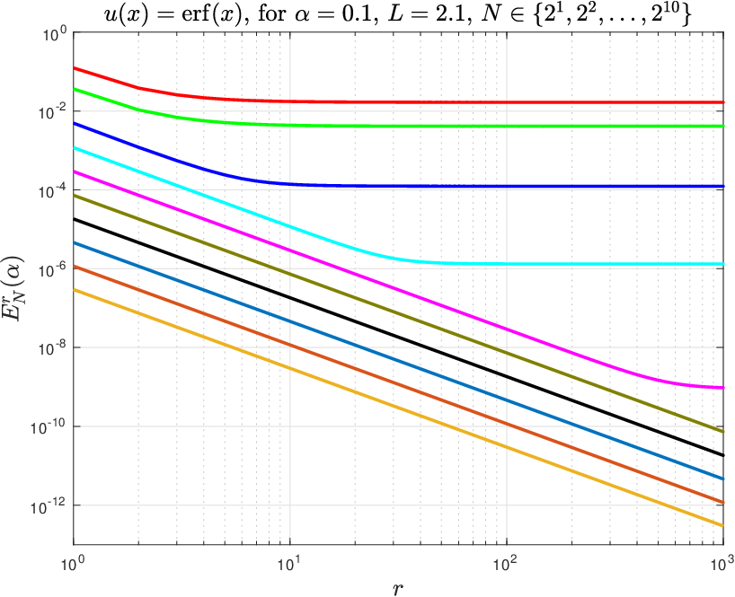
Refer to caption
Refer to caption
Refer to caption
Figure 3: Norms of the errors ENr​(α)E_{N}^{r}(\alpha), as given by (64), for rr and NN, using (57) (left) and (63) (right).

In Figure 3, the curves corresponding to N=210N=2^{10} are below the other curves and, in general, for a fixed rr, the norms of the errors become smaller as NN increases. Therefore, although we have proved theoretically and confirmed numerically the second order of convergence with respect to rr, a natural question that arises is what order of convergence we have if we fix rr and increase NN. Hence, in Figure 4, in order to estimate the order of convergence, we have plotted log2⁡(E2​Nr​(α)/ENr​(α))\log_{2}(E_{2N}^{r}(\alpha)/E_{N}^{r}(\alpha)), for r=1r=1, N∈{21,22,…,210}N\in\{2^{1},2^{2},\ldots,2^{10}\}, and α∈{0.01,…​0.99}∪{1.01,…,1.99}\alpha\in\{0.01,\ldots 0.99\}\cup\{1.01,\ldots,1.99\}; and in Figure 5, the corresponding values of ENr​(α)E_{N}^{r}(\alpha). Although further research is needed here, the results would seem to suggest that ENr​(α)=𝒪⁡(1/N2)E_{N}^{r}(\alpha)=\mathcal{O}(1/N^{2}), i.e., there is also second order of convergence with respect to NN when α∈[0.5,2)\alpha\in[0.5,2), whereas, when α∈(0,0.5]\alpha\in(0,0.5], ENr​(α)=𝒪⁡(1/N1.5+α)E_{N}^{r}(\alpha)=\mathcal{O}(1/N^{1.5+\alpha}).

Refer to caption
Refer to caption
Refer to caption
Figure 4: Numerical measure of the order of convergence of the method. ENr​(α)E_{N}^{r}(\alpha) is given by (64), using (57) (left) and (63) (right).
Refer to caption
Refer to caption
Refer to caption
Figure 5: Norms of the errors of the numerical experiments in Figure 4. ENr​(α)E_{N}^{r}(\alpha) is given by (64), using (57) (left) and (63) (right).

It is a well known fact that some types of differentiation matrices (like Chebyshev differentiation matrices, see, e.g., gottlieb) are severely ill-conditioned. Indeed, the condition numbers of the Chebyshev differentiation matrices of order NN approximating the first and second derivatives behave respectively as 𝒪⁡(N2)\mathcal{O}(N^{2}) and 𝒪⁡(N4)\mathcal{O}(N^{4}). Therefore, it is natural to ask ourselves how our numerical method behaves when 2​N​r2Nr, which is the number of internal nodes, is extremely large. On the left-hand side of Figure 6, we have plotted the discrete L∞L^{\infty} norm of the errors, i.e., ‖(−Δ)α/2​u−(−Δ)numα/2​u‖∞\|(-\Delta)^{\alpha/2}u-(-\Delta)_{\rm num}^{\alpha/2}u\|_{\infty}, for N=10000019N=10000019 (a prime number) and r=1r=1, taking α∈{0.01,…​0.99}∪{1.01,…,1.99}\alpha\in\{0.01,\ldots 0.99\}\cup\{1.01,\ldots,1.99\}. Even if the accuracy greatly depends on α\alpha, it is at least of the order of 𝒪⁡(10−10)\mathcal{O}(10^{-10}) for most values of α\alpha, and still of the order of 𝒪⁡(10−9)\mathcal{O}(10^{-9}) in the worst cases (i.e., when α\alpha is close to both 00 and 22). Besides, it is particularly remarkable that the errors are of the order of 𝒪⁡(10−14)\mathcal{O}(10^{-14}), for a non negligible amount of values of α\alpha, which confirms again that the implementation of the method is correct. On the other hand, in the right-hand side of Figure 6, we have plotted the discrete L∞L^{\infty} norm of the errors, for N=128N=128, and r=216=65536r=2^{16}=65536, and similar conclusions can be drawn, except that the worst results happen only when α\alpha is close to 22. In our opinion, this point is the main caveat of the method and requires further research. However, to the best of our knowledge, as of now, there seems to be no other numerical method capable of approximating the fractional Laplacian at such large amounts of nodes NN (and let alone doing it in just a few seconds), so, even in the worst cases, we think that the accuracy is still remarkably high.

Refer to caption
Refer to caption
Figure 6: Discrete L∞L^{\infty} norms of the errors of the numerical experiments, for very large amounts 2​N​r2Nr of internal points.

6.1 An evolution example

In order to show that the method in this paper can be used to simulate relevant fractional differential equations, we have applied it to the focusing fractional cubic nonlinear Schrödinger equation considered in cayamacuestadelahoz2020 (see the references on this equation in that paper):

{i​∂ψ∂t=12​(−Δ)α/2​ψ−|ψ|2​ψ,t>0,ψ⁡(x,0)=ψ0​(x).\left\{\begin{aligned} &i\frac{\partial\psi}{\partial t}=\dfrac{1}{2}(-\Delta)^{\alpha/2}\psi-|\psi|^{2}\psi,&&t>0,\\ &\psi(x,0)=\psi_{0}(x).\end{aligned}\right. (66)

As in cayamacuestadelahoz2020, we have considered α=1.99>1\alpha=1.99>1, for which (66) has global existence GuoHuo2013; GuoSireWangZhao2018, and have taken ψ0​(x)=exp⁡(−x2)\psi_{0}(x)=\exp(-x^{2}) as the initial data. We use the classical fourth-order Runge-Kutta method to advance in time, and compute the energy M⁡(t)M(t), which is a preserved quantity, to measure the accuracy of the numerical results:

M⁡(t)=∫−∞∞|ψ⁡(x,t)|2​𝑑x=L​∫0π|ψ⁡(L​cot⁡(s),t)|2sin2⁡(s)​𝑑s≈L​πN​∑j=0N−1|ψ⁡(L​cot⁡(sj),t)|2sin2⁡(sj),M(t)=\int_{-\infty}^{\infty}|\psi(x,t)|^{2}dx=L\int_{0}^{\pi}\frac{|\psi(L\cot(s),t)|^{2}}{\sin^{2}(s)}ds\approx\frac{L\pi}{N}\sum_{j=0}^{N-1}\frac{|\psi(L\cot(s_{j}),t)|^{2}}{\sin^{2}(s_{j})},

where, in order to approximate M⁡(t)M(t), we have applied the composite midpoint rule to ψ⁡(L​cot⁡(s),t)/sin2⁡(s)\psi(L\cot(s),t)/\sin^{2}(s) over s∈[0,π]s\in[0,\pi]. This approximation yields spectral accuracy, due to the fact that ψ⁡(L​cot⁡(s),t)/sin2⁡(s)\psi(L\cot(s),t)/\sin^{2}(s) is a regular, periodic function over s∈[0,π]s\in[0,\pi]. The values of the other parameters are N=4096N=4096, L=200L=200, Δ​t=0.01\Delta t=0.01, r∈{20,21,…,26}r\in\{2^{0},2^{1},\ldots,2^{6}\}. On the upper left-hand side of Figure 7, we have plotted in semilogarithmic scale |M⁡(t)−M⁡(0)|=|M⁡(t)−π/2||M(t)-M(0)|=|M(t)-\sqrt{\pi/2}|; the results are coherent with the fact that the approximation of the fractional Laplacian behaves as 𝒪⁡(1/r2)\mathcal{O}(1/r^{2}). Indeed, when we multiply rr by 22, |M⁡(t)−π/2||M(t)-\sqrt{\pi/2}| is approximately divided by 44, which results in the curves corresponding to the different rr being roughly parallel. On the other hand, on the upper right-hand side, we plot the modulus of ψ⁡(x,t)\psi(x,t); on the lower left-hand side, the real part of ψ⁡(x,t)\psi(x,t); and on the lower right-hand side, the imaginary part of ψ⁡(x,t)\psi(x,t); in the three cases, we only show the parts corresponding to x∈[−150,150]x\in[-150,150].

Refer to caption
Refer to caption
Refer to caption
Refer to caption
Figure 7: Upper-left: error in the preservation of the energy E⁡(t)E(t). Upper-right: modulus of ψ⁡(x,t)\psi(x,t). Lower-left: real part of ψ⁡(x,t)\psi(x,t). Lower-right: imaginary part of ψ⁡(x,t)\psi(x,t).

The numerical simulations reveal that the method is very stable for large values of NN and not too small values of Δ​t\Delta t, and the choice of rr allows to a establish a compromise between execution speed and accuracy. Indeed, given an evolution problem involving the fractional Laplacian, it is possible to consider a first, fast executing simulation with r=1r=1, to get an idea of the evolution, and then increase rr. For instance, in the experiments in Figure 7, when r=26=64r=2^{6}=64, the maximum error in the preservation of the energy is equal to 1.1281×10−71.1281\times 10^{-7}, and happens at t=100t=100.

Data Availability Statement

The authors confirm that the data supporting the findings of this study are available within the article.

Declarations

The authors have no competing interests to declare that are relevant to the content of this article.

References

  • (1) Acosta, G., Borthagaray, J.P., Bruno, O., Maas, M.: Regularity theory and high order numerical methods for the (1D)-fractional Laplacian. Math. Comp. 87, 1821–1857 (2018)
  • (2) Bonforte, M., Vázquez, J.L.: Fractional nonlinear degenerate diffusion equations on bounded domains part I. Existence, uniqueness and upper bounds. Nonlinear Analysis 131, 363–398 (2016)
  • (3) Boyd, J.P.: The Optimization of Convergence for Chebyshev Polynomial Methods in an Unbounded Domain. J. Comput. Phys. 45(1), 43–79 (1982)
  • (4) Boyd, J.P.: Spectral Methods Using Rational Basic Functions on an Infinite Interval. J. Comput. Phys. 69(1), 112–142 (1987)
  • (5) Caffarelli, L., Silvestre, L.: An extension problem related to the fractional Laplacian. Commun. Part. Differ. Equ. 32(8), 1245–1260 (2007)
  • (6) Cayama, J., Cuesta, C.M., de la Hoz, F.: Numerical approximation of the fractional Laplacian on ℝ\mathbb{R} using orthogonal families. Applied Numerical Mathematics 158, 164–193 (2020)
  • (7) Cayama, J., Cuesta, C.M., de la Hoz, F.: A pseudospectral method for the one-dimensional fractional Laplacian on ℝ\mathbb{R}. Applied Mathematics and Computation 389(1), 125577 (2021)
  • (8) Chen, S., Shen, J.: An Efficient and Accurate Numerical Method for the Spectral Fractional Laplacian Equation. J. Sci. Comput. (2020)
  • (9) D’Elia, M., Du, Q., Glusa, C., Gunzburger, M., Tian, X., Zhou, Z.: Numerical methods for nonlocal and fractional models. Acta Numer. 29, 1–124 (2020)
  • (10) Duo, S., van Wyk, H., Zhang, Y.: A novel and accurate finite difference method for the fractional Laplacian and the fractional poisson problem. J. Comput. Phys. 355, 233–252 (2018)
  • (11) Duo, S., Zhang, Y.: Accurate numerical methods for two and three dimensional integral fractional Laplacian with applications. Comput. Methods Appl. Mech. Engrg. 355, 639–662 (2019)
  • (12) Frigo, M., Johnson, S.G.: The Design and Implementation of FFTW3. Proceedings of the IEEE 93(2), 216–231 (2005)
  • (13) Gao, T., Duan, J., Li, X., Song, R.: Mean exit time and escape probability for dynamical systems driven by Lévy noises. SIAM J. Sci. Comput. 36, A887–A906 (2014)
  • (14) García-Cervera, C.J.: An Efficient Real Space Method for Orbital-Free Density-Functional Theory. Commun. Comput. Phys. 2(2), 334–357 (2007)
  • (15) Gottlieb, D., Orszag, S.A.: Numerical Analysis of Spectral Methods: Theory and Applications. SIAM (1977)
  • (16) Guo, B., Huo, Z.: Well-posedness for the nonlinear fractional Schrödinger equation and inviscid limit behavior of solution for the fractional Ginzburg-Landau equation. Fractional Calculus and Applied Analysis 16(1), 226–242 (2013)
  • (17) Guo, Z., Sire, Y., Wang, Y., Zhao, L.: On the energy-critical fractional Schrödinger equation in the radial case. Dynamics of Partial Differential Equations 15(4), 265–282 (2018)
  • (18) de la Hoz, F., Cuesta, C.M.: A pseudo-spectral method for a non-local KdV-Burgers equation posed on ℝ\mathbb{R}. J. Comput. Phys. 311, 45–61 (2016)
  • (19) Hu, Y., Li, C., Li, H.: The finite difference method for Caputo-type parabolic equation with fractional Laplacian: One-dimension case. Chaos, Solitons & Fractals 102, 319–326 (2017)
  • (20) Huang, Y., Oberman, A.: Numerical methods for the fractional Laplacian: A finite difference-quadrature approach. SIAM J. Numer. Anal. 52, 3056–3084 (2014)
  • (21) Huang, Y., Oberman, A.: Finite difference methods for fractional Laplacians. arXiv:1611.00164 (2016)
  • (22) Kapur, S., Rokhlin, V.: High-Order Corrected Trapezoidal Quadrature Rules for Singular Functions. SIAM Journal on Numerical Analysis 34(4), 1331–1356 (1997). DOI 10.1137/S0036142995287847. URL http://epubs.siam.org/doi/10.1137/S0036142995287847
  • (23) Krasny, R.: A study of singularity formation in a vortex sheet by the point-vortex approximation. J. Fluid. Mech. 167, 65–93 (1986)
  • (24) Kwaśnicki, M.: Ten equivalent definitions of the Fractional Laplace Operator. Fract. Calc. Appl. Anal. 20(1), 7–51 (2017)
  • (25) Lyness, J.N., Ninham, B.W.: Numerical Quadrature and Asymptotic Expansions. Mathematics of Computation 21(98), 162–178 (1967)
  • (26) Mao, Z., Karniadakis, G.: A spectral method (of exponential convergence) for singular solutions of the diffusion equation with general two-sided fractional derivative. SIAM J. Numer. Anal. 56, 24–29 (2018)
  • (27) Minden, V., Ying, L.: A simple solver for the fractional laplacian in multiple dimensions. SIAM Journal on Scientific Computing 42(2), A878–A900 (2020)
  • (28) Navot, I.: An extension of the Euler-Maclaurin summation formula to functions with a branch singularity. J. Math. and Phys. 40, 271–276 (1961)
  • (29) Nochetto, R., Otárola, E., Salgado, A.: A PDE approach to fractional diffusion in general domains: a priori error analysis. Found. Comput. Math. 15(3), 733–791 (2015)
  • (30) Quarteroni, A., Sacco, R., Saleri, F.: Numerical Mathematics, (2nd edition) edn. Springer (2007)
  • (31) Sheng, C., Shen, J., Tang, T., Wang, L.L., Yuan, H.: Fast Fourier-like Mapped Chebyshev Spectral-Galerkin Methods for PDEs with Integral Fractional Laplacian in Unbounded Domains. SIAM Journal on Numerical Analysis 58(5), 2435–2464 (2020)
  • (32) The MathWorks Inc.: MATLAB, Version R2022a (2022). URL https://www.mathworks.com
  • (33) Tian, X., Du, Q.: Analysis and comparison of different approximations to nonlocal diffusion and linear peridynamic equations. SIAM J. Numer. Anal. 51, 3458–3482 (2013)
  • (34) Waterman, P.C., Yos, J.M., Abodeely, R.J.: Numerical integration of non-analytic functions. J. Math. and Phys. 43, 45–50 (1964)
  • (35) Weideman, J.A.C.: Computing the Hilbert transform on the real line. Mathematics of Computation 64(210), 745–762 (1995)
  • (36) Wolfram Research, Inc.: Mathematica, Version 13.0 (2022). URL https://www.wolfram.com
  • (37) Zayernouri, M., Karniadakis, G.: Fractional spectral collocation method. SIAM J. Sci. Comput. 36, A40–A62 (2014)