All-in-One: A Highly Representative DNN Pruning Framework for Edge Devices with Dynamic Power ManagementConference: IEEE/ACM International Conference on Computer-Aided Design; ; San Diego, CA, USAIEEE/ACM International Conference on Computer-Aided Design (ICCAD ’22), October 30-November 3, 2022, San Diego, CA, USAPrice: 15.00DOI: 10.1145/3508352.3549379ISBN: 978-1-4503-9217-4/22/10
Abstract.
During the deployment of deep neural networks (DNNs) on edge devices, many research efforts are devoted to the limited hardware resource. However, little attention is paid to the influence of dynamic power management. As edge devices typically only have a budget of energy with batteries (rather than almost unlimited energy support on servers or workstations), their dynamic power management often changes the execution frequency as in the widely-used dynamic voltage and frequency scaling (DVFS) technique. This leads to highly unstable inference speed performance, especially for computation-intensive DNN models, which can harm user experience and waste hardware resources. We firstly identify this problem and then propose All-in-One, a highly representative pruning framework to work with dynamic power management using DVFS. The framework can use only one set of model weights and soft masks (together with other auxiliary parameters of negligible storage) to represent multiple models of various pruning ratios. By re-configuring the model to the corresponding pruning ratio for a specific execution frequency (and voltage), we are able to achieve stable inference speed, i.e., keeping the difference in speed performance under various execution frequencies as small as possible. Our experiments demonstrate that our method not only achieves high accuracy for multiple models of different pruning ratios, but also reduces their variance of inference latency for various frequencies, with minimal memory consumption of only one model and one soft mask.
1. Introduction
As deep neural networks (DNNs) can achieve superior performance compared with traditional methods, they have been applied to a wide range of applications including classification (He et al. 2016), object detection (Bochkovskiy et al. 2020), natural language processing (Vaswani et al. 2017), and so on recently. Besides, due to the rapid increasing popularity of edge devices such as mobile phones, and tablets, there are ever-increasing demands for deploying DNNs on various resource-limited edge devices.
When deploying DNNs from powerful servers (or workstations) to resource-intensive edge devices, we need to deal with the significant difference of (i) hardware resource and (ii) energy support. The hardware resource usually refers to the available memory, computation units (such as multiplier–accumulator) and so on. Many works (Wen et al. 2016; Guo et al. 2016; Min et al. 2018; He et al. 2018; Zhang et al. 2018a; Zhang et al. 2018b; Zhang et al. 2021; Jian et al. 2021; Zhan et al. 2021; Wu et al. 2022; Yuan et al. 2021) investigate how to keep or improve the DNN performance under a more rigid resource constraint (such as limited memory or floating point operations per second (FLOPS)).
Though the resource limitation of edge devices receives much attention from researchers, there are little research efforts devoted to the energy support. The energy support refers to the power or energy (including the execution frequency and voltage) to support the execution of DNNs when performing DNN inference on edge devices. Different from servers or workstations with plenty of power support, edge devices only have a budget of energy (such as battery) and need to adopt certain dynamic strategies to manage the energy usage. For example, if the battery level decreases to 15% (or 10%) on a mobile phone, it usually switches to the energy saving mode and reduces the execution frequency to achieve longer availability. Besides energy saving mode, the dynamic voltage and frequency scaling (DVFS) technique is widely adopted on edge devices to adjust the power and speed settings so that the resource allotment for tasks can be optimized and the power saving can be maximized. In general, the current energy support with dynamic frequencies is unstable for the deployment of DNNs on edge devices.
The unstable energy support leads to unstable DNN performance in terms of inference speed or latency. If the execution frequency switches to a smaller value, the computation-intensive DNN models need more time to finish the computations, incurring larger inference latency. The unstable inference latency not only harms the user experience, but also wastes a lot of hardware resources. DNNs with original real-time inference capability can hardly achieve real-time inference when the execution frequency decreases, incurring stuttering or lag, and poor user experience. Besides, for safety-critical applications on real-time embedded systems like medical monitoring on smart watches, the deadline based scheduling is used to guarantee safety. The deadlines are usually set up based on the worst-case execution time, which could waste many processor resources if the worst-case execution time with low execution frequency is much larger than normal values.
To improve user experience and save hardware resource, it is necessary to make the DNN performance (especially speed performance) as stable as possible under different levels of energy support (especially the execution frequency). Different from the hardware resource limitation which many research efforts focus on during DNN deployment, little attention is paid to the unstable energy support or dynamic frequency management. Our work firstly identify the unstable energy and frequency problem during DNN deployment and propose a framework to deal with the limited hardware resource and unstable energy support. To deal with various execution frequencies, our framework can generate multiple sparse models with different sparsity ratios, such that higher-sparsity models with less computations can run with a smaller frequency, leading to smaller variance of the inference time. To achieve this, we propose parametric pruning together with switchable thresholds and batch normalization. Thus, after training one model and one soft mask, we can use switchable thresholds to convert the soft mask into different binary hard masks of various sparsity ratios to deal with different execution frequencies. Besides, we further adopt switchable batch normalization to improve the accuracy performance of each sparse model. Our memory cost is only one highly representative single model and a soft mask, which is much lower than the cost of training and storing multiple sparse models separately. As a result, our work can deal with the limited hardware resource and unstable energy support on edge devices simultaneously. We summarize our contributions as follows.
- •
We firstly identify the unstable energy support problem with dynamic frequencies for DNN deployment on edge devices and evaluate the influence of dynamic frequency and power for DNN inference.
- •
To deal with the limited hardware resource and unstable energy support on edge devices, we propose parametric pruning together with switchable threshold and batch normalization to generate one single highly representative model and soft mask, which can represent multiple sparse models to work with different execution frequency.
- •
Our experimental results demonstrate that we can use a minimal memory cost with one model and one rescaled soft mask, to obtain multiple models of various sparsity levels with state-of-the-art classification accuracy compared with baseline methods. Moreover, by using a higher-sparsity model for a lower frequency, we can keep the latency under various frequencies as close as possible and significantly reduce the variance of the inference latency.
2. Related work
2.1. Sparse Models
Weight pruning (Wen et al. 2016; Guo et al. 2016; Min et al. 2018; He et al. 2018; He et al. 2019) is an effective method to reduce model redundancy. Various pruning methods with different sparsity types have been proposed in the literature. Irregular pruning (Han et al. 2015) achieves high accuracy but the reduction in parameters cannot be transformed into inference speedup. Structured sparsity (Min et al. 2018; Zhuang et al. 2018; Zhu et al. 2018; Ma et al. 2020c; Zhao et al. 2019; Liu et al. 2020) such as column pruning and row pruning are hardware-friendly, but the coarse-grained pruning nature causes accuracy degradation. Recently proposed fine-grained structured pruning regularities including pattern-based pruning (Ma et al. 2020a; Niu et al. 2020; Gong et al. 2020) and block-based pruning (Dong et al. 2020; Li et al. 2020; Ma et al. 2020b; Gong et al. 2021) preserve high accuracy while maintaining structures that can be exploited by compiler for hardware accelerations. However, most of the sparse model methods focus on the fixed resource scenarios without considering the hardware environment change. The resulting models have one fixed architecture and parameters that only satisfy one sparsity ratio.
2.2. Re-configurable DNNs
To obtain multiple models with different sparsity ratios, the most straightforward method is to train multiple models with different sizes using the sparse model methods. However, this causes huge computation burden during training and requires storing multiple models on the device. To decrease the computation and storage cost, recent works consider to train efficient architectures that can be re-configured at runtime. NS (Yu et al. 2018) and US-Nets (Yu and Huang 2019) train a model with multiple switches corresponding to different number of channels. This method simply retains the channels in the front of each layer, which neglects the different importance of each channel to the whole model performance. Furthermore, removing entire channels incurs severe accuracy loss. Joslim (Chin et al. 2021) extends in this direction by further allowing the joint optimization of width configurations and weights. But the method still relies on the coarse-grained structure pruning, incurring accuracy loss. Paper (Cai et al. 2019) proposes to train a large dense model and queries sub-models upon requirement. However, the method has to store a dense model and needs additional weights to achieve model transformation. LCS (Nunez et al. 2021) learns a compressible subspace to obtain models with different sparsity ratio settings, but the accuracy degradation is non-negligible. RT3 (Song et al. 2021) discovers multiple pattern sets with different sparsity ratio settings to be switched during runtime. The drawback is that the pattern sets have to be stored individually, consuming a large amount of storage, and are too irregular to achieve efficient hardware accelerations.
3. Motivation
| N1 | N2 | N3 | N4 | N5 | |
| clk/freq (mHz) | 305 | 400 | 442 | 525 | 587 |
| Vol (mV) | 0.47-0.73 | 0.52-0.79 | 0.55-0.84 | 0.58-0.89 | 0.61-0.90 |
Many deep learning (DL) based applications are deployed on edge devices such as mobile phones. Although many research efforts are devoted to the limited hardware resource on edge devices, little attention is paid to the influence of unstable energy support or dynamic frequency management. As edge devices typically only have a budget of energy with batteries (rather than almost unlimited energy support on servers or workstations), their dynamic power management often changes the execution frequency, leading to highly unstable inference speed performance, especially for computation-intensive DNN models. Table 1 demonstrates the available Frequency/Voltage levels on Adreno 650 GPU in OnePlus T8 platform. For example, if the battery level of a OnePlus T8 phone is below 15%, the phone switches to the energy saving mode and the frequency is reduced to 52% of that of full battery. The significant reduction on the frequency leads to longer inference time for these computation-intensive DL applications. We observe that the dense ResNet-18 on ImageNet dataset takes 18.86 ms to inference on the mobile GPU. But after the mobile frequency reduces to 52%, the inference time extends to 30.74 ms, 62.99% longer. Besides the energy saving mode, the DVFS technique is widely applied on edge devices to adjust the power and frequency to optimize resource allotment for tasks and maximize power saving. It is common that the applications need to run under dynamic execution frequencies.
If the frequency becomes smaller, the model may be slower with longer inference time. The DNNs with original real-time inference capability may fail to achieve real-time inference and cause stuttering or lag, leading to poor user experience. Besides user experience, many hardware resource can be wasted. For example, for safety-critical applications like medical monitoring on smart watches, the deadline based scheduling is used by the real-time scheduler to guarantee safety. The deadlines are usually set up based on the worst-case execution time, which could waste many processor resources if it is much larger than normal values.
To guarantee user experience and save hardware resource, we should keep consistent performance of DL applications (especially speed performance), under various execution frequencies. In this paper, we focus on image classification application as an example. But our method is not only limited to image classification. To keep consistent speed performance under different frequencies, inspired by the model pruning methods to achieve on-mobile real-time inference, we propose to use one model with switchable different pruning masks corresponding to various sparsity ratios. Thus, for higher frequency where the computation could be faster, we can adopt the mask with fewer pruned weights and more computations. For lower frequency where the computation could be slower, we can switch to the mask with more pruned weights and fewer computations. In this way, we may keep the inference latency under different execution frequency as close as possible.
We highlight that it is non-trivial to design such one model with multiple switchable pruning masks corresponding to various sparsity ratios. One naive alternative method is to train multiple pruned models, each model corresponding to one single sparsity ratio. However, DL models usually consume a lot of memory and the available memory on mobile devices is limited. Thus, we choose the method with one single model and multiple masks for this model. There are still several requirements for this method: (i) The memory cost of each mask should be significantly smaller than the whole model to save memory cost. (ii) The accuracy under each mask should be as high as possible. We should keep consistent classification performance after switching to different masks.
Our setting is different from previous pruning work (Wen et al. 2016; Guo et al. 2016; Min et al. 2018; He et al. 2018; He et al. 2019) as most pruning methods only design one single pruning mask for one model given one sparsity ratio. Specifically, our work designs multiple pruning masks simultaneously for one model and each mask can achieve high classification accuracy under the corresponding sparsity ratio. Compared with methods with only a single mask design, our work has the following advantages: (i) The training cost is saved. After the training, we can obtain multiple sparse masks corresponding to multiple sparsity ratios simultaneously, while the single mask design methods need to run their algorithm multiple times to obtain multiple masks, incurring much larger training cost. (ii) The memory cost is saved. The single mask design methods usually need to fine-tune based on each mask to improve the final accuracy. Thus, each mask is not able to represent the pruned model and each pruned model is stored instead of each mask, incurring much larger memory cost. Moreover, we further adopt switchable threshold and batch normalization to derive one highly representative model and one soft mask so that multiple sparse models can be obtained from them. Thus the memory cost can be further saved.
4. Proposed Method
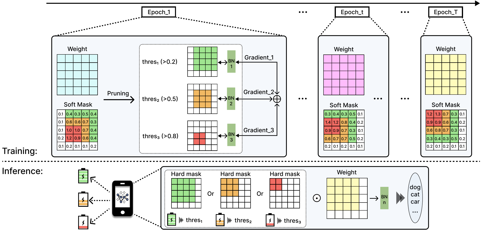
The framework overview of All-in-One in the case of three battery modes is illustrated in Figure 1. Our objective is to design one model and multiple masks where each mask corresponds to one sparsity ratio under a certain battery mode. The model can be easily switched during inference. When the frequency becomes smaller (battery level is lower), the model can switch to a mask with a larger sparsity ratio and becomes more sparse with fewer computations. Thus though the computation may be slower with lower frequency, the inference time with the more sparse model may not change greatly. More specifically, as in the Figure 1, a sparse model with green mask is used when the battery level is high. When the battery level decreases, the framework switches to use the orange mask. As the battery is almost out of power, the mask is switched to the red one. The switch can be achieved instantly without any retraining.
To achieve this, we propose the parametric pruning method to parameterize the pruning. The traditional pruning usually needs the in-differentiable sorting operations, which are unfriendly for the model training especially with multiple sparse masks. With the proposed parametric pruning, we do not need to incorporate sorting operations, improving pruning and training efficiency. As different sparsity ratios cause different mean and variance for the feature map, we further adopt switchable batch normalization (BN) to improve the classification accuracy under each sparsity ratio.
Based on the parametric pruning, we use switchable threshold to switch among masks of various sparsity ratios during training. When deployed for inference, the soft mask and switchable thresholds can be further re-scaled into low-bit format. Therefore, we do not need to store binary masks for sparsity ratios. Instead, we only need to store one re-scaled mask together with multiple thresholds (each threshold can determine one binary mask based on the re-scaled mask). The re-scaled threshold transforms the re-scaled soft mask into the corresponding hard mask when the battery mode changes. The hard mask with a higher threshold value is the subset of the hard mask with a lower threshold value. For instance, in Figure 1, the mask in red color which corresponds to the low battery mode is the subset of the mask in green color. Furthermore, instead of storing the entire dense model on the mobile device, only the weights in the largest compact model needs to be stored, which significantly reduces the memory cost. Taking Figure 1 as an example, there is no need to store the entire 55 weight matrix. Alternatively, the 44 weight matrix is stored. Detailed designs are presented in the following sections.
4.1. Pruning Schemes
In this work, we adopt fine-grained structured pruning including pattern-based pruning and block-based pruning, to efficiently accelerate the on-mobile inference while maintaining high accuracy. For both of the pruning schemes, the only set of weights to be stored is the largest compact model to accommodate the limited storage resources on the edge devices.
Pattern-based pruning. Pattern-based pruning is a combination of kernel pattern pruning and connectivity pruning, as shown in Figure 2 (a), where grey color represents removed weight. Kernel pattern pruning removes a fixed number of weights in each kernel and the locations of the remaining weights form specific patterns. The total number of pattern styles in the pattern library is limited for hardware accelerations. In our framework, each kernel pattern reserves 4 non-zero weights to match the single-instruction multiple-data (SIMD) architecture of embedded CPU/GPU processors to maximize the hardware throughput. As the sparsity ratio is constant for kernel pattern pruning, connectivity pruning is adopted as the supplementary to kernel pattern pruning for a higher sparsity ratio. Connectivity pruning cuts the connections between certain input and output channels, which is equivalent as removing whole kernels. To provide a re-configurable sparse model with switches, our framework first applies kernel pattern pruning to obtain a compressed model. different levels of connectivity pruning are further applied to the kernel pattern pruned model so that models of different sparsity are available at runtime.
Block-based pruning. Block-based pruning divides the weight matrix into equal-sized blocks and apply independent column pruning for each block, as shown in Figure 2 (b). To find a re-configurable sparse model, our framework prunes columns in each block with different sparsity ratio settings to obtain well-trained switches.
4.2. Parametric Pruning
We first need to make the pruning parametric to avoid the use of in-differentiable sorting operations. To achieve this, we assign importance scores to groups of weights. Let denote the weights for the -th convolution (CONV) layer, with output channels, input channels, and kernels of size . The output feature of the -th layer is represented as , with channels and feature size. The operation for the -th layer is represented as , where denotes the convolution operation. For pattern-based pruning, as kernel pattern pruning results in a fixed sparsity ratio, a higher sparsity is achieved by pairing with connectivity pruning that removes whole kernels. Therefore, to perform connectivity pruning, for each kernel , in the -th layer, we assign an importance score as a soft mask to weight the importance of each kernel. The importance scores in the -th layer form the soft mask matrix . For block-based pruning, the weight matrix is first reshaped to a 2D matrix with size and divided into equal-sized blocks with size , namely, . An importance score is assigned for each column in every block .
We use each element of as the pruning indicator for corresponding weights. Larger value of indicates a more important group of weights that should be preserved while smaller value means that the weights may be removed. In this problem, we would like to achieve level sparsity, i.e., target sparsity ratios. The -th target sparsity ratio is paired with a predefined threshold value to convert the score into a binary mask as below,
| (1) |
where is the binarized . The non-binary is a soft mask and the binary is a hard mask. During the inference of model pruning and training, we first obtain the binary mask from . Then we apply the binary mask to the corresponding weights following in each layer to achieve kernel or block pruning. means that the group of weights is reserved and means the group of weights is pruned.
Thus we are able to obtain a binary mask for weights in each CONV layer. The next problem is how to make the soft mask trainable, as the binarization operation is non-differentiable, leading to difficulties for back-propagation. To solve this, we integrate Straight Through Estimator (STE) (Bengio et al. 2013) as shown below,
| (2) |
where we can directly pass the gradients through the binarization. STE is originally applied in quantization tasks (Liu and Mattina 2019; Yin et al. 2019) to avoid the non-differentiable issues. If we do not use STE, more complicated strategies may be applied to deal with non-differentiable binary masks such as (Guo et al. 2020; Guan et al. 2020). With binarization and STE, we are able to build a trainable soft mask to incorporate pruning in model training without using sorting operations. The trainable mask has the following advantages: (i) The soft mask can be efficiently trained along with the network parameters via gradient descent optimizers, thus saving training cost compared with (Guo et al. 2020; Guan et al. 2020). (ii) Different from previous methods (Han et al. 2015; Yu et al. 2017; He et al. 2017), which determine the pruning according to the parameter magnitudes, we use the soft mask to serve as the pruning indicator, rather than the parameter magnitudes. Thus pruning is decoupled from the parameter magnitudes.
We can train the model weights and the soft masks simultaneously. As we need to achieve high accuracy for multiple sparsity ratios, one model and one soft mask is not able to achieve this. So we assign each sparsity ratio a corresponding threshold and batch normalization parameters as introduced in Sec. 4.3 and Sec. 4.4, respectively. The classification loss can be expressed as , where denotes the model weights, represents the soft mask, and denote the threshold and the BN parameters for the -th sparsity ratio, respectively. Note that and are shared between different sparsity ratios when performing training and inference. Besides and , each sparsity ratio has its specific threshold and BN parameters.
4.3. Switchable Threshold
Given level sparsity or sparsity ratios, we can design masks where each mask can satisfy one sparsity ratio. However, multiple masks still cost a lot of memory. To further reduce the memory cost, based on the parametric pruning, we can only use one soft mask with thresholds (i.e., scales with negligible memory cost). For each sparsity ratio, we can use the soft mask and the corresponding threshold following Eq. (1) to obtain the binary mask for this sparsity ratio. The illustration of the switchable threshold is shown in Figure. 3. By using a higher threshold value, more weights are removed, which are denoted with the light blue circles. With the switchable threshold, the more sparse model uses a subset of the collection of weights in a more dense model.
4.4. Switchable Batch Normalization
As accumulating model parameters with different sparsity ratio results in different feature mean and variance, the discrepancy across different configurations leads to inaccurate statistics of shared BN layers. Therefore, to maintain high accuracy for each sparsity ratio, we create independent BN parameters for each sparsity ratio, as shown in Figure 4. When inference under the sparsity ratio , only the corresponding BN with parameters participates into the computation. With the switchable BN, for a model with target sparsity ratios, we need to store set of BN parameters. In most cases, BN layers only have less than 1% of the model size. Besides, the BN runtime cost is also negligible for deployment. Compared to separately trained models or using two sets of weights for learning compressible subspaces (Nunez et al. 2021), the usage of switchable BN is memory efficient while keeping competitive accuracy performance.
4.5. Training Method
With the differentiable soft mask, we can train and prune the model via SGD simultaneously with the loss function,
| (3) |
where is the cross entropy classification loss, and is the regularization term related to the computation complexity. For simplicity, we take Multiply-Accumulate operations (MACs) as the constraint/target rather than parameter number to estimate on-device execution cost. can weight the loss and stabilize training. can be simply defined as norm between current MACs and target MACs . For connectivity pruning, is defined as
| (4) |
where is obtained by converting the score into binary values according to Eq. (1), and indicates the number of remaining kernels in the -th layer. The constant 4/9 is attributed to kernel pattern pruning that reserves four weights in each kernel.
For block-based column pruning, is defined as
| (5) |
where represents the number of the remaining columns in the block of the -th layer.
Given different battery modes, we could set different target MACs to satisfy different sparsity ratio requirements and form a list of target MACs as . With parametric pruning and switchable threshold & BN, we can perform our training following Algorithm 1. With target MACs, in every iteration, for each target MACs, we first switch to the corresponding and BN parameters, and then compute the loss with the target MACs to obtain gradients through back-propagation. After we collect and accumulate the gradients of all target MACs, we update the weights. Note that the model weights and the soft masks are updated with the gradients accumulated through all target MACs since they are shared between various target MACs. But the BN parameters are updated with the gradients of the single corresponding target MAC, rather than the accumulated gradients, as the BN parameters are switched when moving to another target sparsity ratio.
4.6. Cost Analysis
To satisfy the a total of sparsity ratios simultaneously, we only need to store one model, one re-scaled soft mask, re-scaled thresholds, and sets of BN, where the memory cost of thresholds and BN are negligible. With a well-trained soft mask, there is no need to store its precise floating point values during inference. To save the storage cost, the soft mask can be transformed/re-scaled into the low-bit format (named the re-scaled soft mask). For instance, for , the re-scaled soft mask is composed of values of 0, 1, and 2, with element 2 indicating the scores for the most compact model corresponding to the lowest frequency. Besides, since we perform kernel or block pruning and the soft mask corresponds to the number of kernels or columns/rows in the block rather than all parameters in the model, the memory cost of the soft mask is much smaller than the model weights. Our method can greatly reduce the memory cost compared with using models for sparsity ratios.
5. Experiment results
In this section, we compare All-in-One with state-of-the-art re-configurable DNN methods. The comparison is conducted on both CIFAR-10 and ImageNet datasets. We demonstrate the following: (i) By comparing All-in-One with baseline methods, All-in-One can maintain high accuracy under different sparsity ratio settings with only one set of model weights. (ii) Through real implementations on an off-the-shelf mobile device, All-in-One can mitigate the problem of unstable inference time due to the change of battery level.
5.1. Experiment Setting
In order to evaluate whether All-in-One can consistently attain efficient pruned models for tasks with different complexities, we test on two major image classification datasets, i.e., CIFAR-10 and ImageNet. For CIFAR-10, we experiment with Resnet-18, Resnet-20, and Resnet-32. For ImageNet dataset, we experiment on Resnet-18 and MobileNet-v2. We conduct our multi-model training method on an NVIDIA GTX 1080Ti GPU server using Pytorch. During pruning, The SGD optimizer is utilized with a learning rate of .
All the mobile results are measured on the GPU of an OnePlus 8T mobile phone, which has a Li-Po 4500 mAh battery. The phone itself is equipped with a Qualcomm Snapdragon 865 mobile platform which including a Qualcomm Kryo 585 Octa-core CPU and a Qualcomm Adreno 650 GPU. The same compiler techniques in (Niu et al. 2020) are applied to optimize the DNN execution.
5.2. Accuracy Performance
The accuracy performance on the CIFAR-10 dataset is shown in Table 2. We run our method with pattern-based pruning and block-based pruning respectively and obtain two sets of accuracy. The results show that All-in-One can maintain high accuracy for all switches with only one set of model weights. It significantly outperforms all other state-of-the-art re-configurable DNN methods on all three models with non-negligible improvements (such as our accuracy above 94% v.s. 92% or lower from baseline methods for Resnet-32). Besides, our method with pattern-based pruning usually achieves higher accuracy than ours with block-based pruning.
The accuracy improvements of All-in-One are mainly attributed to two aspects. The first is the fine-grained structured pruning scheme that removes weight at a finer granularity compared to US-Net (Yu and Huang 2019) and LCS-S (Nunez et al. 2021) that employs coarse-grained structured pruning. The second is the separate BN for each configuration that preserves the distinct mean and variance with different sparsity ratios, which is not considered in RT3 (Song et al. 2021).
We further evaluate on the ImageNet dataset and the results are shown in Table 3. For Resnet-18, both pattern-based pruning and block-based pruning are conducted. For MobileNet-v2, as the computations are mainly from 11 CONV layers, which is not suitable for pattern-based pruning, the results using block-based pruning are presented. According to the results, All-in-One again provides the best accuracy performance on both models for each switch in the re-configurable model with non-negligible improvements compared with baseline methods (such as our accuracy above 67% v.s. 65% or below from baselines for the 350M MACs case).
In general, All-in-One possesses the ability to maintain high accuracy for each switch with only one set of weights. When the battery level changes, the model can be easily switched with negligible accuracy degradation compared to other re-configurable DNN methods, greatly improving user experience.
| Method | Pruning Scheme | MACs under Resnet-18 | ||
| 250M | 80M | 40M | ||
| RT3 (Song et al. 2021) | Unstructured | 92.86 | 91.88 | 87.10 |
| All-in-One (Block) | Structured | 94.98 | 94.61 | 94.01 |
| All-in-One (Pattern) | Structured | 95.19 | 94.59 | 93.89 |
| MACs under Resnet-20 | ||||
| 20M | 11M | 7M | ||
| US-Net (Yu and Huang 2019) | Structured | 90.77 | 89.13 | 87.10 |
| Joslim (Chin et al. 2021) | Structured | 90.99 | 89.43 | 87.43 |
| LCS-S (Nunez et al. 2021) | Structured | 86.56 | 83.13 | 78.75 |
| LCS-U (Nunez et al. 2021) | Unstructured | 89.58 | 87.51 | 85.29 |
| RT3 (Song et al. 2021) | Unstructured | 88.13 | 86.62 | 83.83 |
| All-in-One (Block) | Structured | 91.83 | 91.23 | 90.65 |
| All-in-One (Pattern) | Structured | 92.49 | 90.97 | 90.42 |
| MACs under Resnet-32 | ||||
| 33M | 20M | 13M | ||
| US-Net (Yu and Huang 2019) | Structured | 92.06 | 90.56 | 89.83 |
| Joslim (Chin et al. 2021) | Structured | 92.26 | 90.70 | 89.82 |
| RT3 (Song et al. 2021) | Unstructured | 91.04 | 90.03 | 86.31 |
| All-in-One (Block) | Structured | 94.79 | 94.55 | 94.05 |
| All-in-One (Pattern) | Structured | 95.07 | 94.63 | 94.31 |
| Method | Pruning Scheme | MACs under Resnet-18 | ||
| 850M | 480M | 350M | ||
| US-Net (Yu and Huang 2019) | Structured | 66.51 | 63.42 | 61.49 |
| Joslim (Chin et al. 2021) | Structured | 68.49 | 64.51 | 61.82 |
| LCS-S (Nunez et al. 2021) | Structured | 57.61 | 53.70 | 51.30 |
| LCS-U (Nunez et al. 2021) | Unstructured | 68.75 | 67.51 | 65.62 |
| RT3 (Song et al. 2021) | Unstructured | 66.72 | 65.39 | 63.87 |
| All-in-One (Block) | Structured | 69.97 | 68.28 | 67.02 |
| All-in-One (Pattern) | Structured | 70.22 | 69.28 | 67.87 |
| MACs under MobileNet-v2 | ||||
| 210M | 170M | 150M | ||
| US-Net (Yu and Huang 2019) | Structured | 69.71 | 68.19 | 67.59 |
| Joslim (Chin et al. 2021) | Structured | 70.60 | 69.90 | 69.10 |
| RT3 (Song et al. 2021) | Unstructured | 68.12 | 66.97 | 65.65 |
| All-in-One (Block) | Structured | 70.79 | 70.01 | 69.25 |
5.3. Speed Performance
To show that All-in-One can reduce the inference variance when the frequency changes, we show the speed performance comparison of single model and our method. Table 4 and 5 show the results for ImageNet with and under various GPU frequencies on mobile devices using Resnet-18. Single model refers to the case with one single model to work with various frequencies.
| Method | MACs under Resnet-18 | Latency under various GPU frequencies (ms) | Var. of latency | Reduct. rate | |
| 400mHz | 525mHz | ||||
| Dense | 1820M | 33.7 | 28.1 | 15.68 | – |
| Single model (Block) | 480M | 25.7 | 21.6 | 8.41 | 187 |
| Single model (Block) | 350M | 21.9 | 18.6 | 5.45 | 121 |
| All-in-One (Block) | 480M, 350M | 21.9 | 21.6 | 0.045 | 1 |
| Single model (Pattern) | 480M | 25.9 | 22.0 | 7.61 | 381 |
| Single model (Pattern) | 350M | 22.2 | 18.9 | 5.45 | 272 |
| All-in-One (Pattern) | 480M, 350M | 22.2 | 22.0 | 0.02 | 1 |
From Table 4 and 5 we can notice that our structured pruning scheme can achieve inference speedup compared to the dense model on both datasets. Though reducing the latency, using a single sparse model cannot provide stable inference when the frequency changes. Different from single model, our method can dynamically reconfigure to a suitable model once the frequency switches. For example, in the case of , our method can generate three sparse models with different MACs of 850M, 480M, and 350M on ImageNet. The more sparse model is used for the lower frequency. For example, in Table 5, given three frequencies 305mHz, 442mHz, and 587mHz, the model with 850M MACs is applied for the 587mHz frequency, the model with 480M MACs is used for the 442mHz, and the model with 350M MACs is adopted for the 305mHz.
Combining the results in Table 4 and 5, we have the following observations. (i) A more sparse model runs faster under the same frequency (such as 29.1ms for the model with 850M MACs v.s. 23.5ms for the model with 480M MACs under 442mHz using block-based pruning in Table 5). (ii) Besides, for the same model, a higher frequency leads to a faster inference speed (such as 21.9ms under 400mHz v.s. 18.6ms under 525mHz for the model with 480M MACs in Table 4). The significant changes of the inference latency under various frequencies lead to large variance of inference latency (such as 29.64 for the single block-pruned model with 850M MACs in Table 5).
To deal with the different execution frequencies, our method uses models of various sparsity levels so that a more sparse model with less computations can be adopted for a lower frequency, leading to a smaller change to the inference latency. As shown in the results, the latency under difference frequencies are very close with our method (such as 21.9ms and 21.6ms under 400mHz and 525mHz, respectively, in Table 4). All-in-One can significantly reduce the variance of the inference latency. For example, In the case of on ImageNet, our variance with pattern-based pruning is just 0.02, much lower than the single pattern-based sparse model with 480M MACs (7.61) or the sparse model with 350M MACs (5.45), with a reduction rate on the latency variance as high as 381. In the case of , our variance is 0.76 and 0.97 for block-based and pattern-based pruning, respectively, also significantly smaller than the variance of the single model method.
We further show the variance on the CIFAR-10 dataset using Resnet-32 in Figure. 5, where the red line is the worst-case execution time. All-in-One not only reduces the inference time compared to storing a dense model but also mitigates the inference variance problem due to frequency change.
| Method | MACs under Resnet-18 | Latency under various GPU frequencies (ms) | Var. of latency | Reduct. rate | ||
| 305mHz | 442mHz | 587mHz | ||||
| Dense | 1820M | 37.5 | 31.9 | 26.6 | 29.71 | – |
| Single model (Block) | 850M | 35.7 | 29.1 | 24.9 | 29.64 | 39.0 |
| Single model (Block) | 480M | 29.7 | 23.5 | 18.8 | 29.89 | 39.3 |
| Single model (Block) | 350M | 25.1 | 20.3 | 15.8 | 21.63 | 28.5 |
| All-in-One (Block) | 850M, 480M, 350M | 25.1 | 23.5 | 24.9 | 0.76 | 1 |
| Single model (Pattern) | 850M | 35.9 | 29.4 | 25.5 | 27.60 | 28.5 |
| Single model (Pattern) | 480M | 30.1 | 23.7 | 19.0 | 31.04 | 32.0 |
| Single model (Pattern) | 350M | 25.3 | 20.6 | 16.0 | 21.62 | 22.3 |
| All-in-One (Pattern) | 850M, 480M, 350M | 25.3 | 23.7 | 25.5 | 0.97 | 1 |
5.4. Memory Cost
We compare the memory cost of our method and other baselines in Table 6. To obtain models of sparsity ratios, our method only need to store one model and one re-scaled soft mask. Since each element of the mask represents a group of weights, the memory cost of a soft mask is much smaller than that of a model. For other methods, the naive method to train multiple models each for a sparsity ratio needs to store models. RT3 (Song et al. 2021) needs to store a model and masks so that each mask can convert the dense model into a sparse model corresponding to a specific sparsity ratio. LCS-U or LCS-S (Nunez et al. 2021) need to one model for the compressible points case, or two models for the compressible lines case, together with a mask. Some other methods may have similar memory cost with ours such as Joslim and US-Net. But as shown in Table 2 and 3, unlike our method with high accuracy performance, they are not able to achieve state-of-the-art accuracy on CIFAR-10 or ImageNet. More specifically, take storing a Resnet-18 model on ImageNet with sparsity ratios as an example, All-in-One only requires two additional sets of BNs, which accounts for only 0.14% of the total number of parameters, and one set of re-scaled soft mask which accounts for 0.69% of the total number of parameters. The total extra parameters incurred by All-in-One is 0.83%. As All-in-One only needs to store the largest compact model, which is already compressed by 55% of the total parameters, the overall memory cost is saved by 54.17% comparing to saving a single dense Resnet-18. Therefore, All-in-One is memory-efficient.
| Method | Stored model num. | Stored mask num. |
| Multiple models | N | - |
| US-Net (Yu and Huang 2019) | 1 | - |
| Joslim (Chin et al. 2021) | 1 | 1 |
| LCS-S (Nunez et al. 2021) | 1 or 2 | 1 |
| LCS-U (Nunez et al. 2021) | 1 or 2 | 1 |
| RT3 (Song et al. 2021) | 1 | N |
| All-in-One | 1 | 1 |
5.5. Ablation Study
We compare the accuracy performance of various () in Figure 6. The model architecture is Resnet-18 and the accuracy is tested on CIFAR-10. Pattern-based pruning is applied. We test the accuracy of the models with 250M and 80M MACs for , models with 250M, 80M, and 40M MACs for , and the models with 250M, 80M, 55M, and 40M MACs for , respectively. We also show the accuracy of the single sparse models which are separately trained for each target MACs.
As shown in Figure 6, generally a lower target MACs leads to a lower accuracy. Different values does not lead to significant changes on the accuracy. For example, the max accuracy difference of various and separately trained models at each target MACs is no larger than 0.5%. In some cases, our method can achieve even higher accuracy than the separately trained models (such as for the model with 40M MACs). Moreover, though increases, the memory consumption of our method does not increase as we only need to store one model and one soft mask for various .
6. Conclusion
We propose All-in-One, a highly representative pruning framework to work with dynamic power management using DVFS. Extensive experiments and real-world edge device evaluations show that All-in-One maintains high accuracy for each switch with low memory cost, and provide stable inference speed performance. It indicates that our work can deal with the limited hardware resource and unstable energy simultaneously on the widely adopted edge device.
7. Acknowledgement
This work is partly supported by the Army Research Office/Army Research Laboratory via grant W911-NF-20-1-0167 to Northeastern University, National Science Foundation CCF-1937500, and CNS-1909172.
References
- (1)
- Bengio et al. (2013) Yoshua Bengio, Nicholas Léonard, and Aaron C. Courville. 2013. Estimating or Propagating Gradients Through Stochastic Neurons for Conditional Computation. CoRR abs/1308.3432 (2013). arXiv:1308.3432 http://arxiv.org/abs/1308.3432
- Bochkovskiy et al. (2020) Alexey Bochkovskiy, Chien-Yao Wang, and Hong-Yuan Mark Liao. 2020. YOLOv4: Optimal Speed and Accuracy of Object Detection. arXiv:2004.10934 (2020).
- Cai et al. (2019) Han Cai, Chuang Gan, Tianzhe Wang, Zhekai Zhang, and Song Han. 2019. Once-for-All: Train One Network and Specialize it for Efficient Deployment. In International Conference on Learning Representations.
- Chin et al. (2021) Ting-Wu Chin, Ari S Morcos, and Diana Marculescu. 2021. Joslim: Joint Widths and Weights Optimization for Slimmable Neural Networks. In Joint European Conference on Machine Learning and Knowledge Discovery in Databases. Springer, 119–134.
- Dong et al. (2020) Peiyan Dong, Siyue Wang, et al. 2020. RTMobile: Beyond Real-Time Mobile Acceleration of RNNs for Speech Recognition. arXiv:2002.11474 (2020).
- Gong et al. (2021) Yifan Gong, Geng Yuan, Zheng Zhan, Wei Niu, Zhengang Li, Pu Zhao, Yuxuan Cai, Sijia Liu, Bin Ren, Xue Lin, et al. 2021. Automatic Mapping of the Best-Suited DNN Pruning Schemes for Real-Time Mobile Acceleration. arXiv preprint arXiv:2111.11581 (2021).
- Gong et al. (2020) Yifan Gong, Zheng Zhan, Zhengang Li, Wei Niu, Xiaolong Ma, Wenhao Wang, Bin Ren, Caiwen Ding, Xue Lin, Xiaolin Xu, et al. 2020. A privacy-preserving-oriented dnn pruning and mobile acceleration framework. In Proceedings of the 2020 on Great Lakes Symposium on VLSI. 119–124.
- Guan et al. (2020) Yushuo Guan, Ning Liu, Pengyu Zhao, Zhengping Che, Kaigui Bian, Yanzhi Wang, and Jian Tang. 2020. DAIS: Automatic Channel Pruning via Differentiable Annealing Indicator Search. arXiv:2011.02166 [cs.CV]
- Guo et al. (2020) Shaopeng Guo, Yujie Wang, Quanquan Li, and Junjie Yan. 2020. Dmcp: Differentiable markov channel pruning for neural networks. In Proceedings of the IEEE/CVF Conference on Computer Vision and Pattern Recognition. 1539–1547.
- Guo et al. (2016) Yiwen Guo, Anbang Yao, and Yurong Chen. 2016. Dynamic network surgery for efficient dnns. In NeurIPS. 1379–1387.
- Han et al. (2015) Song Han, Jeff Pool, et al. 2015. Learning both weights and connections for efficient neural network. In NeurIPS. 1135–1143.
- He et al. (2016) Kaiming He, Xiangyu Zhang, Shaoqing Ren, and Jian Sun. 2016. Deep residual learning for image recognition. In CVPR.
- He et al. (2018) Yihui He, Ji Lin, Zhijian Liu, Hanrui Wang, Li-Jia Li, and Song Han. 2018. Amc: Automl for model compression and acceleration on mobile devices. In Proceedings of the European Conference on Computer Vision (ECCV). 784–800.
- He et al. (2019) Yang He, Ping Liu, et al. 2019. Filter pruning via geometric median for deep convolutional neural networks acceleration. In CVPR.
- He et al. (2017) Yihui He, Xiangyu Zhang, and Jian Sun. 2017. Channel pruning for accelerating very deep neural networks. In Proceedings of the IEEE International Conference on Computer Vision (ICCV). 1389–1397.
- Jian et al. (2021) Tong Jian, Yifan Gong, Zheng Zhan, Runbin Shi, Nasim Soltani, Zifeng Wang, Jennifer G Dy, Kaushik Roy Chowdhury, Yanzhi Wang, and Stratis Ioannidis. 2021. Radio frequency fingerprinting on the edge. IEEE Transactions on Mobile Computing (2021).
- Li et al. (2020) Zhengang Li, Yifan Gong, Xiaolong Ma, Sijia Liu, Mengshu Sun, Zheng Zhan, Zhenglun Kong, Geng Yuan, and Yanzhi Wang. 2020. SS-Auto: A single-shot, automatic structured weight pruning framework of DNNs with ultra-high efficiency. arXiv preprint arXiv:2001.08839 (2020).
- Liu et al. (2020) Ning Liu, Xiaolong Ma, et al. 2020. AutoCompress: An Automatic DNN Structured Pruning Framework for Ultra-High Compression Rates. In AAAI.
- Liu and Mattina (2019) Zhi-Gang Liu and Matthew Mattina. 2019. Learning low-precision neural networks without straight-through estimator (ste). arXiv preprint arXiv:1903.01061 (2019).
- Ma et al. (2020a) Xiaolong Ma, Fu-Ming Guo, Wei Niu, Xue Lin, Jian Tang, Kaisheng Ma, Bin Ren, and Yanzhi Wang. 2020a. Pconv: The missing but desirable sparsity in dnn weight pruning for real-time execution on mobile devices. In Thirty-Fourth AAAI conference on artificial intelligence (AAAI).
- Ma et al. (2020b) Xiaolong Ma, Zhengang Li, Yifan Gong, Tianyun Zhang, Wei Niu, Zheng Zhan, Pu Zhao, Jian Tang, Xue Lin, Bin Ren, et al. 2020b. Blk-rew: A unified block-based dnn pruning framework using reweighted regularization method. arXiv preprint arXiv:2001.08357 (2020).
- Ma et al. (2020c) Xiaolong Ma, Geng Yuan, Sheng Lin, Caiwen Ding, Fuxun Yu, Tao Liu, Wujie Wen, Xiang Chen, and Yanzhi Wang. 2020c. Tiny but Accurate: A Pruned, Quantized and Optimized Memristor Crossbar Framework for Ultra Efficient DNN Implementation. In ASP-DAC.
- Min et al. (2018) Chuhan Min, Aosen Wang, Yiran Chen, Wenyao Xu, and Xin Chen. 2018. 2PFPCE: Two-Phase Filter Pruning Based on Conditional Entropy. arXiv preprint arXiv:1809.02220 (2018).
- Niu et al. (2020) Wei Niu, Xiaolong Ma, Sheng Lin, Shihao Wang, Xuehai Qian, Xue Lin, Yanzhi Wang, and Bin Ren. 2020. PatDNN: Achieving Real-Time DNN Execution on Mobile Devices with Pattern-based Weight Pruning. arXiv preprint arXiv:2001.00138 (2020).
- Nunez et al. (2021) Elvis Nunez, Maxwell Horton, Anish Prabhu, Anurag Ranjan, Ali Farhadi, and Mohammad Rastegari. 2021. LCS: Learning Compressible Subspaces for Adaptive Network Compression at Inference Time. arXiv preprint arXiv:2110.04252 (2021).
- Song et al. (2021) Yuhong Song, Weiwen Jiang, Bingbing Li, Panjie Qi, Qingfeng Zhuge, Edwin Hsing-Mean Sha, Sakyasingha Dasgupta, Yiyu Shi, and Caiwen Ding. 2021. Dancing along battery: Enabling transformer with run-time reconfigurability on mobile devices. In 2021 58th ACM/IEEE Design Automation Conference (DAC). IEEE, 1003–1008.
- Vaswani et al. (2017) Ashish Vaswani, Noam Shazeer, Niki Parmar, Jakob Uszkoreit, Llion Jones, Aidan N Gomez, Łukasz Kaiser, and Illia Polosukhin. 2017. Attention is all you need. In Advances in neural information processing systems. 5998–6008.
- Wen et al. (2016) Wei Wen, Chunpeng Wu, et al. 2016. Learning structured sparsity in deep neural networks. In NeurIPS. 2074–2082.
- Wu et al. (2022) Yushu Wu, Yifan Gong, Pu Zhao, Yanyu Li, Zheng Zhan, Wei Niu, Hao Tang, Minghai Qin, Bin Ren, and Yanzhi Wang. 2022. Compiler-Aware Neural Architecture Search for On-Mobile Real-time Super-Resolution. arXiv preprint arXiv:2207.12577 (2022).
- Yin et al. (2019) Penghang Yin, Jiancheng Lyu, Shuai Zhang, Stanley Osher, Yingyong Qi, and Jack Xin. 2019. Understanding straight-through estimator in training activation quantized neural nets. arXiv preprint arXiv:1903.05662 (2019).
- Yu and Huang (2019) Jiahui Yu and Thomas S Huang. 2019. Universally slimmable networks and improved training techniques. In Proceedings of the IEEE/CVF international conference on computer vision. 1803–1811.
- Yu et al. (2018) Jiahui Yu, Linjie Yang, Ning Xu, Jianchao Yang, and Thomas Huang. 2018. Slimmable neural networks. arXiv preprint arXiv:1812.08928 (2018).
- Yu et al. (2017) Xiyu Yu, Tongliang Liu, Xinchao Wang, and Dacheng Tao. 2017. On compressing deep models by low rank and sparse decomposition. In Proceedings of the IEEE Conference on Computer Vision and Pattern Recognition. 7370–7379.
- Yuan et al. (2021) Geng Yuan, Xiaolong Ma, Wei Niu, Zhengang Li, Zhenglun Kong, Ning Liu, Yifan Gong, Zheng Zhan, Chaoyang He, Qing Jin, et al. 2021. Mest: Accurate and fast memory-economic sparse training framework on the edge. Advances in Neural Information Processing Systems 34 (2021), 20838–20850.
- Zhan et al. (2021) Zheng Zhan, Yifan Gong, Pu Zhao, Geng Yuan, Wei Niu, Yushu Wu, Tianyun Zhang, Malith Jayaweera, David Kaeli, Bin Ren, et al. 2021. Achieving on-mobile real-time super-resolution with neural architecture and pruning search. In Proceedings of the IEEE/CVF International Conference on Computer Vision. 4821–4831.
- Zhang et al. (2021) Tianyun Zhang, Xiaolong Ma, Zheng Zhan, Shanglin Zhou, Caiwen Ding, Makan Fardad, and Yanzhi Wang. 2021. A unified dnn weight pruning framework using reweighted optimization methods. In 2021 58th ACM/IEEE Design Automation Conference (DAC). IEEE, 493–498.
- Zhang et al. (2018a) Tianyun Zhang, Shaokai Ye, et al. 2018a. Systematic Weight Pruning of DNNs using Alternating Direction Method of Multipliers. ECCV (2018).
- Zhang et al. (2018b) Tianyun Zhang, Kaiqi Zhang, Shaokai Ye, Jian Tang, Wujie Wen, Xue Lin, Makan Fardad, and Yanzhi Wang. 2018b. Adam-admm: A unified, systematic framework of structured weight pruning for dnns. arXiv preprint arXiv:1807.11091 (2018).
- Zhao et al. (2019) Chenglong Zhao, Bingbing Ni, Jian Zhang, Qiwei Zhao, Wenjun Zhang, and Qi Tian. 2019. Variational Convolutional Neural Network Pruning. In CVPR. 2780–2789.
- Zhu et al. (2018) Xiaotian Zhu, Wengang Zhou, and Houqiang Li. 2018. Improving Deep Neural Network Sparsity through Decorrelation Regularization. In IJCAI.
- Zhuang et al. (2018) Zhuangwei Zhuang, Mingkui Tan, et al. 2018. Discrimination-aware channel pruning for deep neural networks. In NeurIPS. 875–886.