Probing anomalous and Couplings at the Colliders using Optimal Observable Technique
Abstract
We study the anomalous and couplings that can be probed via production at the colliders. We take Standard Model Effective Field Theory (SMEFT) approach to examine these anomalous neutral triple gauge couplings in a model independent way. There are four independent dimension-8 operators that generate these gauge interactions, one of them is CP-conserving and rest three are CP-violating. We adopt optimal observable technique to extract the sensitivity at which these anomalous couplings can be probed at future colliders and then compare the results with the latest experimental limit obtained at the LHC. We also study the impact and advantage of beam polarization in these precision measurements. Statistical limit (95% C.L.) on individual anomalous couplings as well as the correlation between various couplings have been discussed in detail.
Keywords
New Gauge Interactions, Specific BSM Phenomenology, SMEFT1 Introduction
The Standard Model (SM) is currently being tested to a large degree of precision in various experiments, especially in the Higgs and flavor sector. The gauge sector of SM is equally predictive as well as restrictive because of the gauge symmetry of SM. The interactions between the charged gauge boson () with the neutral gauge bosons () have been measured with great precision L3:2004ulv; CMS:2013ant; CMS:2019ppl. However, the self-interactions among neutral gauge bosons are absent within SM. Therefore, measurement of the self-interactions between the gauge bosons can be a probe of the gauge structure of SM. A deviation from the SM prediction in this sector will be a possible hint towards New Physics (NP) beyond SM.
In this context, the production of process has received significant attention, since the past few decades. This process takes place via channel electron exchange in the SM. The -channel contribution via / mediation is forbidden in the SM at tree-level, since neutral triple gauge-couplings or are not allowed at the tree level under the gauge symmetry . The loop-induced -channel contribution within SM is also largely suppressed. Therefore, any deviation in the measurements in the process from their SM prediction, will be useful hint for NP. production has been extensively studied in the literature in the context of the collider Choudhury:1994nt; Atag:2004cn; Ots:2004hk; Ots:2006dv; Gutierrez-Rodriguez:2008rvy; Ananthanarayan:2011fr; Ananthanarayan:2014sea; Rahaman:2016pqj; Rahaman:2017qql; Ellis:2019zex; Ellis:2020ljj as well as collider Baur:1992cd; Ellison:1998uy; Senol:2018cks; Yilmaz:2019cue; Senol:2019qyl; Yilmaz:2021ule; Rahaman:2018ujg; Ellis:2022zdw.
In this work, we will follow the approach taken by various earlier works Hagiwara:1986vm; Renard:1981es; Gounaris:1983zn; Baur:1992cd; Gounaris:1996rz; Gounaris:1999kf, expressing anomalous neutral triple gauge-couplings (aNTGCs) in terms of model-independent dimension-6 and -8 operators 11 1 Studies of aNTGCs regarding flavor-changing-neutral-current(FCNC) have been performed in Hernandez-Juarez:2021mhi; Hernandez-Juarez:2022kjx.. The dimension-8 operators give rise to aNTGCs at tree-level where dimension-6 operators can lead to aNTGCs at one-loop level. We would like to state that in the present work, we focus only on the dimension-8 operators. However, it should be kept in mind that with sufficiently high NP scale, the effect of loop-induced aNTGC vertices arising from dimension-6 operators start making the dominant contribution. Following Hagiwara:1986vm in particular, we write the Lagrangian for aNTGCs in terms of dimension-8 couplings , where and . denote CP-violating dimension-6 and -8 couplings, whereas denote CP-conserving dimension -6 and -8 couplings respectively.
We must understand that, the objective of precision measurement of aNTGCs naturally drives us towards a lepton collider machine, on the one hand via the elimination of the QCD background and PDF uncertainties of hadron collider, on the other hand through the advantage of initial beam polarization to enhance the NP signal and/or suppress SM background. Therefore, we will focus our analysis on the proposed linear colliders such as International Linear Collider (ILC) Behnke:2013lya and Compact Linear Collider (CLIC) Aicheler:2018arh. However, our results must be pitted against the existing best sensitivity obtained at the LHC ATLAS:2011nmx; ATLAS:2013way; CMS:2015wtk; CMS:2016cbq; ATLAS:2018nci as well as LEP L3:2004hlr; OPAL:2003gfi which is another collider, and therefore a precision machine. Comparing all the aforementioned results, we find that the most stringent bound so far comes from ATLAS ATLAS:2018nci, at TeV and 36.1 integrated luminosity. Therefore, we will compare this set of bounds with our prediction for upcoming ILC/CLIC.
In this work, we will consider at ILC with TeV and CLIC with TeV and an integrated luminosity 1000 , and determine the optimal statistical precision that can be achieved in those experimental analyses, in measuring the anomalous triple gauge couplings, using optimal-observable technique (OOT) Atwood:1991ka; Davier:1992nw; Diehl:1993br; Gunion:1996vv. We will also explore the effect of beam polarization in the precision measurement in the context of both ILC and CLIC. In the past, OOT has been widely used in precise estimation of Higgs couplings Hagiwara:2000tk; Dutta:2008bh and top-quark couplings Grzadkowski:1996pc; Grzadkowski:1997cj; Grzadkowski:1998bh; Grzadkowski:1999kx; Grzadkowski:2000nx in the context of ILC, probing top-quark interactions in collider Grzadkowski:2003tf; Grzadkowski:2004iw; Grzadkowski:2005ye, determination of CP properties of Higgs boson in top-Yukawa couplings at LHC Gunion:1998hm as well as at muon collider Hioki:2007jc and collider Cao:2006pu. This technique has also been used in probing heavy charged fermions at collider Bhattacharya:2021ltd and also in studying NP effect in the context of flavor physics Bhattacharya:2015ida; Calcuttawala:2017usw; Calcuttawala:2018wgo.
This paper is organized as follows: In Section 2, we discuss the theoretical framework relevant for our study. Section 3 contains a brief overview of OOT. In Section 4, we discuss the collider analysis for the channel considered. We present our detailed numerical analysis and results in Section 5. Finally, we summarize and conclude our discussion in Section 6.
2 Theoretical framework
The deviation of the self-interactions of gauge bosons from the SM is considered to be one of the most important probe of new physics (NP) beyond standard model (BSM). The self-interaction of gauge bosons22 2 interaction between charged gauge boson () with neutral gauge bosons () within SM framework can be understood by the non-Abelian gauge theory. The gauge sector Lagrangian involving only gauge bosons within SM is written as,
| (1) |
Eq. (1) provides the necessary gauge boson self-interactions within SM at tree level. The tree-level gauge-boson vertex can be penned down as,
| (2) |
with and
| (3) |
where is the coupling constant, is the coupling constant and is the weak-mixing angle. Therefore, we can see that there is no interaction between and at tree level in SM because boson doesn’t possess any electromagnetic charge. Therefore, the interaction between and which we call aNTGCs ( and ), play a crucial role in investigating any NP beyond Standard Model (BSM).
Standard model effective filed theory (SMEFT) Buchmuller:1985jz; Grzadkowski:2010es; Lehman:2014jma; Bhattacharya:2015vja; Murphy:2020rsh; Li:2020gnx is a highly adequate framework to parameterize any small deviation from SM in a model-independent manner. The effective Lagrangian, in addition to the standard model (SM), in presence of higher dimensional operators can be written as,
| (4) |
where is the scale of new physics, is the dimension of EFT operators ’s, which are made of SM fields and respect SM gauge symmetry. ’s are the respective Wilson coefficients which act as useful parameters to probe any NP effect. The aNTGCs are absent in dimension-6 EFT operators at the tree-level but they are present in 1-loop level. On the other hand, dimension-8 operators provide the desired aNTGCs at tree level. We will now focus on the dimension-8 operators contributing to aNTGCs. Here, we note that, apart from aNTGCs, other vertices involved in the process , such as can get NP contribution from dimension-6 SMEFT operators at tree level. However, from the results of electroweak precision test at LEP2 and LHC, the deviations of couplings are constrained and that of coupling ParticleDataGroup:2022pth. Therefore, in this analysis, for optimal measurements of aNTGCs through production at the colliders, we have ignored their effect. For t-channel -mediated final state, will have negligible contribution to our signal, since we demand production of the neutrinos from on-shell . In principle, for this process, and vertices can also get contribution from dimension-6 SMEFT operators. However, experimental measurements at LEP2 and LHC allow for only deviation for coupling from SM and for coupling, the deviation is ParticleDataGroup:2022pth. Therefore, the effect of dimension-6 operators contribution is also neglected in this case.
2.1 Dimension eight effective operators
The dimension-8 effective operators that provide and couplings can be written as Degrande:2013kka
| (5) |
where and are the gauge field strength tensors and is the covariant derivative. In Eq. (5), is CP-conserving operator and the rest of three are CP-violating operators. The definitions of field strength tensors and covariant derivative are as follows:
| (6) | ||||
| (7) | ||||
| (8) |
ATLAS experiments put the latest experimental bound on the dimension-8 couplings through channel at center-of-mass energy () of 13 TeV with integrated luminosity of 36.1 at LHC ATLAS:2018nci. At 95% C.L., the experimental bounds on the aNTGCs without any systematic errors are given as,
| (9) |
As we discussed earlier, the dimension-6 operators do not give rise to any aNTGCs at tree level but their contribution become important at one-loop level. However, the order of the contribution from one-loop level in case of dimension-6 operators are roughly , whereas for dimension-8 operators the tree-level contribution becomes . Evidently, the contribution of the dimension-8 operators to the aNTGCs supersedes the contribution of dimension-6 operators in the limit of TeV Degrande:2013kka. However, it should be carefully noted that, if the loop-induced dimension-6 contribution involves electroweak coupling instead of electromagnetic coupling (depending on the particular loop diagram in consideration), cut-off on comes down to TeV. The aforementioned limits are derived with the assumption that the Wilson coefficients pertaining to the dimension-6 and -8 operators are roughly equal.
The resulting effective Lagrangian that contains aNTGCs from dimension-6 and dimension-8 operators is given by
| (10) |
where and are the field strength tensor. Here, () are dimension-6 couplings and are the dimension-8 couplings. The expressions of aNTGCs in terms CP conserving dimension-8 coupling are written as;
| (11) | ||||
| (12) |
whereas, for CP-violating case, the couplings can be written as,
| (13) | ||||
| (14) | ||||
| (15) |
In the subsequent analysis, we will be discussing the statistical limit on dimension-8 aNTGCs considering the highest center of mass energy () and maximum polarization combination of the incoming beams with same luminosity in the context of the future linear colliders such as ILC and CLIC. The design details are presented in table 1.
| Linear | c.o.m energy () | luminosity () | beam | ||
|---|---|---|---|---|---|
| colliders | (TeV) | () | polarization | ||
| ILC | 1 | 1000 | |||
| CLIC | 3 | 1000 | |||
3 Optimal Observable Technique
The optimal observable technique (OOT) is an effective tool to estimate the precision of NP coupling measurement in an economical way. Here, we briefly outline the mathematical framework of OOT which has already been discussed in Diehl:1993br; Gunion:1996vv in detail. In general, a collider observable (e.g. differential cross section) containing the contribution from the SM and BSM can be written in the form
| (17) |
where indicates some suitable phase-space variable, the coefficients are the functions of NP couplings and numerical constants, and ’s are linearly-independent functions of the phase space variable . In the following, as we will explore 2 2 scattering process (), the cosine of the scattering angle of () is the phase-space variable in consideration. In principle, can be chosen any other observable as well, depending on the process.
Now, we consider a realistic experimental scenario where the event rate is constant over a finite time, and the event number follows a Poisson distribution. The primary focus is to determine ’s. Therefore, by using suitable weighting function (), ’s can be estimated as:
| (18) |
In general, several choices of are possible, but there is a unique choice for which the covariance matrix () is optimal in a sense that the the statistical uncertainties in ’s are minimized. For this choice, is presented as;
| (19) |
Therefore, the weighting functions subject to the condition are
| (20) |
where,
| (21) |
Then, the optimal covariance matrix becomes
| (22) |
with where and N is total number of events (). denotes the integrated luminosity over this period.
The function that measures the accuracy of NP couplings is defined as
| (23) |
where, ’s are the ‘seed values’ that depend on the NP model. The limit dictated by corresponds to standard deviation from a seed values () is the optimal limit for any NP couplings as the covariance matrix () is minimal. Using the definition of functions in Eq. (23), the optimal limits on the NP couplings has been discussed in the following sections.
4 Collider simulation
In order to probe the aNTGCs at the colliders, one has to produce copious number of signal events. At the same time, the signal events have to be significant over and above the non-interfering SM backgrounds in order to make precision measurements of the anomalous coupling. With this in view, we perform a collider analysis and try to obtain suitable conditions for most precise estimation of aNTGCs. In our analysis, we will consider the signal process (). This final state has various advantages over the processes where decays into charged leptons or hadronic final states. In case of decaying to hadrons, the final state will contain large multi-jet background. On the other hand, a larger boson branching ratio into neutrinos compared to that into charged leptons provides an opportunity to study the production in high region, where the sensitivity of the anomalous couplings will be higher.
Therefore the signal of our interest is (See figure 1). We demand exactly one photon with GeV and . In addition, veto on jets with GeV and leptons with GeV is also imposed in the final state. The major background process which gives rise to the same final state is SM where the photon is emitted off a -channel boson. This background is irreducible. There are also other backgrounds like , , which can contribute to our desired final state when the hadronic/leptonic the decay products from top or ’s are very soft and therefore escape the detector. The signal and background events are generated in Madgraph5@NLO Alwall:2014hca. Detector simulation is taken care of by Delphes(v3) deFavereau:2013fsa. The UFO file for the NP model has been generated via Feynrules Christensen:2008py; Degrande:2013kka. We have plotted two crucial kinematical observables missing energy () and missing transverse momenta () in order to distinguish signal from the backgrounds. The observables are defined as follows.
- •
Missing Transverse Energy or : The vector sum of transverse momenta of all the missing particles (not registered in the detector) can be estimated from the momentum imbalance in the transverse direction associated with all visible particles. Thus is defined as:
(24) where the sum runs over all the visible objects including leptons, jets etc.
- •
Missing Energy or ME (): The energy that is carried away by the missing final state particles, can be identified at the lepton collider given the knowledge of centre of mass energy as
(25)
In figure 2, we show the kinematical distributions for signal and backgrounds. For signal, we have considered CP-conserving coupling as well as CP-violating couplings , and in the plots. The signal here includes the interference between SM and aNTGC couplings. Amongst the non-interfering backgrounds, the largest cross-section pertains to (from -channel ). However, we can see that though this background is irreducible, it gives rise to a three-body final state as opposed to the signal, which is a two-body final state. Therefore, the distribution becomes a narrow peak around in case of signal, unlike the background. Therefore, a cut on reduces this background significantly. On the other hand, and backgrounds are suppressed by the lepton and jet-veto. In addition, a moderate cut improves the signal significance even further. We have found that, with 1440 GeV GeV and GeV for CLIC ( TeV, TeV, ) and 450 GeV GeV and GeV for ILC ( TeV, TeV, ), the signal dominates strongly over the non-interfering backgrounds. These regions are also very sensitive to the NP couplings. Therefore, in our respective analyses with OOT, we will focus on this region of phase-space and use these aforementioned cut values. We mention here that, the NP scale has been chosen to be beyond the reach of the collider experiments in case of CLIC and ILC in order to make the EFT valid.
5 Results
production at the colliders primarily takes place via the t- and u-channel diagrams within SM as shown in the bottom panel of figure 3. The BSM contributions to the production via dimension-8 operators written in Eq. (5), lead to the s-channel diagram shown in the top panel of figure 3. When the initial beams have partial polarizations (with ) the total differential cross-section is given by
| (26) |
   |
where, are the helicity amplitudes i.e. the differential cross section when the electron and positron have ‘’ and ‘’ helicities. ‘’ and ‘’ denote the left and right-handed initial beams respectively. The variation of total cross section with the NP couplings is shown in the figure 4 for unpolarized beams as well as for two different polarization combinations. Total cross-section has one pure SM term, an interference term to between SM and dimension-8 operators and contribution solely from dimension-8 operators proportional to . For both unpolarized and polarized beams, the dominant BSM contribution to the cross-section will come from the aforementioned interference term as long as the the NP couplings are small, so the variation of cross-section with the NP couplings will not be symmetric in this region. When NP couplings increase further, the NP(squared amplitude) term dominates in the total cross-section. In this region, the cross-section behaves symmetrically with the NP couplings as can be seen in figure 4. For , and , beam polarization combination provides increment over the unpolarized cross-section whereas, for coupling, cross-section increases for the polarization combination .
5.1 Sensitivity of NP couplings
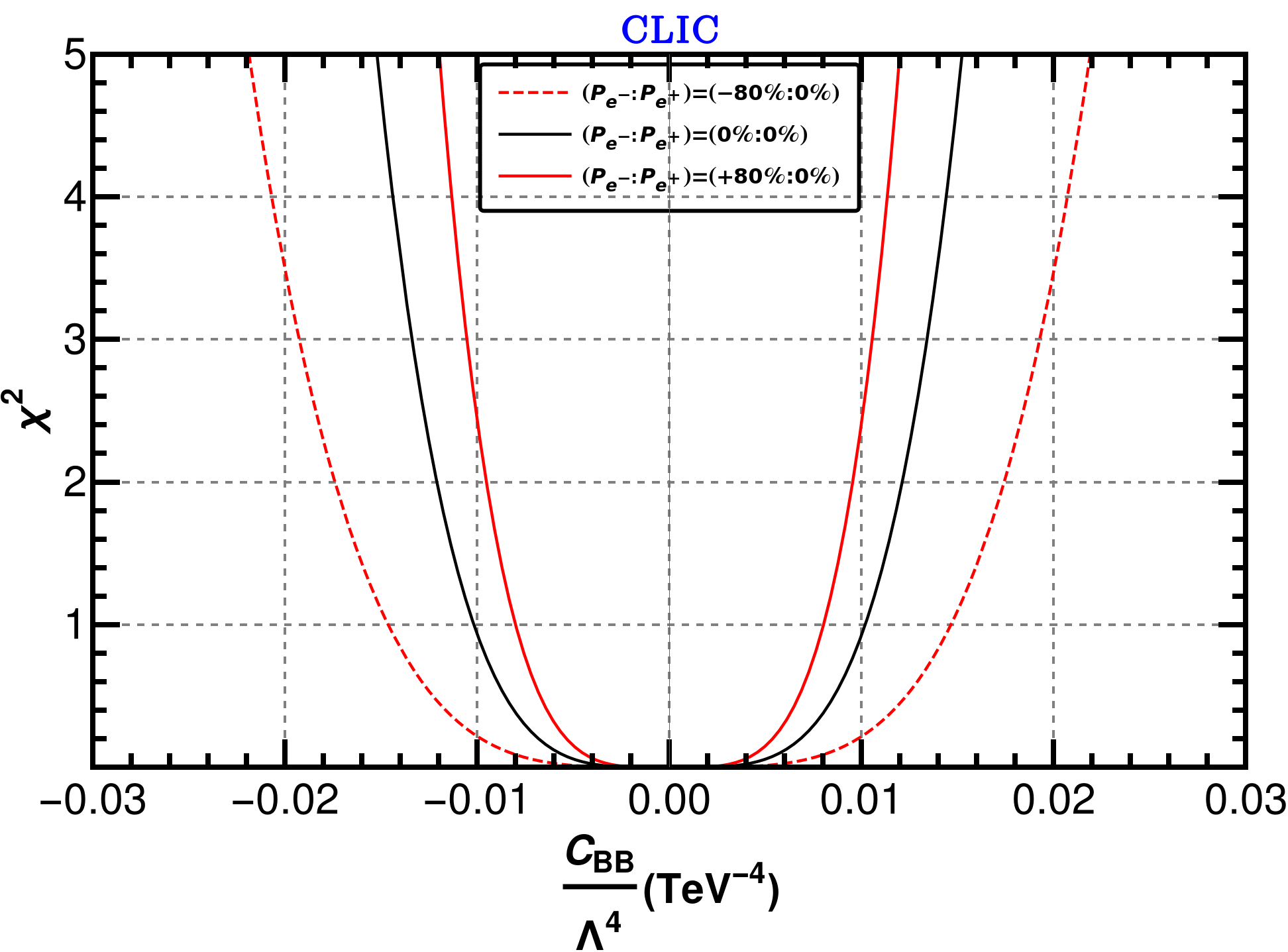
Using OOT, C.L. limit of NP couplings can be obtained from Eq. (23). We first consider = 1 TeV and 3 TeV with = 1000 and show 1-D as function of different NP couplings in the figure 5 and 6 respectively. While evaluating the in terms of one NP coupling, the other couplings are kept at zero. C.L. limit on the NP couplings has been tabulated in Table 2. We can see that, different NP couplings are sensitive to different choices of polarization combinations, because of unequal contribution of NP couplings to the various helicity amplitudes. We find that in case of ILC, for , and the best sensitivity is achieved with , whereas for , produces the best result. In context of CLIC, for we get best sensitivity for and for , and , the best sensitivity is obtained with . This phenomenon can be also understood from figure 4, where the contribution to production cross-section from is maximum in the polarization combination , whereas the other three couplings contribute maximally with . It is also evident that the initial beam polarization indeed enhances statistical precision in case of all four aNTGCs. In Table 2, we have quoted the statistical uncertainty (95% C.L) for all the aNTGC couplings for ILC and CLIC and make a comparison between the two. We can see that due to increased signal cross-section, CLIC yields better sensitivity compared to ILC at same integrated luminosity. The comparison between ILC, CLIC and ATLAS sensitivities will be discussed next.
  |
  |
  |
  |
| C.L. limit | ||||||
| Couplings | ILC | CLIC | ||||
   |
In figure 7, we compare the sensitivities achievable at ILC and CLIC with various polarizations and compare them with the limits obtained with the most recent ATLAS data ATLAS:2018nci. One can see that CLIC outperforms both LHC and ILC by at least an order of magnitude for all polarization combinations. However, in case of ILC, for , and polarization combination produce better sensitivity compared to ATLAS, whereas for , ILC sensitivities are better than that from ATLAS with . It is evident from the results that initial beam polarization can improve the level of precision in aNTGCs measurement to a large extent.
  |
   |
   |
In figure 8, we show the variation of statistical limits (95% C.L.) of the NP parameters with the integrated luminosity in the context of both ILC and CLIC. We have allowed the luminosity to vary from 10 to 1000 . With the increasing luminosity, the statistical limit of all the NP parameters is decreased and follow a similar trend. Varying the luminosity from 10 to 1000 enhances the statistical limits by 76% (64%), 69% (67%), 67% (65%), and 67% (64%) for , , , and , respectively for ILC (CLIC).
5.2 Correlation of CP-violating aNTGCs
Having discussed our results for each individual NP couplings, we will present our two-parameter analysis. The bounds shown in Figure 7 are the most conservative ones. However, there is a possibility that more than one non-zero couplings participate in process. For example, when CP-violation is considered, , and can contribute simultaneously in production and therefore, the sensitivity in measuring one coupling can be affected by the measurement of the other coupling. In order to capture this non-trivial correlation between these couplings, we have considered two aNTGCs non-zero at a time and computed the bound on the parameter space spanned by them. In figure 9, we show the statistical limits on two-parameters space spanned by , and respectively for different polarization combinations. Like one-parameter analysis, here too we can see that CLIC can offer precision at least one order of magnitude higher than that of ILC. Interestingly, we see non-trivial correlation between two parameters, which vary with varying degree of polarization. This happens due to non-trivial interference terms between various couplings. We see, unlike the one-parameter case, here even unpolarized beams can give rise to best sensitivity along certain coupling directions. Therefore, one can say, the two-parameter analysis can provide significantly different sensitivity and polarization-dependence, again owing its origin to the constructive or destructive interference.
In the context of ILC, we have considered the position beam to be both right and left polarized with same degree () whereas for CLIC the positron beam is unpolarized, while in both cases electron beam is supposed to have a higher degree of polarization (). Now, from figure 9, we can see that the is no significant change in the nature of correlation of aNTGCs in two-parameters space if we compare the elliptic contours between ILC and CLIC. However, the actual sizes of the contours will definitely depend on the degree of polarization. Therefore, one can infer that the correlation between two couplings will be dominantly governed by on electron beam polarization in case of both ILC and CLIC at the design polarization.
5.3 Sensitivity comparison: OOT vs cut-based analysis
In this section, we investigate the estimation of the sensitivity of aNTGCs through cut-based analysis and compare the results derived from OOT. The function for cut-based analysis is given by,
| (27) |
where and are the number of events from observation and theory in the bins of differential cross-section distribution after applying all the cuts described in section 4. The statistical uncertainty in bin is , assuming the number of events in each bin follows Poisson distribution. Now using cut-based analysis, we briefly discuss the measurement of only one dim-8 effective coupling. Therefore, we consider the most constrained dim-8 effective coupling among these four couplings. We again take up the design details of two linear colliders listed in Table 1 and show the 95% C.L. statistical limit of by the cyan color in the figure 10. The 95% C.L limits are tabulated in Table 3. The estimation of the sensitivity via OOT of is shown in magenta in the figure 10. Now, if we compare the sensitivity of dim-8 NP coupling, OOT outperforms cut-based analysis by a factor of 1.8. A detailed analysis in this regard is our future case of study.
   |
   |
| C.L. limit | ||||||
| Coupling | ILC | CLIC | ||||
We would like to reiterate that our analysis only involves non-zero effects from dimension-8 operators. However, the inclusion of loop-induced NP effects from dimension-6 operators contribute to production cross-section with of that of the tree-level results at CLIC ( TeV and TeV) and of the tree-level result at ILC (TeV and =1.3 TeV). Although the dominant contribution comes from dimension-8 operators, for especially the CLIC analysis, the effect of loop-effects from dimension-6 operators cannot be neglected. Having said that, in this work, we have obtained the maximum sensitivity that can be achieved for dimension-8 couplings (individual or pair-wise) while all the other couplings are assumed to be zero. The same approach has been taken in ATLAS:2018nci. The inclusion of all dimension-6 and 8 terms in a marginalized analysis will definitely weaken the limits obtained thus far. In fact, obtaining the best possible sensitivity for all the dimension-6 and -8 operators and taking in consideration all the relevant experimental results, can be the topic of a more elaborate future study.
6 Conclusion
In this work, we have considered dimension-8 operators, that are consistent with SM gauge group, using SMEFT framework, which can give rise to anomalous neutral triple gauge couplings, namely and . For this purpose, we have considered production at the linear colliders, the most suitable environment to study precision observables to probe physics beyond SM. We have analyzed mono-photon + missing energy as the final state signal and used useful kinematical cuts to segregate the signal from non-interfering SM backgrounds. In this context, missing energy () and missing transverse energy () play important role.
Next we have adopted optimal observable technique to find optimal sensitivity that can be achieved in the measurement of aNTGCs at the experiments. We have considered differential cross-section of production as the observable of optimal observable technique to estimate statistical limit on the aNTGCs which ensures that statistical limit are optimal in the sense that the covariance matrix is minimized. Using OOT, we have estimated the 95% C.L. limit on the dimension-8 aNTGCs. On one hand, we have performed individual one-dimensional analysis for all the couplings, on the other hand, the two-parameter analysis has also been performed in order to explore non-trivial correlation between different NP couplings. A comparative analysis of NP couplings between our predictions for future colliders, namely, ILC and CLIC and the most stringent limits obtained so far from ATLAS has been performed. While both linear colliders outperforms ATLAS with certain polarization combinations, CLIC offers at least ten times improvement over ILC sensitivities. For all the cases, the non-trivial effect of beam polarization can be noted. It is worthwhile to mention that different combination of polarized beams are sensitive to different couplings. Considering the choice of beam polarization that provides the most stringent limit at CLIC, we have observed that the optimal limit on dimension-8 aNTGCs are at least fifteen times better than the current experimental limit.
Acknowledgements.
The authors would like to thank Subhaditya Bhattacharya and Jose Wudka for useful discussions.References
- (1) L3 collaboration, Measurement of triple gauge boson couplings of the boson at LEP, Phys. Lett. B 586 (2004) 151 [hep-ex/0402036].
- (2) CMS collaboration, Measurement of the Cross Section in Collisions at TeV and Limits on Anomalous and Couplings, Eur. Phys. J. C 73 (2013) 2610 [1306.1126].
- (3) CMS collaboration, Search for anomalous triple gauge couplings in WW and WZ production in lepton + jet events in proton-proton collisions at 13 TeV, JHEP 12 (2019) 062 [1907.08354].
- (4) D. Choudhury and S. D. Rindani, Test of CP violating neutral gauge boson vertices in , Phys. Lett. B 335 (1994) 198 [hep-ph/9405242].
- (5) S. Atag and I. Sahin, and couplings at linear collider energies with the effects of Z polarization and initial state radiation, Phys. Rev. D 70 (2004) 053014 [hep-ph/0408163].
- (6) I. Ots, H. Uibo, H. Liivat, R. Saar and R. K. Loide, Possible anomalous and couplings and Z boson spin orientation in , Nucl. Phys. B 702 (2004) 346.
- (7) I. Ots, H. Uibo, H. Liivat, R. Saar and R. K. Loide, Possible anomalous and couplings and Z boson spin orientation in : The role of transverse polarization, Nucl. Phys. B 740 (2006) 212.
- (8) A. Gutierrez-Rodriguez, M. A. Hernandez-Ruiz and M. A. Perez, Probing the and Couplings Through the Process , Phys. Rev. D 80 (2009) 017301 [0808.0945].
- (9) B. Ananthanarayan, S. K. Garg, M. Patra and S. D. Rindani, Isolating CP-violating ZZ coupling in Z with transverse beam polarizations, Phys. Rev. D 85 (2012) 034006 [1104.3645].
- (10) B. Ananthanarayan, J. Lahiri, M. Patra and S. D. Rindani, New physics in at the ILC with polarized beams: explorations beyond conventional anomalous triple gauge boson couplings, JHEP 08 (2014) 124 [1404.4845].
- (11) R. Rahaman and R. K. Singh, On polarization parameters of spin-1 particles and anomalous couplings in , Eur. Phys. J. C 76 (2016) 539 [1604.06677].
- (12) R. Rahaman and R. K. Singh, On the choice of beam polarization in and anomalous triple gauge-boson couplings, Eur. Phys. J. C 77 (2017) 521 [1703.06437].
- (13) J. Ellis, S.-F. Ge, H.-J. He and R.-Q. Xiao, Probing the scale of new physics in the coupling at colliders, Chin. Phys. C 44 (2020) 063106 [1902.06631].
- (14) J. Ellis, H.-J. He and R.-Q. Xiao, Probing new physics in dimension-8 neutral gauge couplings at colliders, Sci. China Phys. Mech. Astron. 64 (2021) 221062 [2008.04298].
- (15) U. Baur and E. L. Berger, Probing the weak boson sector in production at hadron colliders, Phys. Rev. D 47 (1993) 4889.
- (16) J. Ellison and J. Wudka, Study of trilinear gauge boson couplings at the Tevatron collider, Ann. Rev. Nucl. Part. Sci. 48 (1998) 33 [hep-ph/9804322].
- (17) A. Senol, H. Denizli, A. Yilmaz, I. Turk Cakir, K. Y. Oyulmaz, O. Karadeniz et al., Probing the Effects of Dimension-eight Operators Describing Anomalous Neutral Triple Gauge Boson Interactions at FCC-hh, Nucl. Phys. B 935 (2018) 365 [1805.03475].
- (18) A. Yilmaz, A. Senol, H. Denizli, I. Turk Cakir and O. Cakir, Sensitivity on Anomalous Neutral Triple Gauge Couplings via Production at FCC-hh, Eur. Phys. J. C 80 (2020) 173 [1906.03911].
- (19) A. Senol, H. Denizli, A. Yilmaz, I. Turk Cakir and O. Cakir, The projections on and couplings via production in HL-LHC and HE-LHC, Phys. Lett. B 802 (2020) 135255 [1910.03843].
- (20) A. Yilmaz, Search for the limits on anomalous neutral triple gauge couplings via ZZ production in the channel at FCC-hh, Nucl. Phys. B 969 (2021) 115471 [2102.01989].
- (21) R. Rahaman and R. K. Singh, Anomalous triple gauge boson couplings in production at the LHC and the role of boson polarizations, Nucl. Phys. B 948 (2019) 114754 [1810.11657].
- (22) J. Ellis, H.-J. He and R.-Q. Xiao, Probing Neutral Triple Gauge Couplings at the LHC and Future Hadron Colliders, 2206.11676.
- (23) K. Hagiwara, R. D. Peccei, D. Zeppenfeld and K. Hikasa, Probing the Weak Boson Sector in , Nucl. Phys. B 282 (1987) 253.
- (24) F. M. Renard, Tests of Neutral Gauge Boson Selfcouplings With , Nucl. Phys. B 196 (1982) 93.
- (25) G. Gounaris, R. Kogerler and D. Schildknecht, ON DECAYS, Phys. Lett. B 137 (1984) 261.
- (26) G. Gounaris et al., Triple gauge boson couplings, in AGS / RHIC Users Annual Meeting, 1, 1996, hep-ph/9601233.
- (27) G. J. Gounaris, J. Layssac and F. M. Renard, Signatures of the anomalous and production at the lepton and hadron colliders, Phys. Rev. D 61 (2000) 073013 [hep-ph/9910395].
- (28) A. I. Hernández-Juárez, A. Moyotl and G. Tavares-Velasco, Contributions to () couplings from violating flavor changing couplings, Eur. Phys. J. C 81 (2021) 304 [2102.02197].
- (29) A. I. Hernández-Juárez and G. Tavares-Velasco, Non-diagonal contributions to vertex and bounds on couplings, 2203.16819.
- (30) H. Abramowicz et al., The International Linear Collider Technical Design Report - Volume 4: Detectors, 1306.6329.
- (31) CLIC accelerator collaboration, The Compact Linear Collider (CLIC) - Project Implementation Plan, 1903.08655.
- (32) ATLAS collaboration, Measurement of Wgamma and Zgamma production in proton-proton collisions at TeV with the ATLAS Detector, JHEP 09 (2011) 072 [1106.1592].
- (33) ATLAS collaboration, Measurements of and production in collisions at =7 TeV with the ATLAS detector at the LHC, Phys. Rev. D 87 (2013) 112003 [1302.1283].
- (34) CMS collaboration, Measurement of the Z Production Cross Section in pp Collisions at 8 TeV and Search for Anomalous Triple Gauge Boson Couplings, JHEP 04 (2015) 164 [1502.05664].
- (35) CMS collaboration, Measurement of the production cross section in pp collisions at 8 TeV and limits on anomalous and trilinear gauge boson couplings, Phys. Lett. B 760 (2016) 448 [1602.07152].
- (36) ATLAS collaboration, Measurement of the production cross section in pp collisions at TeV with the ATLAS detector and limits on anomalous triple gauge-boson couplings, JHEP 12 (2018) 010 [1810.04995].
- (37) L3 collaboration, Study of the process at LEP and limits on triple neutral-gauge-boson couplings, Phys. Lett. B 597 (2004) 119 [hep-ex/0407012].
- (38) OPAL collaboration, Study of Z pair production and anomalous couplings in collisions at between 190-GeV and 209-GeV, Eur. Phys. J. C 32 (2003) 303 [hep-ex/0310013].
- (39) D. Atwood and A. Soni, Analysis for magnetic moment and electric dipole moment form-factors of the top quark via , Phys. Rev. D 45 (1992) 2405.
- (40) M. Davier, L. Duflot, F. Le Diberder and A. Rouge, The Optimal method for the measurement of tau polarization, Phys. Lett. B 306 (1993) 411.
- (41) M. Diehl and O. Nachtmann, Optimal observables for the measurement of three gauge boson couplings in — , Z. Phys. C 62 (1994) 397.
- (42) J. F. Gunion, B. Grzadkowski and X.-G. He, Determining the and couplings of a neutral Higgs boson of arbitrary CP nature at the NLC, Phys. Rev. Lett. 77 (1996) 5172 [hep-ph/9605326].
- (43) K. Hagiwara, S. Ishihara, J. Kamoshita and B. A. Kniehl, Prospects of measuring general Higgs couplings at e+ e- linear colliders, Eur. Phys. J. C 14 (2000) 457 [hep-ph/0002043].
- (44) S. Dutta, K. Hagiwara and Y. Matsumoto, Measuring the Higgs-Vector boson Couplings at Linear Collider, Phys. Rev. D 78 (2008) 115016 [0808.0477].
- (45) B. Grzadkowski and Z. Hioki, CP violating lepton energy correlation in , Phys. Lett. B 391 (1997) 172 [hep-ph/9608306].
- (46) B. Grzadkowski, Z. Hioki and M. Szafranski, Four Fermi effective operators in top quark production and decay, Phys. Rev. D 58 (1998) 035002 [hep-ph/9712357].
- (47) B. Grzadkowski and Z. Hioki, Probing top quark couplings at polarized NLC, Phys. Rev. D 61 (2000) 014013 [hep-ph/9805318].
- (48) B. Grzadkowski and J. Pliszka, Testing top quark Yukawa interactions in , Phys. Rev. D 60 (1999) 115018 [hep-ph/9907206].
- (49) B. Grzadkowski and Z. Hioki, Optimal observable analysis of the angular and energy distributions for top quark decay products at polarized linear colliders, Nucl. Phys. B 585 (2000) 3 [hep-ph/0004223].
- (50) B. Grzadkowski, Z. Hioki, K. Ohkuma and J. Wudka, Probing anomalous top quark couplings induced by dimension-six operators at photon colliders, Nucl. Phys. B 689 (2004) 108 [hep-ph/0310159].
- (51) B. Grzadkowski, Z. Hioki, K. Ohkuma and J. Wudka, Optimal-observable analysis of possible new physics using the b quark in — — , Phys. Lett. B 593 (2004) 189 [hep-ph/0403174].
- (52) B. Grzadkowski, Z. Hioki, K. Ohkuma and J. Wudka, Optimal beam polarizations for new-physics search through — — , JHEP 11 (2005) 029 [hep-ph/0508183].
- (53) J. F. Gunion and J. Pliszka, Determining the relative size of the CP even and CP odd Higgs boson couplings to a fermion at the LHC, Phys. Lett. B 444 (1998) 136 [hep-ph/9809306].
- (54) Z. Hioki, T. Konishi and K. Ohkuma, Studying possible CP-violating Higgs couplings through top-quark pair productions at muon colliders, JHEP 07 (2007) 082 [0706.4346].
- (55) Q.-H. Cao and J. Wudka, Search for new physics via single top production at TeV energy colliders, Phys. Rev. D 74 (2006) 094015 [hep-ph/0608331].
- (56) S. Bhattacharya, S. Jahedi and J. Wudka, Probing heavy charged fermions at collider using the optimal observable technique, JHEP 05 (2022) 009 [2106.02846].
- (57) S. Bhattacharya, S. Nandi and S. K. Patra, Optimal-observable analysis of possible new physics in , Phys. Rev. D 93 (2016) 034011 [1509.07259].
- (58) Z. Calcuttawala, A. Kundu, S. Nandi and S. K. Patra, Optimal observable analysis for the decay plus missing energy, Eur. Phys. J. C 77 (2017) 650 [1702.06679].
- (59) Z. Calcuttawala, A. Kundu, S. Nandi and S. Kumar Patra, New physics with the lepton flavor violating decay , Phys. Rev. D 97 (2018) 095009 [1802.09218].
- (60) W. Buchmuller and D. Wyler, Effective Lagrangian Analysis of New Interactions and Flavor Conservation, Nucl. Phys. B 268 (1986) 621.
- (61) B. Grzadkowski, M. Iskrzynski, M. Misiak and J. Rosiek, Dimension-Six Terms in the Standard Model Lagrangian, JHEP 10 (2010) 085 [1008.4884].
- (62) L. Lehman, Extending the Standard Model Effective Field Theory with the Complete Set of Dimension-7 Operators, Phys. Rev. D 90 (2014) 125023 [1410.4193].
- (63) S. Bhattacharya and J. Wudka, Dimension-seven operators in the standard model with right handed neutrinos, Phys. Rev. D 94 (2016) 055022 [1505.05264].
- (64) C. W. Murphy, Dimension-8 operators in the Standard Model Eective Field Theory, JHEP 10 (2020) 174 [2005.00059].
- (65) H.-L. Li, Z. Ren, J. Shu, M.-L. Xiao, J.-H. Yu and Y.-H. Zheng, Complete set of dimension-eight operators in the standard model effective field theory, Phys. Rev. D 104 (2021) 015026 [2005.00008].
- (66) Particle Data Group collaboration, Review of Particle Physics, PTEP 2022 (2022) 083C01.
- (67) C. Degrande, A basis of dimension-eight operators for anomalous neutral triple gauge boson interactions, JHEP 02 (2014) 101 [1308.6323].
- (68) J. Alwall, R. Frederix, S. Frixione, V. Hirschi, F. Maltoni, O. Mattelaer et al., The automated computation of tree-level and next-to-leading order differential cross sections, and their matching to parton shower simulations, JHEP 07 (2014) 079 [1405.0301].
- (69) DELPHES 3 collaboration, DELPHES 3, A modular framework for fast simulation of a generic collider experiment, JHEP 02 (2014) 057 [1307.6346].
- (70) N. D. Christensen and C. Duhr, FeynRules - Feynman rules made easy, Comput. Phys. Commun. 180 (2009) 1614 [0806.4194].