跳到论文正文
W Papers独立论文阅读器 arXiv:2212.04924 论文正文 计算阅读时间 · 0%
引用这篇论文根据当前论文元数据生成,正式投稿前建议核对。


License: CC BY 4.0
arXiv:2212.04924v2 [quant-ph] 21 Dec 2023

Quantum advantage and stability to errors in analogue quantum simulators

Rahul Trivedi Thanks: Both authors contributed equally. Affiliation: Max-Planck-Institut für Quantenoptik, Hans-Kopfermann-Str. 1, 85748 Garching, Germany. Affiliation: Munich Center for Quantum Science and Technology (MCQST), Schellingstr. 4, D-80799 Munich, Germany. Affiliation: Electrical and Computer Engineering, University of Washington, Seattle, WA - 98195, USA    Adrian Franco Rubio Thanks: Both authors contributed equally. Affiliation: Max-Planck-Institut für Quantenoptik, Hans-Kopfermann-Str. 1, 85748 Garching, Germany. Affiliation: Munich Center for Quantum Science and Technology (MCQST), Schellingstr. 4, D-80799 Munich, Germany.    J. Ignacio Cirac Affiliation: Max-Planck-Institut für Quantenoptik, Hans-Kopfermann-Str. 1, 85748 Garching, Germany. Affiliation: Munich Center for Quantum Science and Technology (MCQST), Schellingstr. 4, D-80799 Munich, Germany.
August 11, 2026
Abstract

Several quantum hardware platforms, while being unable to perform fully fault-tolerant quantum computation, can still be operated as analogue quantum simulators for addressing many-body problems. However, due to the presence of errors, it is not clear to what extent those devices can provide us with an advantage with respect to classical computers. In this work we consider the use of noisy analogue quantum simulators for computing physically relevant properties of many-body systems both in equilibrium and undergoing dynamics. We first formulate a system-size independent notion of stability against extensive errors, which we prove for Gaussian fermion models, as well as for a restricted class of spin systems. Remarkably, for the Gaussian fermion models, our analysis shows the stability of critical models which have long-range correlations. Furthermore, we analyze how this stability may lead to a quantum advantage, for the problem of computing the thermodynamic limit of many-body models, in the presence of a constant error rate and without any explicit error correction.

Quantum information processing systems hold the promise of solving a number of problems in physics and computer science faster than their classical counterparts Jozsa 2001; Montanaro 2016. However, most quantum algorithms with theoretical performance guarantees require a fault-tolerant quantum computer Aharonov et al. 1996; Aharonov and Ben-Or 1997; Aharonov et al. 2006. While in principle possible, implementing a fault tolerant quantum computer is a technological challenge that could still take a long time to solve. This has motivated several investigations trying to identify both quantum algorithms, as well as physically relevant computational problems, that can be addressed by quantum hardware in the near term and without any explicit error correction.

Analog quantum simulators, wherein a target Hamiltonian is mimicked by an experimentally controllable system, have shown some promise in solving problems arising in many-body physics in the near term Altman et al. 2021; Daley et al. 2022; Cirac and Zoller 2012. A typical analogue quantum simulator, while not necessarily being able to perform an arbitrary computation, would instead aim to approximately implement a relevant spatially-local Hamiltonian, HH. In several many-body problems, HH can additionally be taken to be translationally invariant. The quantum simulator can then be used to prepare a physically relevant quantum state ρH\rho_{H} associated with the Hamiltonian HH, such as its ground state, Gibbs state or a state produced under dynamics. In a typical quantum simulation experiment, we would then measure the expectation value of an intensive observable OO, which is either often a local observable at a single site on the lattice or a correlation function, i.e. a product of local observables at a few sites. Examples of such Hamiltonians and observables can be found in a variety of problems in physics — for e.g. in study of correlated electronic systems Zhou et al. 2021; Stormer et al. 1999; Broholm et al. 2020; Qin et al. 2022, quantum spin systems Spalek 2007; Mi et al. 2022; Chen et al. 2022; Pal and Huse 2010; Vosk et al. 2015 as well as lattice-gauge theories Rothe 2012; Kogut 1983. Furthermore, there have been several proposals to implement quantum simulation of these models in different hardware platforms, such as cold atoms in optical lattices, trapped ion systems or superconducting qubits Esslinger 2010; Houck et al. 2012; Porras and Cirac 2004; Blatt and Roos 2012; Garcia-Ripoll et al. 2004; Zohar et al. 2015; Zohar et al. 2012; Zohar et al. 2013; Banuls et al. 2020.

Practically, quantum simulators offer several distinct advantages in solving many-body problems as opposed to general purpose quantum computers. First, quantum simulators aim to solve only a much smaller and specialized set of problems, and thus have much milder hardware requirements than a universal quantum computer. Furthermore, quantum simulators are more naturally suited to many-body problems, since they avoid a Hamiltonian-to-circuit mapping for e.g. by trotterizing the evolution into a quantum circuit, which typically incurs in a rapid proliferation of errors Cirac and Zoller 2012; Stilck França and Garcia-Patron 2021; De Palma et al. 2022; González-García et al. 2022; Daley et al. 2022. Furthermore, since the observables of interest are typically local intensive observables, we expect them to be somewhat more robust to errors even if the global quantum state of the simulator is very sensitive. These expectations make quantum simulators very promising in providing some advantage with respect to classical computers when addressing typical quantum many-body physics problems.

However, developing rigorous criteria to outline the quantum advantage of a quantum simulator runs into several theoretical issues. First, quantum simulators do not implement any error correction and typically simulate many-body physics in the presence of noise. While several previous works have theoretically outlined the computational power of quantum simulators by developing the notion of a universal quantum simulator Kraus et al. 2007; Cubitt et al. 2018; Zhou and Aharonov 2021 and rigorously established the possibility of quantum advantage without noise, the presence of experimentally realistic noise has to be carefully accounted for in understanding their utility in many-body problems. Second, since quantum simulators are usually devoted to analyzing intensive observables, and in many-body physics we are typically interested in the thermodynamic limit of such observables, we need to revisit the usual notion of quantum advantage. In particular, instead of characterizing the quantum and classical effort required to compute the many-body observable as a function of the system size, which is not meaningful in the thermodynamic limit, we can characterize the effort required to compute the many-body intensive observable within a user-specific precision of the thermodynamic limit Aharonov and Irani 2022; Watson and Cubitt 2022. In this paper, we address both of these issues — we provide evidence that many physically relevant critical and non-critical many-body models are stable to errors in the quantum simulators. Importantly, even without error correction, we can use a quantum simulator to determine the thermodynamic limits of intensive observables in these problems to a hardware-limited precision. Furthermore, we also propose a notion of quantum advantage, in the presence of errors, for such problems, where the figure of merit is the computational time to obtain an intensive quantity in the thermodynamic limit to a hardware-limited precision. By providing explicit lower bounds on certifiable classical algorithms for the many-body problems that we consider, we provide evidence that quantum simulators can possibly provide superpolynomial to exponential quantum advantage over rigorous classical algorithms even without error correction.

I Stable quantum simulation tasks

I.1 General setup

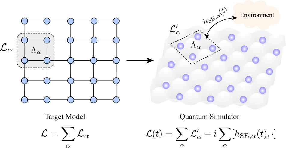
To keep our analysis general, we will consider quantum simulators for solving both closed system (i.e. implementing a Hamiltonian) as well as open system (i.e. implementing a Lindbladian) many-body problems. Suppose that the quantum simulator was trying to configure a spatially local Lindbladian ℒ\mathcal{L} given by

ℒ=∑αℒα,\displaystyle\mathcal{L}=\sum_{\alpha}\mathcal{L}_{\alpha}, (1)

where ℒα\mathcal{L}_{\alpha} is a Lindbladian acting on spins within a local region Λα\Lambda_{\alpha}. For translationally invariant problems, the superoperator ℒα\mathcal{L}_{\alpha} would additionally be independent of Λα\Lambda_{\alpha}, and for closed system problems, we can assume ℒα=−i⁡[hα,⋅]\mathcal{L}_{\alpha}=-i[h_{\alpha},\cdot] for some operator hαh_{\alpha} supported on Λα\Lambda_{\alpha}. The quantum simulator would, in general, suffer from coherent errors in the configured Lindbladian as well as incoherent errors arising due to its interaction with an external environment. To account for these errors, we model the ‘implemented’ Hamiltonian on the quantum simulator by

ℒ′(t)=∑Λ(ℒα′−i[hSE,α(t),⋅],).\displaystyle\mathcal{L}^{\prime}(t)=\sum_{\Lambda}\bigg(\mathcal{L}_{\alpha}^{\prime}-i[h_{\text{SE},\alpha}(t),\cdot],\bigg). (2a)
Here ℒα′−ℒα\mathcal{L}_{\alpha}^{\prime}-\mathcal{L}_{\alpha} is an error in the Lindbladian implemented on spins in Λα\Lambda_{\alpha} — this can arise either from configuration errors in the Hamiltonian and the jump operators corresponding to ℒα\mathcal{L}_{\alpha}, or from incoherent errors that can be well approximated as Markovian. Furthermore, we also consider the possibility of non-Markovian incoherent errors — these are captured by hSE,α​(t)h_{\text{SE},\alpha}(t), which accounts for the interaction of the spins in the region Λα\Lambda_{\alpha} with an external environment (in the interaction picture with respect to the environment). For concreteness, we will model the decohering environment as a Gaussian environment and assume that
hSE,α​(t)=∑j=1nLAj,α​(t)​Qj,α†+h.c.,\displaystyle h_{\text{SE},\alpha}(t)=\sum_{j=1}^{n_{L}}A_{j,\alpha}(t)Q_{j,\alpha}^{\dagger}+\text{h.c.}, (2b)

where Q1,α,Q2,α​…​QnL,αQ_{1,\alpha},Q_{2,\alpha}\dots Q_{n_{L},\alpha} are the jump operators, each supported on Λα\Lambda_{\alpha}, through which the spins in Λα\Lambda_{\alpha} interact with a decohering environment, and A1,α​(t),A2,α​(t)​…​AnL,α​(t)A_{1,\alpha}(t),A_{2,\alpha}(t)\dots A_{n_{L},\alpha}(t) are annihilation operators for the environment. We assume that [Aj,α​(t),Aj′,α′†​(t′)]=δα,α′​δj,j′​Kj,α​(t−t′)[A_{j,\alpha}(t),A_{j^{\prime},\alpha^{\prime}}^{\dagger}(t^{\prime})]=\delta_{\alpha,\alpha^{\prime}}\delta_{j,j^{\prime}}K_{j,\alpha}(t-t^{\prime}) for bosonic environments or {Aj,α​(t),Aj′,α′†​(t′)}=δα,α′​δj,j′​Kj,α​(t−t′)\{A_{j,\alpha}(t),A_{j^{\prime},\alpha^{\prime}}^{\dagger}(t^{\prime})\}=\delta_{\alpha,\alpha^{\prime}}\delta_{j,j^{\prime}}K_{j,\alpha}(t-t^{\prime}) for fermionic environments and we choose the normalization of Qj,αQ_{j,\alpha} such that ∫ℝ|Kj,α​(τ)|​𝑑τ=1\int_{\mathbb{R}}|{K_{j,\alpha}(\tau)}|d\tau=1. The function Kj,α​(τ)K_{j,\alpha}(\tau) can be understood as the memory kernel corresponding to the non-Markovian system-environment interaction. In particular and not unexpectedly, choosing Kj,α​(τ)=δ​(τ)K_{j,\alpha}(\tau)=\delta(\tau) would yield a Markovian master equation for an environment initially in the vacuum state.

We introduce a parameter δ\delta such that ‖ℒα′−ℒα‖⋄≤δ\|{\mathcal{L}_{\alpha}^{\prime}-\mathcal{L}_{\alpha}}\|_{\diamond}\leq\delta and ‖Qj,α‖≤δ\|{Q_{j,\alpha}}\|\leq\sqrt{\delta} — the parameter δ\delta can be considered to be the “hardware error rate” in the quantum simulator. A well designed experimental setup can, in principle, achieve δ≪1\delta\ll 1 — however, since there are an extensive number of errors in the simulator, we generically expect the state of the simulator to be at a distance of δ×n\delta\times n from the target state. In the worst case, this would imply that the results of the quantum simulator can only be trusted when δ<o⁡(1/n)\delta<o(1/n), and this would limit their applicability to small-scale problems. Importantly, for applications of quantum simulators to problems in many-body physics, this would imply that noisy quantum simulators, in the worst case, cannot be used to faithfully capture thermodynamic limits (i.e. n→∞n\to\infty).

Refer to caption
Figure 1: Schematic depiction of our error model for analogue quantum simulator. A target Lindbladian ℒ\mathcal{L}, expressed as sum of Lindbladian terms modelling interactions between groups of spins, when implemented on an analogue quantum simulator would have an hardware error per qubit — this error can either be due to an incorrect configuration of the Lindbladian (i.e. implementing ℒα′\mathcal{L}_{\alpha}^{\prime} instead of ℒα\mathcal{L}_{\alpha}) or due to interaction with an external decohering environment.

An alternative viewpoint would be to ask if there are certain interesting many-body problems for which a good estimate for the thermodynamic limit can be produced with a hardware with constant errors. This motivates us to look for ‘quantum simulation tasks’ which are stable to these extensive errors, as made precise in the following definition.

Definition 1 (Stable quantum simulation task).

The quantum simulation task on nn spins of measuring an observable OO in a state ρℒ\rho_{\mathcal{L}} associated with a target Lindbladian ℒ\mathcal{L} is said to be stable if the corresponding state ρℒ′\rho^{\prime}_{\mathcal{L}} prepared by the noisy simulator satisfies

|Tr​(O​ρ)−Tr​(O​ρ′)|≤f⁡(δ),|{\textnormal{Tr}(O\rho)-\textnormal{Tr}(O\rho^{\prime})}|\leq f(\delta),

for some ff, independent of nn, such that f⁡(δ)→0f(\delta)\to 0 as δ→0\delta\to 0.

If a quantum simulation task is stable as per this definition, we can hope to be able to estimate the thermodynamic limit of the observable on a quantum simulator to a precision limited only by the hardware error rate δ\delta, and independent of the size of the problem. In particular, these problems would not require the hardware error to be scaled down with system size even in the absence of error correction, and it is reasonable to consider them to be problems that analogue quantum simulators can conceivably solve in the near term.

In the remainder of this section, we systematically study several important problems arising in many-body physics, and show that commonly considered intensive observables are expected to be stable to errors. We first study geometrically local Gaussian fermion models with Gaussian errors, and show that intensive observables (either local observables, or translationally invariant sums of local observables) are stable both for the problem of constant-time dynamics and equilibrium without any restrictive assumptions on the model — our results hold not only for gapped models, but also for gapless models. Then, we study the same question for (non-Gaussian) many-body spin systems — here, we use well known locality properties of these models to show that local observables are stable for constant-time dynamics and equilibrium properties, but with more restrictive assumptions on the system (e.g. the Hamiltonian being stably gapped for ground states, or exhibiting exponential clustering of correlations in the Gibbs state). Our results are summarized in Table 1, and lend strong evidence for several many-body problems being amenable to noisy quantum simulation.

Problem Error Assumption Observable Stability, f⁡(δ)f(\delta)
Dynamics General errors GF: None.


SS: None.
GF: kk-local observables.

SS: Local observables.
GF: O⁡(δ​t)O(\delta t).


SS: O⁡(δ​td+1)O(\delta t^{d+1}).
Ground state Coherent Hamiltonian errors GF: Assumption 1.


SS: Stable gap.
GF: Translationally invariant k−k-local observables

SS: Local observables.
GF: O⁡(δβ)O(\delta^{\beta}), where β\beta is a model dependent constant.

SS: O⁡(δ)O(\delta).
Gibbs state Coherent Hamiltonian errors GF: No assumption.


SS: Stably exponentially clustered correlations.
GF: Translationally invariant k−k-local observables.

SS: Local observables.
GF: O⁡(δ)O(\sqrt{\delta}).


SS: O~​(exp⁡(−Ω⁡(log1/d⁡δ−1)))\tilde{O}(\exp(-\Omega(\log^{1/d}{\delta^{-1}}))).
Fixed points GF: Coherent and Incoherent Markovian errors.

SS: General errors
GF: Assumption 2.


SS: Rapid Mixing.
GF: Translationally invariant k−k-local observables


SS: Local observables
.
GF: O⁡(δβ)O(\delta^{\beta}), where β\beta is a model dependent constant.


SS: O⁡(δ)O(\delta).
Table 1: Summary of the stability results for dynamical and equilibrium many-body problems, together with the required assumptions on the many-body model and errors. Both results for Gaussian fermions and spin systems are summarized — ‘GF’ indicates Gaussian fermions and ‘SS’ indicates spin systems. Note that observables for the Gaussian fermionic problems are all quadratic. Also, O~\tilde{O} in the first column suppresses log⁡(δ−1)\log(\delta^{-1}) factors.

I.2 Gaussian fermion models

We will consider fermions arranged on a d−d-dimensional lattice with LL sites in each direction ℤLd\mathbb{Z}_{L}^{d}, and at each site we have DD fermionic modes — we denote by cxαc_{x}^{\alpha} for x∈ℤLd,α∈{1,2​…​2​D}x\in\mathbb{Z}_{L}^{d},\alpha\in\{1,2\dots 2D\} the Majorana operators associated with each site xx. We consider a general open quantum simulation problem with geometrically local interactions with interaction range RR. This is specified by a quadratic Hamiltonian HH, and nLn_{L} linear jump operators Lj,xL_{j,x} for every site x∈ℤLdx\in\mathbb{Z}_{L}^{d},

H=∑x,y∈ℤLdd⁡(x,y)≤R∑α,β=12​Dhx,yα,β​cxα​cyβ,\displaystyle H=\sum_{\begin{subarray}{c}x,y\in\mathbb{Z}_{L}^{d}\\ d(x,y)\leq R\end{subarray}}\sum_{\alpha,\beta=1}^{2D}h^{\alpha,\beta}_{x,y}c_{x}^{\alpha}c_{y}^{\beta}, (3a)
Lj,x=∑y∈ℤLdd⁡(x,y)≤R∑α=12​Dlj;x,yα​cyα,∀j∈{1,2​…​nL}.\displaystyle L_{j,x}=\sum_{\begin{subarray}{c}y\in\mathbb{Z}_{L}^{d}\\ d(x,y)\leq R\end{subarray}}\sum_{\alpha=1}^{2D}l_{j;x,y}^{\alpha}c_{y}^{\alpha},\forall\ j\in\{1,2\dots n_{L}\}. (3b)

Without loss of generality, we can assume that |hx,yα,β|≤1|h^{\alpha,\beta}_{x,y}|\leq 1, |lj;x,yα|≤1|{l_{j;x,y}^{\alpha}}|\leq 1 and nL≤2​D​(2​R+1)dn_{L}\leq 2D(2R+1)^{d}.

For the results in this subsection, we restrict ourselves to Gaussian errors (coherent or incoherent) when this model is implemented on a quantum simulator. Due to coherent hardware errors, the quantum simulator instead implements a perturbed free-fermion Hamiltonian H′H^{\prime},

H′=∑x,y∈ℤLdd⁡(x,y)≤R∑α,β=12​Dhx,y′α,β​cxα​cyβ,H^{\prime}=\sum_{\begin{subarray}{c}x,y\in\mathbb{Z}_{L}^{d}\\ d(x,y)\leq R\end{subarray}}\sum_{\alpha,\beta=1}^{2D}h^{\prime\alpha,\beta}_{x,y}c_{x}^{\alpha}c_{y}^{\beta}, (4a)
such that |hx,yα,β−hx,y′α,β|≤δ|{h^{\alpha,\beta}_{x,y}-h^{\prime\alpha,\beta}_{x,y}}|\leq\delta. Furthermore, due to errors in the configuration of the jump operators, or due to Markovian incoherent errors, the quantum simulator implements perturbed jump operators Lj,x′L_{j,x}^{\prime},
Lj,x′=∑y∈ℤLdd⁡(x,y)≤R∑α=12​Dlj;x,y′α​cyα,∀j∈{1,2​…​nL}.L_{j,x}^{\prime}=\sum_{\begin{subarray}{c}y\in\mathbb{Z}_{L}^{d}\\ d(x,y)\leq R\end{subarray}}\sum_{\alpha=1}^{2D}l^{\prime\alpha}_{j;x,y}c_{y}^{\alpha},\ \forall\ j\in\{1,2\dots n_{L}\}. (4b)

where again |lj;x,yα−lj;x,y′α|≤δ|{l_{j;x,y}^{\alpha}-l^{\prime\alpha}_{j;x,y}}|\leq\delta. Furthermore, we also consider Gaussian incoherent interactions with a decohering environment which, following the general setup described previously, is captured by a Gaussian system-environment HSE​(t)=∑x∈ℤLdhx,SE​(t)H_{\text{SE}}(t)=\sum_{x\in\mathbb{Z}_{L}^{d}}h_{x,\text{SE}}(t) with

hx,SE​(t)=∑j=1nLAj,x​(t)​Qj,x†+h.c..\displaystyle h_{x,\text{SE}}(t)=\sum_{j=1}^{n_{L}}A_{j,x}(t)Q_{j,x}^{\dagger}+\text{h.c.}. (5a)
Here
Qj,x=∑y∈ℤLdd⁡(x,y)≤Rqj,x;yα​cyα,\displaystyle Q_{j,x}=\sum_{\begin{subarray}{c}y\in\mathbb{Z}_{L}^{d}\\ d(x,y)\leq R\end{subarray}}q_{j,x;y}^{\alpha}c_{y}^{\alpha}, (5b)

with |qj,x;yα|≤δ|{q_{j,x;y}^{\alpha}}|\leq\sqrt{\delta} and Ax​(t)A_{x}(t) is an annihilation operator in the fermionic environment coupling to sites in the neighbourhood of xx. These annihilation operators satisfy {Ax​(t),Ax′†​(s)}=δx,x′​Kx​(t−s)\{A_{x}(t),A_{x^{\prime}}^{\dagger}(s)\}=\delta_{x,x^{\prime}}K_{x}(t-s), where Kx​(τ)K_{x}(\tau) is the memory kernel describing the system-environment interaction and is assumed to satisfy ∫ℝ|Kx​(τ)|​𝑑τ≤1\int_{\mathbb{R}}|{K_{x}(\tau)}|d\tau\leq 1.

Finite-time dynamics. We first consider the problem of evolving the quantum simulator for time tt and measure the expectation value of Gaussian observables O0O_{0} which are either k−k-local, i.e. they act on a set 𝒮⊆ℤLd\mathcal{S}\subseteq\mathbb{Z}_{L}^{d} of kk sites

O0=∑x,y∈𝒮∑α,β=12​Dox,yα,β​cxα​cyβ,\displaystyle O_{0}=\sum_{x,y\in\mathcal{S}}\sum_{\alpha,\beta=1}^{2D}o_{x,y}^{\alpha,\beta}c_{x}^{\alpha}c_{y}^{\beta}, (6)

or weighted averages of k−k-local Gaussian observables i.e. are of the form ∑i=1Mwi​Oi\sum_{i=1}^{M}w_{i}O_{i}, where OiO_{i} is of the form Eq. 6, ∑i=1M|wi|=1\sum_{i=1}^{M}|{w_{i}}|=1 and MM can possibly grow with n=D​Ldn=DL^{d}. We consider an arbitrary Gaussian initial state, and let the target state ρ\rho be the state obtained by evolving it with the target Lindbladian specified by Eq. 3 for time tt. We show in Appendix B.1 that

Proposition 1.

The quantum simulation task of measuring k−k-local Gaussian observables, or their weighted sums, after constant-time dynamics under a spatially local Gaussian Hamiltonian is stable to coherent and incoherent errors with f⁡(δ)=O⁡(t​δ)f(\delta)=O(t\delta).

We point out that the dependence of the error between the observable in perturbed and unperturbed models on tt is independent of the dimensionality of the lattice dd — this result is thus stronger than what would be expected simply from locality, wherein the error would be expected to grow as t×(Number of sites in the light cone at time ​t)∝td+1t\times(\text{Number of sites in the light cone at time }t)\propto t^{d+1} — we revisit this in section IV.

Equilibrium. We next study the stability properties of intensive observables in equilibrium. For simplicity, we first consider the closed-system setting and study the stability of the ground state and Gibbs state. Suppose that the quantum simulator implements a target geometrically local Hamiltonian (Eq. 3a), but due to the presence of coherent errors instead configures a perturbed Hamiltonian H′H^{\prime} (Eq. 4a). We emphasize that we only consider the simpler coherent Hamiltonian errors while studying the stability of ground state and Gibbs state, since these states can only be meaningfully defined for a closed system. Later on in this section, we will study the more natural equilibrium problem of the ‘Lindbladian fixed point’ where incoherent errors can also be accounted for. Furthermore, we make the following additional physically reasonable assumption on the density of modes of the target Hamiltonian HH.

Assumption 1.

The number of eigenfrequencies nηn_{\eta} of HH, which are eigenvalues of the matrix hx,yα,βh_{x,y}^{\alpha,\beta} defining the target Hamiltonian, lying in the interval [−η,η][-\eta,\eta] for sufficiently small η\eta satisfy the upper bound

nη≤n​fh​(η)+κ⁡(η,n),\displaystyle n_{\eta}\leq nf_{h}(\eta)+\kappa(\eta,n), (7)

where n=D​Ldn=DL^{d} is the number of fermionic modes, fh​(η)≤O⁡(ηα)f_{h}(\eta)\leq O(\eta^{\alpha}) for some α>0\alpha>0 and κ⁡(η,n)\kappa(\eta,n) is o⁡(n)o(n) for any fixed η\eta.

Alternatively stated, this assumption is a continuity11 1 More precisely, it demands that limn→∞nη/n\lim_{n\to\infty}n_{\eta}/n is a Hölder continuous function of η\eta. condition on the thermodynamic limit of the fraction of eigenmodes with energies in the interval [−η,η][-\eta,\eta] and it ensures that eigenvalues do not accumulate too fast near zero. It is expected to be true for most physically relevant models — in particular, it is weaker than the existence of a gap and thus contains gapped models, which are well known to exist for many experimentally relevant many-body problems. For a gapped Gaussian fermionic model, fh​(η)=0f_{h}(\eta)=0 since, if there are fermionic eigenmodes near 00, then adding a fermion into these modes would provide an excited state with only O⁡(n−1)O(n^{-1}) energy higher than the ground state energy. Furthermore, we also expect this assumption to be generically true for translationally invariant local Hamiltonians, where the eigenfrequencies can be described by a smooth dispersion relation ω⁡(k)\omega(k) as a function of the momentum kk associated with that mode. In this case, fh​(η)≤O⁡(ηα)f_{h}(\eta)\leq O(\eta^{\alpha}), with α\alpha being determined by the derivatives of ω⁡(k)\omega(k) in the vicinity of ω=0\omega=0.

The observables we consider while analyzing ground states are translationally invariant Gaussian observables generated k−k-locally, i.e., if O0O_{0} is a k−k-local observable of the form of Eq. 6, then we consider observables of the form

O=1n​∑x∈ℤLdτx​(O0),O=\frac{1}{n}\sum_{x\in\mathbb{Z}_{L}^{d}}\tau_{x}(O_{0}),

where τx​(O0)\tau_{x}(O_{0}) is the observable O0O_{0} translated by xx. Considering the target state to be the ground state of the Gaussian fermion Hamiltonian, we then obtain the following proposition (proved in appendix B.2)

Proposition 2.

The quantum simulation task of measuring translationally invariant Gaussian observables generated k−k-locally, in the ground state of a spatially local Gaussian fermion model whose density of modes satisfies Eq. 7 is stable to coherent Hamiltonian errors with f⁡(δ)=O⁡(δ)+fh​(O⁡(δ1/4))≤O⁡(δβ)f(\delta)=O(\sqrt{\delta})+f_{h}(O(\delta^{1/4}))\leq O(\delta^{\beta}) for some model-dependent constant β\beta.

We note that the stability result above holds with only a mild continuity assumption on the density of modes of the model. Importantly, it holds for models which are not gapped, i.e. the energy separation between the ground state and the first excited state vanishes as n→∞n\to\infty. As an example, consider the ground state of the 1D Su–Schrieffer–Heeger (SSH) model on nn fermions with periodic boundary condition:

HSSH​[J]≡∑i=1nti​ai†​ai+1+H.c,ti={1i​ odd,Ji​ even.H_{\text{SSH}}[J]\equiv\sum_{i=1}^{n}{t_{i}a_{i}^{\dagger}a^{\phantom{\dagger}}_{i+1}}+\text{H.c},~~~~~t_{i}=\begin{cases}1&i\text{ odd,}\\ J&i\text{ even.}\end{cases} (8)

where an+1≡ana_{n+1}\equiv a_{n}. This model displays a (topological) phase transition at J=1J=1, where the gap closes as 1/n1/n, and is gapped otherwise. The observable we consider is the energy density HSSH​[J]/nH_{\text{SSH}}[J]/n of the unperturbed Hamiltonian. Figure 2(a) shows impact of changing system size on this energy density — we see that for both gapped (J=0.5,1.5J=0.5,1.5) and gapless (J=1.0J=1.0) cases, the errors in the energy density becomes independent of nn as n→∞n\to\infty, verifying the expectation in proposition 2. Furthermore, we show the error in the energy density for large nn as a function of δ\delta in Fig. 2(b) and see that, consistent with proposition 2, this error →0\to 0 as δ→0\delta\to 0. Finally, Fig. 2(c) shows this error as a function of JJ — we see the error peak near J=1J=1 (i.e. the point where the gap in the Hamiltonian closes), and that it is smaller for values of JJ where the model is gapped.

The translational invariance of the observables considered here is key to the stability result — translationally varying observables need not be stable, even if they are intensive and local. A simple example here is Anderson localization — consider HH to be a 1D translationally invariant tight-binding model i.e. H=∑i=1n−1(ai+1†​ai+ai†​ai+1)H=\sum_{i=1}^{n-1}(a_{i+1}^{\dagger}a_{i}+a_{i}^{\dagger}a_{i+1}), with errors ∑i=1nδi​ai†​ai\sum_{i=1}^{n}\delta_{i}a_{i}^{\dagger}a_{i} where viv_{i} is chosen uniformly at random between [−δ,δ][-\delta,\delta]. The ground state of HH is completely delocalized across the spin-chain. In the presence of errors, no matter how small, this model is known to be localized. Now, for every δ1,δ2​…​δn\delta_{1},\delta_{2}\dots\delta_{n}, consider the intensive observable Oδ1,δ2​…​δnO_{\delta_{1},\delta_{2}\dots\delta_{n}} given by the average particle numbers on Θ⁡(1/δ)\Theta(1/\delta) sites around the site where the ground state is localized. This observable, when measured in the delocalized ground state of the unperturbed Hamiltonian HH, yields an expected value of 00 as n→∞n\to\infty. On the other hand, in the ground state of the perturbed localized model it will yield an expected value of Θ⁡(1)\Theta(1). Thus, not all translationally varying observables can be stable, even if we restrict ourselves to free-fermion models, with the observables being intensive and spatially local.

Next, we consider the Gibbs state, e−β​H/Tr​(e−β​H)e^{-\beta H}/\text{Tr}(e^{-\beta H}) where the inverse-temperature β\beta is a constant independent of nn and again study the stability of translationally invariant Gaussian observables that are generated k−k-locally. We show in appendix B.3 that

Proposition 3.

The quantum simulation task of measuring translationally invariant Gaussian observables generated k−k-locally, in the Gibbs state at inverse-temperature β\beta of a spatially local free-fermion is stable to coherent Hamiltonian errors with f⁡(δ)=O⁡(β​δ)f(\delta)=O(\beta\sqrt{\delta}).

We point out that, in contrast to the corresponding result for ground states, this stability result corresponding to the Gibbs state does not rely on an assumption on the density of modes of the target Hamiltonian. However, f⁡(δ)f(\delta) grows with β\beta, so this result does not directly imply the stability of the ground state since β\beta would in general have to be increased with nn for the Gibbs state to approximate the ground state.

In the more general setting of a Markovian open quantum system, the fixed point of the master equation would capture its equilibrium properties. Here, the quantum simulator is configured to implement the Hamiltonian and jump operators in Eq. 3 but instead, due to coherent and Markovian incoherent errors, implements the perturbed Hamiltonian and jump operators in Eq. 4. Similar to the case of the Hamiltonian ground state problem, we make an assumption on the spectral properties of the target Lindbladian — in particular, similar to assumption 1, we assume (Hölder) continuity of the fraction of modes with decay rates in the interval [0,η][0,\eta],

Assumption 2 (Informal).

The Gaussian Lindbladian has a unique fixed point and the number of eigenmodes nηn_{\eta} with decay rates lying in the interval (0,η](0,\eta], for sufficiently small η\eta, satisfy the upper bound

nη≤n​fℓ​(η)+κ⁡(η,n),n_{\eta}\leq nf_{\ell}(\eta)+\kappa(\eta,n),

where n=D​Ldn=DL^{d} is the number of fermionic modes, fℓ​(η)≤O⁡(ηα)f_{\ell}(\eta)\leq O(\eta^{\alpha}) for some α>0\alpha>0 and κ⁡(η,n)≤o⁡(n)\kappa(\eta,n)\leq o(n) for any fixed η\eta.

We provide a precise definition of eigenmode decay rate of a Gaussian Lindbladian in appendix B.4. We remark that this assumption is very mild and is expected to be satisfied for physically relevant models — in particular, similar to the case of Gaussian Hamiltonians, this assumption is satisfied for translationally invariant models. Furthermore, this assumption is expected to be satisfied for gaussian fermion models that are rapidly mixing in which case all the modes other than the fixed point mode typically have a system size independent decay rate (i.e. there is a gap in the decay rate spectrum of the Lindbladian) Cubitt et al. 2015. Beyond rapidly mixing Lindbladians, assumption 2 includes systems which have eigenmodes with decay rates scaling as O⁡(1/n)O(1/n) (i.e. the Lindbladian decay rate spectrum is gapless), and take a much longer time (∼Θ⁡(n)\sim\Theta(n)) to reach its fixed point. For models satisfying assumption 2, we show in appendix B.4 that

Proposition 4.

The quantum simulation task of measuring translationally invariant Gaussian observables generated k−k-locally, in the fixed point of a spatially local free-fermion is stable to coherent and Markovian incoherent errors with f⁡(δ)=O⁡(δ1/2)+O⁡(fℓ​(δ1/4))≤O⁡(δβ)f(\delta)=O(\delta^{1/2})+O(f_{\ell}(\delta^{1/4}))\leq O(\delta^{\beta}) for some model-dependent constant β\beta.

Figure 2: Numerical study of the error for an intensive translationally varying observable in the SSH model. The observable that we study here is O=HSSH​[J]/nO=H_{\text{SSH}}[J]/n, where HSSH​[J]H_{\text{SSH}}[J] is the Hamiltonian of the ideal SSH model (Eq. 8) (a) The error in the expected value of the observable OO in the ground state between the perturbed and unperturbed Hamiltonians, as a function of δ\delta, the hardware error, and the number of sites nn. For both gapped (J=0.5,1.5J=0.5,1.5) and gapless (J=1.0J=1.0) cases, we see that the error in OO becomes independent of nn as N→∞N\to\infty. (b) Numerically extracted error between the perturbed and unperturbed models for n→∞n\to\infty as a function of δ\delta, and its fit with δ2\delta^{2}. (c) The error between the perturbed and unperturbed model as a function of JJ — for the same hardware error δ\delta, this error peaks at J=1J=1 which is also the point at which the gap in the unperturbed model closes. All the errors are computed by averaging over 500 random instances of perturbed models.

I.3 Quantum spin systems

While for free fermion models, we could prove tight stability results with minimal assumptions on the model, looser stability results hold for quantum spin systems under more restrictive assumptions on their many-body spectrum. In this section, we consider the more general setup described in section I.1 and show the stability of several quantum simulation tasks, in both dynamics and equilibrium, using locality results that have already been established in the many-body literature Lieb and Robinson 1972; Hastings 2004a; Hastings and Wen 2005; Hastings 2004b; Poulin 2010; Nachtergaele and Sims 2006; Bachmann et al. 2012; Brandão and Kastoryano 2019.

Finite time dynamics. Consider first the setting where an initial state ρ⁡(0)=(|0⟩​⟨0|)⊗n\rho(0)=(\ket{0}\bra{0})^{\otimes n} is evolved under a Lindbladian ℒ\mathcal{L} (Eq. 1) for a time tt that is independent of nn. We consider observables OO that are either local (i.e. they only act non-trivially on an n−n-independent subset of spins), or of the form

O=O1​O2​…​Ok,\displaystyle O=O_{1}O_{2}\dots O_{k}, (9)

where O1,O2​…​OkO_{1},O_{2}\dots O_{k} are local and kk is independent of nn, or

O=∑i=1Mwi​Oi,O=\sum_{i=1}^{M}w_{i}O_{i},

where ∑i=1M|wi|=1\sum_{i=1}^{M}|{w_{i}}|=1, OiO_{i} are of the form of Eq. 9 and MM can possibly grow with nn. For these observables, the stability of this quantum simulation task can be stated:

Proposition 5.

The quantum simulation task of measuring k−k-local observables, or their weighted averages, for constant-time dynamics under a spatially local Lindbladian is stable under coherent and incoherent errors with f⁡(δ)=O⁡(td+1​δ)f(\delta)=O(t^{d+1}\delta).

The proof of this result, provided in appendix C.1 uses the Lieb-Robinson bounds Lieb and Robinson 1972; Hastings 2004a; Poulin 2010. We note that a similar result has been proven for coherent errors and Markovian incoherent errors in Ref. Cubitt et al. 2015. Our contribution is to show that this bound holds in the more general setting of coherent and non-Markovian incoherent errors, and thus is more directly applicable to experimentally realistic quantum simulators.

Note also that for large tt, the error between the target observable and the observable measured on the quantum simulator grows as td+1t^{d+1} — this is looser than the corresponding result in Gaussian fermion models (proposition 1), where the error grows only as tt. Furthermore, since this error bound becomes loose with tt, it prevents us from using this result to understand the stability of quantum simulation tasks which are aimed at studying the ground state properties of many-body Hamiltonians, and use the adiabatic algorithms Daley et al. 2022 that evolve a Hamiltonian for t∼poly​(n)t\sim\text{poly}(n). To address these problems, we separately consider the stability of equilibrium problems (ground states, Gibbs states and fixed points).

Equilibrium. We next study the stability of the task of simulating the ground state and Gibbs states of HH, and focus only on understanding the impact of coherent Hamiltonian errors. We first consider the problem of measuring k−k-local observables, and their weighted averages, in the ground state. We assume that HH is gapped i.e. the energy difference between the ground state and the first excited state is larger than an constant Δ\Delta independent of nn. Furthermore, we also assume that the Hamiltonian remains gapped in the presence of errors — we refer to such a target Hamiltonian HH to be stably gapped. We point out that the stability of the gap in the presence of errors or perturbations has only been shown for certain frustration free models with local topological order Bravyi et al. 2010; Bravyi and Hastings 2011; Michalakis and Zwolak 2013; Cirac et al. 2013, although we posit it as a reasonable physical assumption. The stability of this quantum simulation task is a direct consequence of the spectral flow method developed by Hastings and co-workers Hastings and Wen 2005; Bachmann et al. 2012 which shows that there exists a unitary taking the ground state of HH to the ground state of H′H^{\prime} that is quasi-local. We thus obtain the following proposition and we include a proof of this in appendix C.2.

Proposition 6.

The quantum simulation task of measuring kk-local observables, or their weighted averages, in the ground state of stably gapped spatially local Hamiltonians is stable to coherent Hamiltonian errors with f⁡(δ)=O⁡(δ)f(\delta)=O(\delta).

The choice of observables here is crucial to having a stable quantum simulation task — it is well understood that even for stably gapped Hamiltonians, non-local observables would not be stable. Furthermore, we point out that for the case of Gaussian Fermions and for translationally invariant local observables, the corresponding stability result is less restrictive — in particular, it does not require even the existence of a gap in the target Hamiltonian.

We next consider the Gibbs state of HH at some temperature β\beta independent of nn, and assume that the Gibbs state has an exponential clustering of correlation Brandão and Kastoryano 2019 i.e. for any two observables AA, BB separated by distance ll,

|⟨A⊗B⟩−⟨A⟩​⟨B⟩|≤‖A‖​‖B‖​O​(e−c2​l),\left|{\langle A\otimes B\rangle-\langle A\rangle\langle B\rangle}\right|\leq\|{A}\|\|{B}\|O(e^{-c_{2}l}),

for some model-dependent constant c2c_{2}. Furthermore, as in the case of ground states, we assume that this exponential clustering of correlations is stable under errors. In this case, we obtain that the problem of measuring 1−1-local observables and their weighted averages is stable — a proof of this is included in appendix C.3.

Proposition 7.

The quantum simulation task of measuring 1-local observables, or their weighted averages, in the Gibbs state of spatially local Hamiltonians with stable exponential clustering of correlations is stable to coherent Hamiltonian errors with f⁡(δ)=O⁡(log1−1/d⁡(1/δ)​e−Ω⁡(log1/d⁡(1/δ)))f(\delta)=O(\log^{1-1/d}(1/\delta)e^{-\Omega(\log^{1/d}(1/\delta))}\big).

More generally, we can consider the problem of finding local observables in the fixed points of spatially local Lindbladians. For this, we restrict ourselves to rapidly mixing Lindbladians which were identified in Ref. Cubitt et al. 2015 — a Lindbladian ℒ\mathcal{L} on nn spins with fixed point σ\sigma is rapidly mixing if ‖eℒ​t−Tr​(⋅)​σ‖⋄≤poly​(n)​e−Θ⁡(t)\|{e^{\mathcal{L}t}-\text{Tr}(\cdot)\sigma}\|_{\diamond}\leq\text{poly}(n)e^{-\Theta(t)} i.e. irrespective of the initial state, the state of the system converges exponentially fast to the fixed point σ\sigma. Under this assumption, we can show the following stability result.

Proposition 8.

The quantum simulation task of measuring kk-local observables, or their weighted averages, in the fixed point of spatially local Lindbladians which satisfy rapid mixing is stable to coherent and incoherent errors with f⁡(δ)=O⁡(δ)f(\delta)=O(\delta\big).

The proof of this proposition, presented in appendix C.4, builds on the analysis in Ref. Cubitt et al. 2015 — in particular, we point out that Ref. Cubitt et al. 2015 already establishes that local observables in fixed points of spatially local rapidly mixing Lindbladians is stable to coherent errors and incoherent Markovian noise. Our key contribution is to extend this to the more general and experimentally realistic setting of non-Markovian noise.

II Quantum advantage with noisy quantum simulators

II.1 Ideal quantum simulators

In the absence of any noise, the advantage of a quantum algorithm over a classical algorithm is often formulated in terms of their run-time scaling with respect to the system size. However, in many-body physics problems, the quantities of interest are the value of certain intensive observables in the thermodynamic limit i.e. when the system size n→∞n\to\infty. Consequently, it is less meaningful to consider the algorithm’s complexity as a function of system size and instead consider it as a function of the target precision ε\varepsilon demanded in the computed thermodynamic limit Aharonov and Irani 2022; Watson and Cubitt 2022. More precisely, let us consider a many-body model defined as a family of Lindbladians {ℒn}n∈ℕ\{\mathcal{L}_{n}\}_{n\in\mathbb{N}} and observables {On}n∈ℕ\{O_{n}\}_{n\in\mathbb{N}}, where ℒn,On\mathcal{L}_{n},O_{n} act on n−n-spins. We are interested in the expected value of OnO_{n} in a many body quantum state, e.g. in equilibrium or dynamics, associated with the Lindbladian ℒn\mathcal{L}_{n}, ρℒn\rho_{\mathcal{L}_{n}}. We furthermore assume that the models and observables under consideration have a well-defined thermodynamic limit i.e.

O∗:=limn→∞Tr​(ρℒn​On)O^{*}:=\lim_{n\to\infty}\text{Tr}(\rho_{\mathcal{L}_{n}}O_{n}) (10)

exists. Now, given a precision ε\varepsilon, we can then choose nn as a function of ε\varepsilon such that

|O∗−Tr​(On​ρHn)|≤ε,|{O^{*}-\textnormal{Tr}(O_{n}\rho_{H_{n}})}|\leq\varepsilon, (11)

i.e. approximate the thermodynamic limit by a finite-size problem. The run-time of a quantum simulation or a classical simulation for the finite-size problem can thus be expressed in terms of the precision ε\varepsilon demanded in the thermodynamic limit. This allows us to then compare the scalings of the run-time of these algorithms with the precision ε\varepsilon, and declare an algorithm to have an advantage in precision compared to others depending on their respective scaling. For instance, if a quantum algorithm has a complexity TQ=poly⁡(1/ε)T_{\rm Q}={\rm poly}(1/\varepsilon), then we will have a superpolynomial advantage over a classical algorithm with complexity Tcl=exp⁡(log2⁡(1/ε))T_{\rm cl}={\rm exp}({\log^{2}(1/\varepsilon})) and exponential advantage over a classical algorithm with complexity Tcl=exp⁡(O⁡(1/ε))T_{\rm cl}={\rm exp}({O(1/\varepsilon)}).

Figure 3: An erroneous quantum simulator can obtain the thermodynamic limit of the perturbed model to a precision ε′\varepsilon^{\prime} in time poly​(1/ε′)\text{poly}(1/\varepsilon^{\prime}) — this thermodynamic limit, however, can have an error f⁡(δ)f(\delta) from the target thermodynamic limit in the presence of hardware error δ\delta.

Finite time quantum dynamics: We consider first an initial product state |0⟩⊗n\ket{0}^{\otimes n}, and for t>0t>0, we take ρℒn=eℒn​t​((|0⟩​⟨0|)⊗n)\rho_{\mathcal{L}_{n}}=e^{\mathcal{L}_{n}t}\big((\ket{0}\bra{0})^{\otimes n}\big). The observable of interest is a fixed local observable On=OO_{n}=O. The existence of the thermodynamic limit is obtained directly using the Lieb-Robinson bounds Lieb and Robinson 1972; Hastings 2004a, which also characterize the error between the thermodynamic limit and its finite-size approximation – for the problem of computing a local observable after evolving |0⟩⊗n\ket{0}^{\otimes n} for finite-time tt with respect to a d−d-dimensional spatially-local Hamiltonian, O∗O^{*} exists and fulfills Eq. 11 for n=Ω⁡(logd⁡(1/ε)+td)n=\Omega(\log^{d}(1/\varepsilon)+t^{d}). On an ideal quantum simulator, one would evolve n=Θ⁡(logd⁡(1/ε)+td)n=\Theta(\log^{d}(1/\varepsilon)+t^{d}) qubits for a time tt and measure the observable. The procedure would be repeated Θ⁡(1/ε2)\Theta(1/\varepsilon^{2}) to reduce the measurement error in the observable to ε\varepsilon, yielding a total run-time of O⁡(t/ε2)O(t/\varepsilon^{2})

On a classical computer, in general, the only algorithm with a rigorous guarantee known for the problem of computing local observables for a finite number of spins nn are either exact diagonalization or Krylov subspace methods Brenes et al. 2019. Using either of these methods has a worst-case run-time that scales at least exponentially with the number of spins nn. To compute the thermodynamic limit to a precision ε\varepsilon, we would first approximate the thermodynamic limit by a finite-size problem and then use these classical algorithms on the resulting finite-size problem. In appendix D.1 (proposition 9), we exhibit a local observable in a simple nearest-neighbour tight-binding model on ℤd\mathbb{Z}^{d} such that the system size needed to approximate its thermodynamic limit to a precision ε\varepsilon, for a fixed tt, is at least Ω⁡(logd⁡(Θ⁡(ε−1))/logd⁡log⁡(Θ⁡(ε−1)))\Omega(\log^{d}(\Theta(\varepsilon^{-1}))/\log^{d}\log(\Theta(\varepsilon^{-1}))). Thus, exact diagonalization or Krylov subspace methods scale at least super polynomially with ε−1\varepsilon^{-1} on worst-case instances, yielding a super polynomial advantage of using quantum simulators.

We note that there are several classical heuristic algorithms, which use an efficiently contractable tensor network ansatz, that in many problems are much faster than the worst case White 1992; Jordan et al. 2008. However, these methods do not have rigorous guarantees — since, when noiseless, the quantum simulation of dynamics is not a heuristic, we only compare it to classical algorithms with rigorous guarantees. We also point out that one could also use other classical methods that work directly in the thermodynamic limit and obtain a better scaling than Krylov subspace methods with the required precision. For instance, in Ref. Wild and Alhambra 2022 a method based on cluster expansion was analyzed for which the computational time is upper bounded by poly(ε−1)(\varepsilon^{-1}), although this upper bound scales super-exponentially with time. To the best of our knowledge, providing a lower bound on this classical algorithm is an open problem. However, assuming that it has the same scaling with tt as the upper bound provided in Ref. Wild and Alhambra 2022, a quantum simulator will have an exponential quantum advantage with respect to this method for evolution times t∼poly​(ε−1)t\sim\textnormal{poly}(\varepsilon^{-1}).

Ground state: Consider next the problem of estimating local observables in the ground state of many-body Hamiltonians in the thermodynamic limit. The convergence rate of a finite-size approximation of a local observable to its thermodynamic limit for the ground state problem is expected to depend on whether the model is gapped (and hence the ground state has exponentially decaying correlations Hastings 2004b; Hastings and Koma 2006) or gapless. While it is generally hard to rigorously characterize the rate of convergence of a finite-size approximation to the thermodynamic limit for ground states, it is physically reasonable to assume

  • •

    Logarithmic Convergence, Eq. 11 holds for n=Ω⁡(logd⁡(1/ε))n=\Omega(\log^{d}(1/\varepsilon)), where dd is the lattice dimension, or

  • •

    Power-Law Convergence, Eq. 11 holds for n=Ω⁡(poly⁡(ε−1))n=\Omega({\rm poly}(\varepsilon^{-1})).

The first case is expected to hold for gapped models, and can be rigorously established for models satisfying local topological quantum order condition Bravyi et al. 2010; Cirac et al. 2013; Michalakis and Zwolak 2013. Additionally, for gapped models, Logarithmic Convergence is expected to be tight since we can easily construct examples of spatially local gapped Hamiltonians (such as the AKLT model Affleck et al. 2004), for which a system-size of at least Ω⁡(logd⁡(ε−1))\Omega(\log^{d}(\varepsilon^{-1})) is needed to approximate the thermodynamic limit of a local observable to a precision ε\varepsilon (see appendix D.2, proposition 10). Power-Law Convergence is expected to hold for critical (gapless) models — for instance, this is the case for the Gaussian fermionic Hamiltonians analyzed in the previous section, under very general conditions for the Fermi surface. Similar to the situation with dynamics, currently available classical algorithms with rigorous guarantees to compute a ground state observable use either exact diagonalization or a Krylov subspace method on the finite-size Hamiltonian approximating the thermodynamic limit. Thus, for models satisfying the Logarithmic Convergence condition, a classical computer would require time exp⁡(Ω⁡(logd⁡(ε−1)))\exp(\Omega(\log^{d}(\varepsilon^{-1}))) in the worst case. Instead, for models satisfying the Power-Law Convergence condition, a classical computer is expected to require time exp⁡(Ω⁡(poly​(ε−1)))\exp(\Omega(\text{poly}(\varepsilon^{-1}))).

Furthermore, to ensure that there is a quantum algorithm that reaches the ground state we will assume that HnH_{n} is adiabatically connected to a family of Hamiltonians Hn(0)H_{n}^{(0)} with efficiently preparable ground states such that the minimal gap, Δn\Delta_{n}, along the adiabatic path fulfills Δn≥Ω⁡(1/poly⁡(n))\Delta_{n}\geq\Omega(1/{\rm poly}(n)). This assumption ensures that using the adiabatic algorithm one can reach the ground state within an error ε\varepsilon in a time TQ=poly⁡(n,1/ε)T_{\rm Q}={\rm poly}(n,1/\varepsilon), or TQ=poly⁡(1/ε)T_{\rm Q}={\rm poly}(1/\varepsilon) if framed entirely in terms of the precision of the thermodynamic limit22 2 Note that we could have also considered a constant gap, in which case, at least under certain further assumptions on the Hamiltonian, it is provably possible to reach the ground state in TQ=polylog⁡(n,1/ε)T_{\rm Q}={\rm polylog}(n,1/\varepsilon) Ge et al. 2016., and is expected to hold for physically relevant gapped or gapless models. Comparing this run-time with those of the classical algorithms discussed above, we then expect a superpolynomial quantum advantage for (gapped) models satisfying Logarithmic Convergence to the thermodynamic limit, and (gapless) models satisfying Power-Law Convergence to the thermodynamic limit.

Fixed points: Similar to ground states of many-body Hamiltonians, we can consider the problem of computing local observables in the fixed points of many-body Lindbladians. Depending on the spectral properties of the Lindbladian, a local observable in the fixed point may exhibit Logarithmic or Power-Law Convergence to the thermodynamic limit. In particular, for rapidly mixing Lindbladians, it has been shown in Ref. Cubitt et al. 2015 that local observables in the fixed point exhibit a logarithmic convergence to the thermodynamic limit. Additionally, this convergence is tight i.e. we can exhibit a specific rapidly mixing Lindbladian for which a system-size of at least Ω⁡(logd⁡(ε−1))\Omega(\log^{d}(\varepsilon^{-1})) is needed to approximate the thermodynamic limit of a local observable to a precision ε\varepsilon (see appendix D.3, proposition 11). Furthermore, Lindbladians which are not rapidly mixing but take time polynomial in the system size to reach their fixed points would have local observables satisfying Power-Law Convergence. Examples of such Lindbladians would be those corresponding to Glauber dynamics corresponding to the 2D critical Ising model Lubetzky and Sly 2012.

As with the ground state problem, Krylov subspace or exact methods, which have a rigorous guarantee, would require a worst-case time exp⁡(Ω⁡(logd⁡(ε−1)))\exp(\Omega(\log^{d}(\varepsilon^{-1}))) for models with logarithmic convergence and exp⁡(Ω⁡(poly​(ε−1)))\exp(\Omega(\text{poly}(\varepsilon^{-1}))) for models with power-law convergence. Furthermore, under the physically-motivated assumption that Lindbladian dynamics, for a finite system with system-size nn, reaches its fixed point in at most poly​(n)\textnormal{poly}(n) time, an ideal quantum simulator that implements this Lindbladian would require a time O​(poly​(1/ε))O(\textnormal{poly}(1/\varepsilon)) to approximate the thermodynamic limit of local observable to a precision ε\varepsilon. Thus, we expect to obtain a superpolynomial quantum advantage for problems with logarithmic convergence, and exponential quantum advantage for problems with power-law convergence.

II.2 Noisy quantum simulators

In the presence of errors, the arguments formulated in the previous subsection no longer hold. For unstable quantum simulation tasks, we expect thermodynamic limits in the presence of errors to be a bad approximation to the target thermodynamic limit. However, as we previously discussed, for stable quantum simulation tasks in particular, the noisy quantum simulator can still produce a faithful approximation of the thermodynamic limit with the hardware error δ\delta setting a limit on the obtained precision. More precisely, in time poly​(1/ε′)\textnormal{poly}(1/\varepsilon^{\prime}), the quantum simulator is expected to compute the thermodynamic limit of the noisy model to a precision ε′\varepsilon^{\prime} — the precision of the target thermodynamic limit obtained is thus upper bounded by

ε≤O⁡(max​(ε′,f⁡(δ))),\varepsilon\leq O(\text{max}(\varepsilon^{\prime},f(\delta))),

where f⁡(δ)f(\delta) is given in Definition 1. Therefore, in the presence of hardware errors, the quantum simulator need not be run beyond a time needed to obtain ε′=f⁡(δ)\varepsilon^{\prime}=f(\delta), and we can expect to compute the target thermodynamic limit to a precision of O⁡(f⁡(δ))O(f(\delta)). As summarized in Table 1, we typically obtain f​(δ)=poly​(δ)f(\delta)=\text{poly}(\delta) for most stable many-body simulation tasks, and thus to be able to obtain the thermodynamic limit to a precision of O​(poly​(δ))O(\text{poly}(\delta)), determined entirely by the hardware error δ\delta, in quantum-simulation time O​(poly​(1/δ))O(\text{poly}(1/\delta)).

A numerical illustration of this analysis is shown in Fig. 4 — here, we use the adiabatic quantum algorithm to find the energy density observable in the ground state of the critical SSH model (i.e. Eq. 8 with J=1J=1). Figure 4(a) shows the convergence of the energy density observable, in the absence of errors, to its thermodynamic limit — we see that a power-law convergence is obtained, as physically expected for gapless models. In Fig. 4(b), we use a system-size that yields a precision of O⁡(f⁡(δ))O(f(\delta)), as determined by the stability bounds on the ground-state of this model, and simulate an adiabatic algorithm to find the ground state in the presence of hardware error. We see that, in the presence of errors, the accuracy in the achieved precision is fundamentally limited by the hardware precision δ\delta — Fig. 4 shows the run-time of the adiabatic algorithm as a function of this hardware-limited precision. We see that this run-time scales polynomially with 1/ε1/\varepsilon, where ε\varepsilon is the hardware-limited precision that is achieved by the adiabatic algorithm.

Figure 4: Numerical study of quantum adiabatic algorithm in the presence of error. We consider using the adiabatic algorithm to find the energy density observable for the critical SSH model in the thermodynamic limit (TL). (a) Convergence of the energy density to the thermodynamic limit as n→∞n\to\infty — the scaling of ε\varepsilon with nn reveals a power-law scaling that is expected for gapless models. (b) The adiabatic algorithm in the presence of hardware errors — the quantity being plotted is the error of the noisy adiabatic algorithm from the thermodynamic limit of the noiseless model. The precision achieved by the adiabatic algorithm is fundamentally limited by hardware errors. (c) The final precision (ε\varepsilon) achieved by an adiabatic algorithm in the presence of errors as a function of the adiabatic algorithm run-time, confirming that T∼poly​(1/ε)T\sim\text{poly}(1/\varepsilon) as expected from our analysis. Thus, on decreasing the hardware error, the error achievable by the noisy quantum simulator decreases and the run-time of the quantum algorithm increases at most polynomially.

To define a notion of advantage in the presence of noise, we can now compare the classical and quantum run-times needed to achieve this hardware-limited precision. Assuming f​(δ)=poly​(δ)f(\delta)=\text{poly}(\delta), it follows from the discussion in the previous subsection that we would need classical run-times that are either superpolynomial or exponential in poly​(1/δ)\text{poly}(1/\delta) to achieve the precision that can be achieved by quantum simulators in time poly​(1/δ)\text{poly}(1/\delta). That is, if δ\delta is decreased by a constant factor, then the run-time of the quantum simulator will only increase at-most polynomially with this factor, while the run-time of the classical simulator will increase by a super-polynomial or exponential factor. We summarize our expectation of noisy quantum advantage for the quantum simulation task of finding local observables in dynamics, ground states and fixed points in the table 2. This table is based on both the stability results provided in section I, as well as the classical and quantum-time analysis for many-body models performed in section II.1.

We emphasize the following two points regarding table 2. First, the “provable” quantum advantage for dynamics, stably gapped ground states with logarithmic convergence, and fixed points of rapidly mixing Lindbladians is only with respect to Krylov subspace methods or exact methods, which are the only known classical algorithms with rigorous guarantees known for these models. To the best of our knowledge, it remains an open problem to provide a universal lower bound on any possible classical algorithm or even connect a possible quantum advantage for the specific many-body problems that we consider to well-known complexity assumptions. Second, we only conjecture the quantum advantage for critical models (both ground states and fixed points) — our conjecture is based on the novel stability results that we provide for Gaussian fermion models and under the expectation that these models could capture the qualitative physics of more complex non-Gaussian models, even though Gaussian fermion models on their own can be solved efficiently on classical computers.

Problem Error model Assumption Classical run-time Quantum run-time
Provable noisy quantum advantage over Krylov Subspace/Exact methods
Dynamics General errors None exp⁡(Ω~​(logd⁡(Θ⁡(δ−1))))\exp(\tilde{\Omega}(\log^{d}(\Theta(\delta^{-1})))) O​(poly​(δ−1))O(\text{poly}(\delta^{-1}))
Ground state Coherent Hamiltonian errors • Stable gap • Logarithmic convergence • Adiabatic path with a gap >Ω​(1/poly​(n))>\Omega(1/\text{poly}(n)) exp⁡(Ω⁡(logd⁡(Θ⁡(δ−1))))\exp({\Omega}(\log^{d}(\Theta(\delta^{-1})))) O​(poly​(δ−1))O(\text{poly}(\delta^{-1}))
Fixed points General errors Rapid mixing exp⁡(Ω⁡(logd⁡(Θ⁡(δ−1))))\exp({\Omega}(\log^{d}(\Theta(\delta^{-1})))) O​(poly​(δ−1))O(\text{poly}(\delta^{-1}))
Conjectured noisy quantum advantage
Ground states Coherent Hamiltonian errors • Stable Ω​(1/poly​(n))\Omega(1/\text{poly}(n)) gap • Power-law convergence • Adiabatic path with a gap >Ω​(1/poly​(n))>\Omega(1/\text{poly}(n)) exp⁡(Ω⁡(poly​(δ−1)))\exp({\Omega}(\text{poly}(\delta^{-1}))) O​(poly​(δ−1))O(\text{poly}(\delta^{-1}))
Fixed points Coherent and incoherent Markovian errors • Reaches ε−\varepsilon-close to fixed point in O​(poly​(n,1/ε))O(\text{poly}(n,1/\varepsilon)) time • Power-law convergence exp⁡(Ω⁡(poly​(δ−1)))\exp({\Omega}(\text{poly}(\delta^{-1}))) O​(poly​(δ−1))O(\text{poly}(\delta^{-1}))
Table 2: Summary of the classical and quantum run-times for thermodynamic limits needed to obtain the hardware-limited precision with hardware error/noise δ\delta. For classical run-times, we only consider Krylov subspace methods or exact diagonalization as the classical algorithm for the provided lower bounds, and not heuristics which do not have rigorous convergence guarantees. Note that Ω~\tilde{\Omega} suppresses log⁡log⁡(δ−1)\log\log(\delta^{-1}) factors.

III Conclusion

We have considered both the stability and quantum advantage of using near-term analogue quantum simulators for thermodynamic limits of many-body problems in physics. Based on both existing theoretical results in many-body literature, and new technical results for free-fermion models, we argue that many physically relevant many-body problems are stable to a constant rate of error on the quantum hardware being used to solve them and thus are accessible in near-term experiments. We also hypothesize that these algorithms have an advantage, with respect to the obtained precision, in computing thermodynamic limits of many-body problems. Our formulation and results provides some evidence for near-term analogue quantum simulators being useful for solving many-body problems.

Extending the stability results for gapless/critical models to the case of quantum spins, or non-Gaussian fermionic systems is an immediate open problem suggested by our work. While previous work by Hastings Hastings and Wen 2005 indicates that, under some assumption on the density of states of the many-body model, such a stability result could hold for gapless spin systems, it would be interesting to see if restricting observables to being translationally invariant could help improve these results. Similarly, understanding the stability of Lindbladian dynamics and fixed point problems for quantum spin systems or non-Gaussian fermionic systems beyond the rapid mixing assumption would also be an important extension of our work.

Acknowledgements.
We acknowledge useful discussions from Dorit Aharonov and Álvaro M. Alhambra. This research is funded by the German Federal Ministry of Education and Research (BMBF) through EQUAHUMO (Grant No. 13N16066) within the funding program quantum technologies - from basic research to market and by the Munich Quantum Valley (MQV), which is supported by the Bavarian state government with funds from the Hightech Agenda Bayern Plus. R.T. also acknowledges funding from the Max-Planck Harvard Research Center for Quantum Optics (MPHQ) postdoctoral fellowship. A.F.R. is supported by the Alexander von Humboldt Foundation through a postdoctoral fellowship.

References

  • Jozsa (2001) R. Jozsa, Quantum factoring, discrete logarithms, and the hidden subgroup problem, Computing in science and engineering 3, 34 (2001).
  • Montanaro (2016) A. Montanaro, Quantum algorithms: an overview, npj Quantum Information 2, 1 (2016).
  • Aharonov et al. (1996) D. Aharonov, M. Ben-Or, R. Impagliazzo, and N. Nisan, Limitations of noisy reversible computation, arXiv preprint quant-ph/9611028 (1996).
  • Aharonov and Ben-Or (1997) D. Aharonov and M. Ben-Or, Fault-tolerant quantum computation with constant error, in Proceedings of the twenty-ninth annual ACM symposium on Theory of computing (1997) pp. 176–188.
  • Aharonov et al. (2006) D. Aharonov, A. Kitaev, and J. Preskill, Fault-tolerant quantum computation with long-range correlated noise, Physical review letters 96, 050504 (2006).
  • Altman et al. (2021) E. Altman, K. R. Brown, G. Carleo, L. D. Carr, E. Demler, C. Chin, B. DeMarco, S. E. Economou, M. A. Eriksson, K.-M. C. Fu, et al., Quantum simulators: Architectures and opportunities, PRX Quantum 2, 017003 (2021).
  • Daley et al. (2022) A. J. Daley, I. Bloch, C. Kokail, S. Flannigan, N. Pearson, M. Troyer, and P. Zoller, Practical quantum advantage in quantum simulation, Nature 607, 667 (2022).
  • Cirac and Zoller (2012) J. I. Cirac and P. Zoller, Goals and opportunities in quantum simulation, Nature physics 8, 264 (2012).
  • Zhou et al. (2021) X. Zhou, W.-S. Lee, M. Imada, N. Trivedi, P. Phillips, H.-Y. Kee, P. Törmä, and M. Eremets, High-temperature superconductivity, Nature Reviews Physics 3, 462 (2021).
  • Stormer et al. (1999) H. L. Stormer, D. C. Tsui, and A. C. Gossard, The fractional quantum hall effect, Reviews of Modern Physics 71, S298 (1999).
  • Broholm et al. (2020) C. Broholm, R. Cava, S. Kivelson, D. Nocera, M. Norman, and T. Senthil, Quantum spin liquids, Science 367, eaay0668 (2020).
  • Qin et al. (2022) M. Qin, T. Schäfer, S. Andergassen, P. Corboz, and E. Gull, The hubbard model: A computational perspective, Annual Review of Condensed Matter Physics 13, 275 (2022).
  • Spalek (2007) J. Spalek, tj model then and now: a personal perspective from the pioneering times, arXiv preprint arXiv:0706.4236 (2007).
  • Mi et al. (2022) X. Mi, M. Ippoliti, C. Quintana, A. Greene, Z. Chen, J. Gross, F. Arute, K. Arya, J. Atalaya, R. Babbush, et al., Time-crystalline eigenstate order on a quantum processor, Nature 601, 531 (2022).
  • Chen et al. (2022) I.-C. Chen, B. Burdick, Y. Yao, P. P. Orth, and T. Iadecola, Error-mitigated simulation of quantum many-body scars on quantum computers with pulse-level control, Physical Review Research 4, 043027 (2022).
  • Pal and Huse (2010) A. Pal and D. A. Huse, Many-body localization phase transition, Physical review b 82, 174411 (2010).
  • Vosk et al. (2015) R. Vosk, D. A. Huse, and E. Altman, Theory of the many-body localization transition in one-dimensional systems, Physical Review X 5, 031032 (2015).
  • Rothe (2012) H. J. Rothe, Lattice gauge theories: an introduction (World Scientific Publishing Company, 2012).
  • Kogut (1983) J. B. Kogut, The lattice gauge theory approach to quantum chromodynamics, Reviews of Modern Physics 55, 775 (1983).
  • Esslinger (2010) T. Esslinger, Fermi-hubbard physics with atoms in an optical lattice, Annu. Rev. Condens. Matter Phys. 1, 129 (2010).
  • Houck et al. (2012) A. A. Houck, H. E. Türeci, and J. Koch, On-chip quantum simulation with superconducting circuits, Nature Physics 8, 292 (2012).
  • Porras and Cirac (2004) D. Porras and J. I. Cirac, Effective quantum spin systems with trapped ions, Physical review letters 92, 207901 (2004).
  • Blatt and Roos (2012) R. Blatt and C. F. Roos, Quantum simulations with trapped ions, Nature Physics 8, 277 (2012).
  • Garcia-Ripoll et al. (2004) J. J. Garcia-Ripoll, M. A. Martin-Delgado, and J. I. Cirac, Implementation of spin hamiltonians in optical lattices, Physical review letters 93, 250405 (2004).
  • Zohar et al. (2015) E. Zohar, J. I. Cirac, and B. Reznik, Quantum simulations of lattice gauge theories using ultracold atoms in optical lattices, Reports on Progress in Physics 79, 014401 (2015).
  • Zohar et al. (2012) E. Zohar, J. I. Cirac, and B. Reznik, Simulating compact quantum electrodynamics with ultracold atoms: Probing confinement and nonperturbative effects, Physical review letters 109, 125302 (2012).
  • Zohar et al. (2013) E. Zohar, J. I. Cirac, and B. Reznik, Simulating (2+ 1)-dimensional lattice qed with dynamical matter using ultracold atoms, Physical review letters 110, 055302 (2013).
  • Banuls et al. (2020) M. C. Banuls, R. Blatt, J. Catani, A. Celi, J. I. Cirac, M. Dalmonte, L. Fallani, K. Jansen, M. Lewenstein, S. Montangero, et al., Simulating lattice gauge theories within quantum technologies, The European physical journal D 74, 1 (2020).
  • Stilck França and Garcia-Patron (2021) D. Stilck França and R. Garcia-Patron, Limitations of optimization algorithms on noisy quantum devices, Nature Physics 17, 1221 (2021).
  • De Palma et al. (2022) G. De Palma, M. Marvian, C. Rouzé, and D. S. França, Limitations of variational quantum algorithms: a quantum optimal transport approach, arXiv preprint arXiv:2204.03455 (2022).
  • González-García et al. (2022) G. González-García, R. Trivedi, and J. I. Cirac, Error propagation in nisq devices for solving classical optimization problems, arXiv preprint arXiv:2203.15632 (2022).
  • Kraus et al. (2007) C. Kraus, M. M. Wolf, and J. I. Cirac, Quantum simulations under translational symmetr, Phys. Rev. A 75, 022303 (2007).
  • Cubitt et al. (2018) T. S. Cubitt, A. Montanaro, and S. Piddock, Universal quantum hamiltonians, Proceedings of the National Academy of Sciences 115, 9497 (2018).
  • Zhou and Aharonov (2021) L. Zhou and D. Aharonov, Strongly universal hamiltonian simulators, arXiv preprint arXiv:2102.02991 (2021).
  • Aharonov and Irani (2022) D. Aharonov and S. Irani, Hamiltonian complexity in the thermodynamic limit, in Proceedings of the 54th Annual ACM SIGACT Symposium on Theory of Computing (2022) pp. 750–763.
  • Watson and Cubitt (2022) J. D. Watson and T. S. Cubitt, Computational complexity of the ground state energy density problem, in Proceedings of the 54th Annual ACM SIGACT Symposium on Theory of Computing (2022) pp. 764–775.
  • Cubitt et al. (2015) T. S. Cubitt, A. Lucia, S. Michalakis, and D. Perez-Garcia, Stability of local quantum dissipative systems, Communications in Mathematical Physics 337, 1275 (2015).
  • Lieb and Robinson (1972) E. H. Lieb and D. W. Robinson, The finite group velocity of quantum spin systems, in Statistical mechanics (Springer, 1972) pp. 425–431.
  • Hastings (2004a) M. B. Hastings, Lieb-schultz-mattis in higher dimensions, Physical review b 69, 104431 (2004a).
  • Hastings and Wen (2005) M. B. Hastings and X.-G. Wen, Quasiadiabatic continuation of quantum states: The stability of topological ground-state degeneracy and emergent gauge invariance, Physical review b 72, 045141 (2005).
  • Hastings (2004b) M. B. Hastings, Locality in quantum and markov dynamics on lattices and networks, Physical review letters 93, 140402 (2004b).
  • Poulin (2010) D. Poulin, Lieb-robinson bound and locality for general markovian quantum dynamics, Physical review letters 104, 190401 (2010).
  • Nachtergaele and Sims (2006) B. Nachtergaele and R. Sims, Lieb-robinson bounds and the exponential clustering theorem, Communications in mathematical physics 265, 119 (2006).
  • Bachmann et al. (2012) S. Bachmann, S. Michalakis, B. Nachtergaele, and R. Sims, Automorphic equivalence within gapped phases of quantum lattice systems, Communications in Mathematical Physics 309, 835 (2012).
  • Brandão and Kastoryano (2019) F. G. Brandão and M. J. Kastoryano, Finite correlation length implies efficient preparation of quantum thermal states, Communications in Mathematical Physics 365, 1 (2019).
  • Bravyi et al. (2010) S. Bravyi, M. B. Hastings, and S. Michalakis, Topological quantum order: stability under local perturbations, Journal of mathematical physics 51, 093512 (2010).
  • Bravyi and Hastings (2011) S. Bravyi and M. B. Hastings, A short proof of stability of topological order under local perturbations, Communications in mathematical physics 307, 609 (2011).
  • Michalakis and Zwolak (2013) S. Michalakis and J. P. Zwolak, Stability of frustration-free hamiltonians, Communications in Mathematical Physics 322, 277 (2013).
  • Cirac et al. (2013) J. I. Cirac, S. Michalakis, D. Pérez-García, and N. Schuch, Robustness in projected entangled pair states, Physical Review B 88, 115108 (2013).
  • Brenes et al. (2019) M. Brenes, V. K. Varma, A. Scardicchio, and I. Girotto, Massively parallel implementation and approaches to simulate quantum dynamics using krylov subspace techniques, Computer Physics Communications 235, 477 (2019).
  • White (1992) S. R. White, Density matrix formulation for quantum renormalization groups, Physical review letters 69, 2863 (1992).
  • Jordan et al. (2008) J. Jordan, R. Orús, G. Vidal, F. Verstraete, and J. I. Cirac, Classical simulation of infinite-size quantum lattice systems in two spatial dimensions, Physical review letters 101, 250602 (2008).
  • Wild and Alhambra (2022) D. S. Wild and A. M. Alhambra, Classical simulation of short-time quantum dynamics, arXiv preprint arXiv:2210.11490 (2022).
  • Hastings and Koma (2006) M. B. Hastings and T. Koma, Spectral gap and exponential decay of correlations, Communications in mathematical physics 265, 781 (2006).
  • Affleck et al. (2004) I. Affleck, T. Kennedy, E. H. Lieb, and H. Tasaki, Rigorous results on valence-bond ground states in antiferromagnets, Condensed Matter Physics and Exactly Soluble Models: Selecta of Elliott H. Lieb , 249 (2004).
  • Ge et al. (2016) Y. Ge, A. Molnár, and J. I. Cirac, Rapid adiabatic preparation of injective projected entangled pair states and gibbs states, Physical review letters 116, 080503 (2016).
  • Lubetzky and Sly (2012) E. Lubetzky and A. Sly, Critical ising on the square lattice mixes in polynomial time, Communications in Mathematical Physics 313, 815 (2012).
  • Bhatia (2013) R. Bhatia, Matrix analysis, Vol. 169 (Springer Science & Business Media, 2013).
  • Bravyi et al. (2006) S. Bravyi, M. B. Hastings, and F. Verstraete, Lieb-robinson bounds and the generation of correlations and topological quantum order, Physical review letters 97, 050401 (2006).
  • Alhambra (2022) Á. M. Alhambra, Quantum many-body systems in thermal equilibrium, arXiv preprint arXiv:2204.08349 (2022).
  • Hastings (2007) M. B. Hastings, Quantum belief propagation: An algorithm for thermal quantum systems, Physical Review B 76, 201102 (2007).
  • Schultz et al. (1964) T. D. Schultz, D. C. Mattis, and E. H. Lieb, Two-dimensional ising model as a soluble problem of many fermions, Reviews of Modern Physics 36, 856 (1964).
  • Martinelli (1999) F. Martinelli, Lectures on glauber dynamics for discrete spin models, Lectures on probability theory and statistics (Saint-Flour, 1997) 1717, 93 (1999).

Appendix A Notational preliminaries

The following is a list of notations that we will use for the mathematical proofs in the following appendices. Here vv denotes a vector, and AA a matrix.

  • •

    ‖v‖p≡(∑ivip)1p\|v\|_{p}\equiv\left(\sum_{i}{v_{i}^{p}}\right)^{\frac{1}{p}} denotes the pp-norm of the vector vv. In the p→∞p\to\infty limit, it becomes the max norm, ‖v‖∞≡maxi⁡|vi|{\|v\|_{\infty}\equiv\max_{i}{|v_{i}|}}.

  • •

    ‖A‖op,p\|{A}\|_{\textnormal{op},p} is the pthp^{\text{th}} Schatten norm of AA i.e. the p−p-norm of the singular values of AA. Note that ‖A‖op:=‖A‖op,∞\|{A}\|_{\textnormal{op}}:=\|{A}\|_{\textnormal{op},\infty} is also the operator norm of AA, i.e. the ‖A‖op,∞=supx,‖x‖2=1‖A​x‖2\|{A}\|_{\textnormal{op},\infty}=\sup_{x,\|{x}\|_{2}=1}\|{Ax}\|_{2} and ‖A‖op,1\|{A}\|_{\textnormal{op},1} denotes the trace norm, i.e. the 1-Schatten norm of AA.

  • •

    For a superoperator 𝒜\mathcal{A}, we define the ‖𝒜‖p→p=maxO,‖O‖op,p=1⁡‖𝒜⁡(O)‖op,p\|{\mathcal{A}}\|_{p\to p}=\max_{O,\|{O}\|_{\textnormal{op},p}=1}\|{\mathcal{A}(O)}\|_{\textnormal{op},p}. We define the completely bounded version of this norm, ‖𝒜‖p→p,c​b=supn≥2‖𝒜⊗idn‖p→p\|{\mathcal{A}}\|_{p\to p,cb}=\sup_{n\geq 2}\|{\mathcal{A}\otimes\textnormal{id}_{n}}\|_{p\to p}, which is stable under tensor product. Furthermore, as is standard, we will use ‖𝒜‖⋄:=‖𝒜‖1→1,c​b\|{\mathcal{A}}\|_{\diamond}:=\|{\mathcal{A}}\|_{1\to 1,cb}.

  • •

    vec​(A)\text{vec}(A) denotes the vectorization of AA, i.e. the vector whose components are the matrix elements of AA. The precise order in which the matrix elements are arranged in the vector will not be relevant for our proofs, and can be arbitrarily chosen.

  • •

    Unless otherwise mentioned, ‖v‖\|{v}\|, where vv is a vector, will denote its ℓ2\ell^{2} norm and ‖O‖\|{O}\|, where OO is an operator, will be its operator norm.

In our analysis of Gaussian fermion models, we will assume that for each site x∈ℤLdx\in\mathbb{Z}_{L}^{d}, there are DD fermionic modes. Suppose axna_{x}^{n}, for x∈ℤLdx\in\mathbb{Z}_{L}^{d} and n∈{1,2​…​D}n\in\{1,2\dots D\} be the fermionic annihilation operator corresponding to the nthn^{\text{th}} fermion mode at the site xx. The Majorana operators, cx2​n−1,cx2​nc_{x}^{2n-1},c_{x}^{2n} associated with this mode will be

cx2​n−1=12​(axn†+axn)​ and ​cx2​n=12​i​(axn†−axn).c_{x}^{2n-1}=\frac{1}{\sqrt{2}}\big(a_{x}^{n^{\dagger}}+a_{x}^{n}\big)\text{ and }c_{x}^{2n}=\frac{1}{\sqrt{2}i}\big(a_{x}^{n^{\dagger}}-a_{x}^{n}\big).

In most of the proofs, we will not need to distinguish between the two Majorana operators and will represent them as cxαc_{x}^{\alpha} with the index α∈{1,2​…​2​D}\alpha\in\{1,2\dots 2D\}. For a Hermitian operator OO expressed as a quadratic form over the Majorana operators cxαc_{x}^{\alpha},

O=∑x,y∈ℤLd∑α,β=12​Dox,yα,β​cxα​cyβ,\displaystyle O=\sum_{x,y\in\mathbb{Z}^{d}_{L}}\sum_{\alpha,\beta=1}^{2D}o_{x,y}^{\alpha,\beta}c_{x}^{\alpha}c_{y}^{\beta}, (12)

we will denote by O~\tilde{O} the matrix of coefficients ox,yα,βo_{x,y}^{\alpha,\beta}, with the indices (x,α)(x,\alpha) corresponding to the rows and (y,β)(y,\beta) corresponding to the columns. We will assume, without loss of generality and unless otherwise mentioned, that O~\tilde{O} is a Hermitian matrix with purely imaginary matrix elements.

Unless otherwise mentioned, nn will be used for the number of spins or fermionic modes in the lattice system under consideration. For Gaussian fermionic models considered in this paper, defined on the lattice ℤLd\mathbb{Z}_{L}^{d} and with DD fermions per site, we will use N=LdN=L^{d} to denote the number of lattice sites and therefore n=D​Nn=DN.

We will need the following two lemmas:

Lemma 1.

Let M∈ℂn×mM\in\mathbb{C}^{n\times m} such that |Mi​j|≤δ,∀i,j|M_{ij}|\leq\delta,\forall i,j, the rows of MM have at most mrm_{r} nonzero elements and the columns of MM have at most mcm_{c} nonzero elements, then ‖M‖op≤mc​mr​δ\|{M}\|_{\textnormal{op}}\leq\sqrt{m_{c}m_{r}}\delta.

Proof.

Let v∈ℂmv\in\mathbb{C}^{m} be a vector, and denote ℛi≡{j|Mi​j≠0}\mathcal{R}_{i}\equiv\{j|M_{ij}\neq 0\}, 𝒞j≡{i|Mi​j≠0}\mathcal{C}_{j}\equiv\{i|M_{ij}\neq 0\}. Note that, by assumption, |ℛi|≤mr​∀i,|𝒞j|≤mc​∀j|{\mathcal{R}_{i}}|\leq m_{r}\ \forall i,|{\mathcal{C}_{j}}|\leq m_{c}\ \forall j. Then,

‖M​v‖2\displaystyle\|Mv\|^{2} =∑i=1n|∑j∈ℛiMi​j​vj|2\displaystyle=\sum_{i=1}^{n}{\bigg|\sum_{j\in\mathcal{R}_{i}}{M_{ij}v_{j}}\bigg|^{2}}
≤∑i=1n(∑j∈ℛi|Mi​j|2​∑k∈ℛi|vk|2)\displaystyle\leq\sum_{i=1}^{n}{\left(\sum_{j\in\mathcal{R}_{i}}{|M_{ij}|^{2}}\sum_{k\in\mathcal{R}_{i}}{|v_{k}|^{2}}\right)}
≤∑i=1n|ℛi|​δ2​∑k∈ℛi|vk|2≤mr​δ2​∑i=1n∑k∈ℛi|vk|2\displaystyle\leq\sum_{i=1}^{n}|{\mathcal{R}_{i}}|\delta^{2}\sum_{k\in\mathcal{R}_{i}}{|v_{k}|^{2}}\leq m_{r}\delta^{2}\sum_{i=1}^{n}\sum_{k\in\mathcal{R}_{i}}{|v_{k}|^{2}}
=mr​δ2​∑k=1n∑i∈𝒞k|vk|2=mr​δ2​∑k=1n|𝒞k|​|vk|2\displaystyle=m_{r}\delta^{2}\sum_{k=1}^{n}\sum_{i\in\mathcal{C}_{k}}{|v_{k}|^{2}}=m_{r}\delta^{2}\sum_{k=1}^{n}|{\mathcal{C}_{k}}|{|v_{k}|^{2}}
≤mr​mc​δ2​‖v‖2⟹‖M‖op≤mr​mc​δ.\displaystyle\leq m_{r}m_{c}\delta^{2}\|v\|^{2}\implies\|M\|_{\textnormal{op}}\leq\sqrt{m_{r}m_{c}}\delta.

∎

Lemma 2.

Given bounded Hermitian operators HH and H′H^{\prime}, for any bounded operator OO

‖ei​H′​t​O​e−i​H′​t−ei​H​t​O​e−i​H​t‖op≤2​‖O‖op​‖H−H′‖op​t.\left\|{e^{iH^{\prime}t}Oe^{-iH^{\prime}t}-e^{iHt}Oe^{-iHt}}\right\|_{\textnormal{op}}\leq 2\|{O}\|_{\textnormal{op}}\|{H-H^{\prime}}\|_{\textnormal{op}}t.
Proof.

Consider the operator O~​(t)≡e−i​H​t​ei​H′​t​O​e−i​H′​t​ei​H​t\tilde{O}(t)\equiv e^{-iHt}e^{iH^{\prime}t}Oe^{-iH^{\prime}t}e^{iHt}. Note that

dd​t​O~​(t)=i⁡[e−i​H​t​(H′−H)​ei​H′​t​O​e−i​H′​t​ei​H​t−e−i​H​t​ei​H′​t​O​e−i​H′​t​(H′−H)​ei​H​t],\frac{d}{dt}\tilde{O}(t)=i\bigg[e^{-iHt}(H^{\prime}-H)e^{iH^{\prime}t}Oe^{-iH^{\prime}t}e^{iHt}-e^{-iHt}e^{iH^{\prime}t}Oe^{-iH^{\prime}t}(H^{\prime}-H)e^{iHt}\bigg],

and consequently,

‖dd​t​O~​(t)‖≤2​‖H−H′‖​‖O‖.\left\|{\frac{d}{dt}\tilde{O}(t)}\right\|\leq 2\|{H-H^{\prime}}\|\|{O}\|.

We then immediately obtain that

‖ei​H′​t​O​e−i​H′​t−ei​H​t​O​e−i​H​t‖≤∫0t‖dd​s​O~​(s)‖​𝑑s≤2​‖O‖​‖H−H′‖​t.\left\|{e^{iH^{\prime}t}Oe^{-iH^{\prime}t}-e^{iHt}Oe^{-iHt}}\right\|\leq\int_{0}^{t}\left\|{\frac{d}{ds}\tilde{O}(s)}\right\|ds\leq 2\|{O}\|\|{H-H^{\prime}}\|t.

∎

Appendix B Gaussian fermion models

B.1 Proof of proposition 1 (Dynamics of free fermion models)

We first derive an equation of motion for the correlation matrix Γ\Gamma of the Gaussian fermionic quantum simulator model, including the non-Markovian decohering errors, described in section I.2. It is convenient to consider a system-environment Hamiltonian H^​(t)\hat{H}(t)

H^​(t)=H+∑j,x(Bj,x†​(t)​Lj,x+Lj,x†​Bj,x​(t))+∑j,x(Aj,x†​(t)​Qj,x+Qj,x†​Aj,x​(t)),\hat{H}(t)=H+\sum_{j,x}\bigg(B_{j,x}^{\dagger}(t)L_{j,x}+L_{j,x}^{\dagger}B_{j,x}(t)\bigg)+\sum_{j,x}\bigg(A_{j,x}^{\dagger}(t)Q_{j,x}+Q_{j,x}^{\dagger}A_{j,x}(t)\bigg),

where {Bj,x​(t),Bj′,x′†​(t′)}=δx,x′​δj,j′​δ​(t−t′)\{B_{j,x}(t),B_{j^{\prime},x^{\prime}}^{\dagger}(t^{\prime})\}=\delta_{x,x^{\prime}}\delta_{j,j^{\prime}}\delta(t-t^{\prime}) and, as described in section I.2, {Aj,x​(t),Aj′,x′†​(t′)}=δj,j′​δx,x′​Kj,x​(t−t′)\{A_{j,x}(t),A_{j^{\prime},x^{\prime}}^{\dagger}(t^{\prime})\}=\delta_{j,j^{\prime}}\delta_{x,x^{\prime}}K_{j,x}(t-t^{\prime}). Furthermore, we also assume that the environments corresponding to the operators Bj,x​(t)B_{j,x}(t) and Aj,x​(t)A_{j,x}(t) are independent by enforcing {Aj,x​(t),Bj′,x′†​(t′)}=0\{A_{j,x}(t),B_{j^{\prime},x^{\prime}}^{\dagger}(t^{\prime})\}=0. Since the operators Bj,x​(t)B_{j,x}(t) are delta function correlated, it can easily be verified that tracing out the environment correspnding to these operators effectively yields a master equation with jump operators Lj,xL_{j,x}. Now, we derive a set of dynamical equations for the correlation matrix

(Γ⁡(t))x,yα,β=12​Tr​([cxα,cyβ]​ρ​(t))=12​Tr​([cxα​(t),cyβ​(t)]​ρ0)=Tr​(cxα​(t)​cyβ​(t)​ρ0)−12​δα,β​δx,y.(\Gamma(t))_{x,y}^{\alpha,\beta}=\frac{1}{2}\text{Tr}\big([c_{x}^{\alpha},c_{y}^{\beta}]\rho(t)\big)=\frac{1}{2}\text{Tr}\big([c_{x}^{\alpha}(t),c_{y}^{\beta}(t)]\rho_{0}\big)=\text{Tr}\big(c_{x}^{\alpha}(t)c_{y}^{\beta}(t)\rho_{0}\big)-\frac{1}{2}\delta_{\alpha,\beta}\delta_{x,y}.

where cxα​(t)=U^​(0,t)​cxα​U^​(t,0)c_{x}^{\alpha}(t)=\hat{U}(0,t)c_{x}^{\alpha}\hat{U}(t,0), with U^​(t,s)\hat{U}(t,s) being the propagator corresponding to H^​(t)\hat{H}(t) and ρ0\rho_{0} is the initial system-environment state, which we assume to be vacuum for the environment. It is convenient to introduce the two-point correlation matrix

(Λ⁡(t,s))x,yα,β=Tr​(cxα​(t)​cyβ​(s)​ρ0)\big(\Lambda(t,s)\big)_{x,y}^{\alpha,\beta}=\text{Tr}\big(c_{x}^{\alpha}(t)c_{y}^{\beta}(s)\rho_{0})

It can be noted that Γ⁡(t)=Λ⁡(t,t)−I2​n/2\Gamma(t)=\Lambda(t,t)-I_{2n}/2 and ΛT​(t,t)=I2​n−Λ⁡(t,t)\Lambda^{T}(t,t)={I}_{2n}-\Lambda(t,t).

Lemma 3.

Assuming that the environment is initially in the vacuum state, the correlation matrix Γ⁡(t)\Gamma(t) satisfies,

dd​t​Γ​(t)=X​Γ​(t)+Γ⁡(t)​XT+Y+Z⁡(t),\frac{d}{dt}\Gamma(t)=X\Gamma(t)+\Gamma(t)X^{\text{T}}+Y+Z(t),

where

X=−i​H~−12​(Q~+Q~∗),\displaystyle X=-i\tilde{H}-\frac{1}{2}(\tilde{Q}+\tilde{Q}^{*}),
Y=12​(Q~−Q~∗),\displaystyle Y=\frac{1}{2}\big(\tilde{Q}-\tilde{Q}^{*}\big),
Z⁡(t)=12​∫0t(L~∗​(s−t)​ΛT​(t,s)+ΛT​(t,s)​L~†​(s−t)−L~​(t−s)​Λ​(s,t)−Λ⁡(s,t)​L~T​(t−s))​𝑑s,\displaystyle Z(t)=\frac{1}{2}\int_{0}^{t}\bigg(\tilde{L}^{*}(s-t)\Lambda^{\text{T}}(t,s)+\Lambda^{\text{T}}(t,s)\tilde{L}^{\dagger}(s-t)-\tilde{L}(t-s)\Lambda(s,t)-\Lambda(s,t)\tilde{L}^{\text{T}}(t-s)\bigg)ds,

with Q~,L~​(τ)∈ℂ2​n×2​n\tilde{Q},\tilde{L}(\tau)\in\mathbb{C}^{2n\times 2n} being given by,

(Q~)x,yα,β=∑j,zqj,z;xα​qj,z;yβ∗​ and ​(L~​(τ))x,yα,β=∑j,zKj,z​(τ)​lj,z;xα​lj,z;yβ∗\displaystyle\big(\tilde{Q}\big)^{\alpha,\beta}_{x,y}=\sum_{j,z}q_{j,z;x}^{\alpha}q^{\beta^{*}}_{j,z;y}\text{ and }\big(\tilde{L}(\tau)\big)^{\alpha,\beta}_{x,y}=\sum_{j,z}K_{j,z}(\tau)l_{j,z;x}^{\alpha}l^{\beta^{*}}_{j,z;y}

Proof: Our starting point is the Heisenberg equations of motion for cxα​(t)c_{x}^{\alpha}(t),

idd​tcxα(t)=2∑y,βhx,yα,βcyβ(t)+∑j,z(qj,z;xα∗Aj,z(t;t)−qj,z;xαAj,z†(t;t))+∑j,z(lj,z;xα∗Bj,z(t;t)−lj,z;xαBj,z†(t;t)),\displaystyle i\frac{d}{dt}c_{x}^{\alpha}(t)=2\sum_{y,\beta}h_{x,y}^{\alpha,\beta}c_{y}^{\beta}(t)+\sum_{j,z}\bigg(q^{\alpha*}_{j,z;x}A_{j,z}(t;t)-q_{j,z;x}^{\alpha}A_{j,z}^{\dagger}(t;t)\bigg)+\sum_{j,z}\bigg(l^{\alpha*}_{j,z;x}B_{j,z}(t;t)-l_{j,z;x}^{\alpha}B_{j,z}^{\dagger}(t;t)\bigg), (13)

where Aj,z​(τ,t)=U⁡(0,t)​Aj,z​(τ)​U​(t,0)A_{j,z}(\tau;t)=U(0,t)A_{j,z}(\tau)U(t,0) and Bj,z​(τ,t)=U⁡(0,t)​Bj,z​(τ)​U​(t,0)B_{j,z}(\tau;t)=U(0,t)B_{j,z}(\tau)U(t,0). Furthermore, we can also obtain and integrate the Heisenberg equations of motion for Aj,z​(τ,t)A_{j,z}(\tau;t) and Bj,z​(τ,t)B_{j,z}(\tau;t) to obtain

dd​tAj,z(τ;t)=−i∑β,yqj,z;yβcyβ(t)δ(t−τ)⟹Aj,z(t;t)=Aj,z(t)−i2∑β,yqj,z;yβcyβ(t) and\displaystyle\frac{d}{dt}A_{j,z}(\tau;t)=-i\sum_{\beta,y}q^{\beta}_{j,z;y}c_{y}^{\beta}(t)\delta(t-\tau)\implies A_{j,z}(t;t)=A_{j,z}(t)-\frac{i}{2}\sum_{\beta,y}q^{\beta}_{j,z;y}c^{\beta}_{y}(t)\text{ and }
dd​tBj,z(τ;t)=−i∑β,ylj,z;yβcyβ(t)Kj,z(τ−t)⟹Bj,z(t;t)=Bj,z(t)−i∑β,yqj,z;yβ∫0tKj,z(t−s)cyβ(s)ds.\displaystyle\frac{d}{dt}B_{j,z}(\tau;t)=-i\sum_{\beta,y}l^{\beta}_{j,z;y}c_{y}^{\beta}(t)K_{j,z}(\tau-t)\implies B_{j,z}(t;t)=B_{j,z}(t)-i\sum_{\beta,y}q^{\beta}_{j,z;y}\int_{0}^{t}K_{j,z}(t-s)c_{y}^{\beta}(s)ds.

Since ρ0\rho_{0} is assumed to be in the vacuum state in the environments corresponding to annihilation operators Aj,x​(t)A_{j,x}(t) and Bj,x​(t)B_{j,x}(t), it then follows that

Aj,z(t;t)ρ0=−i2∑β,yqj,z;yβcyβ(t)ρ0 and Bj,z(t;t)ρ0=−i∑β,yqj,x;yβ∫0tKj,z(t−s)cyβ(s)ρ0ds.\displaystyle A_{j,z}(t;t)\rho_{0}=-\frac{i}{2}\sum_{\beta,y}q^{\beta}_{j,z;y}c^{\beta}_{y}(t)\rho_{0}\text{ and }B_{j,z}(t;t)\rho_{0}=-i\sum_{\beta,y}q^{\beta}_{j,x;y}\int_{0}^{t}K_{j,z}(t-s)c_{y}^{\beta}(s)\rho_{0}ds. (14)

Now, we can obtain a differential equation for the correlation matrix element (Γ⁡(t))x,yα,β(\Gamma(t))^{\alpha,\beta}_{x,y} — from its definition, it follows that

dd​t​(Γ⁡(t))x,yα,β\displaystyle\frac{d}{dt}\big(\Gamma(t)\big)^{\alpha,\beta}_{x,y} =12​Tr​(dd​t​cxα​(t)​cyβ​(t)​ρ0)+12​Tr​(cxα​(t)​dd​t​cyβ​(t)​ρ0),\displaystyle=\frac{1}{2}\text{Tr}\bigg(\frac{d}{dt}c_{x}^{\alpha}(t)c_{y}^{\beta}(t)\rho_{0}\bigg)+\frac{1}{2}\text{Tr}\bigg(c_{x}^{\alpha}(t)\frac{d}{dt}c_{y}^{\beta}(t)\rho_{0}\bigg),
=−i​([H~,Γ⁡(t)])x,yα,β+i2​∑j,z(qj,z;xα​Tr​(cyβ​(t)​ρ0​Aj,z†​(t,t))+qj,z;xα∗​Tr​(cyβ​(t)​Aj,z​(t,t)​ρ0)).\displaystyle=-i\big([\tilde{H},\Gamma(t)]\big)_{x,y}^{\alpha,\beta}+\frac{i}{2}\sum_{j,z}\bigg(q^{\alpha}_{j,z;x}\text{Tr}\big(c_{y}^{\beta}(t)\rho_{0}A_{j,z}^{\dagger}(t;t)\big)+q^{\alpha^{*}}_{j,z;x}\text{Tr}\big(c_{y}^{\beta}(t)A_{j,z}(t;t)\rho_{0}\big)\bigg).

Furthermore, using Eqs. 13 and 14, we obtain that

Tr​(dd​t​cxα​(t)​cyβ​(t)​ρ0)\displaystyle\text{Tr}\bigg(\frac{d}{dt}c_{x}^{\alpha}(t)c_{y}^{\beta}(t)\rho_{0}\bigg)
=−i​(H~​Λ​(t,t))x,yα,β+i​∑j,z(qj,z;xα​Tr​(cyβ​(t)​ρ0​Aj,z†​(t,t))+qj,z;xα∗​Tr​(cyβ​(t)​Aj,z​(t,t)​ρ0))\displaystyle\qquad=-i\big(\tilde{H}\Lambda(t,t)\big)_{x,y}^{\alpha,\beta}+i\sum_{j,z}\bigg(q^{\alpha}_{j,z;x}\text{Tr}\big(c_{y}^{\beta}(t)\rho_{0}A_{j,z}^{\dagger}(t;t)\big)+q^{\alpha^{*}}_{j,z;x}\text{Tr}\big(c_{y}^{\beta}(t)A_{j,z}(t;t)\rho_{0}\big)\bigg)
+i∑j,z(lj,z;xαTr(cyβ(t)ρ0Bj,z†(t;t))+lj,z;xα∗Tr(cyβ(t)Bj,z(t;t)ρ0)),\displaystyle\qquad\qquad\quad+i\sum_{j,z}\bigg(l^{\alpha}_{j,z;x}\text{Tr}\big(c_{y}^{\beta}(t)\rho_{0}B^{\dagger}_{j,z}(t;t)\big)+l^{\alpha^{*}}_{j,z;x}\text{Tr}\big(c_{y}^{\beta}(t)B_{j,z}(t;t)\rho_{0}\big)\bigg),
=−i​(H~​Λ​(t,t))x,yα,β−12​∑j,z,α′,x′(qj,z;xα​qj,z;x′α′⁣∗​Tr​(cx′α′​(t)​cyβ​(t)​ρ0)−qj,z;xα∗​qj,z;x′α′​Tr​(cyβ​(t)​cx′α′​(t)​ρ0))\displaystyle\qquad=-i\big(\tilde{H}\Lambda(t,t)\big)_{x,y}^{\alpha,\beta}-\frac{1}{2}\sum_{{j,z,\alpha^{\prime},x^{\prime}}}\bigg(q^{\alpha}_{j,z;x}q^{\alpha^{\prime*}}_{j,z;x^{\prime}}\text{Tr}\big(c_{x^{\prime}}^{\alpha^{\prime}}(t)c_{y}^{\beta}(t)\rho_{0}\big)-q^{\alpha^{*}}_{j,z;x}q^{\alpha^{\prime}}_{j,z;x^{\prime}}\text{Tr}\big(c_{y}^{\beta}(t)c^{\alpha^{\prime}}_{x^{\prime}}(t)\rho_{0}\big)\bigg)
−12∑j,z,α′,x′∫0tKj,z(t−s)(lj,z;xαlj,z;x′α′⁣∗Tr(cx′α′(s)cyβ(t)ρ0)−lj,z;xα∗lj,z;x′α′Tr(cyβ(t)cx′α′(s)))ds,\displaystyle\qquad\qquad\qquad-\frac{1}{2}\sum_{j,z,\alpha^{\prime},x^{\prime}}\int_{0}^{t}K_{j,z}(t-s)\bigg(l^{\alpha}_{j,z;x}l^{\alpha^{\prime*}}_{j,z;x^{\prime}}\text{Tr}\big(c_{x^{\prime}}^{\alpha^{\prime}}(s)c_{y}^{\beta}(t)\rho_{0}\big)-l^{\alpha^{*}}_{j,z;x}l^{\alpha^{\prime}}_{j,z;x^{\prime}}\text{Tr}\big(c_{y}^{\beta}(t)c_{x^{\prime}}^{\alpha^{\prime}}(s)\big)\bigg)ds,
=(−i​H~​Λ​(t,t)−12​(Q~​Λ​(t,t)−Q~∗​ΛT​(t,t))−12​∫0t(L~​(t−s)​Λ​(s,t)−L~∗​(s−t)​ΛT​(t,s))​𝑑s)x,yα,β,\displaystyle\qquad=\bigg(-i\tilde{H}\Lambda(t,t)-\frac{1}{2}\big(\tilde{Q}\Lambda(t,t)-\tilde{Q}^{*}\Lambda^{\text{T}}(t,t)\big)-\frac{1}{2}\int_{0}^{t}\big(\tilde{L}(t-s)\Lambda(s,t)-\tilde{L}^{*}(s-t)\Lambda^{\text{T}}(t,s)\big)ds\bigg)_{x,y}^{\alpha,\beta}, (15)

A similar manipulation yields that

Tr​(cxα​(t)​dd​t​cyβ​(t)​ρ0)\displaystyle\text{Tr}\bigg(c_{x}^{\alpha}(t)\frac{d}{dt}c_{y}^{\beta}(t)\rho_{0}\bigg)
=(−i​Λ​(t,t)​H~T−12​(Λ⁡(t,t)​Q~T−ΛT​(t,t)​Q~†)−12​∫0t(Λ⁡(s,t)​L~T​(t−s)−ΛT​(t,s)​L~†​(s−t))​𝑑s)x,yα,β\displaystyle\qquad=\bigg(-i\Lambda(t,t)\tilde{H}^{\text{T}}-\frac{1}{2}\big(\Lambda(t,t)\tilde{Q}^{\text{T}}-\Lambda^{\text{T}}(t,t)\tilde{Q}^{\dagger}\big)-\frac{1}{2}\int_{0}^{t}\big(\Lambda(s,t)\tilde{L}^{\text{T}}(t-s)-\Lambda^{\text{T}}(t,s)\tilde{L}^{\dagger}(s-t)\big)ds\bigg)^{\alpha,\beta}_{x,y} (16)

From Eqs. B.1 and B.1, together with the facts that Λ⁡(t,t)=Γ⁡(t)+I2​n/2,ΛT​(t,t)=−Γ⁡(t)+I2​n/2\Lambda(t,t)=\Gamma(t)+I_{2n}/2,\Lambda^{\text{T}}(t,t)=-\Gamma(t)+I_{2n}/2, we then obtain the dynamical equation for Γ⁡(t)\Gamma(t). □\hfill\square

Suppose that in the absence of any errors and noise, our target is to implement a spatially local Hamiltonian HH and jump operators Qj,xQ_{j,x}. In the presence of errors and noise, we instead implement a perturbed Hamiltonian H′H^{\prime} described by coefficients hx,yα,β′h_{x,y}^{\alpha,\beta^{\prime}}, perturbed jump operators Qj,x′Q_{j,x}^{\prime} described by coefficients q′j,x;yα{q^{\prime}}_{j,x;y}^{\alpha}, as well as interaction with a decohering environment captured by the operators Lj,xL_{j,x} described by coefficients lj,x;yαl_{j,x;y}^{\alpha} which satisfy

|hx,yα,β−h′x,yα,β|≤δ,|qj,x;yα−q′j,x;yα|≤δ​ and ​|lj,x;yα|≤δ.|{h_{x,y}^{\alpha,\beta}-{h^{\prime}}_{x,y}^{\alpha,\beta}}|\leq\delta,|{q_{j,x;y}^{\alpha}-{q^{\prime}}_{j,x;y}^{\alpha}}|\leq\delta\text{ and }|{l_{j,x;y}^{\alpha}}|\leq\sqrt{\delta}.
Lemma 4.

Let ax,αy,β,a′x,αy,β∈ℂa_{x,\alpha}^{y,\beta},{a^{\prime}}_{x,\alpha}^{y,\beta}\in\mathbb{C} for x,y∈ℤLdx,y\in\mathbb{Z}_{L}^{d}, α,β∈{1,2​…​2​D}\alpha,\beta\in\{1,2\dots 2D\} satisfy ax,αy,β,a′x,αy,β=0a_{x,\alpha}^{y,\beta},{a^{\prime}}_{x,\alpha}^{y,\beta}=0 if d⁡(x,y)>Rd(x,y)>R and bj,x;yα,b′j,x;yα∈ℂb_{j,x;y}^{\alpha},{b^{\prime}}_{j,x;y}^{\alpha}\in\mathbb{C} for x,y∈ℤLdx,y\in\mathbb{Z}_{L}^{d}, j∈{1,2​…​nL},α∈{1,2​…​2​D}j\in\{1,2\dots n_{L}\},\alpha\in\{1,2\dots 2D\} be such that bj,x;yα,b′j,x;yα=0b_{j,x;y}^{\alpha},{b^{\prime}}_{j,x;y}^{\alpha}=0 if d⁡(x,y)>Rd(x,y)>R. Furthermore, ∃a0>0:|ax,αy,β|≤a0​∀x,y,α,β\exists a_{0}>0:|{a_{x,\alpha}^{y,\beta}}|\leq a_{0}\ \forall x,y,\alpha,\beta, ∃b0>0:|bj,x;yα|≤b0​∀x,y,j,α\exists b_{0}>0:|{b_{j,x;y}^{\alpha}}|\leq b_{0}\ \forall x,y,j,\alpha and ∃δ>0:|ax,αy,β−a′x,αy,β|,|bj,x;yα−b′j,x;yβ|≤δ∀x,y,j,α,β\exists\delta>0:|{a_{x,\alpha}^{y,\beta}-{a^{\prime}}_{x,\alpha}^{y,\beta}}|,|{b_{j,x;y}^{\alpha}-{b^{\prime}}_{j,x;y}^{\beta}}|\leq\delta\ \forall x,y,j,\alpha,\beta. Denote by A,A′∈ℂ2​n×2​nA,A^{\prime}\in\mathbb{C}^{2n\times 2n} the matrices formed by ax,αy,β,a′x,αy,βa_{x,\alpha}^{y,\beta},{a^{\prime}}_{x,\alpha}^{y,\beta} with (x,α)(x,\alpha) corresponding to the rows and (y,β)(y,\beta) corresponding to the columns, and by B,B′∈ℂnL​N×2​nB,B^{\prime}\in\mathbb{C}^{n_{L}N\times 2n} the matrices formed by bj,x;yα,b′j,x;yαb_{j,x;y}^{\alpha},{b^{\prime}}_{j,x;y}^{\alpha} with (j,x)(j,x) corresponding to the rows and (y,α)(y,\alpha) corresponding to the columns. Then,

‖A‖≤2​D​(2​R+1)d​a0,‖B‖≤2​D​nL​(2​R+1)d​b0,\displaystyle\|{A}\|\leq 2D(2R+1)^{d}a_{0},\|{B}\|\leq\sqrt{2Dn_{L}}(2R+1)^{d}b_{0},
‖A−A′‖≤2​D​(2​R+1)d​δ,‖B†​B−B′⁣†​B′‖≤4​D​nL​(2​R+1)2​d​(2​b0​δ+δ2).\displaystyle\|{A-A^{\prime}}\|\leq 2D(2R+1)^{d}\delta,\|{B^{\dagger}B-B^{\prime\dagger}B^{\prime}}\|\leq 4Dn_{L}(2R+1)^{2d}(2b_{0}\delta+\delta^{2}).
Proof.

The proof of this lemma is a repeated application of lemma 1. We note that the matrices A,A′A,A^{\prime} have at most 2​D​(2​R+1)d2D(2R+1)^{d} non-zero element in any row or column. The matrices B,B′B,B^{\prime} have at most nL​(2​R+1)dn_{L}(2R+1)^{d} non-zero elements in their columns and at most 2​D​(2​R+1)d2D(2R+1)^{d} non-zero elements in their rows. Thus, from lemma 1, we obtain the bounds

‖A‖≤2​D​(2​R+1)d​a0,‖A′‖≤2​D​(2​R+1)d​a0′,‖B‖≤2​D​nL​(2​R+1)d​b0,‖B′‖≤2​D​nL​(2​R+1)d​b0′.\|{A}\|\leq 2D(2R+1)^{d}a_{0},\|{A^{\prime}}\|\leq 2D(2R+1)^{d}a_{0}^{\prime},\|{B}\|\leq\sqrt{2Dn_{L}}(2R+1)^{d}b_{0},\|{B^{\prime}}\|\leq\sqrt{2Dn_{L}}(2R+1)^{d}b_{0}^{\prime}.

where a0′=a0+δa_{0}^{\prime}=a_{0}+\delta and b0′=b0+δb_{0}^{\prime}=b_{0}+\delta are upper bounds on the coefficients |a′x,αy,β||{{a^{\prime}}_{x,\alpha}^{y,\beta}}| and |b′j,x;yα||{{b^{\prime}}_{j,x;y}^{\alpha}}| respectively. Since A−A′A-A^{\prime} also has at most 2​D​(2​R+1)d2D(2R+1)^{d} non-zero element in any row or column, it immediately follows that

‖A−A′‖≤2​D​(2​R+1)d​δ.\|{A-A^{\prime}}\|\leq 2D(2R+1)^{d}\delta.

Furthermore, since B−B′B-B^{\prime} has at most nL​(2​R+1)dn_{L}(2R+1)^{d} non-zero elements in its columns and at most 2​D​(2​R+1)d2D(2R+1)^{d} non-zero elements in its rowsm

‖B−B′‖≤2​D​nL​(2​R+1)d​δ.\|{B-B^{\prime}}\|\leq\sqrt{2Dn_{L}}(2R+1)^{d}\delta.

We can now estimate ‖B†​B−B′⁣†​B′‖\|{B^{\dagger}B-B^{\prime\dagger}B^{\prime}}\|:

‖B†​B−B′⁣†​B′‖\displaystyle\|{B^{\dagger}B-B^{\prime\dagger}B^{\prime}}\| =‖B†​(B−B′)+(B†−B′⁣†)​B′‖,\displaystyle=\|{B^{\dagger}(B-B^{\prime})+(B^{\dagger}-B^{\prime\dagger})B^{\prime}}\|,
≤(‖B‖+‖B′‖)​‖B−B′‖,\displaystyle\leq(\|{B}\|+\|{B^{\prime}}\|)\|{B-B^{\prime}}\|,
≤4​D​nL​(2​R+1)2​d​(2​b0​δ+δ2).\displaystyle\leq 4Dn_{L}(2R+1)^{2d}(2b_{0}\delta+\delta^{2}).

∎

Finally, we provide an upper bound on Z⁡(t)Z(t) defined in lemma 3 — for this, we assume an upper bound on the kernels are Kj,z​(τ)={Bj,z​(τ),Bj,z†​(0)}K_{j,z}(\tau)=\{B_{j,z}(\tau),B_{j,z}^{\dagger}(0)\}. We consider kernels which can also contain delta functions i.e. Kj,z​(τ)K_{j,z}(\tau) to be of the form

Kj,z​(τ)=Kj,zc​(τ)+∑i=1Mkj,zi​δ​(τ−τi),K_{j,z}(\tau)=K_{j,z}^{c}(\tau)+\sum_{i=1}^{M}k_{j,z}^{i}\delta(\tau-\tau_{i}),

where Kj,zc​(τ)K_{j,z}^{c}(\tau) is a continous function of τ\tau. Then, we define a kernel K⁡(τ)K(\tau) by

K⁡(τ)=Kc​(τ)+∑i=1Mki​δ​(τ−τi)​ where ​Kc​(τ)=supj,z|kj,zc​(τ)|​ and ​ki=supj,z|kj,zi|.K(\tau)=K^{c}(\tau)+\sum_{i=1}^{M}k^{i}\delta(\tau-\tau_{i})\text{ where }K^{c}(\tau)=\sup_{j,z}|{k_{j,z}^{c}(\tau)}|\text{ and }k^{i}=\sup_{j,z}|{k^{i}_{j,z}}|.

The kernel K⁡(τ)K(\tau) can be considered as a distributional upper bound on Kj,z​(τ)K_{j,z}(\tau) i.e. for any continuous and compactly supported function ff,

|∫ℝKj,zc​(τ)​f​(τ)​𝑑τ|≤∫ℝK⁡(τ)​|f⁡(τ)|​𝑑τ.\left|{\int_{\mathbb{R}}K_{j,z}^{c}(\tau)f(\tau)d\tau}\right|\leq\int_{\mathbb{R}}K(\tau)|{f(\tau)}|d\tau.

In the following lemma, under the assumption that K⁡(τ)K(\tau) has a bounded integral, we provide an upper bound on Z⁡(t)Z(t).

Lemma 5.

If ∫ℝK⁡(τ)​𝑑τ≤1\int_{\mathbb{R}}K(\tau)d\tau\leq 1 and |lj,z;xα|≤δ|{l_{j,z;x}^{\alpha}}|\leq\sqrt{\delta}, then ‖Z⁡(t)‖≤2​2​D​nL​(2​R+1)d​δ\|{Z(t)}\|\leq 2\sqrt{2Dn_{L}}(2R+1)^{d}\delta, where Z⁡(t)Z(t) is defined in lemma 3.

Proof.

First, we will establish that ‖Λ⁡(t,s)‖≤1\|{\Lambda(t,s)}\|\leq 1 for any t,st,s. For this, we consider two vectors v,u∈ℂ2​nv,u\in\mathbb{C}^{2n} and upper bound |v†​Λ​(t,s)​u||{v^{\dagger}\Lambda(t,s)u}|. From the definition of Λ⁡(t,s)\Lambda(t,s), we have that

|v†​Λ​(t,s)​u|=|∑x,y∑α,β=12​Dvxα∗​Tr​[cxα​(t)​cyβ​(s)​ρ0]​uyβ|≤|Tr​(cv†​(t)​cu​(s)​ρ0)|≤‖cv​(t)‖​‖cu​(s)‖=‖cv‖​‖cu‖,\displaystyle|{v^{\dagger}\Lambda(t,s)u}|=\left|{\sum_{\begin{subarray}{c}x,y\end{subarray}}\sum_{\alpha,\beta=1}^{2D}v_{x}^{\alpha^{*}}\text{Tr}[c_{x}^{\alpha}(t)c_{y}^{\beta}(s)\rho_{0}]u_{y}^{\beta}}\right|\leq\left|{\text{Tr}(c_{v}^{\dagger}(t)c_{u}(s)\rho_{0})}\right|\leq\|{c_{v}(t)}\|\|{c_{u}(s)}\|=\|{c_{v}}\|\|{c_{u}}\|, (17)

where we have defined the operator cv=∑x∑α=12​Dvxα​cxαc_{v}=\sum_{x}\sum_{\alpha=1}^{2D}v_{x}^{\alpha}c_{x}^{\alpha}. Now, to bound ‖cv‖\|{c_{v}}\|, we note that {cv,cv†}=‖v‖2​I\{c_{v},c_{v}^{\dagger}\}=\|{v}\|^{2}I, and therefore

cv†​cv=‖v‖2​I−cv​cv†≺‖v‖2​I⟹‖cv‖≤‖v‖.\displaystyle c_{v}^{\dagger}c_{v}=\|{v}\|^{2}I-c_{v}c_{v}^{\dagger}\prec\|{v}\|^{2}I\implies\|{c_{v}}\|\leq\|{v}\|. (18)

Therefore, from Eqs. 17 and 18, we obtain that ‖Λ⁡(t,s)‖=supv,u∈ℂ2​n|v†​Λ​(t,s)​u|/‖v‖​‖u‖≤1\|{\Lambda(t,s)}\|=\sup_{v,u\in\mathbb{C}^{2n}}|{v^{\dagger}\Lambda(t,s)u}|/\|{v}\|\|{u}\|\leq 1.

Let us now consider bounding Z⁡(t)Z(t) defined in lemma 3. We will provide a detailed analysis for an upper bound on one of the four terms appearing in Z⁡(t)Z(t) — the other terms can be bounded similarly. Consider the first term — we have that

‖∫0tL~∗​(s−t)​ΛT​(t,s)​𝑑s‖=supv,u∈ℂ2​n‖v‖,‖u‖=1|∫0tv†​L~∗​(s−t)​ΛT​(t,s)​u​𝑑s|=|supv,u∈ℂ2​n‖v‖,‖u‖=1∫0tv†​L~∗​(s−t)​w​(s)​𝑑s|,\left\|{\int_{0}^{t}\tilde{L}^{*}(s-t)\Lambda^{\text{T}}(t,s)ds}\right\|=\sup_{\begin{subarray}{c}v,u\in\mathbb{C}^{2n}\\ \|{v}\|,\|{u}\|=1\end{subarray}}\left|{\int_{0}^{t}v^{\dagger}\tilde{L}^{*}(s-t)\Lambda^{\text{T}}(t,s)uds}\right|=\left|{\sup_{\begin{subarray}{c}v,u\in\mathbb{C}^{2n}\\ \|{v}\|,\|{u}\|=1\end{subarray}}\int_{0}^{t}v^{\dagger}\tilde{L}^{*}(s-t)w(s)ds}\right|,

where w⁡(s)=ΛT​(t,s)​uw(s)=\Lambda^{\text{T}}(t,s)u. Now, by the definition of K⁡(s)K(s), we obtain

|∫0tv†​L~∗​(s−t)​w​(s)​𝑑s|\displaystyle\left|{\int_{0}^{t}v^{\dagger}\tilde{L}^{*}(s-t)w(s)ds}\right| =|∫0t∑j,z∑x,α∑x′,α′Kj,z∗​(s−t)​vxα∗​lj,z;xα∗​lj,z;x′α′​wx′α′​(s)​𝑑s|,\displaystyle=\left|{\int_{0}^{t}\sum_{j,z}\sum_{x,\alpha}\sum_{x^{\prime},\alpha^{\prime}}K_{j,z}^{*}(s-t)v_{x}^{\alpha^{*}}l_{j,z;x}^{\alpha^{*}}l_{j,z;x^{\prime}}^{\alpha^{\prime}}w_{x^{\prime}}^{\alpha^{\prime}}(s)ds}\right|,
≤∫0tK⁡(s−t)​∑j,z|∑x,α∑x′,α′vxα∗​lj,z;xα∗​lj,z;x′α′​wx′α′​(s)|​𝑑s,\displaystyle\leq\int_{0}^{t}K(s-t)\sum_{j,z}\left|{\sum_{x,\alpha}\sum_{x^{\prime},\alpha^{\prime}}v_{x}^{\alpha^{*}}l_{j,z;x}^{\alpha^{*}}l_{j,z;x^{\prime}}^{\alpha^{\prime}}w_{x^{\prime}}^{\alpha^{\prime}}(s)}\right|ds,
≤∫0tK⁡(s−t)​|v|T​L~m​|w⁡(s)|​𝑑s,\displaystyle\leq\int_{0}^{t}K(s-t)|{v}|^{\text{T}}\tilde{L}_{m}|{w(s)}|ds,

where |v||{v}| and |w⁡(s)||{w(s)}| are vectors formed by taking the absolute values of vv and w⁡(s)w(s) respectively, and L~m∈ℝ2​n×2​n\tilde{L}_{m}\in\mathbb{R}^{2n\times 2n} is a matrix given by

(L~m)x,αx′,α′=∑j,z|lj,z;xα|​|lj,z;x′α′|.\big(\tilde{L}_{m}\big)_{x,\alpha}^{x^{\prime},\alpha^{\prime}}=\sum_{j,z}|{l_{j,z;x}^{\alpha}}||{l_{j,z;x^{\prime}}^{\alpha^{\prime}}}|.

Now, from lemma 4, it follows that ‖L~m‖≤2​D​nL​(2​R+1)d​δ\|{\tilde{L}_{m}}\|\leq\sqrt{2Dn_{L}}(2R+1)^{d}\delta, and consequently |v|T​L~m​|w⁡(s)|≤2​D​nL​(2​R+1)d​δ​‖v‖|w⁡(s)|≤2​D​nL​(2​R+1)d​δ​‖v‖​‖u‖|{v}|^{\text{T}}\tilde{L}_{m}|{w(s)}|\leq\sqrt{2Dn_{L}}(2R+1)^{d}\delta\|{v}\|\|{w(s)}\|\leq\sqrt{2Dn_{L}}(2R+1)^{d}\delta\|{v}\|\|{u}\|, where we have used the previously shown fact of ‖Λ⁡(t,s)‖≤1\|{\Lambda(t,s)}\|\leq 1. Thus, we have that

|∫0tv†​L~∗​(t−s)​w​(s)​𝑑s|≤2​D​nL​(2​R+1)d​δ​‖v‖|u|∫0tK⁡(s−t)​𝑑s≤2​D​nL​(2​R+1)d​δ​‖v‖​‖u‖,\left|{\int_{0}^{t}v^{\dagger}\tilde{L}^{*}(t-s)w(s)ds}\right|\leq\sqrt{2Dn_{L}}(2R+1)^{d}\delta\|{v}\|\|{u}\|\int_{0}^{t}K(s-t)ds\leq\sqrt{2Dn_{L}}(2R+1)^{d}\delta\|{v}\|\|{u}\|,

and therefore

‖∫0tL~∗​(t−s)​ΛT​(t,s)​𝑑s‖≤2​D​nL​(2​R+1)d​δ.\left\|{\int_{0}^{t}\tilde{L}^{*}(t-s)\Lambda^{\text{T}}(t,s)ds}\right\|\leq\sqrt{2Dn_{L}}(2R+1)^{d}\delta.

Performing a similar analysis to the remaining three terms in Z⁡(t)Z(t), we obtain that ‖Z⁡(t)‖≤2​2​D​nL​(2​R+1)d​δ\|{Z(t)}\|\leq 2\sqrt{2Dn_{L}}(2R+1)^{d}\delta. ∎

Proof (of proposition 1).

In this proof, we will follow the notation introduced in lemma 3 and use unprimed matrices for the noiseless (target) problem, and primed matrices for the noisy problem. From lemma 4, it follows that

‖X−X′‖≤‖H~−H~′‖+‖Q~−Q~′‖≤δX:=2​D​(2​R+1)d​δ+4​D​nL​(2​R+1)2​d​(2​δ+δ2),\|{X-X^{\prime}}\|\leq\|{\tilde{H}-\tilde{H}^{\prime}}\|+\|{\tilde{Q}-\tilde{Q}^{\prime}}\|\leq\delta_{X}:=2D(2R+1)^{d}\delta+4Dn_{L}(2R+1)^{2d}(2\delta+\delta^{2}),

and

‖Y−Y′‖≤‖Q~−Q~′‖≤δY:=4​D​nL​(2​R+1)2​d​(2​δ+δ2).\|{Y-Y^{\prime}}\|\leq\|{\tilde{Q}-\tilde{Q}^{\prime}}\|\leq\delta_{Y}:=4Dn_{L}(2R+1)^{2d}(2\delta+\delta^{2}).

In the absence of noise and errors, the correlation matrix Γ⁡(t)\Gamma(t) is governed by the differential equation

dd​t​Γ​(t)=X​Γ+Γ​XT+Y⟹Γ⁡(t)=eX​t​Γ​(0)​eXT​t+∫0teX⁡(t−s)​Y​eXT​(t−s)​𝑑s.\frac{d}{dt}\Gamma(t)=X\Gamma+\Gamma X^{\text{T}}+Y\implies\Gamma(t)=e^{Xt}\Gamma(0)e^{X^{\text{T}}t}+\int_{0}^{t}e^{X(t-s)}Ye^{X^{\text{T}}(t-s)}ds.

Note that we have set Z⁡(t)=0Z(t)=0, since in the noiseless problem there is no decohering environment. In the presence of noise and errors, we instead obtain that

dd​t​Γ′​(t)\displaystyle\frac{d}{dt}\Gamma^{\prime}(t) =X′​Γ′​(t)+Γ′​(t)​X′T+Y′+Z′​(t),\displaystyle=X^{\prime}\Gamma^{\prime}(t)+\Gamma^{\prime}(t){X^{\prime}}^{\text{T}}+Y^{\prime}+Z^{\prime}(t),

from which it follows that

Γ′​(t)−Γ⁡(t)=∫0teX⁡(t−s)​((X′−X)​Γ′​(t)+Γ′​(t)​(X′−X)T+(Y′−Y)+Z′​(s))​eXT​(t−s)​𝑑s.\displaystyle\Gamma^{\prime}(t)-\Gamma(t)=\int_{0}^{t}e^{X(t-s)}\bigg((X^{\prime}-X)\Gamma^{\prime}(t)+\Gamma^{\prime}(t)(X^{\prime}-X)^{\text{T}}+(Y^{\prime}-Y)+Z^{\prime}(s)\bigg)e^{X^{\text{T}}(t-s)}ds. (19)

We have already established in lemma 5 that ‖Z′​(t)‖≤δZ=2​2​D​nL​(2​R+1)d​δ\|{Z^{\prime}(t)}\|\leq\delta_{Z}=2\sqrt{2Dn_{L}}(2R+1)^{d}\delta. Furthermore, we note that ‖eX​t‖=‖eXT​t‖≤‖e(X+XT)​t/2‖≤1\|{e^{Xt}}\|=\|{e^{X^{\text{T}}t}}\|\leq\|{e^{(X+X^{\text{T}})t/2}}\|\leq 1 (theorem IX.3.1 of Ref. Bhatia 2013), where we have used the fact that X+XT⪯0X+X^{\text{T}}\preceq 0. Consequently, from Eq. 19, we have that

‖Γ′​(t)−Γ⁡(t)‖≤t⁡(2​δX+δY+δZ)≤O⁡(δ​t).\|{\Gamma^{\prime}(t)-\Gamma(t)}\|\leq t(2\delta_{X}+\delta_{Y}+\delta_{Z})\leq O(\delta t).

From this bound, we can now conclude a bound on the error in a quadratic observables. Suppose OO is a quadratic observable specified by the coefficients ox,yα,βo_{x,y}^{\alpha,\beta} (see Eq. 6), and let 𝒪\mathcal{O} and 𝒪′\mathcal{O}^{\prime} be respectively the noisy and noiseless expected values of this observables. Then,

|𝒪−𝒪′|=|Tr​(O~​(Γ⁡(t)−Γ′​(t)))|≤‖O~‖op,1​‖Γ⁡(t)−Γ′​(t)‖,|{\mathcal{O}-\mathcal{O}^{\prime}}|=|{\text{Tr}\big(\tilde{O}(\Gamma(t)-\Gamma^{\prime}(t))\big)}|\leq\|{\tilde{O}}\|_{\textnormal{op},1}\|{\Gamma(t)-\Gamma^{\prime}(t)}\|,

where O~\tilde{O} is the matrix of coefficients ox,yα,βo_{x,y}^{\alpha,\beta} with (x,α)(x,\alpha) corresponding to the row index and (y,β)(y,\beta) corresponding to the column index. Since we have already established ‖Γ⁡(t)−Γ′​(t)‖≤O⁡(δ​t)\|{\Gamma(t)-\Gamma^{\prime}(t)}\|\leq O(\delta t), it only remains to prove that ‖O~‖op,1\|{\tilde{O}}\|_{\textnormal{op},1} is bounded above by a system-size independent constant. Observe that since OO only acts on kk sites, O~\tilde{O} has at most 2​k​D2kD nonzero eigenvalues, thus ‖O~‖op,1≤2​k​D​‖O~‖\|{\tilde{O}}\|_{\textnormal{op},1}\leq{2kD}\|{\tilde{O}}\|. Assuming the observable to be normalized such that ‖O‖≤1⟹‖O~‖≤1\|{O}\|\leq 1\implies\|{\tilde{O}}\|\leq 1, we thus obtain that |𝒪−𝒪′|≤O⁡(δ​t)|{\mathcal{O}-\mathcal{O}^{\prime}}|\leq O(\delta t). ∎

B.2 Proof of proposition 2 (Ground states of local Gaussian fermionic models)

In this appendix we will prove the stability of the expectation value of a translationally invariant, k-locally generated Gaussian observable on the ground state of a quadratic Hamiltonian. We first provide a lemma that uses the translation invariance of a local observable to provide an error bound.

Lemma 6.

Consider a quadratic operator OO which is translationally invariant and expressible as

O=1n​∑x∈ℤLdτx​(O0),O=\frac{1}{n}\sum_{x\in\mathbb{Z}_{L}^{d}}\tau_{x}(O_{0}),

where n=Ldn=L^{d} is the number of sites in ℤLd\mathbb{Z}_{L}^{d}, O0O_{0} is a quadratic operator with a support on at most kk sites and τx\tau_{x} is a super-operator that translates an operator by xx, then for any quadratic operator A0A_{0},

|Tr​(O†​A0)|≤4​D2​kn​‖O~0‖​‖A~0‖op,1.\left|{\textnormal{Tr}(O^{\dagger}A_{0})}\right|\leq\frac{4D^{2}k}{n}\|{\tilde{O}_{0}}\|\|{\tilde{A}_{0}}\|_{\textnormal{op},1}.
Proof.

We note that

Tr​(O~†​A~0)=1n​∑x∈ℤLdTr​(O~0​τx†​(A~0))=1n​∑x∈ℤdTr​(O~0​τ−x​(A~0)).\textnormal{Tr}(\tilde{O}^{\dagger}\tilde{A}_{0})=\frac{1}{n}\sum_{x\in\mathbb{Z}_{L}^{d}}\text{Tr}\big(\tilde{O}_{0}\tau_{x}^{\dagger}(\tilde{A}_{0}))=\frac{1}{n}\sum_{x\in\mathbb{Z}^{d}}\text{Tr}\big(\tilde{O}_{0}\tau_{-x}(\tilde{A}_{0})\big).

Define A≡n−1​∑x∈ℤLdτ−x​(A0)A\equiv n^{-1}\sum_{x\in\mathbb{Z}_{L}^{d}}\tau_{-x}(A_{0}). We note that AA is translationally invariant on the underlying lattice — consequently, if FF is the n×nn\times n Fourier transform matrix, then FD=F⊗I2​DF_{D}=F\otimes I_{2D} block diagonalizes A~\tilde{A} i.e. FD​A~​FD†F_{D}\tilde{A}F_{D}^{\dagger} will be a block diagonal matrix with nn blocks of size 2​D×2​D2D\times 2D. Then we use

|Tr⁡(O~†​A~0)|=|Tr⁡(FD†​O~†​FD​FD†​A~​FD)|≤‖vec​(FD†​O~0​FD)‖∞​‖vec​(FD†​A~​FD)‖1\left|{\tr(\tilde{O}^{\dagger}\tilde{A}_{0})}\right|=\left|{\tr(F_{D}^{\dagger}\tilde{O}^{\dagger}F^{\phantom{\dagger}}_{D}F_{D}^{\dagger}\tilde{A}F^{\phantom{\dagger}}_{D})}\right|\leq\left\|{\text{vec}\big(F_{D}^{\dagger}\tilde{O}_{0}F^{\phantom{\dagger}}_{D}\big)}\right\|_{\infty}\left\|{\text{vec}(F_{D}^{\dagger}\tilde{A}F^{\phantom{\dagger}}_{D})}\right\|_{1}

where we have applied Hölder’s inequality to the norms of the vectorized matrices. Now we bound each of the factors in the right hand side. Since the operator O0O_{0} has support only kk sites, O~0\tilde{O}_{0} only has 2​D​k×2​D​k2Dk\times 2Dk non-zero elements. Suppose that ΠO0\Pi_{O_{0}} is a diagonal matrix with 11s on the entries that correspond to non-zero elements of O~0\tilde{O}_{0} — it then follows that O~0=ΠO0​O~0​ΠO0\tilde{O}_{0}=\Pi_{O_{0}}\tilde{O}_{0}\Pi_{O_{0}}. We further note that if fif_{i} is the ithi^{\text{th}} column of FDF_{D} then

‖vec​(FD†​O~0​FD)‖∞=supi,j|fi†​ΠO0​O~0​ΠO0​fj|≤‖O~0‖​supi,j‖ΠO0​fi‖​‖ΠO0​fj‖=2​D​kn​‖O~0‖,\left\|{\text{vec}\big(F_{D}^{\dagger}\tilde{O}_{0}F_{D}\big)}\right\|_{\infty}=\sup_{i,j}{\left|{f_{i}^{\dagger}\Pi_{O_{0}}\tilde{O}_{0}\Pi_{O_{0}}f_{j}}\right|}\leq\|{\tilde{O}_{0}}\|\sup_{i,j}\|{\Pi_{O_{0}}f_{i}}\|\|{\Pi_{O_{0}}f_{j}}\|=\frac{2Dk}{n}\|{\tilde{O}_{0}}\|,

where we have used that each entry of FDF_{D} has magnitude 1/n1/\sqrt{n} since it is the Fourier transform matrix. Next, since FD†​A~​FDF_{D}^{\dagger}\tilde{A}F_{D} is block diagonal with NN 2​D×2​D2D\times 2D blocks, and labelling by A1,A2​…​ANA_{1},A_{2}\dots A_{N} these blocks, we obtain that

‖vec​(FD†​A~​FD)‖1=∑i=1N‖vec​(Ai)‖1≤2​D​∑i=1N‖Ai‖op,1=2​D​‖FD†​A~​FD‖op,1=2​D​‖A~‖op,1.\left\|{\text{vec}(F_{D}^{\dagger}\tilde{A}F_{D})}\right\|_{1}=\sum_{i=1}^{N}\left\|{\text{vec}(A_{i})}\right\|_{1}\leq 2D\sum_{i=1}^{N}\left\|{A_{i}}\right\|_{\text{op},1}=2D\left\|{F_{D}^{\dagger}\tilde{A}F_{D}}\right\|_{\text{op},1}=2D\left\|{\tilde{A}}\right\|_{\text{op},1}.

where we have used ‖vec​(M)‖1≤n​‖M‖op,1\|{\text{vec}(M)}\|_{1}\leq n\|{M}\|_{\textnormal{op},1} for an n×nn\times n matrix33 3 To see this, let σi​j≡sign​(Mj​i)\sigma_{ij}\equiv\text{sign}(M_{ji}). Then ‖σ‖op≤n​‖vec​(σ)‖∞=n{\|{\sigma}\|_{\textnormal{op}}\leq n\|{\text{vec}(\sigma)}\|_{\infty}=n}, and ‖vec​(M)‖1=Tr⁡(σ​M)≤‖σ‖op​‖M‖op,1≤n​‖M‖op,1\|{\text{vec}(M)}\|_{1}=\tr(\sigma M)\leq\|{\sigma}\|_{\textnormal{op}}\|{M}\|_{\textnormal{op},1}\leq n\|{M}\|_{\textnormal{op},1}.. Finally, since A=∑x∈ℤLdτ−x​(A0)/NA=\sum_{x\in\mathbb{Z}_{L}^{d}}\tau_{-x}(A_{0})/N, it follows that ‖A~‖op,1≤‖A~0‖op,1\|{\tilde{A}}\|_{\text{op},1}\leq\|{\tilde{A}_{0}}\|_{\text{op},1}. Combining the above estimates, the lemma statement follows. ∎

The correlation matrix Γ\Gamma of the ground state of a quadratic Hamiltonian HH with matrix of coefficients H~\tilde{H} (see Eq. (12)) is given by

Γ=sign​(H~),\Gamma=\text{sign}(\tilde{H}),

where sign​(x)=x/|x|\text{sign}(x)=x/|{x}| for x≠0x\neq 0 and 00 for x=0x=044 4 The reader may be familiar with the equivalent formulation in terms of complex fermions, where the function to be applied to the Hamiltonian matrix to obtain the correlation matrix of the ground state is of the Heaviside type, such that it populates negative energy states and depopulates positive energy states. The function of the sign function in the language of Majorana fermions is exactly analogous.. The sign function applied on a matrix is to be understood as an operator function i.e. as a function acting on the eigenvalues of the argument while keeping the eigenvectors unchanged. Our proof will rely on a Fourier series approximation to the sign function. Within the interval (−π,π)(-\pi,\pi), we will investigate the approximation of sign​(x)\text{sign}(x) with signM​(x)\text{sign}_{M}(x), where

signM​(x)=∑n=−MMcn​ei​n​x​where​cn=12​π​∫−ππsign​(x)​e−i​n​x​𝑑x.\text{sign}_{M}(x)=\sum_{n=-M}^{M}c_{n}e^{inx}\ \text{where}\ c_{n}=\frac{1}{2\pi}\int_{-\pi}^{\pi}\text{sign}(x)e^{-inx}dx.

To analyze the error between signM​(x)\text{sign}_{M}(x) and sign​(x)\text{sign}(x), it is convenient to express signM​(x)\text{sign}_{M}(x) in terms of the Dirichlet kernel,

signM​(x)≡∫−ππDM​(x−y)​sign​(y)​𝑑y,\text{sign}_{M}(x)\equiv\int_{-\pi}^{\pi}D_{M}(x-y)\text{sign}(y)dy,

where

DM​(x)≡12​π​∑n=−MMe−i​n​x=12​π​sin⁡[(M+1/2)​x]sin⁡(x/2).D_{M}(x)\equiv\frac{1}{2\pi}\sum_{n=-M}^{M}e^{-inx}=\frac{1}{2\pi}\frac{\sin[(M+1/2)x]}{\sin(x/2)}.

Below, we provide two technical lemmas about the signM\text{sign}_{M} function — one that quantifies the approximation error between it and the exact sign function, and the next that quantifies the maximum value of the signM\text{sign}_{M} function. Both of these lemmas will be used for the perturbation theory analysis of the free-fermion ground state problem.

Figure 5: (left) Truncated Fourier series approximation signM⁡(x)\sign_{M}(x) to the sign⁡(x)\sign(x) function, used in the proof of proposition 2. (right) Truncated Fourier series approximation tM​(x)t_{M}(x) to the tanh⁡(β​x)\tanh(\beta x) function (for β=1\beta=1), used in the proof of proposition 3.
Lemma 7.

For all η≤|x|≤π−η\eta\leq|{x}|\leq\pi-\eta and M>0M>0,

|sign​(x)−signM​(x)|≤1M+1M​η.\big|\textnormal{sign}(x)-\textnormal{sign}_{M}(x)\big|\leq\frac{1}{M}+\frac{1}{M\eta}.
Proof.

We first consider x∈[η,π]x\in[\eta,\pi]. We note that

signM​(x)=∫0πDM​(x−y)​𝑑y−∫0πDM​(x+y)​𝑑y.\displaystyle\text{sign}_{M}(x)=\int_{0}^{\pi}D_{M}(x-y)dy-\int_{0}^{\pi}D_{M}(x+y)dy.

Now, since ∫−ππDM​(y)​𝑑y=1\int_{-\pi}^{\pi}D_{M}(y)dy=1, we obtain that

∫0πDM​(x−y)​𝑑y=1−∫0πDM​(x+y)​𝑑y,\int_{0}^{\pi}D_{M}(x-y)dy=1-\int_{0}^{\pi}D_{M}(x+y)dy,

and thus

|signM​(x)−sign​(x)|=2​|∫0πDM​(x+y)​𝑑y|.|{\text{sign}_{M}(x)-\text{sign}(x)}|=2\left|{\int_{0}^{\pi}D_{M}(x+y)dy}\right|.

Next, we apply integration by parts to obtain

∫0πDM​(x+y)​𝑑y=1π⁡(2​M+1)​(cos⁡((M+1/2)​(π+x))cos⁡(x/2)+cos⁡((M+1/2)​(π+x))sin⁡(x/2)−CLOSE\displaystyle\int_{0}^{\pi}D_{M}(x+y)dy=\frac{1}{\pi(2M+1)}\bigg(\frac{\cos((M+1/2)(\pi+x))}{\cos(x/2)}+\frac{\cos((M+1/2)(\pi+x))}{\sin(x/2)}-
OPEN12​∫0πcos⁡((M+1/2)​(x+y))​cos⁡((x+y)/2)sin2⁡((x+y)/2)​𝑑y),\displaystyle\frac{1}{2}\int_{0}^{\pi}\frac{\cos((M+1/2)(x+y))\cos((x+y)/2)}{\sin^{2}((x+y)/2)}dy\bigg),

and therefore

|∫0πDM​(x+y)​𝑑y|≤1π⁡(2​M+1)​(1|cos⁡(x/2)|+1|sin⁡(x/2)|+12​∫0π|cos⁡((x+y)/2)|​d​ysin2⁡((x+y)/2))\displaystyle\left|{\int_{0}^{\pi}D_{M}(x+y)dy}\right|\leq\frac{1}{\pi(2M+1)}\bigg(\frac{1}{|{\cos(x/2)}|}+\frac{1}{|{\sin(x/2)}|}+\frac{1}{2}\int_{0}^{\pi}\frac{|{\cos((x+y)/2)}|dy}{\sin^{2}((x+y)/2)}\bigg)
≤2π⁡(2​M+1)​(1|cos⁡(x/2)|+1|sin⁡(x/2)|−1),\displaystyle\qquad\qquad\leq\frac{2}{\pi(2M+1)}\bigg(\frac{1}{|{\cos(x/2)}|}+\frac{1}{|{\sin(x/2)}|}-1\bigg),

where in the last step we have used the integral

12​∫xπ+x|cos⁡(y/2)|sin2⁡(y/2)​𝑑y=1sin⁡(x/2)+1cos⁡(x/2)−2.\frac{1}{2}\int_{x}^{\pi+x}\frac{|{\cos(y/2)}|}{{\sin^{2}(y/2)}}dy=\frac{1}{\sin(x/2)}+\frac{1}{\cos(x/2)}-2.

Now, for x∈(η,π/2)x\in(\eta,\pi/2), |cos⁡(x/2)|≥1/2|{\cos(x/2)}|\geq 1/\sqrt{2} and |sin⁡(x/2)|≥x/π≥η/π|{\sin(x/2)}|\geq x/\pi\geq\eta/\pi. Therefore, we obtain that

|∫0πDM​(x+y)​𝑑y|≤2π⁡(2​M+1)​(2+πη−1).\left|{\int_{0}^{\pi}D_{M}(x+y)dy}\right|\leq\frac{2}{\pi(2M+1)}\bigg(\sqrt{2}+\frac{\pi}{\eta}-1\bigg).

While this bound is true for x∈[η,π/2]x\in[\eta,\pi/2], we note that both sign,signM\text{sign},\text{sign}_{M} satisfy f⁡(x)=f⁡(π−x)f(x)=f(\pi-x) for x∈[0,π]x\in[0,\pi] and consequently this bound also holds for x∈[π/2,π−η]x\in[\pi/2,\pi-\eta]. Finally, since for both sign,signM\text{sign},\text{sign}_{M}, f⁡(x)=−f⁡(−x)f(x)=-f(-x), it follows that this bound holds for [−π+η,−η]∪[η,π−η][-\pi+\eta,-\eta]\cup[\eta,\pi-\eta]. ∎

Lemma 8.

For all x∈[−π,π]x\in[-\pi,\pi], |signM​(x)|≤5|{\textnormal{sign}_{M}(x)}|\leq 5.

Proof.

This proof is an adaptation of the standard technique based on Riemann integration that is used to treat Gibbs phenomena in Fourier analysis. We repurpose that technique to provide error bounds as a function of MM instead of just concentrating on the asymptotic limit M→∞M\to\infty. Again, we only consider x∈[0,π/2]x\in[0,\pi/2], and extend the bound on |signM​(x)||{\text{sign}_{M}(x)}| to the remaining interval by symmetry. We divide the interval [0,π/2][0,\pi/2] into [0,α0/M]∪[α0/M,π/2][0,\alpha_{0}/M]\cup[\alpha_{0}/M,\pi/2], where α0\alpha_{0} is a constant that we pick later.

Consider first x∈[α0/M,π/2]x\in[\alpha_{0}/M,\pi/2]. An application of lemma 7 yields

|signM​(x)|≤1+2π⁡(2​M+1)​(2−1+π​Mα0).|{\text{sign}_{M}(x)}|\leq 1+\frac{2}{\pi(2M+1)}\bigg(\sqrt{2}-1+\frac{\pi M}{\alpha_{0}}\bigg).

For large MM, this bound scales as ∼1/α0\sim 1/\alpha_{0} and thus does not allow us to provide an upper bound on signM​(x)\text{sign}_{M}(x) for xx close to 00. For this, we use the representation of signM​(x)\text{sign}_{M}(x) as a Fourier series which approximates a Riemann integral of sin⁡(t)/t\sin(t)/t. Consider x∈[0,α0/M)x\in[0,\alpha_{0}/M) and let α=x​M\alpha=xM (α≤α0\alpha\leq\alpha_{0}). Note that

signM​(x)=2π​∑k∈[1,M]|k​ is odd2k​sin⁡(k​αM)\text{sign}_{M}(x)=\frac{2}{\pi}\sum_{k\in[1,M]|k\text{ is odd}}\frac{2}{k}\sin\bigg(\frac{k\alpha}{M}\bigg)

To bound the term in the summation, we observe that it is an approximation of the Riemann integral of sin⁡(α​x)/x\sin(\alpha x)/x in the interval [0,1][0,1]. In particular, since supx∈ℝ|(sin⁡x/x)′|≤2\sup_{x\in\mathbb{R}}|{(\sin x/x)^{\prime}}|\leq 2, Taylor’s theorem yields that

|∑k∈[1,M]|k​ is odd2k​sin⁡(k​αM)−∫01sin⁡α​xx​𝑑x|≤4​α2M≤4​α02M.\left|{\sum_{k\in[1,M]|k\text{ is odd}}\frac{2}{k}\sin\bigg(\frac{k\alpha}{M}\bigg)-\int_{0}^{1}\frac{\sin\alpha x}{x}dx}\right|\leq\frac{4\alpha^{2}}{M}\leq\frac{4\alpha_{0}^{2}}{M}.

Finally, we note that

∫01sin⁡α​xx​𝑑x≤α≤α0.\int_{0}^{1}\frac{\sin\alpha x}{x}dx\leq\alpha\leq\alpha_{0}.

Thus, we obtain that for x∈[0,α0/M)x\in[0,\alpha_{0}/M),

|signM​(x)|≤α0+4​α02M.|{\text{sign}_{M}(x)}|\leq\alpha_{0}+\frac{4\alpha_{0}^{2}}{M}.

Thus, for the entire interval [0,π/2][0,\pi/2], we obtain that

|signM​(x)|≤max​(α0+4​α02M,1+2π⁡(2​M+1)​(2−1+π​Mα0)).|{\text{sign}_{M}(x)}|\leq\text{max}\bigg(\alpha_{0}+\frac{4\alpha_{0}^{2}}{M},1+\frac{2}{\pi(2M+1)}\bigg(\sqrt{2}-1+\frac{\pi M}{\alpha_{0}}\bigg)\bigg).

Since this holds for any α0\alpha_{0}, we choose α0=1\alpha_{0}=1. We then obtain that

|signM​(x)|≤max​(1+4M,1+2π⁡(2​M+1)​(2−1+π​M))≤5​ for ​M≥1.|{\text{sign}_{M}(x)}|\leq\text{max}\bigg(1+\frac{4}{M},1+\frac{2}{\pi(2M+1)}\big(\sqrt{2}-1+{\pi M}\big)\bigg)\leq 5\text{ for }M\geq 1.

∎

Proof (of proposition 2).

The expectation value of the observable OO in the ground state of the Hamiltonian HH is given by

⟨O⟩H=Tr​(O~​sign​(H~)),⟨O⟩H′=Tr​(O~​sign​(H′~)).\langle O\rangle_{H}=\text{Tr}\big(\tilde{O}\ \text{sign}(\tilde{H})\big),\ \langle O\rangle_{H^{\prime}}=\text{Tr}\big(\tilde{O}\ \text{sign}(\tilde{H^{\prime}})\big).

Without loss of generality, we will assume that H~,H~′\tilde{H},\tilde{H}^{\prime} are normalized so that ‖H~‖,‖H~′‖≤π2\|{\tilde{H}}\|,\|{\tilde{H}^{\prime}}\|\leq\frac{\pi}{2}. This way all the eigenfrequencies lie in the interval [−π2,π2][-\frac{\pi}{2},\frac{\pi}{2}]. Lemma 1 guarantees that this can be done with a constant normalization factor, i.e. one that does not depend on the system size, and does not change the ground state (note however that δ\delta and fhf_{h} would have to be rescaled accordingly). Now, from lemma 6, it follows that

|⟨O⟩H−⟨O⟩H′|≤4​D2​kn​‖O~0‖​‖sign​(H~)−sign​(H~′)‖op,1.\left|{\langle O\rangle_{H}-\langle O\rangle_{H^{\prime}}}\right|\leq\frac{4D^{2}k}{n}\|{\tilde{O}_{0}}\|\|{\text{sign}(\tilde{H})-\text{sign}(\tilde{H}^{\prime})}\|_{\text{op},1}.

Furthermore,

‖sign​(H~)−sign​(H~′)‖op,1≤\displaystyle\|{\text{sign}(\tilde{H})-\text{sign}(\tilde{H}^{\prime})}\|_{\text{op},1}\leq
‖sign​(H~)−signM​(H~)‖op,1+‖sign​(H~′)−signM​(H~′)‖op,1+‖signM​(H~)−signM​(H′~)‖op,1.\displaystyle\quad\quad\|{\text{sign}(\tilde{H})-\text{sign}_{M}(\tilde{H})}\|_{\text{op},1}+\|{\text{sign}(\tilde{H}^{\prime})-\text{sign}_{M}(\tilde{H}^{\prime})}\|_{\text{op},1}+\|{\text{sign}_{M}(\tilde{H})-\text{sign}_{M}(\tilde{H^{\prime}})}\|_{\text{op},1}.

We bound each term on the right hand side separately. Consider ‖sign​(H~)−signM​(H~)‖op,1\|{\text{sign}(\tilde{H})-\text{sign}_{M}(\tilde{H})}\|_{\text{op},1} — denoting by λi\lambda_{i} the eigenvalues of H~\tilde{H} and for any η>0\eta>0, we can express it as

‖sign​(H~)−signM​(H~)‖op,1=∑i|λi∈[−η,η]|sign​(λi)−signM​(λi)|+∑i|λi∉[−η,η]|sign​(λi)−signM​(λi)|.\|{\text{sign}(\tilde{H})-\text{sign}_{M}(\tilde{H})}\|_{\text{op},1}=\sum_{i|\lambda_{i}\in[-\eta,\eta]}|{\text{sign}(\lambda_{i})-\text{sign}_{M}(\lambda_{i})}|+\sum_{i|\lambda_{i}\notin[-\eta,\eta]}|{\text{sign}(\lambda_{i})-\text{sign}_{M}(\lambda_{i})}|.

The motivation behind splitting the error into these two terms is that, within the interval [−π2,π2][-\frac{\pi}{2},\frac{\pi}{2}], the approximation of sign⁡(λ)\sign{(\lambda)} by signM⁡(λ)\sign_{M}{(\lambda)} is only good outside the neighbourhood of 00 (see Fig. 5) — consequently, we treat the eigenvalues of H~\tilde{H} which lie within η\eta radius of 00 separately from the rest. It now follows that from assumption 1 and lemma 8 that

∑i|λi∈[−η,η]|sign​(λi)−signM​(λi)|≤6​n​fh​(η)+6​κ​(η,n).\sum_{i|\lambda_{i}\in[-\eta,\eta]}|{\text{sign}(\lambda_{i})-\text{sign}_{M}(\lambda_{i})}|\leq 6nf_{h}(\eta)+6\kappa(\eta,n).

Furthermore, from lemma 7,

∑i|λi∉[−η,η]|sign​(λi)−signM​(λi)|≤nM​(1+1η).\sum_{i|\lambda_{i}\notin[-\eta,\eta]}|{\text{sign}(\lambda_{i})-\text{sign}_{M}(\lambda_{i})}|\leq\frac{n}{M}\bigg(1+\frac{1}{\eta}\bigg).

Therefore, we obtain that

1n​‖sign​(H~)−signM​(H~)‖op,1≤6​fh​(η)+6​κ⁡(η,n)n+1M​(1+1η).\frac{1}{n}\|{\text{sign}(\tilde{H})-\text{sign}_{M}(\tilde{H})}\|_{\text{op},1}\leq 6f_{h}(\eta)+6\frac{\kappa(\eta,n)}{n}+\frac{1}{M}\bigg(1+\frac{1}{\eta}\bigg).

We can similarly analyze ‖sign​(H~′)−sign​(H~′)‖op,1\|{\text{sign}(\tilde{H}^{\prime})-\text{sign}(\tilde{H}^{\prime})}\|_{\text{op},1}. Denote by λi′\lambda^{\prime}_{i} the eigenvalues of H~′\tilde{H}^{\prime} — it follows from Weyl’s theorem and lemma 4 that |λi−λi′|≤‖H~−H′~‖op≤c0​δ|{\lambda_{i}-\lambda_{i}^{\prime}}|\leq\|{\tilde{H}-\tilde{H^{\prime}}}\|_{\text{op}}\leq c_{0}\delta where c0=2​D​(2​R+1)dc_{0}=2D(2R+1)^{d}. Consequently, for sufficiently small, but Θ⁡(1)\Theta(1), δ\delta, we obtain that

∑i|λi′∈[−η,η]|sign​(λi′)−signM​(λi′)|≤6​n​fh​(η+c0​δ)+6​κ​(η+c0​δ,n),\sum_{i|\lambda_{i}^{\prime}\in[-\eta,\eta]}|{\text{sign}(\lambda_{i}^{\prime})-\text{sign}_{M}(\lambda_{i}^{\prime})}|\leq 6nf_{h}(\eta+c_{0}\delta)+6\kappa(\eta+c_{0}\delta,n),

and

∑i|λi′∉[−η,η]|sign​(λi′)−signM​(λi′)|≤nM​(1+1η).\sum_{i|\lambda_{i}^{\prime}\notin[-\eta,\eta]}|{\text{sign}(\lambda_{i}^{\prime})-\text{sign}_{M}(\lambda_{i}^{\prime})}|\leq\frac{n}{M}\bigg(1+\frac{1}{\eta}\bigg).

Therefore,

1n​‖sign​(H~′)−signM​(H~′)‖op,1≤6​fh​(η+c0​δ)+6​κ⁡(η+c0​δ,n)n+1M​(1+1η).\frac{1}{n}\|{\text{sign}(\tilde{H}^{\prime})-\text{sign}_{M}(\tilde{H}^{\prime})}\|_{\text{op},1}\leq 6f_{h}(\eta+c_{0}\delta)+6\frac{\kappa(\eta+c_{0}\delta,n)}{n}+\frac{1}{M}\bigg(1+\frac{1}{\eta}\bigg).

Finally, we consider ‖signM​(H)−signM​(H′)‖op,1≤n​‖signM​(H)−signM​(H′)‖\|{\text{sign}_{M}(H)-\text{sign}_{M}(H^{\prime})}\|_{\text{op},1}\leq n\|{\text{sign}_{M}(H)-\text{sign}_{M}(H^{\prime})}\|. Now, denoting by {cm}m∈ℤ\{c_{m}\}_{m\in\mathbb{Z}} the Fourier series components of sign function, then

‖signM​(H)−signM​(H′)‖≤∑m=−MM|cm|​‖ei​m​H~−ei​m​H~′‖≤∑m=−MM|m​cm|​‖H~−H~′‖.\|{\text{sign}_{M}(H)-\text{sign}_{M}(H^{\prime})}\|\leq\sum_{m=-M}^{M}|{c_{m}}|\|{e^{im\tilde{H}}-e^{im\tilde{H}^{\prime}}}\|\leq\sum_{m=-M}^{M}|{mc_{m}}|\|{\tilde{H}-\tilde{H}^{\prime}}\|.

Using the explicit expression for cmc_{m}, we can immediately conclude that |m​cm|=2/π|{mc_{m}}|=2/\pi when mm is odd, and 00 when mm is even. Therefore, we obtain that

‖signM​(H)−signM​(H′)‖≤2​(M+1)π​‖H~−H~′‖≤2​(M+1)π​c0​δ.\|{\text{sign}_{M}(H)-\text{sign}_{M}(H^{\prime})}\|\leq\frac{2(M+1)}{\pi}\|{\tilde{H}-\tilde{H}^{\prime}}\|\leq\frac{2(M+1)}{\pi}c_{0}\delta.

Combining all of these estimates, we obtain that

1n​‖sign​(H~)−sign​(H~′)‖op,1≤2​(M+1)π​c0​δ+2M​(1+1η)+6​(fh​(η)+fh​(η+c0​δ))+6​(κ⁡(η,n)n+κ⁡(η+c0​δ,n)n).\frac{1}{n}\|{\text{sign}(\tilde{H})-\text{sign}(\tilde{H}^{\prime})}\|_{\text{op},1}\leq\frac{2(M+1)}{\pi}c_{0}\delta+\frac{2}{M}\bigg(1+\frac{1}{\eta}\bigg)+6\big(f_{h}(\eta)+f_{h}(\eta+c_{0}\delta)\big)+6\bigg(\frac{\kappa(\eta,n)}{n}+\frac{\kappa(\eta+c_{0}\delta,n)}{n}\bigg).

with c,c′c,c^{\prime} constants. Since this is valid for any η\eta and MM, choosing M=δ−1/2M=\delta^{-1/2} and η=δ1/4\eta=\delta^{1/4}, we obtain the proposition. ∎

B.3 Proof of proposition 3 (Gibbs state of free fermion models)

The correlation matrix of a thermal state of a quadratic Hamiltonian can be written in terms of the coefficient matrix HH of the latter as Γ=tanh⁡(β​H)\Gamma=\tanh(\beta H). Note that the β→∞\beta\to\infty limit yields the sign function, which was used in the previous appendix to compute the ground state correlation matrix. Indeed, the reasoning here will be similar to that of appendix B.2, replacing the sign function with the hyperbolic tangent. The next couple of lemmas discuss the Fourier series approximation of tanh⁡β​x\tanh{\beta x}, defined as

tM​(x)≡∑n=−MMcn​ei​n​x,where ​cn=12​π​∫−ππtanh⁡β​x​e−i​n​x​𝑑x.{t}_{M}(x)\equiv\sum_{n=-M}^{M}c_{n}e^{inx},\ \text{where }c_{n}=\frac{1}{2\pi}\int_{-\pi}^{\pi}\tanh{\beta x}e^{-inx}dx.
Lemma 9.

For M≥1M\geq 1, and x∈[−π2,π2]x\in\left[-\frac{\pi}{2},\frac{\pi}{2}\right],

|tM​(x)−tanh⁡β​x|≤q⁡(β)M,|{t_{M}(x)-\tanh{\beta x}}|\leq\frac{q(\beta)}{M},

where q⁡(β)≡12​π2​β3+2​π2​β2+(2+π22)​β+(4​2π+π22)=O⁡(β3)q(\beta)\equiv 12\pi^{2}\beta^{3}+2\pi^{2}\beta^{2}+\left(2+\frac{\pi^{2}}{2}\right)\beta+\left(\frac{4\sqrt{2}}{\pi}+\frac{\pi^{2}}{2}\right)=O(\beta^{3}).

Proof.

We fix the value of β\beta and let t⁡(x)t(x) be the 2​π2\pi-periodic extension of tanh⁡β​x\tanh{\beta x}

t⁡(x)≡tanh⁡β⁡(x−2​n​π),x−2​n​π∈[−π,π],n∈ℤt(x)\equiv\tanh{\beta(x-2n\pi)},\qquad x-2n\pi\in[-\pi,\pi],\quad n\in\mathbb{Z} (20)

Once again, it will be convenient to represent tM​(x)t_{M}(x) in terms of the Dirichlet kernel DMD_{M}. We note,

tM​(x)=∫−ππDM​(x−y)​t​(y)​𝑑y=∫−ππDM​(y)​t​(x−y)​𝑑y=∫−ππDM​(y)​t​(x+y)​𝑑y,t_{M}(x)=\int_{-\pi}^{\pi}{D_{M}(x-y)t(y)dy}=\int_{-\pi}^{\pi}{D_{M}(y)t(x-y)dy}=\int_{-\pi}^{\pi}{D_{M}(y)t(x+y)dy},

and therefore, using that the Dirichlet kernel is normalized, we write

t⁡(x)−tM​(x)=12​∫−ππDM​(y)​(2​t​(x)−t⁡(x−y)−t⁡(x+y))​𝑑y=∫0πDM​(y)​fx​(y)​𝑑y,t(x)-t_{M}(x)=\dfrac{1}{2}\int_{-\pi}^{\pi}{D_{M}(y)\left(2t(x)-t(x-y)-t(x+y)\right)dy}=\int_{0}^{\pi}{D_{M}(y)f_{x}(y)dy},

where in the last step we have defined fx​(y)≡2​t​(x)−t⁡(x−y)−t⁡(x+y)f_{x}(y)\equiv 2t(x)-t(x-y)-t(x+y). In the integration interval [0,π][0,\pi], fx​(y)f_{x}(y) is piecewise smooth with a single jump discontinuity at y=π−xy=\pi-x. We thus split the integral into the two intervals [0,π−x][0,\pi-x] and [π−x,π][\pi-x,\pi] and apply integration by parts in each of them. For the first one,

∫0π−xDM​(y)​fx​(y)​𝑑y=−1π​cos⁡((M+12)​y)2​M+1​fx​(y)sin⁡y2|y=0π−x+1(2​M+1)​π​∫0π−xgx​(y)​cos⁡((M+12)​y)sin2⁡y2​𝑑y\displaystyle\int_{0}^{\pi-x}{D_{M}(y)f_{x}(y)dy}=-\dfrac{1}{\pi}\dfrac{\cos{\left(\left(M+\frac{1}{2}\right)y\right)}}{2M+1}\dfrac{f_{x}(y)}{\sin\frac{y}{2}}\Bigg|_{y=0}^{\pi-x}+\dfrac{1}{(2M+1)\pi}\int_{0}^{\pi-x}{g_{x}(y)\dfrac{\cos{\left(\left(M+\frac{1}{2}\right)y\right)}}{\sin^{2}\frac{y}{2}}dy}

where gx​(y)≡2​sin⁡y2​fx′​(y)−cos⁡y2​fx​(y)g_{x}(y)\equiv 2\sin\frac{y}{2}f_{x}^{\prime}(y)-\cos{\frac{y}{2}}f_{x}(y). To bound this expression, we will use the following properties of the functions fx​(y),gx​(y)f_{x}(y),g_{x}(y) on the interval [0,π−x][0,\pi-x], where they are smooth:

fx​(0)=fx′​(0)=0,|fx​(y)|≤4,|fx′​(y)|≤2​β,|fx′′​(y)|≤4​β2,|fx′′′​(y)|≤12​β3,\displaystyle f_{x}(0)=f^{\prime}_{x}(0)=0,|f_{x}(y)|\leq 4,|f^{\prime}_{x}(y)|\leq 2\beta,|f^{\prime\prime}_{x}(y)|\leq 4\beta^{2},|f^{\prime\prime\prime}_{x}(y)|\leq 12\beta^{3},
gx​(0)=gx′​(0)=0,|gx′′​(y)|≤24​β3+4​β2+β+1.\displaystyle g_{x}(0)=g^{\prime}_{x}(0)=0,|g_{x}^{\prime\prime}(y)|\leq 24\beta^{3}+4\beta^{2}+\beta+1.

These bounds follow from direct computation, and in the case of gx​(y)g_{x}(y) they are easiest to see when expressed in terms of fx​(y)f_{x}(y). They imply (via Taylor’s theorem with second order remainder) that

|gx​(y)|≤(24​β3+4​β2+β+1)​y22|g_{x}(y)|\leq(24\beta^{3}+4\beta^{2}+\beta+1)\dfrac{y^{2}}{2}

which together with sin2⁡(y)≥y2π2\sin^{2}(y)\geq\frac{y^{2}}{\pi^{2}} will allow us to bound the integral. Putting it all together, we have

|∫0π−xDM​(y)​fx​(y)​𝑑y|≤4​2(2​M+1)​π+π2(2​M+1)​(24​β3+4​β2+β+1)\left|{\int_{0}^{\pi-x}{D_{M}(y)f_{x}(y)dy}}\right|\leq\dfrac{4\sqrt{2}}{(2M+1)\pi}+\dfrac{\pi^{2}}{(2M+1)}(24\beta^{3}+4\beta^{2}+\beta+1)

Now we proceed on to the second interval y∈[π−x,π]y\in[\pi-x,\pi] and similarly integrate by parts,

∫π−xπDM​(y)​fx​(y)​𝑑y=−1π​cos⁡((M+12)​y)2​M+1​fx​(y)sin⁡y2|y=π−xπ+1(2​M+1)​π​∫π−xπgx​(y)​cos⁡((M+12)​y)sin2⁡y2​𝑑y.\displaystyle\int_{\pi-x}^{\pi}{D_{M}(y)f_{x}(y)dy}=-\dfrac{1}{\pi}\dfrac{\cos{\left(\left(M+\frac{1}{2}\right)y\right)}}{2M+1}\dfrac{f_{x}(y)}{\sin\frac{y}{2}}\Bigg|_{y=\pi-x}^{\pi}+\dfrac{1}{(2M+1)\pi}\int_{\pi-x}^{\pi}{g_{x}(y)\dfrac{\cos{\left(\left(M+\frac{1}{2}\right)y\right)}}{\sin^{2}\frac{y}{2}}dy}.

Now the bound on gx​(y)g_{x}(y) from Taylor’s theorem no longer holds, due to the discontinuity, but since y=0y=0 is not in the integration interval, we can just use the constant bound |g⁡(x)|≤4​β+4|g(x)|\leq 4\beta+4 to obtain

|∫π−xπDM​(y)​fx​(y)​𝑑y|≤4​2(2​M+1)​π+4(2​M+1)​(β+1),\left|{\int_{\pi-x}^{\pi}{D_{M}(y)f_{x}(y)dy}}\right|\leq\dfrac{4\sqrt{2}}{(2M+1)\pi}+\dfrac{4}{(2M+1)}(\beta+1),

and putting everything together the lemma follows. ∎

Lemma 10.

If {cn}n∈ℤ\{c_{n}\}_{n\in\mathbb{Z}} are the Fourier series coefficients of tanh⁡β​x\tanh{\beta x} in the interval [−π,π][-\pi,\pi], then for M≥1M\geq 1

∑n=−MM|n​cn|≤2​M​(β+1).\sum_{n=-M}^{M}|{nc_{n}}|\leq 2M(\beta+1).
Proof.

This follows by a straightforward manipulation of cnc_{n} — note that c0=0c_{0}=0, and for n≠0n\neq 0, we obtain from integration by parts that

cn=12​π​∫−ππtanh⁡β​x​e−i​n​x​𝑑x=12​π​(2​in​tanh⁡β​π​e−i​n​π+βi​n​∫−ππe−i​n​xcosh2​β​x​𝑑x).c_{n}=\frac{1}{2\pi}\int_{-\pi}^{\pi}\tanh{\beta x}\ e^{-inx}dx=\frac{1}{2\pi}\bigg(\frac{2i}{n}\tanh\beta\pi\ e^{-in\pi}+\frac{\beta}{in}\int_{-\pi}^{\pi}\frac{e^{-inx}}{\text{cosh}^{2}\beta x}dx\bigg).

Consequently,

|cn|≤12​π​(2n+2​π​βn)≤β+1n.|{c_{n}}|\leq\frac{1}{2\pi}\bigg(\frac{2}{n}+\frac{2\pi\beta}{n}\bigg)\leq\frac{\beta+1}{n}.

From this bound, the lemma follows. ∎

Proof (of proposition 3).

We bound the error between ⟨O⟩H,β\langle O\rangle_{H,\beta} and ⟨O⟩H′,β\langle O\rangle_{H^{\prime},\beta} using the same procedure as for the ground state (see appendix B.2) — the proof simplifies significantly because tanh⁡β​x\tanh{\beta x} does not have a discontinuity near x=0x=0 (unlike the sign function). From lemma 6 it follows that

|⟨O⟩H,β−⟨O⟩H′,β|≤4​D2​kn​‖O~0‖​‖tanh⁡β​H~−tanh⁡β​H~′‖op,1.|{\langle O\rangle_{H,\beta}-\langle O\rangle_{H^{\prime},\beta}}|\leq\frac{4D^{2}k}{n}\|{\tilde{O}_{0}}\|\|{\tanh{\beta\tilde{H}}-\tanh{\beta\tilde{H}^{\prime}}}\|_{\text{op},1}.

We again split

‖tanh⁡β​H~−tanh⁡β​H~′‖op,1≤\displaystyle\|{\tanh{\beta\tilde{H}}-\tanh{\beta\tilde{H}^{\prime}}}\|_{\text{op},1}\leq
‖tanh⁡β​H~−tM​(H~)‖op,1+‖tanh⁡β​H~′−tM​(H~′)‖op,1+‖tM​(H~′)−tM​(H~)‖op,1\displaystyle\qquad\|{\tanh{\beta\tilde{H}}-t_{M}(\tilde{H})}\|_{\text{op},1}+\|{\tanh{\beta\tilde{H}^{\prime}}-t_{M}(\tilde{H}^{\prime})}\|_{\text{op},1}+\|{t_{M}(\tilde{H}^{\prime})-t_{M}(\tilde{H})}\|_{\text{op},1}

We will assume once again that ‖H‖,‖H′‖≤π2\|{H}\|,\|{H^{\prime}}\|\leq\frac{\pi}{2}, so that from lemma 9, it follows that

‖tanh⁡β​H~−tM​(H~)‖op,1,‖tanh⁡β​H~′−tM​(H~′)‖op,1≤n​q​(β)M,\|{\tanh{\beta\tilde{H}}-t_{M}(\tilde{H})}\|_{\text{op},1},\|{\tanh{\beta\tilde{H}^{\prime}}-t_{M}(\tilde{H}^{\prime})}\|_{\text{op},1}\leq\frac{nq(\beta)}{M},

and

‖tM​(H~)−tM​(H~′)‖op,1≤n​‖tM​(H~)−tM​(H~′)‖op≤n​∑m=−MM|cm|​‖ei​m​H~−ei​m​H~′‖op.\|{t_{M}(\tilde{H})-t_{M}(\tilde{H}^{\prime})}\|_{\text{op},1}\leq n\|{t_{M}(\tilde{H})-t_{M}(\tilde{H}^{\prime})}\|_{\text{op}}\leq n\sum_{m=-M}^{M}|{c_{m}}|\|{e^{im\tilde{H}}-e^{im\tilde{H}^{\prime}}}\|_{\text{op}}.

Furthermore, from lemmas 1, 2 and 4 we have ‖ei​m​H~−ei​m​H~′‖op≤m​c0​δ\|{e^{im\tilde{H}}-e^{im\tilde{H}^{\prime}}}\|_{\text{op}}\leq mc_{0}\delta, where c=2​D​(2​R+1)dc=2D(2R+1)^{d}. Thus, from lemma 10, it follows that

‖tM​(H~)−tM​(H~′)‖op,1≤2​n​M​(β+1)​c0​δ.\|{t_{M}(\tilde{H})-t_{M}(\tilde{H}^{\prime})}\|_{\text{op},1}\leq 2nM(\beta+1)c_{0}\delta.

Thus, we obtain that for any M>1M>1,

|⟨O⟩H,β−⟨O⟩H′,β|≤4​D2​k​‖O0‖op​(2​q​(β)M+2​(β+1)​c0​M​δ).|{\langle O\rangle_{H,\beta}-\langle O\rangle_{H^{\prime},\beta}}|\leq 4D^{2}k\|{O_{0}}\|_{\text{op}}\bigg(\frac{2q(\beta)}{M}+2(\beta+1)c_{0}M\delta\bigg).

choosing M=q⁡(β)/c0​(β+1)​δM=\sqrt{q(\beta)/c_{0}(\beta+1)\delta}, we obtain the result. ∎

B.4 Stability of fixed points

We will now consider translationally invariant local observables in the fixed point. Recall from section B.1, lemma 3 that the dynamics of the correlation matrix Γ⁡(t)\Gamma(t) under evolution by a Gaussian master equation is governed by

dd​t​Γ​(t)=X​Γ​(t)+Γ⁡(t)​XT+Y,\frac{d}{dt}\Gamma(t)=X\Gamma(t)+\Gamma(t)X^{\text{T}}+Y,

where X,YX,Y are defined in lemma 3. Assuming XX to be invertible, this differential equation has a unique fixed point which can be expressed as

Γ∞=∫0∞eX​t​Y​eXT​t​𝑑t.\Gamma_{\infty}=\int_{0}^{\infty}e^{Xt}Ye^{X^{\text{T}}t}dt.

We also note from lemma 3 is X+XTX+X^{\text{T}} is a negative definite matrix if XX is invertible, and its eigenvalues can be interpreted as a measure of the decay rates of the eigenmodes of the open system. We now restate assumption 2 in terms of the eigenvalues of X+XTX+X^{\text{T}}.

Assumption 2, repeated (Formal).

The matrix X+XTX+X^{\text{T}} has no zero eigenvalues. Furthermore, if its eigenvalues are −λi-\lambda_{i}, for i∈{1,2​…​2​n}i\in\{1,2\dots 2n\} where 0<λ1≤λ2​…​λN0<\lambda_{1}\leq\lambda_{2}\dots\lambda_{N}, then the number of eigenvalues in the interval (0,η](0,\eta], n⁡(η)n(\eta) satisfies

n⁡(η)≤n​fℓ​(η)+κ⁡(η,n),n(\eta)\leq nf_{\ell}(\eta)+\kappa(\eta,n),

where fℓf_{\ell} is a function such that fℓ​(η)≤O⁡(ηα)f_{\ell}(\eta)\leq O(\eta^{\alpha}) for some α>0\alpha>0 and κ⁡(η,n)=o⁡(n)\kappa(\eta,n)=o(n) for any fixed η\eta.

This assumption is expected to be satisfied for translationally invariant systems, as well as rapidly mixing systems where typically there would be a gap in the Lindbladian spectrum. However, it additionally includes systems where the minimum eigenvalue could have a real part that scales as 1/n1/n, and thus would generically need Θ⁡(n)\Theta(n) time to reach their fixed points.

Similar to the stability result for ground states, the observables we will consider will be translationally invariant local observables - let O0O_{0} be a kk-local observable , then we consider observables OO which can be expressed as O=∑x∈ℤLdτx​(O0)/nO=\sum_{x\in\mathbb{Z}_{L}^{d}}\tau_{x}(O_{0})/n. We will denote by 𝒪\mathcal{O} and 𝒪′\mathcal{O}^{\prime} the expectation value of the observable OO in the unperturbed and perturbed fixed point i.e. 𝒪=Tr​(O​Γ∞)\mathcal{O}=\textnormal{Tr}(O\Gamma_{\infty}) and 𝒪′=Tr​(O​Γ∞′)\mathcal{O}^{\prime}=\textnormal{Tr}(O\Gamma_{\infty}^{\prime}).

Proof (of proposition 4).

We start by using lemma 6 to obtain

|𝒪−𝒪′|≤4​D2​kn​‖O~0‖op​‖Γ∞−Γ∞′‖op,1.\displaystyle|{\mathcal{O}-\mathcal{O}^{\prime}}|\leq\frac{4D^{2}k}{n}\|{\tilde{O}_{0}}\|_{\textnormal{op}}\|{\Gamma_{\infty}-\Gamma_{\infty}^{\prime}}\|_{\text{op},1}. (21)

Furthermore,

Γ∞=∫0∞eX​t​Y​eXT​t​𝑑t​ and ​Γ∞′=∫0∞eX′​t​Y′​eX′T​t​𝑑t.\Gamma_{\infty}=\int_{0}^{\infty}e^{Xt}Ye^{X^{\text{T}}t}dt\text{ and }\Gamma_{\infty}^{\prime}=\int_{0}^{\infty}e^{X^{\prime}t}Y^{\prime}e^{{X^{\prime}}^{\text{T}}t}dt.

For any t0>0t_{0}>0, it follows that

‖Γ∞−Γ∞′‖op,1\displaystyle\|{\Gamma_{\infty}-\Gamma_{\infty}^{\prime}}\|_{\text{op},1} ≤1n​‖∫0t0(eX​t​Y​eXT​t−eX′​t​Y′​eX′T​t)​𝑑t‖op,1+1n​‖∫t0∞eX​t​Y​eXT​t​𝑑t‖op,1+1n​‖∫t0∞eX′​t​Y′​eX′T​t​𝑑t‖op,1.\displaystyle\leq\frac{1}{n}\left\|{\int_{0}^{t_{0}}\bigg(e^{Xt}Ye^{X^{\text{T}}t}-e^{X^{\prime}t}Y^{\prime}e^{{X^{\prime}}^{\text{T}}t}\bigg)dt}\right\|_{\textnormal{op},1}+\frac{1}{n}\left\|{\int_{t_{0}}^{\infty}e^{Xt}Ye^{X^{\text{T}}t}dt}\right\|_{\text{op},1}+\frac{1}{n}\left\|{\int_{t_{0}}^{\infty}e^{X^{\prime}t}Y^{\prime}e^{{X^{\prime}}^{\text{T}}t}dt}\right\|_{\text{op},1}. (22)

Furthermore, we note that

∫t0∞eX​t​(Y)​eXT​t​𝑑t=eX​t0​Γ∞​eXT​t0.\int_{t_{0}}^{\infty}e^{Xt}(Y)e^{X^{\text{T}}t}dt=e^{Xt_{0}}\Gamma_{\infty}e^{X^{\text{T}}t_{0}}.

Let us now estimate ‖eX​t0​Γ∞​eXT​t0‖op,1\|{e^{Xt_{0}}\Gamma_{\infty}e^{X^{\text{T}}t_{0}}}\|_{\text{op},1}. Note that since Γ∞\Gamma_{\infty} is a covariance matrix, it is positive semi-definite and satifies ‖Γ∞‖op≤1\|{\Gamma_{\infty}}\|_{\text{op}}\leq 1. Let Γ∞=∑ασα​|vα⟩​⟨vα|\Gamma_{\infty}=\sum_{\alpha}\sigma_{\alpha}\ket{v_{\alpha}}\bra{v_{\alpha}} where 0≤σα≤10\leq\sigma_{\alpha}\leq 1, then

eX​t0​Γ∞​eXT​t0=∑ασα​eX​t0​|vα⟩​⟨vα|​eXT​t0,e^{Xt_{0}}\Gamma_{\infty}e^{X^{\text{T}}t_{0}}=\sum_{\alpha}\sigma_{\alpha}e^{Xt_{0}}\ket{v_{\alpha}}\bra{v_{\alpha}}e^{X^{\text{T}}t_{0}},

from which it follows that

‖Γ∞‖op,1\displaystyle\|{\Gamma_{\infty}}\|_{\text{op},1} ≤∑ασα​‖eX​t0​|vα⟩‖2,\displaystyle\leq\sum_{\alpha}\sigma_{\alpha}\|{e^{Xt_{0}}\ket{v_{\alpha}}}\|^{2},
≤∑α⟨vα|​eXT​t0​eX​t0​|vα⟩,\displaystyle\leq\sum_{\alpha}\bra{v_{\alpha}}e^{X^{\text{T}}t_{0}}e^{Xt_{0}}\ket{v_{\alpha}},
≤Tr​(eXT​t0​eX​t0)=‖eX​t0‖op,22,\displaystyle\leq\text{Tr}(e^{X^{\text{T}}t_{0}}e^{Xt_{0}})=\|{e^{Xt_{0}}}\|_{\text{op},2}^{2},
≤‖e(X+XT)​t0/2‖op,22.\displaystyle\leq\|{e^{(X+X^{T})t_{0}/2}}\|_{\text{op},2}^{2}.

Note that the first step follows from the variational definition of the Schatten-1 norm i.e. for any rank 1 decomposition of a matrix A=∑αcα​|vα⟩​⟨uα|A=\sum_{\alpha}c_{\alpha}\ket{v_{\alpha}}\bra{u_{\alpha}} where ‖vα‖,‖uα‖=1\|{v_{\alpha}}\|,\|{u_{\alpha}}\|=1, then ‖A‖op,1≤∑α|cα|\|{A}\|_{\text{op},1}\leq\sum_{\alpha}|{c_{\alpha}}|. The last step follows from theorem IX.3.1 of Ref. Bhatia 2013. Next, ‖e(X+XT)​t0/2‖op,2\|{e^{(X+X^{\text{T}})t_{0}/2}}\|_{\text{op},2} can be written explicitly in terms of the eigenvalues of X+XTX+X^{\text{T}}

‖e(X+XT)​t0/2‖op,22\displaystyle\|{e^{(X+X^{T})t_{0}/2}}\|_{\text{op},2}^{2} =∑i=12​ne−λi​t0=∑i|λi∈(0,η]e−λi​t0+∑i|λi∈(η,∞)e−2​λi​t0≤n​φ​(η)+2​n​e−η​t0+o⁡(n)\displaystyle=\sum_{i=1}^{2n}e^{-\lambda_{i}t_{0}}=\sum_{i|\lambda_{i}\in(0,\eta]}e^{-\lambda_{i}t_{0}}+\sum_{i|\lambda_{i}\in(\eta,\infty)}e^{-2\lambda_{i}t_{0}}\leq n\varphi(\eta)+2ne^{-\eta t_{0}}+o(n)

Choosing η=t0−1+β\eta=t_{0}^{-1+\beta} for any β∈(0,1)\beta\in(0,1), we obtain that ‖e(X+XT)​t0/2‖op, 2≤n⁡(fℓ​(t0−1+β)+2​e−t0β)+o⁡(n)\|{e^{(X+X^{\text{T}})t_{0}/2}}\|_{\textnormal{op, 2}}\leq n(f_{\ell}(t_{0}^{-1+\beta})+2e^{-t_{0}^{\beta}})+o(n), which yields that

1n​‖∫t0∞eX​t​Y​eXT​t​𝑑t‖op,1≤fℓ​(t0−1+β)+2​e−t0β+o⁡(1).\displaystyle\frac{1}{n}\left\|{\int_{t_{0}}^{\infty}e^{Xt}Ye^{X^{\text{T}}t}dt}\right\|_{\textnormal{op},1}\leq f_{\ell}(t_{0}^{-1+\beta})+2e^{-t_{0}^{\beta}}+o(1). (23)

Following a similar procedure, we obtain that

1n​‖∫t0∞eX′​t​Y′​eX′T​t​𝑑t‖op,1≤fℓ​(t0−1+β+c0​δ)+e−t0β+o⁡(1),\displaystyle\frac{1}{n}\left\|{\int_{t_{0}}^{\infty}e^{X^{\prime}t}Y^{\prime}e^{{X^{\prime}}^{\text{T}}t}dt}\right\|_{\textnormal{op},1}\leq f_{\ell}(t_{0}^{-1+\beta}+c_{0}\delta)+e^{-t_{0}^{\beta}}+o(1), (24)

where c0=4​D​(2​R+1)d+8​D​nL​(2​R+1)2​d​(2+δ)≤O⁡(1)c_{0}=4D(2R+1)^{d}+8Dn_{L}(2R+1)^{2d}(2+\delta)\leq O(1) is a constant that is independent of nn, but dependent on R,D,d,nLR,D,d,n_{L}. In arriving at this result, we just need to account for the fact that the eigenvalue λi′\lambda_{i}^{\prime} of X′+X′TX^{\prime}+X^{\prime\textnormal{T}} could differ by at-most 2​‖X−X′‖op2\|{X-X^{\prime}}\|_{\textnormal{op}} (which, from lemma 4, is ≤c0​δ\leq c_{0}\delta) from the corresponding eigenvalue λi\lambda_{i} of X+XTX+X^{\textnormal{T}}, and consequently the number of eigenvalues of X′+X′TX^{\prime}+X^{\prime\text{T}} in the interval (0,η](0,\eta] is upper bounded by the number of eigenvalues of X+XTX+X^{\text{T}} in the interval (0,η+c0δ](0,\eta+c_{0}\delta]. In particular, this implies that ∑i|λi′∈(0,η]e−λi′​t0≤∑i|λi∈(0,η+c0δ]1≤nfℓ(η+c0δ)+o(n)\sum_{i|\lambda_{i}^{\prime}\in(0,\eta]}e^{-\lambda_{i}^{\prime}t_{0}}\leq\sum_{i|\lambda_{i}\in(0,\eta+c_{0}\delta]}1\leq nf_{\ell}(\eta+c_{0}\delta)+o(n).

Let us now estimate the remaining term in ‖Γ∞−Γ∞′‖op,1\|{\Gamma_{\infty}-\Gamma_{\infty}^{\prime}}\|_{\text{op},1} — we bound the Schatten 1 norm by the operator (or Schatten ∞\infty norm) in the trivial way

1n​‖∫0t0(eX​t​Y​eXT​t−eX′​t​Y′​eX′T​t)​𝑑t‖op,1≤2​D​∫0t0‖eX​t​Y​eXT​t−eX′​t​Y′​eX′T​t‖op​𝑑t.\displaystyle\frac{1}{n}\left\|{\int_{0}^{t_{0}}\bigg(e^{Xt}Ye^{X^{\text{T}}t}-e^{X^{\prime}t}Y^{\prime}e^{{X^{\prime}}^{\text{T}}t}\bigg)dt}\right\|_{\text{op},1}\leq 2D\int_{0}^{t_{0}}\left\|{e^{Xt}Ye^{X^{\text{T}}t}-e^{X^{\prime}t}Y^{\prime}e^{{X^{\prime}}^{\text{T}}t}}\right\|_{\text{op}}dt. (25)

Now, we can bound the error ‖eX​t​Y​eXT​t−eX′​t​Y′​eX′T​t‖op\|{e^{Xt}Ye^{X^{\text{T}}t}-e^{X^{\prime}t}Y^{\prime}e^{{X^{\prime}}^{\text{T}}t}}\|_{\textnormal{op}} using standard perturbation theory. We begin by noting from lemma 4 that ‖X−X′‖op,‖Y−Y′‖op≤O⁡(δ)\|{X-X^{\prime}}\|_{\text{op}},\|{Y-Y^{\prime}}\|_{\text{op}}\leq O(\delta) and ‖Y‖op,‖Y′‖op≤O⁡(1)\|{Y}\|_{\text{op}},\|{Y^{\prime}}\|_{\text{op}}\leq O(1) . Furthermore, from theorem IX.3.1 of Ref. Bhatia 2013 and the fact that X+XTX+X^{\text{T}}, X′+X′TX^{\prime}+{X^{\prime}}^{\text{T}} are negative-definite, ‖eX​t‖op≤‖e(X+XT)​t‖op≤1\|{e^{Xt}}\|_{\text{op}}\leq\|{e^{(X+X^{\text{T}})t}}\|_{\textnormal{op}}\leq 1 and ‖eX′​t‖op≤‖e(X′+X′T)​t‖op≤1\|{e^{X^{\prime}t}}\|_{\text{op}}\leq\|{e^{(X^{\prime}+{X^{\prime}}^{\text{T}})t}}\|_{\textnormal{op}}\leq 1. Now, we note that

‖eX​t​Y​eXT​t−eX′​t​Y′​eX′T​t‖op≤‖eX​t​(Y−Y′)​eXT​t‖op+‖eX​t​Y′​eXT​t−eX′​t​Y′​eX′T​t‖op.\displaystyle\|{e^{Xt}Ye^{X^{\text{T}}t}-e^{{X^{\prime}}t}Y^{\prime}e^{{X^{\prime}}^{\text{T}}t}}\|_{\textnormal{op}}\leq\|{e^{Xt}(Y-Y^{\prime})e^{X^{\text{T}}t}}\|_{\text{op}}+\|{e^{Xt}Y^{\prime}e^{X^{\text{T}}t}-e^{X^{\prime}t}Y^{\prime}e^{{X^{\prime}}^{\text{T}}t}}\|_{\text{op}}.

We can bound both of these terms separately. For the first term, we obtain that

‖eX​t​(Y−Y′)​eXT​t‖op≤‖eX​t‖op​‖Y−Y′‖op​‖eXT​t‖op≤‖Y−Y′‖op≤O⁡(δ).\displaystyle\|{e^{Xt}(Y-Y^{\prime})e^{X^{\text{T}}t}}\|_{\text{op}}\leq\|{e^{Xt}}\|_{\textnormal{op}}\|{Y-Y^{\prime}}\|_{\text{op}}\|{e^{X^{\text{T}}t}}\|_{\textnormal{op}}\leq\|{Y-Y^{\prime}}\|_{\textnormal{op}}\leq O(\delta).

For the second term, we obtain that

‖eX​t​Y′​eXT​t−eX′​t​Y′​eX′T​t‖op\displaystyle\|{e^{Xt}Y^{\prime}e^{X^{\text{T}}t}-e^{X^{\prime}t}Y^{\prime}e^{{X^{\prime}}^{\text{T}}t}}\|_{\text{op}}
≤∫0t‖eX⁡(t−s)​(X−X′)​eX′​s​Y′​eX′T​s​eXT​(t−s)‖op​𝑑s+∫0t‖eX⁡(t−s)​eX′​s​Y′​eX′T​s​(X−X′)T​eXT​(t−s)‖op​𝑑s,\displaystyle\leq\int_{0}^{t}\left\|{e^{X(t-s)}(X-X^{\prime})e^{{X^{\prime}}s}Y^{\prime}e^{{X^{\prime}}^{\text{T}}s}e^{X^{\text{T}}(t-s)}}\right\|_{\text{op}}ds+\int_{0}^{t}\left\|{e^{X(t-s)}e^{{X^{\prime}}s}Y^{\prime}e^{{X^{\prime}}^{\text{T}}s}(X-X^{\prime})^{\text{T}}e^{X^{\text{T}}(t-s)}}\right\|_{\text{op}}ds,
≤2​∫0t‖eX⁡(t−s)‖op2​‖eX′​s‖op2​‖X−X′‖op​‖Y‖op​𝑑s≤O⁡(δ​t).\displaystyle\leq 2\int_{0}^{t}\|{e^{X(t-s)}}\|_{\textnormal{op}}^{2}\|{e^{X^{\prime}s}}\|^{2}_{\textnormal{op}}\|{X-X^{\prime}}\|_{\textnormal{op}}\|{Y}\|_{\textnormal{op}}ds\leq O(\delta t).

Thus, from Eq. 25, we obtain that

1n​‖∫0t0(eX​t​Y​eXT​t−eX′​t​Y′​eX′T​t)​𝑑t‖op,1≤O⁡(t02​δ)\displaystyle\frac{1}{n}\left\|{\int_{0}^{t_{0}}\bigg(e^{Xt}Ye^{X^{\text{T}}t}-e^{{X^{\prime}}t}Y^{\prime}e^{{X^{\prime}}^{\text{T}}t}\bigg)dt}\right\|_{\text{op},1}\leq O(t_{0}^{2}\delta) (26)

Using the estimates in Eq. 21, 22, 23, 24 and 26, we have that for any β∈(0,1)\beta\in(0,1).

|𝒪−𝒪′|≤O⁡(δ​t02)+fℓ​(t0−1+β)+fℓ​(t0−1+β+c0​δ)+O⁡(e−t0β)+o⁡(1).|{\mathcal{O}-\mathcal{O}^{\prime}}|\leq O(\delta t_{0}^{2})+f_{\ell}(t_{0}^{-1+\beta})+f_{\ell}(t_{0}^{-1+\beta}+c_{0}\delta)+O(e^{-t_{0}^{\beta}})+o(1).

Clearly, any choice of t0=δ−αt_{0}=\delta^{-\alpha}, where α<1/2\alpha<1/2 yields an upper bound on |𝒪−𝒪′||{\mathcal{O}-\mathcal{O}^{\prime}}| that is uniform in nn and goes to 0 as δ→0\delta\to 0. A concrete choice could be t0=δ−1/4t_{0}=\delta^{-1/4}, and choosing β≈0\beta\approx 0, which yields |𝒪−𝒪′|≤O⁡(δ1/2)+O⁡(φ⁡(δ1/4))|{\mathcal{O}-\mathcal{O}^{\prime}}|\leq O(\delta^{1/2})+O(\varphi(\delta^{1/4})). ∎

Appendix C Stability of spin models

C.1 Proof of proposition 5 (Dynamics of locally interacting spin systems)

In this section, we will consider the target problem to be a spatially local Lindbladian

ℒ=∑αℒα,\mathcal{L}=\sum_{\alpha}\mathcal{L}_{\alpha},

where ‖ℒα‖⋄≤1\|{\mathcal{L}_{\alpha}}\|_{\diamond}\leq 1, and the support of ℒα\mathcal{L}_{\alpha} denoted by Λα\Lambda_{\alpha} satisfies diam​(Λα)≤R​∀α\textnormal{diam}(\Lambda_{\alpha})\leq R\ \forall\alpha. In the presence of coherent errors and incoherent noise, the quantum simulator instead implements a Lindbladian

ℒ′​(t)=∑αℒα′​(t), where ​ℒα′​(t)=ℒα′−i​∑α[hSE,α​(t),⋅]​ with ​hSE,α​(t)=∑j=1nL(Lj,α​Aj,α†​(t)+Lj,α†​Aj,α​(t)).\displaystyle\mathcal{L}^{\prime}(t)=\sum_{\alpha}\mathcal{L}_{\alpha}^{\prime}(t),\text{ where }\mathcal{L}_{\alpha}^{\prime}(t)=\mathcal{L}_{\alpha}^{\prime}-i\sum_{\alpha}[h_{\text{SE},\alpha}(t),\cdot]\text{ with }h_{\text{SE},\alpha}(t)=\sum_{j=1}^{n_{L}}\big(L_{j,\alpha}A_{j,\alpha}^{\dagger}(t)+L_{j,\alpha}^{\dagger}A_{j,\alpha}(t)\big). (27)

Here ℒα′\mathcal{L}^{\prime}_{\alpha} is the Linbladian implemented on qubits in Λα\Lambda_{\alpha} due to coherent errors, and we assume that ‖ℒα−ℒα′‖≤δ\|{\mathcal{L}_{\alpha}-\mathcal{L}_{\alpha}^{\prime}}\|\leq\delta. The Hamiltonian hSE,α​(t)h_{\text{SE},\alpha}(t) captures interaction of the qubits contained in Λα\Lambda_{\alpha} with an external decohering non-Markovian environment — the operators Aj,α​(t)A_{j,\alpha}(t) are assumed to be bosonic annihilation operators which satisfy [Aj,α​(t),Aj′,α′†​(t)]=δj,j′​δα,α′​Kj,α​(t)[A_{j,\alpha}(t),A_{j^{\prime},\alpha^{\prime}}^{\dagger}(t)]=\delta_{j,j^{\prime}}\delta_{\alpha,\alpha^{\prime}}K_{j,\alpha}(t) for a memory kernel Kj,α​(t)K_{j,\alpha}(t) and the operators Lj,αL_{j,\alpha} are system operators with support in Λα\Lambda_{\alpha} which also satisfy ‖Lα‖≤δ\|{L_{\alpha}}\|\leq\sqrt{\delta}. Similar to the noise model assumed for Gaussian fermion models, we assume that Kj,α​(τ)K_{j,\alpha}(\tau) can have delta function contributions i.e.

Kj,α​(τ)=Kj,αc​(t)+∑i=1Mkj,αi​δ​(τ−τi),K_{j,\alpha}(\tau)=K_{j,\alpha}^{c}(t)+\sum_{i=1}^{M}k_{j,\alpha}^{i}\delta(\tau-\tau_{i}),

where Kj,αc​(τ)K_{j,\alpha}^{c}(\tau) is a continuous function of τ\tau. We also assume that

∫ℝ|Kj,α​(τ)|​𝑑τ=∫ℝ|Kj,αc​(τ)|​𝑑τ+∑i=1M|kj,αi|≤1.\displaystyle\int_{\mathbb{R}}|{K_{j,\alpha}(\tau)}|d\tau=\int_{\mathbb{R}}|{K_{j,\alpha}^{c}(\tau)}|d\tau+\sum_{i=1}^{M}|{k_{j,\alpha}^{i}}|\leq 1. (28)

This bound can be interpreted in a distributional sense by viewing Kj,αK_{j,\alpha} as a map that takes a continuous compact function ff and maps it to a complex number given by the integral ∫ℝKj,α​(τ)​f​(τ)​𝑑τ\int_{\mathbb{R}}K_{j,\alpha}(\tau)f(\tau)d\tau. Equation 28 can is then equivalent to requiring

|∫τ1τ2Kj,α​(τ)​f​(τ)​𝑑τ|≤supτ∈[τ1,τ2]|f⁡(τ)|​for all continuous compact functions ​f.\displaystyle\left|{\int_{\tau_{1}}^{\tau_{2}}{K_{j,\alpha}(\tau)}f(\tau)d\tau}\right|\leq\sup_{\tau\in[\tau_{1},\tau_{2}]}|{f(\tau)}|\ \text{for all continuous compact functions }f. (29)

The main tool that we will use to prove the stability of local observables are the Lieb Robinson bounds for spatially local Lindbladians.

Lemma 11 (Lieb-Robinson bounds, Ref. Hastings 2004a; Bravyi et al. 2006).

Suppose ℒ=∑αℒα\mathcal{L}=\sum_{\alpha}\mathcal{L}_{\alpha} is a spatially local Lindbladian defined on a lattice ℤLd\mathbb{Z}^{d}_{L} such that ‖ℒα‖⋄≤1\|{\mathcal{L}_{\alpha}}\|_{\diamond}\leq 1 and ℒα\mathcal{L}_{\alpha} is supported on sites in Λα\Lambda_{\alpha} with diam​(Λα)≤R\text{diam}(\Lambda_{\alpha})\leq R. Suppose OO is an observable supported in SO⊆ℤLdS_{O}\subseteq\mathbb{Z}_{L}^{d}, and 𝒦Y\mathcal{K}_{Y} is a super-operator satisfying 𝒦Y​(I)=0\mathcal{K}_{Y}(I)=0 supported in Y⊆ℤLdY\subseteq\mathbb{Z}_{L}^{d}, then ∃μ,v>0\exists\mu,v>0, independent of the system size n=Ldn=L^{d}, such that

‖𝒦Y​(eℒ†​t​(O))‖≤‖O‖​‖𝒦Y‖∞→∞,c​b​min⁡(|X|​e−μ​d​(SO,Y)​(ev​t−1),1).\|{\mathcal{K}_{Y}(e^{\mathcal{L}^{\dagger}t}(O))}\|\leq\|{O}\|\|{\mathcal{K}_{Y}}\|_{\infty\to\infty,cb}\min\big(|{X}|e^{-\mu d(S_{O},Y)}(e^{vt}-1),1).

We also provide another lemma which can be interpreted as a generalization of the input-output equations used in the theory of open quantum systems.

Lemma 12.

Suppose ℰ′​(t,s)=𝒯​exp⁡(∫stℒ′​(τ)​𝑑τ){\mathcal{E}}^{\prime}(t,s)=\mathcal{T}\exp(\int_{s}^{t}\mathcal{L}^{\prime}(\tau)d\tau) is the channel generated by the Lindbladian ℒ′​(t)\mathcal{L}^{\prime}(t) in Eq. 27. Then,

Aj,α​(t)​ℰ′​(t,0)​(⋅)=ℰ′​(t,0)​(Aj,α​(t)​(⋅))−i​∫0tKj,α​(t−t′)​ℰ′​(t,t′)​([Lj,α,ℰ′​(t′,0)​(⋅)])​d​t′.A_{j,\alpha}(t){\mathcal{E}}^{\prime}(t,0)(\cdot)=\mathcal{E}^{\prime}(t,0)(A_{j,\alpha}(t)(\cdot))-i\int_{0}^{t}K_{j,\alpha}(t-t^{\prime})\mathcal{E}^{\prime}(t,t^{\prime})\big([L_{j,\alpha},\mathcal{E}^{\prime}(t^{\prime},0)(\cdot)]\big)dt^{\prime}.
Proof.

Consider, the superoperator 𝒜j,α​(τ,t)​(⋅)=ℰ′−1​(t,0)​(Aj,α​(τ)​ℰ′​(t,0)​(⋅))\mathcal{A}_{j,\alpha}(\tau;t)(\cdot)={\mathcal{E}^{\prime}}^{-1}(t,0)(A_{j,\alpha}(\tau)\mathcal{E}^{\prime}(t,0)(\cdot)) — it follows that

OPENdd​t​𝒜j,α​(τ,t)​(⋅)=ℰ′−1​(t,0)​(Aj,α​(τ)​ℒ′​(t)​(ℰ′​(t,0)​(⋅)))−ℒ′​(t)​(Aj,α​(τ)​ℰ′​(t,0)​(⋅))).\frac{d}{dt}\mathcal{A}_{j,\alpha}(\tau;t)(\cdot)={\mathcal{E}^{\prime}}^{-1}(t,0)\big(A_{j,\alpha}(\tau)\mathcal{L}^{\prime}(t)(\mathcal{E}^{\prime}(t,0)(\cdot)))-\mathcal{L}^{\prime}(t)(A_{j,\alpha}(\tau)\mathcal{E}^{\prime}(t,0)(\cdot))\big).

Now, from the explicit expression for ℒ′​(t)\mathcal{L}^{\prime}(t), we can verify that for any operator XX

Aj,α​(τ)​ℒ′​(t)​(X)−ℒ′​(t)​(Aj,α​(τ)​X)\displaystyle A_{j,\alpha}(\tau)\mathcal{L}^{\prime}(t)(X)-\mathcal{L}^{\prime}(t)(A_{j,\alpha}(\tau)X) =i⁡([hSE,α​(t),Aj,α​(τ)​X]−Aj,α​(τ)​[hSE,α​(t),X])=−i​Kj,α​(τ−t)​[Lj,α,X],\displaystyle=i\big([h_{\text{SE},\alpha}(t),A_{j,\alpha}(\tau)X]-A_{j,\alpha}(\tau)[h_{\text{SE},\alpha}(t),X]\big)=-iK_{j,\alpha}(\tau-t)[L_{j,\alpha},X],

and therefore,

OPENdd​t​𝒜j,α​(τ,t)​(⋅)=−i​Kj,α​(τ−t)​ℰ′−1​(t,0)​([Lj,α,ℰ′​(t,0)​(⋅)])).\frac{d}{dt}\mathcal{A}_{j,\alpha}(\tau;t)(\cdot)=-iK_{j,\alpha}(\tau-t){\mathcal{E}^{\prime}}^{-1}(t,0)\big([L_{j,\alpha},\mathcal{E}^{\prime}(t,0)(\cdot)])\big).

Integrating this equation from 00 to tt, and setting τ=t\tau=t,

𝒜j,α​(t,t)​(⋅)=𝒜j,α​(t)​(⋅)−i​∫0tKj,α​(t−t′)​ℰ′−1​(0,t′)​([Lj,α,ℰ′​(t,0)​(⋅)])​d​t′,\mathcal{A}_{j,\alpha}(t;t)(\cdot)=\mathcal{A}_{j,\alpha}(t)(\cdot)-i\int_{0}^{t}K_{j,\alpha}(t-t^{\prime}){\mathcal{E}^{\prime}}^{-1}(0,t^{\prime})\big([L_{j,\alpha},\mathcal{E}^{\prime}(t,0)(\cdot)]\big)dt^{\prime},

from which the lemma statement follows. ∎

An immediate useful consequence of lemma 12 is the following lemma.

Lemma 13.

Suppose ℰ′​(t,s)=𝒯​exp⁡(∫stℒ′​(τ)​𝑑τ)\mathcal{E}^{\prime}(t,s)=\mathcal{T}\exp(\int_{s}^{t}\mathcal{L}^{\prime}(\tau)d\tau) is the channel generated by the Lindbladian ℒ′​(t)\mathcal{L}^{\prime}(t) in Eq. 27, and let ρ⁡(0)\rho(0) be an initial state which is vacuum in the decohering environment, then

‖TrE​(Aj,α​(t)​ℰ′​(t,0)​(ρ⁡(0)))‖op,1≤2​δ,\|{\textnormal{Tr}_{E}(A_{j,\alpha}(t)\mathcal{E}^{\prime}(t,0)(\rho(0)))}\|_{\textnormal{op},1}\leq 2\sqrt{\delta},

where TrE\textnormal{Tr}_{E} is a partial trace over the decohering environment.

Proof.

This lemma can be proved by using lemma 12. Since ρ⁡(0)\rho(0) is in the vacuum state in the environment, from lemma 12 it follows that

Aj,α(t)ℰ′(t,0)(ρ(0))=−i∫0sKj,α(t−t′)ℰ′(t,t′)([Lj,α,ℰ′(t′,0)(ρ(0))])dt′,\displaystyle A_{j,\alpha}(t)\mathcal{E}^{\prime}(t,0)(\rho(0))=-i\int_{0}^{s}K_{j,\alpha}(t-t^{\prime})\mathcal{E}^{\prime}(t,t^{\prime})([L_{j,\alpha},\mathcal{E}^{\prime}(t^{\prime},0)(\rho(0))])dt^{\prime}, (30)

where we have used that Aj,α​(s)​ρ​(0)=0A_{j,\alpha}(s)\rho(0)=0. Using Eqs. 29 and 30 and the fact that quantum channels are contraction with respect to the one norm, we then obtain that

‖Aj,α​(s)​ℰ′​(s,0)​(ρ⁡(0))‖op,1≤sups′∈[0,s]‖ℰ′​(s,s′)​([Lj,α,ℰ′​(s,0)​(ρ⁡(0))])‖op,1​d​s′≤2|Lj,α|≤2​δ.\displaystyle\left\|{A_{j,\alpha}(s)\mathcal{E}^{\prime}(s,0)(\rho(0))}\right\|_{\textnormal{op},1}\leq\sup_{s^{\prime}\in[0,s]}\left\|{\mathcal{E}^{\prime}(s,s^{\prime})([L_{j,\alpha},\mathcal{E}^{\prime}(s,0)(\rho(0))])}\right\|_{\textnormal{op},1}ds^{\prime}\leq 2\|{L_{j,\alpha}}\|\leq 2\sqrt{\delta}. (31)

Noting that TrE\textnormal{Tr}_{E} is again a contraction with respect to the one norm, we obtain the lemma statement. ∎

Lemma 14.

For any t>0t>0 and s∈[0,t]s\in[0,t], initial state ρ⁡(0)\rho(0) which is vacuum in the decohering environment and local operator OO supported in SOS_{O},

|Tr​(O​eℒ⁡(t−s)​(ℒα′−ℒα)​ℰ′​(s,0)​(ρ⁡(0)))|≤δ|SO|‖O‖​min⁡((ev​t−1)​e−μ​d​(SO,Λα),1), and\displaystyle\left|{\textnormal{Tr}\bigg(Oe^{\mathcal{L}(t-s)}(\mathcal{L}_{\alpha}^{\prime}-\mathcal{L}_{\alpha})\mathcal{E}^{\prime}(s,0)(\rho(0))\bigg)}\right|\leq\delta|{S_{O}}|\|{O}\|\min\big(\big(e^{vt}-1)e^{-\mu d(S_{O},\Lambda_{\alpha})},1\big),\text{ and }
|Tr​(O​eℒ⁡(t−s)​([hSE,α​(s),ℰ′​(s,0)​(ρ⁡(0))]))|≤4​nL​δ​|SO||O|max⁡((ev​t−1)​e−μ​d​(SO,Λα),1).\displaystyle\left|{\textnormal{Tr}\bigg(Oe^{\mathcal{L}(t-s)}\big([h_{\textnormal{SE},\alpha}(s),\mathcal{E}^{\prime}(s,0)(\rho(0))]\big)\bigg)}\right|\leq 4n_{L}\delta|{S_{O}}|\|{O}\|\max\big(\big(e^{vt}-1)e^{-\mu d(S_{O},\Lambda_{\alpha})},1\big).
Proof.

The first bound follows directly from the Lieb-Robinson’s bound from lemma 11. Note that the super-operator (ℒα−ℒ′α)†(\mathcal{L}_{\alpha}-{\mathcal{L}^{\prime}}_{\alpha})^{\dagger} has II in its null space, and ‖(ℒα−ℒ′α)†‖∞→∞,c​b=‖ℒα−ℒ′α‖⋄≤δ\|{(\mathcal{L}_{\alpha}-{\mathcal{L}^{\prime}}_{\alpha})^{\dagger}}\|_{\infty\to\infty,cb}=\|{\mathcal{L}_{\alpha}-{\mathcal{L}^{\prime}}_{\alpha}}\|_{\diamond}\leq\delta. Therefore, it follows from that

|Tr​(O​eℒ⁡(t−s)​(ℒα′−ℒα)​ℰ′​(s,0)​(ρ⁡(0)))|\displaystyle\left|{\text{Tr}\bigg(Oe^{\mathcal{L}(t-s)}(\mathcal{L}_{\alpha}^{\prime}-\mathcal{L}_{\alpha})\mathcal{E}^{\prime}(s,0)(\rho(0))\bigg)}\right| =|Tr​((ℒα′−ℒα)†​(eℒ†​(t−s)​(O))​ℰ′​(s,0)​(ρ⁡(0)))|,\displaystyle=\left|{\text{Tr}\bigg((\mathcal{L}_{\alpha}^{\prime}-\mathcal{L}_{\alpha})^{\dagger}(e^{\mathcal{L}^{\dagger}(t-s)}(O))\mathcal{E}^{\prime}(s,0)(\rho(0))\bigg)}\right|,
≤‖(ℒα′−ℒα)†​(eℒ†​(t−s)​(O))‖,\displaystyle\leq\|{(\mathcal{L}_{\alpha}^{\prime}-\mathcal{L}_{\alpha})^{\dagger}(e^{\mathcal{L}^{\dagger}(t-s)}(O))}\|,
≤δ​|SO|​‖O‖​min⁡(e−μ​d​(SO,Λα)​(ev​t−1),1),\displaystyle\leq\delta|{S_{O}}|\|{O}\|\min(e^{-\mu d(S_{O},\Lambda_{\alpha})}(e^{vt}-1),1),

where we have used lemma 11 in the last step.

Next, we provide a similar upper bound on Tr​(O​eℒ⁡(t−s)​([hSE,α,ℰ′​(s,0)​(ρ⁡(0))]))\text{Tr}(Oe^{\mathcal{L}(t-s)}([h_{\text{SE},\alpha},\mathcal{E}^{\prime}(s,0)(\rho(0))])). Using the explicit expression for hSE,α​(t)h_{\text{SE},\alpha}(t), we obtain that

|Tr​(O​eℒ⁡(t−s)​([hSE,α,ℰ′​(s,0)​(ρ⁡(0))]))|\displaystyle\left|{\text{Tr}(Oe^{\mathcal{L}(t-s)}([h_{\text{SE},\alpha},\mathcal{E}^{\prime}(s,0)(\rho(0))]))}\right| =|∑j=1nL(TrS(Oeℒ⁡(t−s)([Lj,α†,TrE(Aj,α(s)ℰ′(s,0)(ρ(0))]))−h.c.)|,\displaystyle=\left|{\sum_{j=1}^{n_{L}}\bigg(\text{Tr}_{S}(Oe^{\mathcal{L}(t-s)}([L_{j,\alpha}^{\dagger},\text{Tr}_{E}\big(A_{j,\alpha}(s)\mathcal{E}^{\prime}(s,0)(\rho(0))]))-\text{h.c.}\bigg)}\right|,
≤2∑j=1nL|TrS(Oeℒ⁡(t−s)([Lj,α†,TrE(Aj,α(s)ℰ′(s,0)(ρ(0))])))|,\displaystyle\leq 2\sum_{j=1}^{n_{L}}\left|{\text{Tr}_{S}\big(Oe^{\mathcal{L}(t-s)}([L_{j,\alpha}^{\dagger},\text{Tr}_{E}\big(A_{j,\alpha}(s)\mathcal{E}^{\prime}(s,0)(\rho(0))]))\big)}\right|,
=2​∑j=1nL|TrS​([eℒ†​(t−s)​(O),Lj,α†]​TrE​(Aj,α​(s)​ℰ′​(s,0)​(ρ⁡(0))))|,\displaystyle=2\sum_{j=1}^{n_{L}}\left|{\text{Tr}_{S}\big([e^{\mathcal{L}^{\dagger}(t-s)}(O),L_{j,\alpha}^{\dagger}]\text{Tr}_{E}\big(A_{j,\alpha}(s)\mathcal{E}^{\prime}(s,0)(\rho(0)))\big)}\right|,
≤2∑j=1nL∥[eℒ†​(t−s)(O),Lj,α†]∥‖TrE(Aj,α(s)ℰ′(s,0)(ρ(0))‖1\displaystyle\leq 2\sum_{j=1}^{n_{L}}\|{[e^{\mathcal{L}^{\dagger}(t-s)}(O),L_{j,\alpha}^{\dagger}]}\|\left\|{\text{Tr}_{E}\big(A_{j,\alpha}(s)\mathcal{E}^{\prime}(s,0)(\rho(0))}\right\|_{1} (32)

where TrE\text{Tr}_{E} is the partial trace over the decohering environment, and by TrS\text{Tr}_{S} is the partial trace over the system. Now, if the initial state ρ⁡(0)\rho(0) is vacuum in the environment then from lemma 12 we obtain

|TrS(Oeℒ⁡(t−s)([Lj,α†,TrE(Aj,α(s)ℰ′(s,0)(ρ(0))]))|≤‖[eℒ†​(t−s)(O),Lj,α†]‖‖TrE(Aj,α(s)ℰ′(s,0)(ρ(0))‖op,1.\displaystyle|{\text{Tr}_{S}(Oe^{\mathcal{L}(t-s)}([L_{j,\alpha}^{\dagger},\text{Tr}_{E}\big(A_{j,\alpha}(s)\mathcal{E}^{\prime}(s,0)(\rho(0))]))}|\leq\left\|{[e^{\mathcal{L}^{\dagger}(t-s)}(O),L_{j,\alpha}^{\dagger}]}\right\|\left\|{\text{Tr}_{E}\big(A_{j,\alpha}(s)\mathcal{E}^{\prime}(s,0)(\rho(0))}\right\|_{\textnormal{op},1}. (33)

We note that since the super operator [⋅,Lj,α†][\cdot,L_{j,\alpha}^{\dagger}] is supported only on Λα\Lambda_{\alpha} and satisfies [I,Lj,α†]=0[I,L_{j,\alpha}^{\dagger}]=0 together with ‖[⋅,Lα†]‖∞→∞,c​b≤2​‖Lα‖≤2​δ\|{[\ \cdot\ ,L_{\alpha}^{\dagger}]}\|_{\infty\to\infty,cb}\leq 2\|{L_{\alpha}}\|\leq 2\sqrt{\delta}. Therefore, from the Lieb Robinson bound in lemma 11, we obtain the bound

‖[O,Lj,α†]‖≤2​δ​|SO||O|max⁡(e−μ​d​(SO,Λα)​(ev​t−1),1).\displaystyle\|{[O,L_{j,\alpha}^{\dagger}]}\|\leq 2\sqrt{\delta}|{S_{O}}|\|{O}\|\max\big(e^{-\mu d(S_{O},\Lambda_{\alpha})}(e^{vt}-1),1\big). (34)

From Eqs. C.1, 33, 34 and lemma 13, we then obtain

|Tr(Oeℒ⁡(t−s)([hSE,α(s),ℰ′(s,0)(ρ(0)))])|≤8nLδ|SO|∥O∥max(e−μ​d​(SO,Λα)(ev​t−1),1).\left|{\text{Tr}(Oe^{\mathcal{L}(t-s)}([h_{\text{SE},\alpha}(s),\mathcal{E}^{\prime}(s,0)(\rho(0)))])}\right|\leq 8n_{L}\delta|{S_{O}}|\|{O}\|\max\big(e^{-\mu d({S_{O},\Lambda_{\alpha}})}(e^{vt}-1),1\big).

∎

Proof (of proposition 5).

Suppose 𝒪=Tr​[O​eℒ​t​(ρ0)]\mathcal{O}=\text{Tr}[Oe^{\mathcal{L}t}(\rho_{0})] and 𝒪′=Tr​[O​ℰ′​(t,0)​(ρ0)]\mathcal{O}^{\prime}=\text{Tr}[O\mathcal{E}^{\prime}(t,0)(\rho_{0})] are the observable expectation values in the noiseless and noisy settings respectively. We can express the error in the observable as

|𝒪′−𝒪|\displaystyle|{\mathcal{O}^{\prime}-\mathcal{O}}| =|Tr​[O⁡(ℰ′​(t,0)​(ρ0)−eℒ​t​(ρ0))]|≤∫0t|Tr​(O​eℒ⁡(t−s)​(ℒ′​(s)−ℒ)​ℰ′​(s,0)​(ρ⁡(0)))|​𝑑s,\displaystyle=|{\text{Tr}[O(\mathcal{E}^{\prime}(t,0)(\rho_{0})-e^{\mathcal{L}t}(\rho_{0}))]}|\leq\int_{0}^{t}\left|{\text{Tr}\bigg(Oe^{\mathcal{L}(t-s)}(\mathcal{L}^{\prime}(s)-\mathcal{L})\mathcal{E}^{\prime}(s,0)(\rho(0))\bigg)}\right|ds,
≤∑α(∫0t|Tr​(O​eℒ⁡(t−s)​(ℒα′−ℒα)​ℰ′​(s,0)​(ρ⁡(0)))|​𝑑s+∫0t|Tr​(O​eℒ⁡(t−s)​[hSE,α​(s),ℰ′​(s,0)​(ρ⁡(0))])|​𝑑s).\displaystyle\leq\sum_{\alpha}\bigg(\int_{0}^{t}\left|{\text{Tr}\bigg(Oe^{\mathcal{L}(t-s)}(\mathcal{L}_{\alpha}^{\prime}-\mathcal{L}_{\alpha})\mathcal{E}^{\prime}(s,0)(\rho(0))\bigg)}\right|ds+\int_{0}^{t}\left|{\text{Tr}\bigg(Oe^{\mathcal{L}(t-s)}[h_{\text{SE},\alpha}(s),\mathcal{E}^{\prime}(s,0)(\rho(0))]\bigg)}\right|ds\bigg).

Using lemma 14, we obtain that

|𝒪−𝒪′|≤δ​t​|SO|​‖O‖​(1+8​nL)​∑αmax​(e−μα​d​(SO,Λα)​(ev​t−1),1)≤O⁡(δ​td+1).|{\mathcal{O}-\mathcal{O}^{\prime}}|\leq\delta t|{S_{O}}|\|{O}\|(1+8n_{L})\sum_{\alpha}\text{max}\big(e^{-\mu_{\alpha}d(S_{O},\Lambda_{\alpha})}(e^{vt}-1),1\big)\leq O(\delta t^{d+1}).

∎

C.2 Proof of proposition 6 (Ground states of gapped local Hamiltonians)

We will apply the formalism developed in Ref. Bachmann et al. 2012 for spectral flows for families of gapped Hamiltonians. We are interested in a target spatially local Hamiltonian HH, expressed as

H=∑x∈𝔏hx,H=\sum_{x\in\mathfrak{L}}h_{x},

where hxh_{x} acts only on spins with a distance RR of x∈𝔏x\in\mathfrak{L}, and ‖hx‖≤1\|{h_{x}}\|\leq 1. The implemented Hamiltonian H′H^{\prime} is assumed to have a similar form,

H′=∑x∈𝔏(hx+vx),H^{\prime}=\sum_{x\in\mathfrak{L}}\big(h_{x}+v_{x}\big),

where ‖vx‖≤δ\|{v_{x}}\|\leq\delta for all x∈𝔏x\in\mathfrak{L}. We assume that HH is stably gapped with gap Δ\Delta i.e. any H′H^{\prime} of the above form has an energy gap between the ground state and the first excited state that is larger than Δ\Delta. We consider the family of Hamiltonians, HsH_{s}, for s∈[0,1]s\in[0,1], defined by

Hs=H+s⁡(H′−H)=∑x∈𝔏hx+s​vx,H_{s}=H+s(H^{\prime}-H)=\sum_{x\in\mathfrak{L}}h_{x}+sv_{x},

and note that the assumption of being stably gapped is equivalent to HsH_{s} being gapped, with the gap being larger than Δ\Delta, for all s∈[0,1]s\in[0,1]. Now, the spectral flow method allows us to construct a unitary U⁡(s)U(s) that relates the ground state |Gs=0⟩\ket{G_{s=0}} of Hs=0=HH_{s=0}=H to the ground state |Gs⟩\ket{G_{s}} of HsH_{s} as provided in the following lemma.

Lemma 15 (From Ref. Bachmann et al. 2012).

Consider the unitary U⁡(s)U(s) obtained from

dd​s​U​(s)=i​D​(s)​U​(s)​where ​D​(s)=∫−∞∞WΔ​(t)​e−i​t​Hs​(H′−H)​ei​t​Hs​𝑑t\frac{d}{ds}U(s)=iD(s)U(s)\ \text{where }D(s)=\int_{-\infty}^{\infty}W_{\Delta}(t)e^{-itH_{s}}(H^{\prime}-H)e^{itH_{s}}dt

where WΔ∈L1​(ℝ)W_{\Delta}\in L^{1}(\mathbb{R}) is a real valued odd function which satisfies

  1. (a)

    |WΔ​(t)||{W_{\Delta}(t)}| is bounded and satisfies

    ‖WΔ‖∞=supt∈ℝ|WΔ​(t)|=12.\displaystyle\|{W_{\Delta}}\|_{\infty}=\sup_{t\in\mathbb{R}}|{W_{\Delta}(t)}|=\frac{1}{2}. (35)
  2. (b)

    For t>0t>0, the function IΔ​(t)=∫t∞|WΔ​(s)|​𝑑sI_{\Delta}(t)=\int_{t}^{\infty}|{W_{\Delta}(s)}|ds satisfies

    IΔ​(t)≤G⁡(Δ​t),\displaystyle I_{\Delta}(t)\leq G(\Delta t), (36)

    where G⁡(x)G(x) falls off faster than any polynomial as x→∞x\to\infty.

Then, |Gs⟩=U⁡(s)​|Gs=0⟩\ket{G_{s}}=U(s)\ket{G_{s=0}}, where |Gs⟩\ket{G_{s}} is the ground state of H⁡(s)H(s).

Proof (of proposition 6). Using this result, we can straightforwardly show the stability of the quantum simulation task of computing a local observable in the ground state of HH. To see this, we note that

|⟨G0|​O​|G0⟩−⟨Gs|​O​|Gs⟩|=|⟨G0|⁡(O−U†​(s)​O​U​(s))​|G0⟩|≤|O−U†​(s)​O​U​(s)|≤∫0s‖[O,D⁡(s′)]‖​d​s′.|{\bra{G_{0}}O\ket{G_{0}}-\bra{G_{s}}O\ket{G_{s}}}|=\left|{\bra{G_{0}}\bigg(O-U^{\dagger}(s)OU(s)\bigg)\ket{G_{0}}}\right|\leq\|{O-U^{\dagger}(s)OU(s)}\|\leq\int_{0}^{s}\|{[O,D(s^{\prime})]}\|ds^{\prime}.

It then remains to bound ‖[O,D⁡(s′)]‖\|{[O,D(s^{\prime})]}\| — we can do this by following lemma 4.7 in Ref. Bachmann et al. 2012, and we reproduce this below — we start by noting that

‖[O,D⁡(s′)]‖≤∑x∈𝔏‖∫−∞∞WΔ​(t)​[O,ei​t​Hs​vx​e−i​t​Hs]​𝑑t‖.\|{[O,D(s^{\prime})]}\|\leq\sum_{x\in\mathfrak{L}}\left\|{\int_{-\infty}^{\infty}W_{\Delta}(t)[O,e^{itH_{s}}v_{x}e^{-itH_{s}}]dt}\right\|.

For each term in this summation, we further split the integral and bound it as

‖∫−∞∞WΔ​(t)​[O,ei​t​Hs​vx​e−i​t​Hs]​𝑑t‖≤‖∫|t|≤TxWΔ​(t)​[O,ei​t​Hs​vx​e−i​t​Hs]​𝑑t‖+‖∫|t|>TxWΔ​(t)​[O,ei​t​Hs​vx​e−i​t​Hs]​𝑑t‖.\left\|{\int_{-\infty}^{\infty}W_{\Delta}(t)[O,e^{itH_{s}}v_{x}e^{-itH_{s}}]dt}\right\|\leq\left\|{\int_{|{t}|\leq T_{x}}W_{\Delta}(t)[O,e^{itH_{s}}v_{x}e^{-itH_{s}}]dt}\right\|+\left\|{\int_{|{t}|>T_{x}}W_{\Delta}(t)[O,e^{itH_{s}}v_{x}e^{-itH_{s}}]dt}\right\|.

For the first term, which only concerns with |t|≤Tx|{t}|\leq T_{x}, we use the Lieb-Robinson bound (lemma 11) and Eq. 35 to obtain

‖∫|t|≤TxWΔ​(t)​[O,ei​t​Hs​vx​e−i​t​Hs]​𝑑t‖≤‖O‖​‖vx‖|SO|e−μ​d​(SO,Svx)​∫0Tx(ev​t−1)​𝑑t≤‖O‖​‖vx‖​|SO|​e−μ​d​(SO,Svx)​ev​Txv.\left\|{\int_{|{t}|\leq T_{x}}W_{\Delta}(t)[O,e^{itH_{s}}v_{x}e^{-itH_{s}}]dt}\right\|\leq\|{O}\|\|{v_{x}}\||{S_{O}}|e^{-\mu d(S_{O},S_{v_{x}})}\int_{0}^{T_{x}}(e^{vt}-1)dt\leq\|{O}\|\|{v_{x}}\||{S_{O}}|\frac{e^{-\mu d(S_{O},S_{v_{x}})}e^{vT_{x}}}{v}.

For the second term for |t|≥Tx|{t}|\geq T_{x}, we use Eq. 36 together with the fact that WΔW_{\Delta} is an odd function and the simple bound ‖[O,ei​t​Hs​vx​e−i​t​Hs]‖≤2​‖O‖​‖vx‖\|{[O,e^{itH_{s}}v_{x}e^{-itH_{s}}]}\|\leq 2\|{O}\|\|{v_{x}}\| to obtain that

‖∫|t|≥TxWΔ​(t)​[O,ei​t​Hs​vx​e−i​t​Hs]​𝑑t‖≤2​‖O‖​‖vx‖​∫|t|≥Tx|WΔ​(t)|≤4​‖O‖|vx|G⁡(Δ​Tx),\left\|{\int_{|{t}|\geq T_{x}}W_{\Delta}(t)[O,e^{itH_{s}}v_{x}e^{-itH_{s}}]dt}\right\|\leq 2\|{O}\|\|{v_{x}}\|\int_{|{t}|\geq T_{x}}|{W_{\Delta}(t)}|\leq 4\|{O}\|\|{v_{x}}\|G(\Delta T_{x}),

Note that TxT_{x} can be arbitrary in the above two estimates — choosing Tx=μ​d​(SO,Svx)/2​vT_{x}=\mu d(S_{O},S_{v_{x}})/2v, we obtain that

‖∫−∞∞WΔ(t)[O,ei​t​Hsvx,e−i​t​Hs]dt‖≤∥O∥∥vx∥[|SO|ve−μd(SO,Svx)/2+2G(Δ​μvd(SO,Svx))],\left\|{\int_{-\infty}^{\infty}W_{\Delta}(t)[O,e^{itH_{s}}v_{x},e^{-itH_{s}}]dt}\right\|\leq\|{O}\|\|{v_{x}}\|\bigg[\frac{|{S_{O}}|}{v}e^{-\mu d(S_{O},S_{v_{x}})/2}+2G\bigg(\frac{\Delta\mu}{v}d(S_{O},S_{v_{x}})\bigg)\bigg],

and therefore, for all s′∈[0,s]s^{\prime}\in[0,s], we obtain the bound

∥[O,D(s′)]∥≤∥O∥δ∑x∈𝔏[|SO|ve−μd(SO,Svx)/2+2G(Δ​μvd(SO,Svx))].\|{[O,D(s^{\prime})]}\|\leq\|{O}\|\delta\sum_{x\in\mathfrak{L}}\bigg[\frac{|{S_{O}}|}{v}e^{-\mu d(S_{O},S_{v_{x}})/2}+2G\bigg(\frac{\Delta\mu}{v}d(S_{O},S_{v_{x}})\bigg)\bigg].

Noting that the summand in the above expression decreases faster than any polynomial in d⁡(SO,Svx)d(S_{O},S_{v_{x}}), we see that it will be upper bounded by a constant independent of the size of the lattice 𝔏\mathfrak{L}, thus independent of nn. This proves the proposition. □\hfill\square

C.3 Proof of proposition 7 (Gibbs state with exponential clustering of correlations)

We begin by presenting a proof of a standard bound on the perturbation of Gibbs states of a Hamiltonian. This can be found in Alhambra 2022, and we reproduce it here for the convenience of the reader.

Lemma 16.

Suppose HH and VV are two Hermitian bounded operators, then for any β≥0\beta\geq 0:

  1. (a)

    The partition functions satisfy

    Tr​(e−β⁡(H+V))≤Tr​(e−β​H)​eβ​‖V‖\textnormal{Tr}(e^{-\beta(H+V)})\leq\textnormal{Tr}(e^{-\beta H})e^{\beta\|{V}\|}
  2. (b)

    For any O⪰0O\succeq 0, it follows that

    Tr​(O​e−β⁡(H+V))≤Tr​(O​e−β​H)​exp⁡(eβ⁡(‖H‖+‖V‖)​‖V‖).\textnormal{Tr}\big(Oe^{-\beta(H+V)}\big)\leq\textnormal{Tr}\big(Oe^{-\beta H}\big)\exp\big(e^{\beta(\|{H}\|+\|{V}\|)}\|{V}\|\big).
Proof.

(a) We will use Duhamel’s formula, which states that for any differentiable bounded operator F⁡(t)F(t),

dd​t​eF⁡(t)=∫01e(1−u)​F​(t)​d​F​(t)d​t​eu​F​(t)​𝑑u.\frac{d}{dt}e^{F(t)}=\int_{0}^{1}e^{(1-u)F(t)}\frac{dF(t)}{dt}e^{uF(t)}du.

Defining H⁡(s)=H+s​VH(s)=H+sV, we note from Duhamel’s formula that

|dd​s​Tr​(e−β​H​(s))|=β​|∫01Tr​(e−(1−u)​β​H​(s)​V​e−u​β​H​(s))​𝑑u|=β​|∫01Tr​(e−β​H​(s)​V)​𝑑u|≤β​‖V‖op​‖e−β​H​(s)‖op,1,\left|{\frac{d}{ds}\text{Tr}\big(e^{-\beta H(s)}\big)}\right|=\beta\left|{\int_{0}^{1}\text{Tr}\big(e^{-(1-u)\beta H(s)}Ve^{-u\beta H(s)}\big)du}\right|=\beta\left|{\int_{0}^{1}\text{Tr}\big(e^{-\beta H(s)}V\big)du}\right|\leq\beta\|{V}\|_{\text{op}}\|{e^{-\beta H(s)}}\|_{\text{op},1},

where we have used Hölder’s inequality in the last step. Noting that ‖e−β​H​(s)‖op,1=Tr​(e−β​H​(s))\|{e^{-\beta H(s)}}\|_{\text{op},1}=\text{Tr}(e^{-\beta H(s)}), we obtain that

|dd​s​Tr​(e−β​H​(s))|≤β​‖V‖op​Tr​(e−β​H​(s))\left|{\frac{d}{ds}\text{Tr}\big(e^{-\beta H(s)}\big)}\right|\leq\beta\|{V}\|_{\text{op}}\text{Tr}\big(e^{-\beta H(s)}\big)

Therefore,

|log⁡Tr​(e−β⁡(H+V))−log⁡Tr​(e−β​H)|≤∫01|dd​s​log⁡Tr​(e−β​H​(s))|​𝑑s=∫01|1Tr​(e−β​H​(s))​dd​s​Tr​(e−β​H​(s))|​𝑑s≤β​‖V‖op.|{\log\text{Tr}(e^{-\beta(H+V)})-\log\text{Tr}(e^{-\beta H})}|\leq\int_{0}^{1}\left|{\frac{d}{ds}\log\text{Tr}(e^{-\beta H(s)})}\right|ds=\int_{0}^{1}\left|{\frac{1}{\text{Tr}(e^{-\beta H(s)})}\frac{d}{ds}\text{Tr}(e^{-\beta H(s)})}\right|ds\leq\beta\|{V}\|_{\text{op}}.

Thus, we obtain the lemma statement.

(b) We again use the Duhamel’s formula to obtain

|dd​s​Tr​(O​e−β​H​(s))|=β​|∫01Tr​(O​e−(1−u)​β​H​(s)​V​e−u​β​H​(s))​𝑑u|≤β​∫01|Tr​(O​e−(1−u)​β​H​(s)​V​e−u​β​H​(s))|​𝑑u\displaystyle\left|{\frac{d}{ds}\text{Tr}(Oe^{-\beta H(s)})}\right|=\beta\left|{\int_{0}^{1}\text{Tr}\big(Oe^{-(1-u)\beta H(s)}Ve^{-u\beta H(s)}\big)du}\right|\leq\beta\int_{0}^{1}\left|{\text{Tr}\big(Oe^{-(1-u)\beta H(s)}Ve^{-u\beta H(s)}\big)}\right|du

We note that

|Tr​(O​e−(1−u)​β​H​(s)​V​e−u​β​H​(s))|\displaystyle\left|{\text{Tr}\big(Oe^{-(1-u)\beta H(s)}Ve^{-u\beta H(s)}\big)}\right| =|Tr(e−βH(s)/2Oe−βH(s)/2e−(1/2−u)​β​H​(s)Ve−(u−1/2)​β​H​(s))|,\displaystyle=\left|{\text{Tr}\big(e^{-\beta H(s)/2}Oe^{-\beta H(s)/2}e^{-(1/2-u)\beta H(s)}Ve^{-(u-1/2)\beta H(s)}\big)}\right|,
≤Tr(e−βH(s)/2Oe−βH(s)/2)∥e−(1/2−u)​β​H​(s)Ve−(u−1/2)​β​H​(s)∥,\displaystyle\leq\text{Tr}\big(e^{-\beta H(s)/2}Oe^{-\beta H(s)/2}\big)\|{e^{-(1/2-u)\beta H(s)}Ve^{-(u-1/2)\beta H(s)}}\|,
≤Tr​(O​e−β​H​(s))​‖V‖​eβ⁡(‖H‖+s​‖V‖).\displaystyle\leq\text{Tr}\big(Oe^{-\beta H(s)}\big)\|{V}\|e^{\beta(\|{H}\|+s\|{V}\|)}.

where we have used the fact that since u∈[0,1]u\in[0,1], |u−1/2|≤1/2|{u-1/2}|\leq 1/2. Therefore, we obtain that

|dd​s​log⁡Tr​(O​e−β​H​(s))|≤‖V‖​eβ​‖H‖​eβ​s​‖V‖⟹|log⁡Tr​(O​e−β​H)−log⁡Tr​(O​e−β⁡(H+V))|≤‖V‖​eβ⁡(‖H‖+‖V‖).\left|{\frac{d}{ds}\log\textnormal{Tr}\big(Oe^{-\beta H(s)}\big)}\right|\leq\|{V}\|e^{\beta\|{H}\|}e^{\beta s\|{V}\|}\implies\left|{\log\text{Tr}(Oe^{-\beta H})-\log\text{Tr}(Oe^{-\beta(H+V)})}\right|\leq\|{V}\|e^{\beta(\|{H}\|+\|{V}\|)}.

This estimate yields the lemma statement. ∎

Lemma 17.

Given bounded Hermitian operators HH and VV, and any bounded Hermitian operator (observable) O,

|Tr​(O​e−β​HZH​(β))−Tr​(O​e−β⁡(H+V)ZH+V​(β))|≤2​‖O‖op​(|exp⁡(eβ⁡(‖H‖+‖V‖)​‖V‖)−1|+|exp⁡(β​‖V‖)−1|)\left|{\textnormal{Tr}\bigg(\frac{Oe^{-\beta H}}{Z_{H}(\beta)}\bigg)-\textnormal{Tr}\bigg(\frac{Oe^{-\beta(H+V)}}{Z_{H+V}(\beta)}\bigg)}\right|\leq 2\|{O}\|_{\textnormal{op}}\bigg(\left|{\exp(e^{\beta(\|{H}\|+\|{V}\|)}\|{V}\|)-1}\right|+\bigg|{\exp(\beta\|{V}\|)-1}\bigg|\bigg)
Proof.

This is a straightforward application of lemma 16. We denote by H′=H+VH^{\prime}=H+V. For simplicity, we will analyze the operator O′=O+‖O‖​IO^{\prime}=O+\|{O}\|I, since O′⪰0O^{\prime}\succeq 0 and

Tr​(O′​e−β​HZH​(β))−Tr​(O′​e−β​H′ZH′​(β))=Tr​(O​e−β​HZH​(β))−Tr​(O​e−β​H′ZH′​(β)).\text{Tr}\bigg(\frac{O^{\prime}e^{-\beta H}}{Z_{H}(\beta)}\bigg)-\text{Tr}\bigg(\frac{O^{\prime}e^{-\beta H^{\prime}}}{Z_{H^{\prime}}(\beta)}\bigg)=\text{Tr}\bigg(\frac{Oe^{-\beta H}}{Z_{H}(\beta)}\bigg)-\text{Tr}\bigg(\frac{Oe^{-\beta H^{\prime}}}{Z_{H^{\prime}}(\beta)}\bigg).

We begin by noting that

|Tr​(O′​e−β​HZH​(β))−Tr​(O′​e−β​H′ZH′​(β))|≤Tr​(O′​e−β​H)ZH​(β)​|1−Tr​(O′​e−β​H′)Tr​(O′​e−β​H)|+Tr​(O′​e−β​H′)ZH′​(β)​|1−ZH′​(β)ZH​(β)|\left|{\textnormal{Tr}\bigg(\frac{O^{\prime}e^{-\beta H}}{Z_{H}(\beta)}\bigg)-\textnormal{Tr}\bigg(\frac{O^{\prime}e^{-\beta H^{\prime}}}{Z_{H^{\prime}}(\beta)}\bigg)}\right|\leq\frac{\textnormal{Tr}(O^{\prime}e^{-\beta H})}{Z_{H}(\beta)}\left|{1-\frac{\textnormal{Tr}(O^{\prime}e^{-\beta H^{\prime}})}{\textnormal{Tr}(O^{\prime}e^{-\beta H})}}\right|+\frac{\text{Tr}(O^{\prime}e^{-\beta H^{\prime}})}{Z_{H^{\prime}}(\beta)}\left|{1-\frac{Z_{H^{\prime}}(\beta)}{Z_{H}(\beta)}}\right|

Noting that

Tr​(O′​e−β​H)ZH​(β),Tr​(O′​e−β​H′)ZH′​(β)≤‖O′‖op≤2​‖O‖op,\frac{\textnormal{Tr}(O^{\prime}e^{-\beta H})}{Z_{H}(\beta)},\frac{\textnormal{Tr}(O^{\prime}e^{-\beta H^{\prime}})}{Z_{H^{\prime}}(\beta)}\leq\|{O^{\prime}}\|_{\text{op}}\leq 2\|{O}\|_{\text{op}},

we obtain that

|Tr​(O′​e−β​HZH​(β))−Tr​(O′​e−β​H′ZH′​(β))|≤2​‖O‖op​(|exp⁡(eβ⁡(‖H‖+‖V‖)​‖V‖)−1|+|exp⁡(β​‖V‖)−1|)\left|{\textnormal{Tr}\bigg(\frac{O^{\prime}e^{-\beta H}}{Z_{H}(\beta)}\bigg)-\textnormal{Tr}\bigg(\frac{O^{\prime}e^{-\beta H^{\prime}}}{Z_{H^{\prime}}(\beta)}\bigg)}\right|\leq 2\|{O}\|_{\text{op}}\bigg(\left|{\exp(e^{\beta(\|{H}\|+\|{V}\|)}\|{V}\|)-1}\right|+\bigg|{\exp(\beta\|{V}\|)-1}\bigg|\bigg)

∎

We next need the notion of exponentially-clustered correlations in a Gibbs state — which we reproduce below from Ref. Brandão and Kastoryano 2019. We will consider Hamiltonians on 𝔏⊂ℤd\mathfrak{L}\subset\mathbb{Z}^{d} expressed as

H=∑x∈𝔏hx,H=\sum_{x\in\mathfrak{L}}h_{x},

where hxh_{x} acts only on spins within a distance RR of x∈𝔏x\in\mathfrak{L} and ‖hx‖≤1\|{h_{x}}\|\leq 1. We will denote by supp​(hx)⊆𝔏\text{supp}(h_{x})\subseteq\mathfrak{L} the support of hxh_{x}. Given X⊆𝔏X\subseteq\mathfrak{L}, we denote by HXH_{X} the operator

HX=∑x|supp​(hx)⊆Xhx,H_{X}=\sum_{x|\text{supp}(h_{x})\subseteq X}h_{x},

i.e. HXH_{X} is the Hamiltonian HH obtained on restricting HH to the set XX.

Definition 2.

A local Hamiltonian HH is said to have exponential clustering of correlations at inverse temperature β\beta if ∃c1,c2>0\exists c_{1},c_{2}>0 such that for all X⊂𝔏X\subset\mathfrak{L} and operators A,BA,B with supp​(A),supp​(B)⊂X\textnormal{supp}(A),\textnormal{supp}(B)\subset X with d⁡(supp​(A),supp​(B))≥ld(\textnormal{supp}(A),\textnormal{supp}(B))\geq l,

|Tr​((A⊗B)​σX​(β))−Tr​(A​σX​(β))​Tr​(B​σX​(β))|≤c2​‖A‖​‖B‖​e−c1​l,\left|{\textnormal{Tr}\big((A\otimes B)\sigma_{X}(\beta)\big)-\textnormal{Tr}\big(A\sigma_{X}(\beta)\big)\textnormal{Tr}\big(B\sigma_{X}(\beta)\big)}\right|\leq c_{2}\|{A}\|\|{B}\|e^{-c_{1}l},

where σX​(β)=e−β​HX/Tr​[e−β​HX]\sigma_{X}(\beta)=e^{-\beta H_{X}}/\textnormal{Tr}[e^{-\beta H_{X}}] is the Gibbs state corresponding to HXH_{X} at inverse temperature β\beta.

An important property of Hamiltonians with exponential clustering of correlations, which relies on quantum belief propagation Hastings 2007 and is proved in Ref. Brandão and Kastoryano 2019, is that local observables can be estimated locally.

Lemma 18 (From Ref. Brandão and Kastoryano 2019).

Suppose HH is a local Hamiltonian on a finite lattice 𝔏⊂ℤd\mathfrak{L}\subset\mathbb{Z}^{d} with exponential clustering of correlations at inverse temperature β\beta. If 𝔏=𝒜∪ℬ∪𝒞\mathfrak{L}=\mathcal{A}\cup\mathcal{B}\cup\mathcal{C} such that dist​(𝒜,𝒞)≥l\text{dist}(\mathcal{A},\mathcal{C})\geq l, then ∃c1′,c2′\exists c_{1}^{\prime},c_{2}^{\prime} such that

‖Trℬ,𝒞​(σ𝔏​(β))−Trℬ​(σ𝒜∪ℬ​(β))‖tr≤|∂𝒞|​c2′​e−c1′​l,\left\|{\textnormal{Tr}_{\mathcal{B},\mathcal{C}}(\sigma_{\mathfrak{L}}(\beta))-\textnormal{Tr}_{\mathcal{B}}(\sigma_{\mathcal{A}\cup\mathcal{B}}(\beta))}\right\|_{\textnormal{tr}}\leq|{\partial\mathcal{C}}|c_{2}^{\prime}e^{-c_{1}^{\prime}l},

where σX​(β)\sigma_{X}(\beta) is the Gibbs state corresponding to HXH_{X} and ∂𝒞\partial\mathcal{C} is the boundary between B,CB,C.

Proof (of proposition 7). We assume that both HH and H′H^{\prime} have exponential clustering of correlations and satisfy lemma 18. Suppose OO is a local observable with support SOS_{O} and consider ℬ\mathcal{B} to be a region around SOS_{O} and 𝒞\mathcal{C} be the remainder of the lattice. We also assume that d⁡(𝒞,SO)≥ld(\mathcal{C},S_{O})\geq l, for some ll to be chosen later. We denote by σl​(β)\sigma_{l}(\beta) and σl′​(β)\sigma_{l}^{\prime}(\beta) the Gibbs state, at inverse temperature β\beta, corresponding to HSO∪ℬH_{S_{O}\cup\mathcal{B}} and HSO∪ℬ′H^{\prime}_{S_{O}\cup\mathcal{B}} respectively, and by σ​(β),σ′​(β)\sigma(\beta),\sigma^{\prime}(\beta) the Gibbs state corresponding to HH and H′H^{\prime}. Now, from lemma 18 it follows that

|Tr​(O​σ​(β))−Tr​(O​σl​(β))|,|Tr​(O​σ′​(β))−Tr​(O​σl′​(β))|≤‖O‖​d​(2​l+RO)d−1​c2′​e−c1′​l,|{\text{Tr}(O\sigma(\beta))-\text{Tr}(O\sigma_{l}(\beta))}|,|{\text{Tr}(O\sigma^{\prime}(\beta))-\text{Tr}(O\sigma_{l}^{\prime}(\beta))}|\leq\|{O}\|d(2l+R_{O})^{d-1}c_{2}^{\prime}e^{-c_{1}^{\prime}l},

where RO=diam​(SO)R_{O}=\text{diam}(S_{O}) and we have used that |∂𝒞|≤d×diam​(SO∪ℬ)d−1≤d​(2​l+RO)d−1|{\partial\mathcal{C}}|\leq d\times\textnormal{diam}(S_{O}\cup\mathcal{B})^{d-1}\leq d(2l+R_{O})^{d-1}. Furthermore, lemma 17 can be used to bound |Tr​(O​σl​(β))−Tr​(O​σl′​(β))||{\text{Tr}(O\sigma_{l}(\beta))-\text{Tr}(O\sigma_{l}^{\prime}(\beta))}|. We note that

‖HSO∪ℬ−HSO∪ℬ′‖≤δ​(2​l+RO)d​ and ​‖HSO∪ℬ‖≤(2​l+RO)d.\|{H_{S_{O}\cup\mathcal{B}}-H_{S_{O}\cup\mathcal{B}}^{\prime}}\|\leq\delta(2l+R_{O})^{d}\text{ and }\|{H_{S_{O}\cup\mathcal{B}}}\|\leq(2l+R_{O})^{d}.

Therefore,

|Tr​(O​σl​(β))−Tr​(O​σl′​(β))|≤2​‖O‖​O​(eβ​(2​l+RO)d​(2​l+RO)d​δ).|{\text{Tr}(O\sigma_{l}(\beta))-\text{Tr}(O\sigma_{l}^{\prime}(\beta))}|\leq 2\|{O}\|O(e^{\beta(2l+R_{O})^{d}}(2l+R_{O})^{d}\delta).

Thus, from the triangle inequality we obtain the bound that

|Tr​(O​σ​(β))−Tr​(O​σ′​(β))|≤‖O‖​[O⁡((2​l+RO)d−1​e−c1′​l)+O⁡(eβ​(2​l+RO)d​(2​l+RO)d​δ)].|{\text{Tr}(O\sigma(\beta))-\text{Tr}(O\sigma^{\prime}(\beta))}|\leq\|{O}\|\bigg[O\bigg((2l+R_{O})^{d-1}e^{-c_{1}^{\prime}l}\bigg)+O\bigg(e^{\beta(2l+R_{O})^{d}}(2l+R_{O})^{d}\delta\bigg)\bigg].

For β=Θ⁡(1)\beta=\Theta(1), choosing 2​l+RO=Θ⁡(log1/d⁡(1/δ))2l+R_{O}=\Theta(\log^{1/d}(1/\sqrt{\delta})), we obtain that

|Tr​(O​σ​(β))−Tr​(O​σ′​(β))|≤‖O‖​O​(log1−1/d⁡(1/δ)​e−Ω⁡(log1/d⁡(1/δ))),\left|{\text{Tr}(O\sigma(\beta))-\text{Tr}(O\sigma^{\prime}(\beta))}\right|\leq\|{O}\|O(\log^{1-1/d}(1/\delta)e^{-\Omega(\log^{1/d}(1/\delta))}\big),

which proves the lemma statement. □\hfill\square

C.4 Fixed point of rapidly mixing Lindbladians

In this section, we consider spatially local Lindbladians which are also rapidly mixing as defined in Ref. Cubitt et al. 2015. We establish that local observables meaured in the fixed point is robust to both coherent and incoherent errors. We point out that Ref. Cubitt et al. 2015 already proved this statement if the incoherent errors are considered to be Markovian — we show that this stability of local observables is retained in the more general setting of incoherent non-Markovian errors. We first reproduce the definition of rapidly mixing Lindbladians from Ref. Cubitt et al. 2015.

Assumption 3.

Suppose ℒ=∑αℒα\mathcal{L}=\sum_{\alpha}\mathcal{L}_{\alpha} is a spatially local Lindbladian on ℤLd\mathbb{Z}_{L}^{d} where ℒα\mathcal{L}_{\alpha} are supported in SαS_{\alpha}, and let ℒΛl=∑α:Sα⊆Λlℒα\mathcal{L}_{\Lambda_{l}}=\sum_{\alpha:S_{\alpha}\subseteq\Lambda_{l}}\mathcal{L}_{\alpha} be the Lindbladian obtained from ℒ\mathcal{L} by only retaining ℒα\mathcal{L}_{\alpha} which are supported entirely in sublattice Λl≅ℤld{\Lambda_{l}}\cong\mathbb{Z}_{l}^{d}. Then, for any choice of Λl\Lambda_{l}, ℒΛl\mathcal{L}_{\Lambda_{l}} has a unique fixed point σΛl\sigma_{\Lambda_{l}} and

‖eℒΛl​t​(⋅)−σΛl​Tr​(⋅)‖⋄≤κ⁡(l)​e−γ​t,\|{e^{\mathcal{L}_{\Lambda_{l}}t}(\cdot)-\sigma_{\Lambda_{l}}\textnormal{Tr}(\cdot)}\|_{\diamond}\leq\kappa(l)e^{-\gamma t},

where γ>0\gamma>0 is some constant and κ​(l)≤O​(poly​(l))\kappa(l)\leq O(\textnormal{poly}(l)).

An important consequence of this assumption, established in Ref. Cubitt et al. 2015, is the local rapid mixing property which we state below.

Lemma 19 (Ref. Cubitt et al. 2015).

Suppose ℒ=∑αℒα\mathcal{L}=\sum_{\alpha}\mathcal{L}_{\alpha} is a spatially local Lindbladian which satisfies assumption 3 and OO is a local observable with support SOS_{O}. Then,

‖eℒ†​t​(O)−I​Tr​(σ​O)‖≤‖O‖​k​(|SO|)​e−γ​t,\|{e^{\mathcal{L}^{\dagger}t}(O)-I\ \textnormal{Tr}(\sigma O)}\|\leq\|{O}\|k(|{S_{O}}|)e^{-\gamma t},

for some k​(l)≤O​(poly​(l))k(l)\leq O(\textnormal{poly}(l)).

Proof.

We will show that for any time t>0t>0, the observable obtained by the noisy quantum simulator is closs to the true observable if assumption 3 is satisfied. Denoting by 𝒪\mathcal{O} the true observable, and by 𝒪′\mathcal{O}^{\prime} the observable in the presence of errors and noise, we start with

|𝒪−𝒪′|=|∫0tTr​(eℒ†​(t−s)​(O)​(ℒ′​(s)−ℒ)​(ℰ′​(s,0)​(ρ⁡(0))))​𝑑s|,\displaystyle|{\mathcal{O}-\mathcal{O}^{\prime}}|=\left|{\int_{0}^{t}\text{Tr}\bigg(e^{\mathcal{L}^{\dagger}(t-s)}(O)(\mathcal{L}^{\prime}(s)-\mathcal{L})(\mathcal{E}^{\prime}(s,0)(\rho(0)))\bigg)ds}\right|,
≤∑α∫0t|Tr​(eℒ†​(t−s)​(O)​ℒα​(s)​(ℰ′​(s,0)​(ρ⁡(0))))|​𝑑s,\displaystyle\qquad\quad\ \ \leq\sum_{\alpha}\int_{0}^{t}\left|{\text{Tr}\bigg(e^{\mathcal{L}^{\dagger}(t-s)}(O)\mathcal{L}_{\alpha}(s)(\mathcal{E}^{\prime}(s,0)(\rho(0)))\bigg)}\right|ds,
≤∑α∫0t|Tr​(eℒ†​s​(O)​ℒα​(t−s)​(ℰ′​(t−s,0)​(ρ⁡(0))))|​𝑑s,\displaystyle\qquad\quad\ \ \leq\sum_{\alpha}\int_{0}^{t}\left|{\text{Tr}\bigg(e^{\mathcal{L}^{\dagger}s}(O)\mathcal{L}_{\alpha}(t-s)(\mathcal{E}^{\prime}(t-s,0)(\rho(0)))\bigg)}\right|ds,
≤∑α(eα,<​(tα,t)+eα,>​(tα,t)).\displaystyle\qquad\quad\ \ \leq\sum_{\alpha}\big(e_{\alpha,<}(t_{\alpha},t)+e_{\alpha,>}(t_{\alpha},t)\big). (37a)
where tαt_{\alpha} remains to be chosen and
eα,<​(tα,t)=|∫0min​(t,tα)Tr​(eℒ†​s​(O)​ℒα′​(t−s)​(ℰ′​(t−s,0)​(ρ⁡(0))))​𝑑s|​ and\displaystyle e_{\alpha,<}(t_{\alpha},t)=\left|{\int_{0}^{\text{min}(t,t_{\alpha})}\text{Tr}\big(e^{\mathcal{L}^{\dagger}s}(O)\mathcal{L}_{\alpha}^{\prime}(t-s)(\mathcal{E}^{\prime}(t-s,0)(\rho(0)))\big)ds}\right|\text{ and } (37b)
eα,>​(tα,t)=|∫min⁡(t,tα)tTr​(eℒ†​s​(O)​ℒα′​(t−s)​(ℰ′​(t−s,0)​(ρ⁡(0))))​𝑑s|\displaystyle e_{\alpha,>}(t_{\alpha},t)=\left|{\int_{\min(t,t_{\alpha})}^{t}\text{Tr}\bigg(e^{\mathcal{L}^{\dagger}s}(O)\mathcal{L}_{\alpha}^{\prime}(t-s)(\mathcal{E}^{\prime}(t-s,0)(\rho(0)))\bigg)ds}\right| (37c)

We now upper bound both e<​(tα,t)e_{<}(t_{\alpha},t) and e>​(tα,t)e_{>}(t_{\alpha},t) separately. We can use lemma 14 to obtain

eα,<​(tα,t)≤δ​tα​|SO|​‖O‖​(1+8​nL)​max⁡(e−μ​d​(SO,Λα)​(ev​tα−1),1).\displaystyle e_{\alpha,<}(t_{\alpha},t)\leq\delta t_{\alpha}|{S_{O}}|\|{O}\|(1+8n_{L})\max(e^{-\mu d(S_{O},\Lambda_{\alpha})}(e^{vt_{\alpha}}-1),1). (38)

Next, consider eα,>​(tα,t)e_{\alpha,>}(t_{\alpha},t) — this is 00 unless tα<tt_{\alpha}<t. Furthermore, we use lemma 19, from which it follows that

eα,>​(tα,t)\displaystyle e_{\alpha,>}(t_{\alpha},t) ≤|∫min⁡(t,tα)tTr​(O​σ)​Tr​(ℒα′​(t−s)​(ℰ′​(t−s,0)​(ρ⁡(0))))​𝑑s|+\displaystyle\leq\left|{\int_{\min(t,t_{\alpha})}^{t}\text{Tr}(O\sigma)\text{Tr}\bigg(\mathcal{L}_{\alpha}^{\prime}(t-s)\big(\mathcal{E}^{\prime}(t-s,0)(\rho(0)))\bigg)ds}\right|+
∥O∥k(|SO|)∫min⁡(t,tα)te−γ​s‖TrE(ℒα′(t−s)(ℰ′(t−s,0)(ρ(0)))‖op,1ds,\displaystyle\qquad\qquad\|{O}\|k(|{S_{O}}|)\int_{\min(t,t_{\alpha})}^{t}e^{-\gamma s}{\left\|{\text{Tr}_{E}(\mathcal{L}_{\alpha}^{\prime}(t-s)(\mathcal{E}^{\prime}(t-s,0)(\rho(0)))}\right\|_{\textnormal{op},1}}ds,
=∥O∥k(|SO|)∫min⁡(t,tα)te−γ​s‖TrE(ℒα′(t−s)(ℰ′(t−s,0)(ρ(0)))‖op,1ds,\displaystyle=\|{O}\|k(|{S_{O}}|)\int_{\min(t,t_{\alpha})}^{t}e^{-\gamma s}{\left\|{\text{Tr}_{E}(\mathcal{L}_{\alpha}^{\prime}(t-s)(\mathcal{E}^{\prime}(t-s,0)(\rho(0)))}\right\|_{\textnormal{op},1}}ds,
≤∥O∥k(|SO|)(∫min⁡(t,tα)te−γ​s‖TrE((ℒα−ℒα′)(ℰ′(t−s,0)(ρ(0)))‖op,1ds+\displaystyle\leq\|{O}\|k(|{S_{O}}|)\bigg(\int_{\min(t,t_{\alpha})}^{t}e^{-\gamma s}\left\|{\text{Tr}_{E}((\mathcal{L}_{\alpha}-\mathcal{L}_{\alpha}^{\prime})(\mathcal{E}^{\prime}(t-s,0)(\rho(0)))}\right\|_{\textnormal{op},1}ds+
OPEN2​∑j=1nL∫min⁡(t,tα)te−γ​s​‖Lα†​TrE​(Aj,α​ℰ′​(t−s,0)​(ρ⁡(0)))‖op,1).\displaystyle\qquad\qquad 2\sum_{j=1}^{n_{L}}\int_{\min(t,t_{\alpha})}^{t}e^{-\gamma s}\|{L_{\alpha}^{\dagger}\text{Tr}_{E}(A_{j,\alpha}\mathcal{E}^{\prime}(t-s,0)(\rho(0)))}\|_{\textnormal{op},1}\bigg).

Using ‖ℒα−ℒα′‖⋄≤δ\|{\mathcal{L}_{\alpha}-\mathcal{L}_{\alpha}^{\prime}}\|_{\diamond}\leq\delta and lemma 13, we obtain that

eα,>​(tα,t)≤‖O‖​k​(|SO|)​δ​(1+4​nL)​∫min⁡(t,tα)te−γ​s​𝑑s≤|O|k⁡(|SO|)​δ​(1+4​nL)​e−γ​tα.\displaystyle e_{\alpha,>}(t_{\alpha},t)\leq\|{O}\|k(|{S_{O}}|)\delta\big(1+4n_{L})\int_{\min(t,t_{\alpha})}^{t}e^{-\gamma s}ds\leq\|{O}\|k(|{S_{O}}|)\delta\big(1+4n_{L})e^{-\gamma t_{\alpha}}. (39)

Finally, from Eqs. 37, 38 and 39, we obtain that

|𝒪−𝒪′|≤|O|δ⁡(1+8​nL)​∑α(k⁡(|SO|)​e−γ​tα+|SO|​tα​max⁡(e−μ​d​(SO,Λα)​(ev​tα−1),1)).|{\mathcal{O}-\mathcal{O}^{\prime}}|\leq\|{O}\|\delta(1+8n_{L})\sum_{\alpha}\bigg(k(|{S_{O}}|)e^{-\gamma t_{\alpha}}+|{S_{O}}|t_{\alpha}\max\big(e^{-\mu d(S_{O},\Lambda_{\alpha})}\big(e^{vt_{\alpha}}-1),1\big)\bigg).

Now, we make a choice of tα=μ​d​(SO,Λα)/2​vt_{\alpha}=\mu d(S_{O},\Lambda_{\alpha})/2v, we obtain that

|𝒪−𝒪′|≤∥O∥δ(1+8nL)∑α(k(|SO|)e−γμd(SO,Λα)/2v+|SO|μ​d​(SO,Λα)2​ve−μd(SO,Λα)/2).|{\mathcal{O}-\mathcal{O}^{\prime}}|\leq\|{O}\|\delta(1+8n_{L})\sum_{\alpha}\bigg(k(|{S_{O}}|)e^{-\gamma\mu d(S_{O},\Lambda_{\alpha})/2v}+|{S_{O}}|\frac{\mu d(S_{O},\Lambda_{\alpha})}{2v}e^{-\mu d(S_{O},\Lambda_{\alpha})/2}\bigg).

The summation in the above bound converges to a constant independent of the system size, and we thus obtain that |𝒪−𝒪′|≤O⁡(δ)|{\mathcal{O}-\mathcal{O}^{\prime}}|\leq O(\delta). ∎

.

Appendix D Lower bounds on convergence to thermodynamic limits

D.1 Dynamics

We show that the simple example of a translationally invariant free-fermionic tight-binding model on a d−d-dimensional lattice saturates the lower bound on the convergence to thermodynamic limit provided in lemma . The model that we consider is simple fermionic tight-binding model on a d−d-dimensional lattice 𝔏d\mathfrak{L}^{d}, where 𝔏={−L,−L+1​…​L−1}\mathfrak{L}=\{-L,-L+1\dots L-1\}, with imaginary hopping amplitudes

Hn=i​∑x∈𝔏d∑m=1d(ax†​ax+em−h.c.),H_{n}=i\sum_{x\in\mathfrak{L}^{d}}\sum_{m=1}^{d}\bigg(a_{x}^{\dagger}a^{\phantom{\dagger}}_{x+e_{m}}-\text{h.c.}\bigg),

where n=(2​L)dn=(2L)^{d}, eme_{m} is the unit vector along the mthm^{\text{th}} lattice direction and a periodic boundary condition is assumed. For simplicity, we will assume that LL is even. This Hamiltonian can be analytically diagonalized to obtain

Hn=∑k∈𝔏dωk​a~k†​a~k,H_{n}=\sum_{k\in\mathfrak{L}^{d}}\omega_{k}\tilde{a}_{k}^{\dagger}\tilde{a}^{\phantom{\dagger}}_{k},

where

a~k=1(2​L)d/2​∑x∈𝔏dax​ei​π​k⋅x/L​ and ​ωk=2​∑m=1dsin⁡(π​kmL).\tilde{a}_{k}=\frac{1}{(2L)^{d/2}}\sum_{x\in\mathfrak{L}^{d}}a_{x}e^{i\pi k\cdot x/L}\text{ and }\omega_{k}=2\sum_{m=1}^{d}\sin\bigg(\frac{\pi k_{m}}{L}\bigg).

We now consider the local observable O=a0†​a0O=a_{0}^{\dagger}a^{\phantom{\dagger}}_{0}, and an initial state |ψ0⟩=a0†​|vac⟩\ket{\psi_{0}}=a_{0}^{\dagger}\ket{\text{vac}}, and provide a lower bound on the error

ℰn=|⟨ψ0|​ei​Hn​t​O​e−i​Hn​t​|ψ0⟩−limn→∞⟨ψ0|​ei​Hn​t​O​e−i​Hn​t​|ψ0⟩|\displaystyle\mathcal{E}_{n}=\left|{\bra{\psi_{0}}e^{iH_{n}t}Oe^{-iH_{n}t}\ket{\psi_{0}}-\lim_{n\to\infty}\bra{\psi_{0}}e^{iH_{n}t}Oe^{-iH_{n}t}\ket{\psi_{0}}}\right| (40)

We first establish some useful technical lemmas.

Lemma 20.

For p∈ℕp\in\mathbb{N}, it follows that

If L∈ℕL\in\mathbb{N} is even then,

∑m=0L−1sin2​p⁡(m​πL)=L22​p​(2​pp)+L22​p−1​∑1≤k≤p/L(2​pp+k​L).\sum_{m=0}^{L-1}\sin^{2p}\bigg(\frac{m\pi}{L}\bigg)=\frac{L}{2^{2p}}{2p\choose p}+\frac{L}{2^{2p-1}}\sum_{1\leq k\leq p/L}{2p\choose p+kL}.

The integral

∫0πsin2​p⁡(θ)​𝑑θ=π22​p​(2​pp).\int_{0}^{\pi}\sin^{2p}(\theta)d\theta=\frac{\pi}{2^{2p}}{2p\choose p}.

Proof: (a) We begin by noting that

∑m=0L−1sin2​p⁡(π​mL)=2​∑m=0L/2−1cos2​p⁡(m​πL)−1.\displaystyle\sum_{m=0}^{L-1}\sin^{2p}\bigg(\frac{\pi m}{L}\bigg)=2\sum_{m=0}^{L/2-1}\cos^{2p}\bigg(\frac{m\pi}{L}\bigg)-1. (41)

Next, we have that

∑m=0L/2−1cos2​p⁡(π​mL)=122​p​∑m=0L/2−1∑k=02​p(2​pk)​Re​(ei​2​π​m​(p−k)/L)=122​p​∑k=02​p(2​pk)​∑m=0L/2−1Re​(ei​2​π​m​(p−k)/L).\sum_{m=0}^{L/2-1}\cos^{2p}\bigg(\frac{\pi m}{L}\bigg)=\frac{1}{2^{2p}}\sum_{m=0}^{L/2-1}\sum_{k=0}^{2p}{2p\choose k}\textnormal{Re}\bigg(e^{i2\pi m(p-k)/L}\bigg)=\frac{1}{2^{2p}}\sum_{k=0}^{2p}{2p\choose k}\sum_{m=0}^{L/2-1}\textnormal{Re}\bigg(e^{i2\pi m(p-k)/L}\bigg).

Noting that

∑n=0L/2−1Re​(ei​2​π​n​k/L)={N/2 if ​k∈{0,±L,±2​L​…},0 if ​k​ is odd,1 if ​k​ is even and ​k∉{0,±L,±2​L​…},\sum_{n=0}^{L/2-1}\textnormal{Re}\bigg(e^{i2\pi nk/L}\bigg)=\begin{cases}N/2&\text{ if }k\in\{0,\pm L,\pm 2L\dots\},\\ 0&\text{ if }k\text{ is odd},\\ 1&\text{ if }k\text{ is even and }k\notin\{0,\pm L,\pm 2L\dots\},\end{cases}

we obtain

∑n=0L/2−1cos2​p⁡(π​nL)=L22​p+1​(2​pp)+L22​p​∑1≤k≤p/L(2​pp+k)+12.\displaystyle\sum_{n=0}^{L/2-1}\cos^{2p}\bigg(\frac{\pi n}{L}\bigg)=\frac{L}{2^{2p+1}}{2p\choose p}+\frac{L}{2^{2p}}\sum_{1\leq k\leq p/L}{2p\choose p+k}+\frac{1}{2}. (42)

Part (a) of the lemma then follows from Eqs. 41 and 42.

(b) We note that

∫0πsin2​p⁡(θ)​𝑑θ=2​∫0π/2cos2​p⁡(θ)​𝑑θ=222​p​∑m=02​p(2​pm)​∫0π/2Re​(ei​2​(p−m)​θ)​𝑑θ.\int_{0}^{\pi}\sin^{2p}(\theta)d\theta=2\int_{0}^{\pi/2}\cos^{2p}(\theta)d\theta=\frac{2}{2^{2p}}\sum_{m=0}^{2p}{2p\choose m}\int_{0}^{\pi/2}\textnormal{Re}\bigg(e^{i2(p-m)\theta}\bigg)d\theta.

Noting that for q∈ℤq\in\mathbb{Z},

∫0π/2Re​(e2​i​q​θ)​𝑑θ={π/2 if ​q=0,0 otherwise,\int_{0}^{\pi/2}\textnormal{Re}\big(e^{2iq\theta}\big)d\theta=\begin{cases}\pi/2&\text{ if }q=0,\\ 0&\text{ otherwise},\end{cases}

and thus

∫0πsin2​p⁡(θ)​𝑑θ=π22​p​(2​pp).\int_{0}^{\pi}\sin^{2p}(\theta)d\theta=\frac{\pi}{2^{2p}}{2p\choose p}.

□\hfill\square

Lemma 21.

For 0≤α≤π/40\leq\alpha\leq\pi/4,

1L​∑m=−LL−1cos⁡(α​sin⁡(π​mL))≥2.\frac{1}{L}\sum_{m=-L}^{L-1}\cos\bigg(\alpha\sin\bigg(\frac{\pi m}{L}\bigg)\bigg)\geq\sqrt{2}.

Proof: This follows from the simple observation that since |sin⁡(π​m/L)|≤1|{\sin(\pi m/L)}|\leq 1, and the cosine function is decreasing in the interval [−π/2,π/2][-\pi/2,\pi/2], for 0≤α≤π/40\leq\alpha\leq\pi/4, cos⁡(α​sin⁡(π​m/n))≥1/2\cos(\alpha\sin(\pi m/n))\geq 1/\sqrt{2} for all m∈{−L,−L+1​…​L−1}m\in\{-L,-L+1\dots L-1\}. □\hfill\square

Lemma 22.

If L∈ℕL\in\mathbb{N} is even and for 0≤α<2​L0\leq\alpha<2\sqrt{L},

πL​∑m=−LL−1cos⁡(α​sin⁡(π​mL))−∫−ππcos⁡(α​sin⁡θ)​𝑑θ≥4​π​(α/2)2​L(2​L)!​(1−α24​(2​L+1))\frac{\pi}{L}\sum_{m=-L}^{L-1}\cos\bigg(\alpha\sin\bigg(\frac{\pi m}{L}\bigg)\bigg)-\int_{-\pi}^{\pi}\cos(\alpha\sin\theta)d\theta\geq 4\pi\frac{(\alpha/2)^{2L}}{(2L)!}\bigg(1-\frac{\alpha^{2}}{4(2L+1)}\bigg)

Proof: We begin by using the Taylor expansion of the cosine function to obtain that

πL​∑m=−LL−1cos⁡(α​sin⁡(π​mL))−∫−ππcos⁡(α​sin⁡θ)​𝑑θ=∑p=1∞(−1)p​α2​p(2​p)!​(πL​∑m=−LL−1sin2​p⁡(π​mL)−∫−ππsin2​p⁡(θ)​𝑑θ).\frac{\pi}{L}\sum_{m=-L}^{L-1}\cos\bigg(\alpha\sin\bigg(\frac{\pi m}{L}\bigg)\bigg)-\int_{-\pi}^{\pi}\cos(\alpha\sin\theta)d\theta=\sum_{p=1}^{\infty}(-1)^{p}\frac{\alpha^{2p}}{(2p)!}\bigg(\frac{\pi}{L}\sum_{m=-L}^{L-1}\sin^{2p}\bigg(\frac{\pi m}{L}\bigg)-\int_{-\pi}^{\pi}\sin^{2p}(\theta)d\theta\bigg).

Using lemma 20, we then obtain that

πL​∑m=−LL−1cos⁡(α​sin⁡(π​mL))−∫−ππcos⁡(α​sin⁡θ)​𝑑θ=∑p=1∞Tp​(α),\frac{\pi}{L}\sum_{m=-L}^{L-1}\cos\bigg(\alpha\sin\bigg(\frac{\pi m}{L}\bigg)\bigg)-\int_{-\pi}^{\pi}\cos(\alpha\sin\theta)d\theta=\sum_{p=1}^{\infty}T_{p}(\alpha),

where

Tp​(α)=4​π​(−1)p​(α/2)2​p(2​p)!​∑1≤k≤p/L(2​pp+k​L).T_{p}(\alpha)=4\pi(-1)^{p}\frac{(\alpha/2)^{2p}}{(2p)!}\sum_{1\leq k\leq p/L}{2p\choose p+kL}.

Furthermore, assuming that LL is even, we note that for even pp,

Tp​(α)+Tp+1​(α)=4​π​(α/2)2​p(2​p)!​∑1≤k≤p/L(2​pp+k​L)−4​π​(α/2)2​p+2(2​p+2)!​∑1≤k≤(p+1)/L(2​p+2p+1+k​L),\displaystyle T_{p}(\alpha)+T_{p+1}(\alpha)=4\pi\frac{(\alpha/2)^{2p}}{(2p)!}\sum_{1\leq k\leq p/L}{2p\choose p+kL}-4\pi\frac{(\alpha/2)^{2p+2}}{(2p+2)!}\sum_{1\leq k\leq(p+1)/L}{2p+2\choose p+1+kL},
=4​π​(α/2)2​p(2​p)!​[∑1≤k≤p/L(2​pp+k​L)−(α/2)2(2​p+2)​(2​p+1)​(2​p+2p+1+k​L)],\displaystyle\qquad=4\pi\frac{(\alpha/2)^{2p}}{(2p)!}\bigg[\sum_{1\leq k\leq p/L}{2p\choose p+kL}-\frac{(\alpha/2)^{2}}{(2p+2)(2p+1)}{2p+2\choose p+1+kL}\bigg],
=4​π​(α/2)2​p(2​p)!​[∑1≤k≤p/L(2​pp+k​L)⁡(1−α24​((p+1)2−k2​L2))]\displaystyle\qquad=4\pi\frac{(\alpha/2)^{2p}}{(2p)!}\bigg[\sum_{1\leq k\leq p/L}{2p\choose p+kL}\bigg(1-\frac{\alpha^{2}}{4((p+1)^{2}-k^{2}L^{2})}\bigg)\bigg]

Noting that if 1≤k≤p/L1\leq k\leq p/L, (p+1)2−k2​L2≥L(p+1)^{2}-k^{2}L^{2}\geq L, and for α≤2​L\alpha\leq 2\sqrt{L}, 1−α2/4​((p+1)2−k2​L2)≥01-\alpha^{2}/4((p+1)^{2}-k^{2}L^{2})\geq 0, and we conclude that Tp​(α)+Tp+1​(α)≥0T_{p}(\alpha)+T_{p+1}(\alpha)\geq 0 for all even pp.

Next, we note that Tp​(α)=0T_{p}(\alpha)=0 for 1≤p<L1\leq p<L. Since LL is even and, as established above, Tp​(α)+Tp+1​(α)≥0T_{p}(\alpha)+T_{p+1}(\alpha)\geq 0 for even pp, we obtain the lower bound

πn​∑m=−LL−1cos⁡(α​sin⁡(π​mL))−∫−ππcos⁡(α​sin⁡θ)​𝑑θ≥TL​(α)+TL+1​(α)=4​π​(α/2)2​L(2​L)!​(1−α24​(2​L+1))≥2​π​(α/2)2​L(2​L)!,\frac{\pi}{n}\sum_{m=-L}^{L-1}\cos\bigg(\alpha\sin\bigg(\frac{\pi m}{L}\bigg)\bigg)-\int_{-\pi}^{\pi}\cos(\alpha\sin\theta)d\theta\geq T_{L}(\alpha)+T_{L+1}(\alpha)=4\pi\frac{(\alpha/2)^{2L}}{(2L)!}\bigg(1-\frac{\alpha^{2}}{4(2L+1)}\bigg)\geq 2\pi\frac{(\alpha/2)^{2L}}{(2L)!},

which establishes the lemma. □\hfill\square

Proposition 9.

There exists a nearest-neighbour Hamiltonian HnH_{n} on n=(2​L)dn=(2L)^{d} fermions (or spins) arranged on a d−d-dimensional lattice, a single-site observable OnO_{n} and an initial state ρn\rho_{n} and a time tt independent of nn such that limn→∞Tr​(On​e−i​Hn​t​ρn​ei​Hn​t)\lim_{n\to\infty}\textnormal{Tr}(O_{n}e^{-iH_{n}t}\rho_{n}e^{iH_{n}t}) exists and

|Tr​(On​e−i​Hn​t​ρn​ei​Hn​t)−limn→∞Tr​(On​e−i​Hn​t​ρn​ei​Hn​t)|≤ε⟹n≥Ω⁡(logd⁡(Θ⁡(ε−1))logd⁡log⁡(Θ⁡(ε−1))).\left|{\textnormal{Tr}(O_{n}e^{-iH_{n}t}\rho_{n}e^{iH_{n}t})-\lim_{n\to\infty}\textnormal{Tr}(O_{n}e^{-iH_{n}t}\rho_{n}e^{iH_{n}t})}\right|\leq\varepsilon\implies n\geq\Omega\bigg(\frac{\log^{d}(\Theta(\varepsilon^{-1}))}{\log^{d}\log(\Theta(\varepsilon^{-1}))}\bigg).

Proof: We can obtain an expression for ⟨ψ0|​ei​Hn​t​O​e−i​Hn​t​|ψ0⟩=|⟨ψ0|​e−i​Hn​t​|ψ0⟩|2\bra{\psi_{0}}e^{iH_{n}t}Oe^{-iH_{n}t}\ket{\psi_{0}}=|{\bra{\psi_{0}}e^{-iH_{n}t}\ket{\psi_{0}}}|^{2} by noting that |ψ0⟩=1(2​L)d/2​∑k∈𝔏nda~k†​|vac⟩\ket{\psi_{0}}=\frac{1}{(2L)^{d/2}}\sum_{k\in\mathfrak{L}_{n}^{d}}\tilde{a}_{k}^{\dagger}\ket{\text{vac}}, and thus,

⟨ψ0|​e−i​Hn​t​|ψ0⟩=1(2​L)d​∑k∈𝔏nde−i​ωk​t=1(2​L)d​(∑k=−LL−1e−2​i​t​sin⁡(π​k/L))d=1(2​L)d​(∑k=−LL−1cos⁡(2​t​sin⁡(π​k/L)))d\bra{\psi_{0}}e^{-iH_{n}t}\ket{\psi_{0}}=\frac{1}{(2L)^{d}}\sum_{k\in\mathfrak{L}_{n}^{d}}e^{-i\omega_{k}t}=\frac{1}{(2L)^{d}}\bigg(\sum_{k=-L}^{L-1}e^{-2it\sin(\pi k/L)}\bigg)^{d}=\frac{1}{(2L)^{d}}\bigg(\sum_{k=-L}^{L-1}\cos\big({2t\sin(\pi k/L)}\big)\bigg)^{d}

It also follows, from this expression, that

limn→∞⟨ψ0|​e−i​Hn​t​|ψ0⟩=1(2​π)d​(∫−ππcos⁡(2​t​sin⁡θ)​𝑑θ)d\lim_{n\to\infty}\bra{\psi_{0}}e^{-iH_{n}t}\ket{\psi_{0}}=\frac{1}{(2\pi)^{d}}\bigg(\int_{-\pi}^{\pi}\cos(2t\sin\theta)d\theta\bigg)^{d}

Consider now the error ℰ\mathcal{E} defined in Eq. 40 — from the analytical expression for ⟨ψ0|​e−i​Hn​t​|ψ0⟩\bra{\psi_{0}}e^{-iH_{n}t}\ket{\psi_{0}} given above, we obtain that

ℰ=1(2​π)2​d​|(∫−ππcos⁡(2​t​sin⁡θ)​𝑑θ)2​d−(πn​∑k=−nn−1cos⁡(2​t​sin⁡(π​k/n)))2​d|.\mathcal{E}=\frac{1}{(2\pi)^{2d}}\left|{\bigg(\int_{-\pi}^{\pi}\cos(2t\sin\theta)d\theta\bigg)^{2d}-\bigg(\frac{\pi}{n}\sum_{k=-n}^{n-1}\cos\big({2t\sin(\pi k/n)}\big)\bigg)^{2d}}\right|.

Note that for x,y≥a>0x,y\geq a>0 and k∈ℕk\in\mathbb{N}, |xk−yk|=|x−y|(xk−1+xk−2​y+xk−3​y2+…​yk−1)≥k​ak−1​|x−y||{x^{k}-y^{k}}|=|{x-y}|(x^{k-1}+x^{k-2}y+x^{k-3}y^{2}+\dots y^{k-1})\geq ka^{k-1}|{x-y}|. From this fact and from lemma 21, it follows that

ℰn≥(2​d−1)​2d(2​π)2​d​|∫−ππcos⁡(2​t​sin⁡θ)​𝑑θ−πn​∑k=−nn−1cos⁡(2​t​sin⁡(π​k/n))|.\mathcal{E}_{n}\geq\frac{(2d-1)2^{d}}{(2\pi)^{2d}}\left|{\int_{-\pi}^{\pi}\cos(2t\sin\theta)d\theta-\frac{\pi}{n}\sum_{k=-n}^{n-1}\cos(2t\sin(\pi k/n))}\right|.

Finally, using lemma 22, we obtain that

ℰn≥(2​d−1)​2d(2​π)2​d−1​(α/2)2​L(2​L)!≥(2​d−1)​2d(2​π)d−1​(2​L+1)2​L+1​(e​α2)2​L.\mathcal{E}_{n}\geq\frac{(2d-1)2^{d}}{(2\pi)^{2d-1}}\frac{(\alpha/2)^{2L}}{(2L)!}\geq\frac{(2d-1)2^{d}}{(2\pi)^{d-1}(2L+1)^{2L+1}}\bigg(\frac{e\alpha}{2}\bigg)^{2L}.

Now, if ℰn≤ε\mathcal{E}_{n}\leq\varepsilon for small ε\varepsilon, then

(2​L+1e​α/2)2​L+1e​α/2≥(2d+1​(2​d−1)e​α​(2​π)d−1​ε)2/e​α⟹(2​L+1)≥e​α2​eW0​(2e​α​log⁡(2d+1​(2​d−1)e​α​(2​π)d−1​ε)),\bigg(\frac{2L+1}{e\alpha/2}\bigg)^{\frac{2L+1}{e\alpha/2}}\geq\bigg(\frac{2^{d+1}(2d-1)}{e\alpha(2\pi)^{d-1}\varepsilon}\bigg)^{2/e\alpha}\implies(2L+1)\geq\frac{e\alpha}{2}e^{W_{0}\big(\frac{2}{e\alpha}\log\big(\frac{2^{d+1}(2d-1)}{e\alpha(2\pi)^{d-1}\varepsilon}\big)\big)},

where W0​(⋅)W_{0}(\cdot) is the Lambert W function. Noting that as x→∞x\to\infty, W0​(x)→log⁡(x/log⁡(x))W_{0}(x)\to\log(x/\log(x)), we obtain that for ε→0\varepsilon\to 0 and for a constant α\alpha, L≥Ω⁡(log⁡(Θ⁡(ε−1))/log⁡log⁡(Θ⁡(ε−1)))L\geq\Omega(\log(\Theta(\varepsilon^{-1}))/\log\log(\Theta(\varepsilon^{-1}))). Since n=(2​L)dn=(2L)^{d} we obtain the proposition.□\hfill\square

D.2 Ground state

The AKLT Hamiltonian is an example of a Hamiltonian where the convergence of a local observable to the thermodynamic limit is logarithmic and tight Affleck et al. 2004. We can also easily construct a higher dimensional model using the AKLT model that satisfies a logarithmic convergence to the thermodynamic limit. Consider a dd-dimensional lattice 𝔏d={0,1,2​…​L−1}d\mathfrak{L}^{d}=\{0,1,2\dots L-1\}^{d} with n=Ldn=L^{d} sites. At each site, we have dd spin 1 systems (i.e. the local Hilbert space at each site is (ℂ3)⊗d(\mathbb{C}^{3})^{\otimes d}). We consider the following translationally invariant Hamiltonian, with periodic boundary conditions, on this lattice of qudits —

H=∑m=1dHm​ where ​Hm=∑x∈𝔏d(S→xm⋅S→x+emm+13​(S→xm⋅S→x+emm)2),\displaystyle H=\sum_{m=1}^{d}H_{m}\text{ where }H_{m}=\sum_{x\in\mathfrak{L}^{d}}\bigg(\vec{S}_{x}^{m}\cdot\vec{S}_{x+e_{m}}^{m}+\frac{1}{3}\big(\vec{S}_{x}^{m}\cdot\vec{S}_{x+e_{m}}^{m}\big)^{2}\bigg), (43)

where S→xm\vec{S}_{x}^{m} is the vector of spin 11 operators at site xx and on the mthm^{\text{th}} spin 1 system at this site, eme_{m} is the unit translation vector on the lattice along the mthm^{\text{th}} direction. Note that HmH_{m} is the sum of 1D AKLT models on the mthm^{\text{th}} spin in every row of qudits along the mthm^{\text{th}} direction.

Lemma 23.

Consider |GL,AKLT⟩=∑i∈{−1,0,1}LTr​[Ai0​Ai1​…​AiL−1]​|i0,i1​…​iL−1⟩\ket{G_{L,\textnormal{AKLT}}}=\sum_{i\in\{-1,0,1\}^{L}}\textnormal{Tr}[A^{i_{0}}A^{i_{1}}\dots A^{i_{L-1}}]\ket{i_{0},i_{1}\dots i_{L-1}} with A±1=±2/3​σ±A^{\pm 1}=\pm\sqrt{2/3}\sigma_{\pm}, A0=−1/3​σzA^{0}=-\sqrt{1/3}\ \sigma_{z}, to be the ground state of the 1D AKLT model with periodic boundary conditions on LL spins and the single site observable OL=|0⟩​⟨0|⊗I⊗(L−1)O_{L}=\ket{0}\bra{0}\otimes I^{\otimes(L-1)} then

⟨GL,AKLT|​OL​|GL,AKLT⟩=13​(1−(−1)L−13L−1).\bra{G_{L,\textnormal{AKLT}}}O_{L}\ket{G_{L,\textnormal{AKLT}}}=\frac{1}{3}\bigg(1-\frac{(-1)^{L-1}}{3^{L-1}}\bigg).

Proof: We can explicitly compute ⟨GL,AKLT|​OL​|GL,AKLT⟩\bra{G_{L,\textnormal{AKLT}}}O_{L}\ket{G_{L,\textnormal{AKLT}}} to obtain

⟨GL,AKLT|​OL​|GL,AKLT⟩=13​∑i,j∈{0,1}(−1)i+j​⟨i|​TL−1​(|i⟩​⟨j|)​|j⟩,\bra{G_{L,\textnormal{AKLT}}}O_{L}\ket{G_{L,\textnormal{AKLT}}}=\frac{1}{3}\sum_{i,j\in\{0,1\}}(-1)^{i+j}\bra{i}\text{T}^{L-1}(\ket{i}\bra{j})\ket{j},

where T is the transfer tensor corresponding to the MPS |GL,AKLT⟩\ket{G_{L,\text{AKLT}}}, which is a single qubit channel given by

T​(X)=23​σ+​X​σ−+23​σ−​X​σ++13​σz​X​σz.\text{T}(X)=\frac{2}{3}\sigma_{+}X\sigma_{-}+\frac{2}{3}\sigma_{-}X\sigma_{+}+\frac{1}{3}\sigma_{z}X\sigma_{z}.

We can note that Tk​(I)=I\text{T}^{k}(I)=I, Tk(σz)=(−1/3)kσz,Tk(|0⟩⟨1|)=(−1/3)k|0⟩⟨1|\text{T}^{k}(\sigma_{z})=(-1/3)^{k}\sigma_{z},\text{T}^{k}(\ket{0}\bra{1})=(-1/3)^{k}\ket{0}\bra{1}, Tk(|1⟩⟨0|)=(−1/3)k|1⟩⟨0|\text{T}^{k}(\ket{1}\bra{0})=(-1/3)^{k}\ket{1}\bra{0}. We then obtain that

⟨0|​Tk​(|0⟩​⟨1|)​|1⟩=⟨1|​Tk​(|1⟩​⟨0|)​|0⟩=(−1)k3k,\displaystyle\bra{0}\text{T}^{k}(\ket{0}\bra{1})\ket{1}=\bra{1}\text{T}^{k}(\ket{1}\bra{0})\ket{0}=\frac{(-1)^{k}}{3^{k}},
⟨0|​Tk​(|0⟩​⟨0|)​|0⟩=12​⟨0|​Tk​(I)​|0⟩+12​⟨0|​Tk​(σz)​|0⟩=12+12​(−1)k3k,\displaystyle\bra{0}\text{T}^{k}(\ket{0}\bra{0})\ket{0}=\frac{1}{2}\bra{0}\text{T}^{k}(I)\ket{0}+\frac{1}{2}\bra{0}\text{T}^{k}(\sigma_{z})\ket{0}=\frac{1}{2}+\frac{1}{2}\frac{(-1)^{k}}{3^{k}},
⟨1|​Tk​(|1⟩​⟨1|)​|1⟩=12​⟨1|​Tk​(I)​|1⟩−12​⟨1|​Tk​(σz)​|1⟩=12−12​(−1)k3k.\displaystyle\bra{1}\text{T}^{k}(\ket{1}\bra{1})\ket{1}=\frac{1}{2}\bra{1}\text{T}^{k}(I)\ket{1}-\frac{1}{2}\bra{1}\text{T}^{k}(\sigma_{z})\ket{1}=\frac{1}{2}-\frac{1}{2}\frac{(-1)^{k}}{3^{k}}.

Thus,

⟨GL,AKLT|​OL​|GL,AKLT⟩=13​(1−(−1)L−13L−1),\bra{G_{L,\textnormal{AKLT}}}O_{L}\ket{G_{L,\textnormal{AKLT}}}=\frac{1}{3}\bigg(1-\frac{(-1)^{L-1}}{3^{L-1}}\bigg),

which establishes the lemma. □\square

Proposition 10.

There exists a nearest neighbour gapped Hamiltonian HnH_{n} on nn qudits arranged on a d-dimensional lattice with a unique ground state |Gn⟩\ket{G_{n}}, a single site observable OnO_{n} such that

|⟨Gn|​On​|Gn⟩−limn→∞⟨Gn|​On​|Gn⟩|≤ε⟹n≥Ω⁡(logd⁡(Θ⁡(ε−1))).\left|{\bra{G_{n}}O_{n}\ket{G_{n}}-\lim_{n\to\infty}\bra{G_{n}}O_{n}\ket{G_{n}}}\right|\leq\varepsilon\implies n\geq\Omega\big(\log^{d}(\Theta(\varepsilon^{-1}))\big).

Proof: The Hamiltonian is provided in Eq. 43. Since the AKLT Hamiltonian is known to be gapped, this Hamiltonian is gapped as well. We choose the observable On=(|0⟩​⟨0|)⊗d⊗I⊗(n−1)O_{n}=(\ket{0}\bra{0})^{\otimes d}\otimes I^{\otimes(n-1)} i.e. the projector |0⟩​⟨0|\ket{0}\bra{0} on all the spin 1 systems at the first site of the lattice, and identity on the remaining sites. Using lemma 23, we obtain that

⟨Gn|​On​|Gn⟩=13​(1−13n1/d−1)d,\bra{G_{n}}O_{n}\ket{G_{n}}=\frac{1}{3}\bigg(1-\frac{1}{3^{n^{1/d}-1}}\bigg)^{d},

where, for simplicity, we assume that n1/dn^{1/d} is odd. We then obtain that

|⟨Gn|​On​|Gn⟩−limn→∞⟨Gn|​On​|Gn⟩|=13​(1−(1−13n1/d−1)d)≤ε⟹n≥Ω⁡(logd⁡(Θ⁡(ε−1))),\left|{\bra{G_{n}}O_{n}\ket{G_{n}}-\lim_{n\to\infty}\bra{G_{n}}O_{n}\ket{G_{n}}}\right|=\frac{1}{3}\bigg(1-\bigg(1-\frac{1}{3^{n^{1/d}-1}}\bigg)^{d}\bigg)\leq\varepsilon\implies n\geq\Omega\big(\log^{d}(\Theta(\varepsilon^{-1}))\big),

which establishes the proposition. □\hfill\square

D.3 Fixed points

Glauber dynamics for classical Ising models are examples of Lindblad evolutions which satisfy rapid mixing, and the convergence of local observables to the thermodynamic limit is logarithmic and tight. To construct an explicit example, we begin with the following result, which follows directly from the transfer matrix method.

Lemma 24.

Consider LL spins on 1D lattice in the state ρL=e−β​HL/Tr​[e−β​H]\rho_{L}=e^{-\beta H_{L}}/\textnormal{Tr}[e^{-\beta H}] where HL=−∑i=1L−1ZiZi+1H_{L}=-\sum_{i=1}^{L-1}Z_{i}Z_{i+1}. Let ⟨Z1​Z2⟩L:=Tr​(Z1​Z2​ρL)\langle Z_{1}Z_{2}\rangle_{L}:=\text{Tr}(Z_{1}Z_{2}\rho_{L}), then

tanhL−2⁡β2​sinh⁡β​cosh⁡β≤|⟨Z1​Z2⟩L−limL→∞⟨Z1​Z2⟩L|≤2​tanhL−2⁡βsinh⁡β​cosh⁡β.\frac{\tanh^{L-2}\beta}{\sqrt{2}\sinh\beta\cosh\beta}\leq\left|{\langle Z_{1}Z_{2}\rangle_{L}-\lim_{L\to\infty}\langle Z_{1}Z_{2}\rangle_{L}}\right|\leq\frac{\sqrt{2}\tanh^{L-2}\beta}{\sinh\beta\cosh\beta}.
Proof.

The proof of this proposition follows by explicit computation using the transfer matrix method Schultz et al. 1964. We note that

Tr​(e−β​H)=∑σ∈{−1,1}Leβ​σ1​σ2​eβ​σ2​σ3​…​eβ​σL−1​σL=Tr​(TL−1),\text{Tr}(e^{-\beta H})=\sum_{\sigma\in\{-1,1\}^{L}}e^{\beta\sigma_{1}\sigma_{2}}e^{\beta\sigma_{2}\sigma_{3}}\dots e^{\beta\sigma_{L-1}\sigma_{L}}=\textnormal{Tr}\big(\text{T}^{L-1}\big),

and

Tr​(Z1​Z2​e−β​H)=∑σ∈{−1,1}Lσ1​σ2​eβ​σ1​σ2​eβ​σ2​σ3​…​eβ​σL−1​σL​Tr=(RTL−2),\text{Tr}(Z_{1}Z_{2}e^{-\beta H})=\sum_{\sigma\in\{-1,1\}^{L}}\sigma_{1}\sigma_{2}e^{\beta\sigma_{1}\sigma_{2}}e^{\beta\sigma_{2}\sigma_{3}}\dots e^{\beta\sigma_{L-1}\sigma_{L}}\textnormal{Tr}=\big(\text{R}\text{T}^{L-2}\big),

where

T=[eβe−βe−βeβ]​ and R=[eβ−e−β−e−βeβ].\text{T}=\begin{bmatrix}e^{\beta}&e^{-\beta}\\ e^{-\beta}&e^{\beta}\end{bmatrix}\text{ and }\text{R}=\begin{bmatrix}e^{\beta}&-e^{-\beta}\\ -e^{-\beta}&e^{\beta}\end{bmatrix}.

Therefore, we obtain an explicit expression for ⟨Z1​Z2⟩L\langle Z_{1}Z_{2}\rangle_{L}:

⟨Z1​Z2⟩L=Tr​(RTL−2)Tr​(TL−1)=2​(sinh⁡β​coshL−2⁡β+cosh⁡β​sinhL−2⁡β)coshL−1⁡β+sinhL−1⁡β.\langle Z_{1}Z_{2}\rangle_{L}=\frac{\text{Tr}\big(\text{R}\text{T}^{L-2}\big)}{\text{Tr}\big(\text{T}^{L-1}\big)}=\frac{\sqrt{2}\big(\sinh\beta\cosh^{L-2}\beta+\cosh\beta\sinh^{L-2}\beta\big)}{\cosh^{L-1}\beta+\sinh^{L-1}\beta}.

We note that for any β>0\beta>0, cosh⁡β>sinh⁡β\cosh\beta>\sinh\beta and therefore limL→∞⟨Z1​Z2⟩L=2​tanh⁡β\lim_{L\to\infty}\langle Z_{1}Z_{2}\rangle_{L}=\sqrt{2}\tanh\beta. Furthermore, from the explicit expression for ⟨Z1​Z2⟩L\langle Z_{1}Z_{2}\rangle_{L}, we obtain that

|⟨Z1​Z2⟩L−limL→∞⟨Z1​Z2⟩L|=2sinh⁡β​cosh⁡β​|sinhL−2⁡βsinhL−2⁡β+coshL−2⁡β|.\left|{\langle Z_{1}Z_{2}\rangle_{L}-\lim_{L\to\infty}\langle Z_{1}Z_{2}\rangle_{L}}\right|=\frac{\sqrt{2}}{\sinh\beta\cosh\beta}\left|{\frac{\sinh^{L-2}\beta}{\sinh^{L-2}\beta+\cosh^{L-2}\beta}}\right|.

From this explicit expression and observing that coshL−2⁡β≤coshL−2⁡β+sinhL−2⁡β≤2​coshL−2⁡β\cosh^{L-2}\beta\leq\cosh^{L-2}\beta+\sinh^{L-2}\beta\leq 2\cosh^{L-2}\beta, we obtain the lemma statement. ∎

Proposition 11.

There exists a nearest neighbour Lindbladian ℒn\mathcal{L}_{n} on nn qudits arranged on a d-dimensional lattice with a unique fixed point σn{\sigma_{n}} and which satisfies rapid mixing, and a local observable OnO_{n} such that

|Tr​(σn​On)−limn→∞Tr​(σn​On)|≤ε⟹n≥Ω⁡(logd⁡(Θ⁡(ε−1))).\left|{\textnormal{Tr}{\big(\sigma_{n}O_{n}\big)}-\lim_{n\to\infty}\textnormal{Tr}{\big(\sigma_{n}O_{n}\big)}}\right|\leq\varepsilon\implies n\geq\Omega\big(\log^{d}(\Theta(\varepsilon^{-1}))\big).
Proof.

Let us first consider the 1D setting — a spatially local rapidly mixing Lindbladian nn spins, ℒn(1)=∑α=0n−2ℒα,α+1;n(1)\mathcal{L}^{\text{(1)}}_{n}=\sum_{\alpha=0}^{n-2}\mathcal{L}_{\alpha,\alpha+1;n}^{(\text{1})} where ℒα,α+1;n(1)\mathcal{L}_{\alpha,\alpha+1;n}^{(1)} acts on αth,(α+1)th\alpha^{\text{th}},(\alpha+1)^{\text{th}} spins, and a local observable that proves the proposition can be constructed by a quantum encoding of classical Glauber dynamics preparing the Gibbs state (at any non-zero inverse temperature β\beta) of the classical Ising model H=−∑i=1nZiZi+1H=-\sum_{i=1}^{n}Z_{i}Z_{i+1}. This construction is explicitly outlined in Ref. Cubitt et al. 2015 and shown to be rapidly mixing as a quantum evolution as a consequence of log Sobolev inequalities that have been established for the classical Glauber dynamics Martinelli 1999. Furthermore, from lemma 24, it follows that the local observable Z0​Z1Z_{0}Z_{1} satisfies the convergence condition in the proposition statement.

Similar to the example of the gapped ground state, the 1D example can then be used to construct the dd-dimensional example. We consider spins arranged on the d−d-dimensional lattice ℤLd\mathbb{Z}_{L}^{d} where L=n1/dL=n^{1/d} — at every lattice site, we will have dd spins (i.e. the local Hilbert space is (ℂ2)⊗d\big(\mathbb{C}^{2}\big)^{\otimes d}). We will consider the nearest-neighbour Lindbladian formed by implementing the Lindbladian

ℒn(d)=∑m=0d−1ℒm;n(d)​ where ​ℒm;n(d)=∑α∈{0,2​…​L−2}dℒαm,αm+1(1)⊗id,\mathcal{L}^{(d)}_{n}=\sum_{m=0}^{d-1}\mathcal{L}_{m;n}^{(d)}\text{ where }\mathcal{L}_{m;n}^{(d)}=\sum_{\alpha\in\{0,2\dots L-2\}^{d}}\mathcal{L}_{\alpha_{m},\alpha_{m}+1}^{(1)}\otimes\textnormal{id},

where ℒαm,αm+1(1)\mathcal{L}^{(1)}_{\alpha_{m},\alpha_{m}+1} acts on the mthm^{\text{th}} spin at site α\alpha and the mthm^{\text{th}} spin at the site displaced by one unit from α\alpha along the mthm^{\text{th}} direction. We point out that since ℒn(1)\mathcal{L}^{(1)}_{n} satisfies rapid mixing, by construction, so does ℒn(d)\mathcal{L}_{n}^{(d)}. Consider now the observable OnO_{n}

On=∏m=0d−1Z0,m​Zem,m,O_{n}=\prod_{m=0}^{d-1}Z_{0,m}Z_{e_{m},m},

where Zα,mZ_{\alpha,m} is the ZZ operator acting on the mthm^{\text{th}} spin at site α\alpha, amd eme_{m} is the unit vector along the mthm^{\text{th}} lattice direction. Using lemma 24, it can be seen that

Tr​(σn​On)=(⟨Z1​Z2⟩n1/d)d,\textnormal{Tr}(\sigma_{n}O_{n})=\big(\langle Z_{1}Z_{2}\rangle_{n^{1/d}}\big)^{d},

where ⟨Z1​Z2⟩L\langle Z_{1}Z_{2}\rangle_{L} is defined in lemma 24. Note that limn→∞Tr​(σn​On)=(2​tanh⁡β)d\lim_{n\to\infty}\text{Tr}(\sigma_{n}O_{n})=(\sqrt{2}\tanh\beta)^{d}. We also obtain from lemma 24 that for positive β\beta which is Θ⁡(1)\Theta(1) ,

⟨Z1​Z2⟩n1/d≥2​tanh⁡(β)−O⁡(e−Θ⁡(n1/d))​ and ​|⟨Z1​Z2⟩n1/d−2​tanh⁡β|≥Ω⁡(e−Θ⁡(n1/d)).\langle Z_{1}Z_{2}\rangle_{n^{1/d}}\geq\sqrt{2}\tanh(\beta)-O(e^{-\Theta(n^{1/d})})\text{ and }\left|{\langle Z_{1}Z_{2}\rangle_{n^{1/d}}-\sqrt{2}\tanh\beta}\right|\geq\Omega(e^{-\Theta(n^{1/d})}).

We now obtain that

|Tr​(σn​On)−limn→∞Tr​(σn​On)|=|⟨Z1​Z2⟩n1/d−2​tanh⁡β|×∑j=0d−1⟨Z1​Z2⟩n1/dj​(2​tanh⁡β)d−1−j,\displaystyle\left|{\textnormal{Tr}(\sigma_{n}O_{n})-\lim_{n\to\infty}\text{Tr}(\sigma_{n}O_{n})}\right|=\left|{\langle Z_{1}Z_{2}\rangle_{n^{1/d}}-\sqrt{2}\tanh\beta}\right|\times\sum_{j=0}^{d-1}\langle Z_{1}Z_{2}\rangle_{n^{1/d}}^{j}\big(\sqrt{2}\tanh\beta\big)^{d-1-j},
≥Ω⁡(e−Θ⁡(n1/d))×(2​tanh⁡(β)−O⁡(e−Θ⁡(n1/d)))≥Ω⁡(e−Θ⁡(n1/d)),\displaystyle\qquad\geq\Omega(e^{-\Theta(n^{1/d})})\times\big(\sqrt{2}\tanh(\beta)-O(e^{-\Theta(n^{1/d})})\big)\geq\Omega(e^{-\Theta(n^{1/d})}),

from which the proposition follows. ∎