The geometry of a stack of the extremal M5-branes is given by the following line element [16],

$$ds^{2}=A(r)^{-1/3}\left(-dt^{2}+dx_{1}^{2}+\cdots+dx_{5}^{2}\right)+A(r)^{2/3}\left(dr^{2}+r^{2}d\Omega_{4}^{2}\right),$$

(2.1)

where $A(r)=1+\frac{R^{3}}{r^{3}}$, $R$ is a positive real parameter, $\left(t,x_{1},\cdots,x_{5}\right)$ are the coordinates on the M5-branes world-volume, $r$ is the radial coordinate and $d\Omega_{4}^{2}$ is the metric on $S^{4}$ in the bulk of the M5-branes. We consider a massless scalar field $\Phi$ in this background obeying the E.O.M.:

$$\Box\Phi=\frac{1}{\sqrt{-g}}\partial_{M}\left(\sqrt{-g}g^{MN}\partial_{N}\right)\Phi=0,$$

(2.2)

where $g_{MN}\ \left(M,N=0,1,\cdots,10\right)$ is the metric given by (2.1) and $g=\det g_{MN}$. Under the separation of the variables, the solution to (2.2) takes the form

$$\Phi=e^{-iEt+i\bm{k}\cdot\bm{x}}r^{4}\phi(r)\mathcal{Y}_{\bm{m}}^{l}(\bm{\theta}),$$

(2.3)

where $\mathcal{Y}_{\bm{m}}^{l}(\bm{\theta})$ is the spherical harmonics on $S^{4}$ obeying $\Delta_{S^{4}}\mathcal{Y}_{\bm{m}}^{l}(\bm{\theta})=-l\left(l+3\right)\mathcal{Y}_{\bm{m}}^{l}(\bm{\theta})$, $l$ and $\bm{m}=(m_{1},m_{2},m_{3})$ are integers satisfying $|m_{1}|\leq m_{2}\leq m_{3}\leq l$ and $\bm{\theta}$ denotes the angular coordinates on $S^{4}$. The radial part $\phi(r)$ of $\Phi$ satisfies the second-order differential equation [15],

$$\left[\rho^{-4}\frac{d}{d\rho}\rho^{4}\frac{d}{d\rho}+1+\frac{(\omega R)^{3}}{\rho^{3}}-\frac{l\left(l+3\right)}{\rho^{2}}\right]\phi(\rho/\omega)=0,\ \ (\rho=\omega r)$$

(2.4)

where $\omega=\sqrt{E^{2}-\bm{k}^{2}}$. Introducing $z$ by $\rho=\omega Rz$ and $\psi(z)$ by $\phi(\rho/\omega)=(\omega Rz)^{-2}\psi(z)$, (2.4) becomes the Schr$\rm{\ddot{o}}$dinger type differential equation,

$$\left[\frac{d^{2}}{dz^{2}}-\eta^{2}Q_{0}(z)-Q_{2}(z)\right]\psi(z)=0,$$

(2.5)

with

$$Q_{0}(z)=-\frac{\left(\omega R\right)^{2}\left(z^{3}+1\right)-\left(l+\frac{3}{2}\right)^{2}z}{z^{3}},\ \ \ Q_{2}(z)=-\frac{1}{4z^{2}},$$

(2.6)

and $\eta=1$. We keep $\eta$ as a complex parameter, which plays a role of the Planck constant $\hbar=1/\eta$ ¹¹ 1 This notation follows [3].

We will consider the solution satisfying the following boundary conditions: (i) only outgoing wave exists at $z\rightarrow+\infty$ along the real axis and (ii) only ingoing wave exists at $z\rightarrow 0$. Then we obtain the set of the spectrum of $\omega$ called the QNMs, which take discrete values with positive real and negative imaginary part. We first study the semiclassical value of the QNMs for large $l$, at which the QNMs can be determined from the Bohr-Sommerfeld quantization condition [10],

$$\int_{z_{-}}^{z_{+}}\sqrt{Q_{0}(z)+Q_{2}(z)}dz=\pi i\left(n+\frac{1}{2}\right),$$

(2.7)

where $n\in\mathbb{Z}_{\geq 0}$ and $z_{\pm}$ are the turning points satisfying $Q_{0}(z_{\pm})+Q_{2}(z_{\pm})=0$ (Fig.2.1). At large $l$, the turning points close each other and the l.h.s. of (2.7) can be integrated by approximating $Q_{0}(z)+Q_{2}(z)$ by its expansion at the maximum point $z_{c}$ (Fig.2.1). Then (2.7) reduces to

$$\frac{Q_{0}(z_{c})+Q_{2}(z_{c})}{\sqrt{2\left(Q_{0}^{\prime\prime}(z_{c})+Q_{2}^{\prime\prime}(z_{c})\right)}}=i\left(n+\frac{1}{2}\right).$$

(2.8)

The condition (2.8) can be solved perturbatively with respect to the imaginary part of $\omega R$. Up to the linear order, one finds

$$\omega R=\frac{\sqrt[3]{2}}{\sqrt{3}}\sqrt{\left(l+\frac{3}{2}\right)^{2}-\frac{1}{4}}-i\frac{\sqrt[3]{2}}{\sqrt{3}}\left(n+\frac{1}{2}\right).$$

(2.9)

The formula (2.9) indicates that the real part of the QNMs only depends on $l$ and the imaginary part only depends on $n$ in the large $l$ region.

The Bohr-Sommerfeld quantization condition is only valid for large $l$. One of the way to compute the QNMs even at small $l$ is to determine exact conditions for the QNMs by using the exact WKB analysis [8]. In this paper, we study the spectral problem of (2.5) based on the Exact WKB analysis and derive exact conditions for the QNMs of the massless scalar in the extremal M5-branes background.

We study the solution to (2.5) by using the exact WKB analysis. The coordinate $z$ is regarded as a complex variable. We consider the following ansatz of the solution,

$$\psi_{a}(z)=\exp{\left[\eta\int_{a}^{z}P(z^{\prime})dz^{\prime}\right]},$$

(2.10)

where $a$ is a parameter controlling the normalization of the solution. Substituting (2.10) into (2.5), we obtain the Riccati equation for $P(z)$,

$$P^{2}(z)+\eta^{-1}\frac{d}{dz}P(z)-Q_{0}(z)-\eta^{-2}Q_{2}(z)=0.$$

(2.11)

(2.11) can be solved by expanding $P(z)$ as a power series in $\eta^{-1}$,

$$P(z)=\sum_{n=0}^{\infty}p_{n}(z)\eta^{-n}.$$

(2.12)

Plugging (2.12) in (2.11) and equating the coefficients of the powers of $\eta^{-1}$, $p_{n}(z)$ is determined recursively,

$$\begin{split}&p_{0}^{2}(z)=Q_{0}(z),\\ &2p_{0}(z)p_{1}(z)+\frac{d}{dz}p_{0}(z)=0,\\ &2p_{0}(z)p_{2}(z)+p_{1}^{2}(z)+\frac{d}{dz}p_{1}(z)=Q_{2}(z),\\ &2p_{0}(z)p_{n}(z)+\sum_{i,j\geq 1,i+j=n}p_{i}(z)p_{j}(z)+\frac{d}{dz}p_{n-1}(z)=0,\ \ (n\geq 3).\end{split}$$

(2.13)

Depending on the choice of the sign for the root of the first equation in (2.13), we obtain two functions $\pm P(z)$ with $p_{0}(z)=\sqrt{Q_{0}(z)}$. We denote the solution for each sign as

$$\psi_{a}^{\pm}(z)=\exp{\left[\pm\eta\int_{a}^{z}P(z^{\prime})dz^{\prime}\right]}.$$

(2.14)

If we split (2.12) into even and odd powers of $\eta^{-1}$ as,

$$P(z)=\sum_{n=0}^{\infty}p_{2n}(z)\eta^{-2n}+\sum_{n=0}^{\infty}p_{2n+1}(z)\eta^{-(2n+1)}=P_{\mathrm{even}}(z)+P_{\mathrm{odd}}(z),$$

(2.15)

the odd power collection of (2.11) shows that $P_{\mathrm{odd}}(z)$ is a total derivative,

$$P_{\mathrm{odd}}(z)=-\frac{\eta^{-1}}{2P_{\mathrm{even}}(z)}\frac{d}{dz}P_{\mathrm{even}}(z)=-\frac{\eta^{-1}}{2}\frac{d}{dz}\log{P_{\mathrm{even}}(z)}.$$

(2.16)

Therefore the solutions (2.14) can be written by only using $P_{\mathrm{even}}(z)$ as,

$$\psi_{a}^{\pm}(z)=\frac{1}{\sqrt{P_{\mathrm{even}}(z)}}\exp{\left[\pm\eta\int_{a}^{z}P_{\mathrm{even}}(z^{\prime})dz^{\prime}\right]}.$$

(2.17)

In this paper, we refer the solutions (2.17) as WKB solutions. The WKB solutions can be expanded as the series in $\eta^{-1}$,

$$\psi_{a}^{\pm}(z)=\exp(\pm\eta\int_{a}^{z}p_{0}(z^{\prime})dz^{\prime})\sum_{n=0}^{\infty}\psi_{a,n}^{\pm}\left(z\right)\eta^{-(n+\frac{1}{2})}.$$

(2.18)

$P_{\mathrm{even}}(z)dz$ in (2.17) can be regarded as a one-form on the Riemann surface $\Sigma$ defined by the following algebraic curve,

$$\Sigma:y^{2}=Q_{0}(z),$$

(2.19)

where the branch points on $\Sigma$ are determined by the zeros of $Q_{0}(z)$ and $z=\infty$. $\Sigma$ is a double covering for the complex plane. If we move from a sheet to the other, the sing of $\pm P_{\mathrm{even}}(z)dz$ is reversed and the WKB solutions are also changed $\psi_{a}^{\pm}(z)\rightarrow\psi_{a}^{\mp}(z)$. The one-cycle $\gamma\in H_{1}(\Sigma)$ generates the period of $P_{\mathrm{even}}(z)dz$,

$$\Pi_{\gamma}:=\oint_{\gamma}P_{\mathrm{even}}(z)dz,\ \ \ \gamma\in H_{1}(\Sigma).$$

(2.20)

We refer (2.20) as WKB period. The WKB periods are even power series in $\eta^{-1}$ as $P_{\mathrm{even}}(z)$,

$$\Pi_{\gamma}=\sum_{n=0}^{\infty}\Pi_{\gamma}^{(2n)}\eta^{-2n},\ \ \Pi_{\gamma}^{(2n)}=\oint_{\gamma}p_{2n}(z)dz.$$

(2.21)

The WKB solutions and the WKB periods are asymptotic series converging only at $\eta=\infty$. In the exact WKB analysis, they are promoted to analytic functions by Borel resummation. Let us consider a general asymptotic series $f$,

$$f=e^{-\eta A}\sum_{n=0}^{\infty}a_{n}\eta^{-(n+\alpha)},\ \ \left(\alpha\notin\{-1,-2,-3,\cdots\}\right).$$

(2.22)

The Borel transformation of $f$ is defined as,

$$\hat{f}\left(\xi\right)=\sum_{n=0}^{\infty}\frac{a_{n}}{\Gamma\left(n+\alpha\right)}\left(\xi-A\right)^{n+\alpha-1}.$$

(2.23)

If (2.23) converges near $\xi=A$ and can be analytically continued on the complex $\xi$-plane, $f$ is said to be Borel summable (definition 2.10 of [3]). The Borel resummation of $f$ is defined as the following integral of the Borel transformation,

$$\mathcal{B}\left[f\right]=\int_{A}^{\infty e^{-i\theta}}e^{-\eta\xi}\hat{f}\left(\xi\right)d\xi,\ \ \ (\theta=\arg(\eta)).$$

(2.24)

The Borel resummaton is analytic on $\eta$ and has $f$ as the asymptotic expansion at $\eta=\infty$. For any Borel summable series $f,g$, the Borel resummation commutes with addition and multiplication (proposition 2.11 of [3]),

$$\begin{split}\mathcal{B}\left[f+g\right]&=\mathcal{B}\left[f\right]+\mathcal{B}\left[g\right],\\ \mathcal{B}\left[fg\right]&=\mathcal{B}\left[f\right]\mathcal{B}\left[g\right].\end{split}$$

(2.25)

The Borel resummed WKB solutions $\mathcal{B}\left[\psi_{a}^{\pm}\right](z)$ are only local solutions at $z$. To obtain the solutions in the whole of the complex plane, we need to analytically continue Borel resummed WKB solutions. The global structure of the Borel resummed WKB solutions is determined by the Stokes lines, which are defined by the following equation,

$$\Im{\left[e^{i\theta}\int_{z_{*}}^{z}p_{0}\left(z^{\prime}\right)dz^{\prime}\right]}=0,$$

(2.26)

where $z_{*}$ is a zero of $Q_{0}(z)$. The endpoints of the Stokes lines are on $z_{*}$ or $z=0,\infty$, which are the irregular singular points of the differential equation (2.5). The Stokes lines can be assigned the orientation defined by the following conditions,

$$\left\{\begin{array}[]{l}\Re\left[e^{i\theta}\int_{z_{*}}^{z}p_{0}\left(z^{\prime}\right)dz^{\prime}\right]>0\rightarrow\mathrm{positive\ orientation},\\ \Re\left[e^{i\theta}\int_{z_{*}}^{z}p_{0}\left(z^{\prime}\right)dz^{\prime}\right]<0\rightarrow\mathrm{negative\ orientation}.\end{array}\right.$$

(2.27)

The graph on $\Sigma$ depicted by the Stokes lines is called Stokes graph. The Stokes graph splits $\Sigma$ into some regions, which can be mapped into a triangulation of $\Sigma$ [3, 17]. Each region divided by the Stokes graph is called Stokes region.

The Borel resummed WKB solutions are analytic in each Stokes region. If the path of the analytic continuation crosses any stokes line, then the solutions are discontinuously changed.

First, we discuss generic properties of the Stokes graphs of the model. Let $z_{1},z_{2},z_{3}$ be the zeros of $Q_{0}(z)$ ordered as $\Re(z_{1})\leq\Re(z_{2})\leq\Re(z_{3})$. We assume $z_{1},z_{2},z_{3}$ are simple zeros. The three Stokes lines then emanate from each zero. The endpoints of the Stokes lines are on either $z_{1},z_{2},z_{3},0,\infty$. By substituting the explicit form of $p_{0}(z)=\sqrt{Q_{0}(z)}$ into the definition of the Stokes lines (2.26) and dividing by the real parameter $l+\frac{3}{2}$, one finds that (2.26) depends on only the combination of the parameters $\omega R/\left(l+\frac{3}{2}\right)$ and $\eta$.

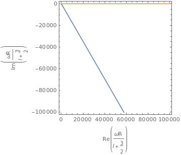
The Stokes graphs can be classified according to how the Stokes regions are adjacent to each other (or which triangulation of $\Sigma$ the Stokes graph is mapped). If we continuously change $\theta=\arg(\eta)$, the state of the adjacent of the Stokes regions may be discontinuously changed at specific values of $\arg(\eta)$. We refer the discontinuous change of the Stokes graph as saddle reduction [3]. We specify when this saddle reduction occurs with respect to the value of $\omega R/\left(l+\frac{3}{2}\right)$ instead of $\arg(\eta)$. The sign of the saddle reduction is to appear the Stokes line that connects two zeros of $Q_{0}(z)$. By definition of the Stokes lines (2.26), the parameters at which two of $z_{1},z_{2},z_{3}$ are connected can be determined by the following equations,

$$\Im\left[e^{i\theta}\int_{z_{1}}^{z_{3}}p_{0}\left(z\right)dz\right]=0,$$

(3.1)

$$\Im\left[e^{i\theta}\int_{z_{2}}^{z_{3}}p_{0}\left(z\right)dz\right]=0,$$

(3.2)

$$\Im\left[e^{i\theta}\int_{z_{1}}^{z_{2}}p_{0}\left(z\right)dz\right]=0.$$

(3.3)

The integrals in the square brackets are the elliptic integrals and can also be expressed by the hypergeometric function [18, 19],

$$\int_{z_{1}}^{z_{3}}p_{0}\left(z\right)dz=i\pi\left(l+\frac{3}{2}\right)\ _{2}F_{1}\left[-\frac{1}{6},\frac{1}{6},1,\frac{27\omega^{6}R^{6}}{4(l+\frac{3}{2})^{6}}\right],$$

(3.4)

$$\int_{z_{2}}^{z_{3}}p_{0}\left(z\right)dz=\left\{\begin{array}[]{l}-\frac{\pi\omega R\left(1-\frac{4(l+\frac{3}{2})^{6}}{27\omega^{6}R^{6}}\right)}{2\sqrt[3]{2}\sqrt{3}}\ _{2}F_{1}\left[\frac{5}{6},\frac{5}{6},2,1-\frac{4(l+\frac{3}{2})^{6}}{27\omega^{6}R^{6}}\right]\ \ \left(-\frac{\pi}{6}\leq\arg(\omega R)\leq 0\right),\\ \int_{z_{1}}^{z_{3}}p_{0}\left(z\right)dz-e^{i\frac{\pi}{3}}\frac{\pi\omega R\left(1-\frac{4(l+\frac{3}{2})^{6}}{27\omega^{6}R^{6}}\right)}{2\sqrt[3]{2}\sqrt{3}}\ _{2}F_{1}\left[\frac{5}{6},\frac{5}{6},2,1-\frac{4(l+\frac{3}{2})^{6}}{27\omega^{6}R^{6}}\right]\\ \ \ \ \ \ \ \ \ \ \ \ \ \ \ \ \ \ \ \ \ \ \ \ \ \ \ \ \ \ \ \ \ \ \ \ \ \ \ \ \ \ \ \ \ \ \ \ \ \ \ \ \ \ \ \ \left(-\frac{\pi}{2}\leq\arg(\omega R)<-\frac{\pi}{6}\right),\end{array}\right.$$

(3.5)

$$\int_{z_{1}}^{z_{2}}p_{0}\left(z\right)dz=-\int_{z_{2}}^{z_{3}}p_{0}\left(z\right)dz+\int_{z_{1}}^{z_{3}}p_{0}\left(z\right)dz.$$

(3.6)

These are local expressions but we can also compute each integral for other parameter regions by analytically continuing the hypergeometric function. By substituting (3.4)$\sim$(3.6) into (3.1)$\sim$(3.3), we can determine the values of the parameters occurring the saddle reduction. Fig.3.1 shows the values of $\omega R/\left(l+\frac{3}{2}\right)$ satisfying (3.1)$\sim$(3.3) at $\arg(\eta)=0$ in a range. Fig.3.1 indicates that the Stokes line connecting $z_{1}$ and $z_{2}$ appears at $\arg(\omega R)=-\frac{\pi}{3}$. Therefore the state of the adjacent of the Stokes regions is discontinuously changed between $-\frac{\pi}{3}<\arg(\omega R)<0$ and $-\frac{\pi}{2}\leq\arg(\omega R)<-\frac{\pi}{3}$.

Let us see examples of the Stokes graphs. Fig.3.2 shows the Stokes graph for $\arg(\eta)=0$ and $\omega R/\left(l+\frac{3}{2}\right)=\frac{2}{3}-i\frac{2}{30}$, which is in the region $-\frac{\pi}{3}<\arg(\omega R)<0$. For $\arg(\eta)=0$ and $-\frac{\pi}{3}<\arg(\omega R)<0$, the Stokes regions are adjacent each other in the same way as Fig.3.2 (for example, the Stokes region $\mathrm{I}_{\infty}$ is adjacent to $\mathrm{I}_{\mathrm{mid}}$, and $\mathrm{I}_{\mathrm{mid}}$ is adjacent to $\mathrm{I}_{0}$.).

Fig.3.3 shows the saddle reduction at $\arg(\omega R)=-\frac{\pi}{3}$ with $|\omega R/\left(l+\frac{3}{2}\right)|=|\frac{2}{3}-i\frac{2}{30}|$. In the graph $\mathrm{[a]}$, the state of the adjacent of the Stokes regions does not change from Fig.3.2 (the Stokes region $\mathrm{I}_{\infty}$ is adjacent to $\mathrm{I}_{\mathrm{mid}}$, and $\mathrm{I}_{\mathrm{mid}}$ is adjacent to $\mathrm{I}_{0}$). In the graph $\mathrm{[b]}$, two Stokes lines emanating from $z_{1}$ and $z_{2}$ overlap and become one Stokes line connecting $z_{1}$ and $z_{2}$. Continuing to decrease $\arg(\omega R)$, we obtain the graph $\mathrm{[c]}$ and $\mathrm{[d]}$. In these cases, the Stokes line connecting $z_{1}$ and $z_{2}$ in $\mathrm{[b]}$ separates again but their positions invert. The new Stokes region $\tilde{\mathrm{I}}_{\mathrm{mid}}$ then appears between $\mathrm{I}_{\mathrm{mid}}$ and $\mathrm{I}_{0}$. For $\arg(\eta)=0$ and $-\frac{\pi}{2}\leq\arg(\omega R)<-\frac{\pi}{3}$, the Stokes regions are adjacent each other in the same way as $\mathrm{[c]}$ and $\mathrm{[d]}$ in Fig.3.3.

We solve the connection problem of the Borel resummed WKB solutions for $\arg(\eta)=0$ from $z=\infty$ to the origin based on the Stokes graphs.

We impose the boundary conditions (i) only outgoing wave exists at $z\rightarrow+\infty$ and (ii) only ingoing wave exists at $z\rightarrow 0$ on the Borel resummed WKB solutions. The outgoing wave at $z\rightarrow+\infty$ is $\mathcal{B}\left[\psi_{z_{3},\mathrm{I_{\infty}}}^{+}\right](z)$. According to the connection formulae (3.11) and (3.16), $\mathcal{B}\left[\psi_{z_{3},\mathrm{I_{\infty}}}^{+}\right](z)$ is connected to the origin as follows,

$$\mathcal{B}\left[\psi_{z_{3},\mathrm{I_{\infty}}}^{+}\right](z)=\left\{\begin{array}[]{l}\left(1+e^{\eta\mathcal{B}\left[\Pi_{\gamma_{23}}\right]}\right)\mathcal{B}\left[\psi_{z_{3},\mathrm{I_{0}}}^{+}\right](z)-i\mathcal{B}\left[\psi_{z_{3},\mathrm{I_{0}}}^{-}\right](z)\ \ \left(-\frac{\pi}{3}<\arg(\omega R)<0\right),\\ \left(1+\left(1+e^{\eta\mathcal{B}\left[\Pi_{\gamma_{12}}\right]}\right)e^{\eta\mathcal{B}\left[\Pi_{\gamma_{23}}\right]}\right)\mathcal{B}\left[\psi_{z_{3},\mathrm{I_{0}}}^{+}\right](z)-i\mathcal{B}\left[\psi_{z_{3},\mathrm{I_{0}}}^{-}\right](z)\\ \ \ \ \ \ \ \ \ \ \ \ \ \ \ \ \ \ \ \ \ \ \ \ \ \ \ \ \ \ \ \ \ \ \ \ \ \ \ \ \ \ \ \ \ \ \ \ \ \ \ \ \ \ \ \ \ \ \ \ \left(-\frac{\pi}{2}\leq\arg(\omega R)<-\frac{\pi}{3}\right).\end{array}\right.$$

(3.17)

The ingoing wave at $z\rightarrow 0$ is $\mathcal{B}\left[\psi_{z_{3},\mathrm{I_{0}}}^{-}\right](z)$. Therefore to satisfy the boundary conditions, the coefficients of $\mathcal{B}\left[\psi_{z_{3},\mathrm{I_{0}}}^{+}\right](z)$ in (3.17) need to be zero,

$$\left\{\begin{array}[]{l}1+e^{\eta\mathcal{B}\left[\Pi_{\gamma_{23}}\right]}=0\ \ \ \ \ \ \ \ \ \ \ \ \ \ \ \ \ \ \ \ \ \ \left(-\frac{\pi}{3}<\arg(\omega R)<0\right),\\ 1+\left(1+e^{\eta\mathcal{B}\left[\Pi_{\gamma_{12}}\right]}\right)e^{\eta\mathcal{B}\left[\Pi_{\gamma_{23}}\right]}=0\ \ \left(-\frac{\pi}{2}\leq\arg(\omega R)<-\frac{\pi}{3}\right).\end{array}\right.$$

(3.18)

Taking the logarithm of (3.18) and substituting $\eta=1$, we obtain the following conditions,

$$\left\{\begin{array}[]{l}\mathcal{B}\left[\Pi_{\gamma_{23}}\right]=2\pi i\left(n+\frac{1}{2}\right)\ \ \ \ \ \ \ \ \ \ \ \ \ \ \ \ \ \ \ \ \ \ \ \ \ \ \ \ \left(-\frac{\pi}{3}<\arg(\omega R)<0\right),\\ \mathcal{B}\left[\Pi_{\gamma_{23}}\right]+\log\left(1+e^{\mathcal{B}\left[\Pi_{\gamma_{12}}\right]}\right)=2\pi i\left(n+\frac{1}{2}\right)\ \ \left(-\frac{\pi}{2}\leq\arg(\omega R)<-\frac{\pi}{3}\right),\end{array}\right.$$

(3.19)

where $n\in\mathbb{Z}_{\geq 0}$. The conditions (3.19) are satisfied by discrete sets of $\omega$, which are the quasi-normal modes for the massless scalar perturbation in the extremal M5-brane metric. Without considering convergence of the asymptotic series, the asymptotic expansion of (3.19) provides the following conditions,

$$\left\{\begin{array}[]{l}\Pi_{\gamma_{23}}=2\pi i\left(n+\frac{1}{2}\right)\ \ \ \ \ \ \ \ \ \ \ \ \ \ \ \ \ \ \ \ \ \ \ \ \left(-\frac{\pi}{3}<\arg(\omega R)<0\right),\\ \Pi_{\gamma_{23}}+\log\left(1+e^{\Pi_{\gamma_{12}}}\right)=2\pi i\left(n+\frac{1}{2}\right)\ \ \left(-\frac{\pi}{2}\leq\arg(\omega R)<-\frac{\pi}{3}\right).\end{array}\right.$$

(3.20)

The first condition of (3.20) is the all-order extension of the Bohr-Sommerfeld condition (2.7).

References

• [1] A. Voros, Ann. I.H.P. 39, 211 (1983).
• [2] E. Delabaere and F. Pham, Annales de l’IHP 71, 1-94 (1999).
• [3] K. Iwaki and T. Nakanishi, J. Phys. A: Math. Theor. 47 (2014), 474009 [arXiv:1401.7094 [math.CA]].
• [4] E. Delabaere, H. Dillinger and F. Pham, J.Math.Phys. 38, 6126 (1997).
• [5] K. Ito, M. Mariño and H. Shu, JHEP 01 (2019), 228 [arXiv:1811.04812 [hep-th]].
• [6] N. Sueishi, S. Kamata, T. Misumi and M. Ünsal, JHEP 12 (2020), 114 [arXiv:2008.00379 [hep-th]].
• [7] Y. Emery, JHEP 07 (2021), 171 [arXiv:2008.13680 [hep-th]].
• [8] K. Imaizumi, Phys. Lett. B 834 (2022), 137450 [arXiv:2207.09961 [hep-th]].
• [9] E. W. Leaver, Proc. Roy. Soc. Lond. A 402, 285-298 (1985).
• [10] B. F. Schutz and C. M. Will, Astrophys. J Lett. 291 L33-36 (1985).
• [11] G. Aminov, A. Grassi and Y. Hatsuda, Annales Henri Poincare 23 (2022) no.6, 1951-1977 [arXiv:2006.06111 [hep-th]].
• [12] K. Ito, S. Kanno and T. Okubo, JHEP 08 (2017), 065 [arXiv:1705.09120 [hep-th]].
• [13] M. Bianchi, D. Consoli, A. Grillo and J. F. Morales, Phys. Lett. B 824 (2022), 136837 [arXiv:2105.04245 [hep-th]].
• [14] M. Bianchi, D. Consoli, A. Grillo and J. F. Morales, JHEP 01 (2022), 024 [arXiv:2109.09804 [hep-th]].
• [15] I. R. Klebanov, Nucl. Phys. B 496 (1997), 231-242 [arXiv:hep-th/9702076 [hep-th]].
• [16] R. Güven, Phys. Lett. B 276, 49-55 (1992).
• [17] D. Gaiotto, G. W. Moore and A. Neitzke, Adv. Math. 234 (2013), 239-403 [arXiv:0907.3987 [hep-th]].
• [18] A. Bilal and F. Ferrari, Nucl. Phys. B 480 (1996), 589-622 [arXiv:hep-th/9605101 [hep-th]].
• [19] D. Fioravanti, D. Gregori and H. Shu, [arXiv:2208.14031 [hep-th]].
• [20] J. Zinn-Justin and U. D. Jentschura, Annals Phys. 313 (2004), 197-267 [arXiv:quant-ph/0501136 [quant-ph]].
• [21] J. Zinn-Justin and U. D. Jentschura, Annals Phys. 313 (2004), 269-325 [arXiv:quant-ph/0501137 [quant-ph]].
• [22] G. Başar and G. V. Dunne, JHEP 02 (2015), 160 [arXiv:1501.05671 [hep-th]].
• [23] N. Sueishi, S. Kamata, T. Misumi and M. Ünsal, JHEP 07 (2021), 096 [arXiv:2103.06586 [quant-ph]].
• [24] E. W. Leaver, Phys. Rev. D 41, 2986–2997 (1990).
• [25] S. Prem Kumar, A. O’Bannon, A. Pribytok and R. Rodgers, JHEP 05 (2021), 109 [arXiv:2011.13859 [hep-th]].
• [26] L. Motl and A. Neitzke, Adv. Theor. Math. Phys. 7, 307-330 (2003) [gr-qc/0301173].
• [27] L. Motl, Adv. Theor. Math. Phys. 6 (2003), 1135-1162 [arXiv:gr-qc/0212096 [gr-qc]].
• [28] N. Andersson and C. J. Howls, Class. Quant. Grav. 21 (2004), 1623-1642 [arXiv:gr-qc/0307020 [gr-qc]].
• [29] A. Grassi, Q. Hao and A. Neitzke, JHEP 01 (2022), 046 [arXiv:2105.03777 [hep-th]].
• [30] D. Fioravanti and D. Gregori, [arXiv:2112.11434 [hep-th]].
• [31] G. Bonelli, C. Iossa, D. P. Lichtig and A. Tanzini, Phys. Rev. D 105 (2022) no.4, 044047 [arXiv:2105.04483 [hep-th]].
• [32] G. Bonelli, C. Iossa, D. P. Lichtig and A. Tanzini, [arXiv:2201.04491 [hep-th]].
• [33] D. Consoli, F. Fucito, J. F. Morales and R. Poghossian, [arXiv:2206.09437 [hep-th]].