Non-equispaced Fourier Neural Solvers for PDEs

Let $D\in\mathbb{R}^{d}$ be the bounded and open spatial domain where $n_{s}$-point discretization of the domain $D$ written as $\bm{X}=\{\bm{x}_{i}=(x_{i}^{(1)},\ldots,x_{i}^{(d)}):1\leq i\leq n_{s}\}$ are sampled. The observation of input function $a\in\mathcal{A}(D;\mathbb{R}^{d_{a}})$ and output $u\in\mathcal{U}(D;\mathbb{R}^{d_{u}})$ on the $n_{s}$ points are denoted by $\{a(\bm{x}_{i}),u(\bm{x}_{i})\}_{i=1}^{n_{s}}$, where $\mathcal{A}(D;\mathbb{R}^{d_{a}})$ and $\mathcal{U}(D;\mathbb{R}^{d_{u}})$ are separable Banach spaces of function taking values in $\mathbb{R}^{d_{a}}$ and $\mathbb{R}^{d_{u}}$ respectively. Suppose $\bm{x}\sim\mu$ is i.i.d. sampled from the probability measure $\mu$ supported on $D$. An infinite-dimensional neural operator $\mathcal{G}_{\theta}:\mathcal{A}(D;\mathbb{R}^{d_{a}})\rightarrow\mathcal{U}(D;\mathbb{R}^{d_{u}})$ parameterized by $\theta\in\Theta$, aims to build an approximation so that $\mathcal{G}_{\theta}(a)\approx u$. A cost functional $\mathcal{C}:\mathcal{U}(D;\mathbb{R}^{d_{u}})\times\mathcal{U}(D;\mathbb{R}^{d_{u}})\rightarrow\mathbb{R}$ is defined to optimize the parameter $\theta$ of the operator by the objective

To establish a mesh-invariant operator, $\bm{X}$ can be non-equispaced, and the learned $\mathcal{G}_{\theta}$ should be transferred to an arbitary discretization $\bm{X}^{\prime}\in D$, where $\bm{x}\in\bm{X^{\prime}}$ can be not necessarily contained in $\bm{X}$. Because we focus on spatially non-equispaced points, when the PDE system is time-dependent, we assume that timestamps $\{t_{j}\}$ are uniformly sampled, which means we do not focus on temporally irregular sampling or continuous time problem (Rubanova et al. 2019; Chen et al. 2019; Çağatay Yıldız et al. 2019; Iakovlev et al. 2020).

Let $\bm{k}_{l}=(k_{l}^{(1)},\ldots,k_{l}^{(d)})$ the $l$-th frequency corresponding to $\bm{X}$, with $\bm{k}_{l}\in\mathbb{Z}^{d}$. The discrete Fourier transform of $f:D\rightarrow\mathbb{R}^{d_{f}}$ is denoted by $\mathcal{F}(f)(\bm{k})\in\mathbb{C}^{d_{f}}$, with $\mathcal{F}^{-1}$ as its inverse, then

where $j$ means the $j$-th dimension of $f$. General Fourier transforms have complexity $O(n_{s}^{2})$. When the spatial points are distributed uniformly on equispaced grids, fast Fourier transform (FFT) and its inverse (IFFT) (Rader & Brenner 1976) can be implemented to reduce the complexity to $O(n_{s}\log n_{s})$.

Neural Operators. To model one specific instance of PDEs, a line of neural solvers have been designed, with prior physical knowledge as constraints. Different from these methods, neural operators (Lu et al. 2021; Nelsen & Stuart 2021) require no knowledge of underlying PDEs, and only data. Finite-dimensional operator methods (Guo et al. 2016; Sirignano & Spiliopoulos 2018; Bhatnagar et al. 2019; KHOO et al. 2020) are discretization-variant, meaning that the model can only learn the patterns of the spatial points which have been fed to the model in the training process. By contrast, infinite-dimensional operator methods (Li et al. 2020b; Li et al. 2020c; Bhattacharya et al. 2021; Brandstetter et al. 2022) are proposed to be discretization-invariant, enabling the learned models to generalize well to unseen meshes with zero-shot.

Kernel integral operator method (Li et al. 2020a) is a family of infinite-dimensional operators, in which $(\mathcal{G}_{\theta}(a))(\bm{x})=Q\circ v^{\rm{T}}\circ\cdots\circ v^{\rm{1}}\circ P(a)(\bm{x})$ is formulated as an iterative architecture. A higher-dimensional representation function is first obtained by $v^{\rm{0}}=P(a)\in\mathcal{U}(D;\mathbb{R}^{d_{v}})$, where $P$ is a shallow fully-connected network. It is updated by

where $\mathcal{K}_{\phi}:\mathcal{A}\rightarrow\mathcal{L}(\mathcal{U})$ is a kernel integral operator mapping, mapping $a$ to bounded linear operators, with parameters $\phi$. $W$ is a linear transform and $\sigma$ is a non-linear activation function. After the final iteration, $Q$ projects $v^{\mathrm{T}}(\bm{x})$ back to $\mathcal{U}(D;\mathbb{R}^{d_{u}})$.

Fourier Neural Operator (FNO) (Li et al. 2020c) as a member in kernel integral operator methods, updates the representation by applying the convolution theorem as:

where $R_{\phi}$ as the Fourier transform of a periodic kernel function $\kappa_{\phi}$, is directly learned as the parameters in the updating process. To be resolution-invariant, FNO picks a finite-dimensional parameterization by truncating the Fourier series of both $\mathcal{F}(v)$ and $R_{\phi}$ as a maximal number of modes $k^{(l)}_{\rm{max}}$ for $1\leq l\leq d$. Because the sampled spatial points are equispaced in FNO, it can conduct FFT and IFFT to get the Fourier series, which can be very efficient.

Vision Mixers (Tolstikhin et al. 2021; Rao et al. 2021; Guibas et al. 2021) are a line of models with a stack of (token mixing) - (channel mixing) - (token mixing) as their network structure for vision tasks. They are based on the assumption that the key component for the effectiveness of Vision Transformers (ViT) (Dosovitskiy et al. 2020) is attributed to the proper mixing of tokens. The defined tokens are equivalent to equispaced spatial points in the former definition, and the research on the mixing of them can be an analogy to modeling the proper interaction or message-passing patterns among spatial points. In specific, ViT uses a non-Mercer kernel function (Wright & Gonzalez 2021) $\kappa_{\phi}$ to adaptively learn the pattern of message-passing through the iterative updating process

where $W$ is a linear transform called channel mixing layer because it transforms the input on the channel of an image whose dimension is equivalent to function dimension $d_{f}$. Note that we omit the residual connection in Eq. (3) for simplicity.

Remark. The FNO can be regarded as a member of the family of Vision Mixers. The reason is that a component in an iteration in Eq. (4) can be written as $(R_{\phi}\cdot\mathcal{F}(v))(\bm{x})=R_{\phi}\cdot\sum_{i}e^{-2\pi i<\bm{x},\bm{x}_{i}>}v(\bm{x}_{i})$, because in the equispaced scenarios, $\bm{x}_{i}$ can be regarded as lying on the same grids as $\bm{k}$ after scaling. The kernel $\kappa_{\phi}$ is parameterized by $\kappa_{\phi}(\bm{x},\bm{x}_{i},v(\bm{x}),v(\bm{x}_{i}))=e^{-2\pi i<\bm{x},\bm{x}_{i}>}$ , and the matrix multiplication of $R_{\phi}$ also performs mixing on channels. Besides, the inverse Fourier transform can also be regarded as token mixing layers, or so-called token demixing layers (Guibas et al. 2021).

However, the powerful fitting ability and efficiency of Vision Mixers are limited to being applied to non-equispaced spatial points. Another option for non-equispaced data is graph spatio-temporal models, in which interaction patterns among spatial points are modeled in a graph message-passing way (Gilmer et al. 2017; Atwood & Towsley 2016; Defferrard et al. 2017). The mechanism is similar to the token mixing in Vision Mixers by means of the summation in Eq. (5) conducted in the predefined neighborhood of each point. Unfortunately, the graph spatio-temporal models (Seo et al. 2016; Li et al. 2018; Bai et al. 2020; Lin et al. 2021) suffer from high computational complexity and unsatisfactory accuracy in solving complex dynamical systems (such as turbulent flows).

Since FNO belongs to Vision Mixers, this firstly raised a question to us: Do models employing Vision Mixers’s architecture have the potential to model complex PDE systems? Thus, experiments are conducted to give an intuitive explanation of our motivation as shown in Fig. 2. The data are generated by Navier-Stokes equations. It is noted that graph spatio-temporal methods can also handle the equispaced data. Detailed setup is given in Sec. 4.

We find that (1) All of the evaluated Vision Mixers are able to model the dynamical systems effectively, in spite of FNO as the only discretization-invariant model; (2) The complex dynamics of the systems are hardly captured by graph spatio-temporal models, whose performance on both accuracy and computational efficiency is very unsatisfactory in either equispaced or non-equispaced scenarios. Fig. 2(c) shows the problem of infeasibility of graph spatio-temporal models through the loss curves on the validation set, compared with Vision Mixers. However, Vision Mixers fail to handle the non-equispaced data. Therefore, we aim to (1) establish a mesh-invariant model, by harnessing the network structure of Vision Mixers to achieve competitive efficiency and effectiveness in equispaced scenarios, as shown in Fig. 2(a); (2) Besides, it should allow applicability and comparable accuracy in non-equispaced scenarios for solving PDEs, as shown in Fig. 2(b).

Nonuniformly signals are unavoidable in certain real-world physics scenarios, such as signals obtained by meteorological stations on the earth surface, which urge the fast Fourier transform (FFT) to be extended to non-equispaced data with efficient implementation of FFT. Non-equispaced FFTs usually rely on a mixture of interpolation and the judicious use of FFT, where the calculations of interpolation are no more than $O(n_{s}\log n_{s})$ operations (Kalamkar et al. 2012; Cheema et al. 2017). For example, Lagrange interpolation is used to approximate the signal values on $m_{s}$ resampled equispaced points $\{\bm{x}_{j}\}_{1\leq j\leq m_{s}}$, and then implement FFT on the interpolated points. A low rank approximation with complexity of $O(n_{s}\log(1/\epsilon))$ is used to replace the interpolation with complexity of $O(n_{s}^{2})$ with $\epsilon$ as the precision of computations (Dutt & Rokhlin 1995). Another example is commonly used Gaussian-based interpolation (Kestur et al. 2010). Denote $\mathcal{F}$ as equispaced FFT in particular, and $\mathcal{H}$ as the interpolation operator, and the proposed non-equispaced FFT can be written as

$\mathcal{H}(f)(\bm{x}_{j})=\sum_{i=1}^{n_{s}}f(\bm{x}_{i})h_{\tau}(\bm{x}_{i}-\bm{x}_{j})$ interpolates values on resampled points via convolution with the periodic heat kernel $h_{\tau}(\bm{x}-\bm{y})=\sum_{\bm{l}\in\mathbb{Z}^{d}}e^{-(\bm{x}-\bm{l})^{2}/4\tau}$, with $\tau$ as a constant. Multiplication of the inperploation matrix $(H_{\tau})_{i,j}=h_{\tau}(\bm{x}_{i}-\bm{x}_{j})$ and the signal vector $(\bm{f})_{i}=f(\bm{x}_{i})$ includes $O(n_{s}m_{s})\approx O(n_{s}^{2})$ operations. For the kernel $h_{\tau}$, it is a summation of Gaussian kernel, and convolution with a single Gaussian in each points $\bm{x}_{i}$’s neighborhood $\mathcal{N}(\bm{x}_{i})$ can yeid a tiny error depending on $\tau$, so the interpolation operator can be approximate via $\mathcal{H}(f)(\bm{x}_{j})=\sum_{\bm{x}_{j}\in\mathcal{N}(\bm{x}_{i})}f(\bm{x}_{i})h_{\tau}(\bm{x}_{i}-\bm{x}_{j})$. Restricting the neighbor number to $|\mathcal{N}(\bm{x}_{i})|\leq\log n_{s}$ leads the complexity to reduce to $O(n_{s}\log n_{s})$.

Benchmarks for comparison. For finite-dimensional operators, we choose Vision Mixers including ViT (Dosovitskiy et al. 2020), GFN (Rao et al. 2021) and MLPMixer (Tolstikhin et al. 2021) as equispaced problem solvers, with DeepONet-V and DeepONet-U as two variants for DeepONet(Lu et al. 2021) and graph spatio-temporal models including DCRNN (Li et al. 2018), AGCRN (Bai et al. 2020) and GCGRU (Seo et al. 2016) as non-equispaced problem solvers. For infinite-dimensional operators, the state-of-the-art FNO (Li et al. 2020c) for equispaced problems and MPPDE (Brandstetter et al. 2022) for non-equispaced problems are chosen. A brief introduction to these models is shown in Appendix. B.1. In Vision Mixers, the different timestamps in temporal axis are also regarded as ‘tokens’ in that timestamps are uniformly sampled.

Protocol. The widely-used metrics - Mean Absolute Error (MAE) and Root Mean Square Error (RMSE) are deployed to measure the performance. The reported mean and standard deviation of metrics are obtained through 5 independent experiments. All the models for comparison are trained with target function of MSE, i.e. $\mathcal{C}(u,v)(\bm{x})=||u(\bm{x})-v(\bm{x})||^{2}$ corresponding to Eq. (1), and optimized by Adam optimizer in 500 epochs. The hyper-parameters are chosen through a carefully tuning on the validation set. Every trial is implemented on a single Nvidia-V100 (32510MB).

Data. We choose four equations for numerical experiments, three of which are time-dependent (KdV, Burgers’ and NS), while the other one is not (Darcy Flows). For 1-d problem, we consider Korteweg de Vries (KdV) and Burgers’ equation (given in Appendix. B.2.).

For 2-d PDEs, we consider Darcy Flow (given in Appendix. B.2.) and Navier-Stokes (NS) equation for a viscous, incompressible fluid in vorticity form on the unit torus:

where $\bm{x}\in[0,1]^{2},t\in[0,1]$. $u$ is the velocity field, $w=\nabla\times u$ is the vorticity, $w_{0}$ is the initial vorticity, $\nu\in\mathbb{R}^{+}$ is the viscosity coefficient, and $f$ is the forcing function.

The total number of instances is 1200, with percentages of 0.7, 0.1 and 0.2 for training, validating and testing, respectively. The original simulated resolutions of PDE signals are $128\times 128$ in NS equation. For others, see Appendix. B.2. When evaluating their performance in equispaced scenarios of different resolutions, we can downsample the resolution for training to low-resolution data, e.g. $64\times 64$ in NS equation. To evaluate their performance in non-equispaced scenarios of different meshes, we randomly choose $n_{s}$ spatial points for training.

Performance comparison. In this part, for time-dependent PDEs, our target is to map the observed physical quantities from initial condition $u(\bm{X},\bm{T})\in\mathbb{R}^{n_{s}\times n_{t}}$, where $\bm{T}=\{t_{i}:t_{i}<T\}_{1\leq i\leq n_{t}}$, to quantities at some later time $u(\bm{X},\bm{T^{\prime}})\in\mathbb{R}^{n_{s}\times n^{\prime}_{t}}$, where $\bm{T^{\prime}}=\{t_{i}:T<t_{i}<T^{\prime}\}_{1\leq i\leq n^{\prime}_{t}}$. We set the input timestamp number $n_{t}$ as 1 (initial state to future dynamics) and 10 (sequence to sequence), and prediction horizon $n^{\prime}_{t}$ as 10, 20 and 40 as short-, mid- and long-term settings. For Darcy Flows, which are independent of time, we directly build an operator to map $a$ to $u$. In equispaced scenarios, the resolution is denoted by $r^{d}=n_{s}$, where $d$ is the spatial dimension. In non-equispaced scenarios, the spatial points number is denoted by $n_{s}$. The comparison of benchmarks with or without equispace-unnecessity are shown in Table. 1 and 2 respectively, and detailed results including KdV equations with RMSE and standard deviations are given in Appendix. B.3. It can be concluded that (1) In equispaced scenarios, the proposed NFS obtains the lowest error in most 1-d PDE settings, and in solving 2-d PDEs, its superiority over other Vision Mixers are significant, with $42.85\%$ improvements on MAE according to the trials of NS ($r=64,n_{t}=10,n^{\prime}_{t}=40$). (2) In non-equispaced scenarios, the evaluated graph spatio-temporal models’ performance is unsatisfactory, especially in NS equations. In comparison, NFS achieves comparable high accuracy to the equispaced scenarios, for instance, according to columns of NS ($r=64,n_{t}=10,n^{\prime}_{t}=40$) with ($n_{s}=4096,n_{t}=10,n^{\prime}_{t}=40$). (3) In some trials such as Burgers’ ($n_{t}=1$) in Table. B4 in Appendix. B.3, Vison Mixers including FNO also suffer from non-convergence of loss; while NFS can still generate accurate predictions. The explanation of the phenomenon will be our future work.

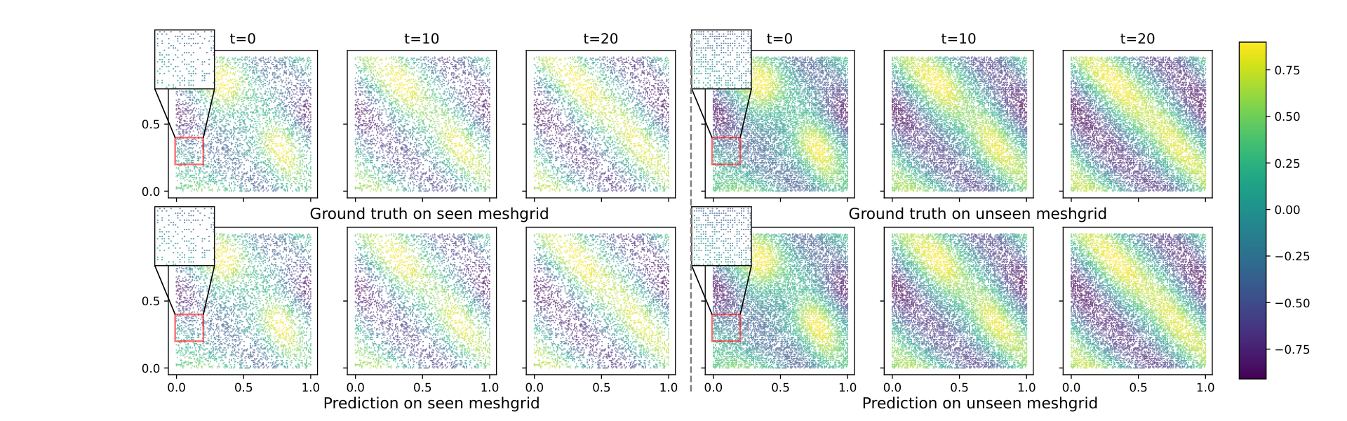
Mesh-invariance evaluation. We use $(u(\bm{X},\bm{T}),u(\bm{X},\bm{T^{\prime}}))$ as the training set, and evaluate the model’s performance of mesh-invariant inference ability on $\bm{X^{\prime}}$, where $|\bm{X^{\prime}}|=n^{\prime}_{s}$. $\bm{X^{\prime}}$ is a different mesh with $\bm{X}\subseteq\bm{X^{\prime}}$. The visualization results of NS ($n_{s}=4096,n^{\prime}_{t}=40$) are shown in Fig. 4. For a fixed $n^{\prime}_{s}$, we randomly sampled different $\bm{X^{\prime}}$ for 100 times, to get the mean errors and standard deviations (given in Appendix. B.5) of different spatial meshes. We can conclude from Table. 3 that (1) The errors on unseen meshes are larger than the errors on seen meshes, showing the overfitting effects. However, the errors on unseen meshes are acceptable, since they are even lower than other models’ prediction error on seen meshes. (2) Larger $n^{\prime}_{s}$ leads to higher prediction error because a large number of unseen points are likely to disturb the learned token mixing patterns. On the other hand, NS ($n_{s}=1024,n^{\prime}_{t}=10$) implies that small spatial point numbers of training meshes ($n_{s}$) hinder model’s generalizing ability on unseen meshes, due to excessive loss of spatial information.

Two modules in NFS differ from FNO. The first is the interpolation layers at the beginning and the end of the architecture. The second is the extra Layer-Norm in the FNO layers, which can be applicable in NFS thanks to its fixed resampled equispaced points, but inapplicable to FNO for preserving its resolution-invariance. We aim to figure out what makes NFS outperform FNO.

Since NFS can be regarded as a combination of our interpolation layers with the revised FNO, our interpolation layers can also be implemented in the other Vision Mixers, so that these methods are equipped with the ability to handle non-equispaced data. Details are given in Appendix. B.7. We find that (1) From Table. B10 and Table. 1, the degeneration of performance is obvious in other Vision Mixers. In comparison, FNO as intermediate equispaced layers, truncates the high frequency in its channel mixing and retains the low frequency shared by both resampled and original signals, so the loss of accuracy in non-equispaced scenarios is tiny in our NFS; (2) Although the performance on unseen meshes is more stable in these non-equispaced Vision Mixers, the performance gap is still large, according to Table. B10 and Table. 3.

The discussed Fig. 2 shows time complexity of each method. Vision Mixers are the fastest, while graph spatio-temporal models are far much slower. NFS falls in between because the interpolation layer can be an analogy to a graph-message-passing layer (See Sec. 3.3), and the intermediate are equispaced token-channel mixing layers of Vision Mixers’ structure. Memory usage shows storing each point’s neighbors in the interpolation layer is very memory-consuming.

References

- Atwood & Towsley (2016) James Atwood and Don Towsley. Diffusion-convolutional neural networks, 2016.
- Ba et al. (2016) Jimmy Lei Ba, Jamie Ryan Kiros, and Geoffrey E. Hinton. Layer normalization, 2016. URL https://arxiv.org/abs/1607.06450.
- Bai et al. (2020) Lei Bai, Lina Yao, Can Li, Xianzhi Wang, and Can Wang. Adaptive graph convolutional recurrent network for traffic forecasting, 2020.
- Bar & Sochen (2019) Leah Bar and Nir Sochen. Unsupervised deep learning algorithm for pde-based forward and inverse problems, 2019.
- Bhatnagar et al. (2019) Saakaar Bhatnagar, Yaser Afshar, Shaowu Pan, Karthik Duraisamy, and Shailendra Kaushik. Prediction of aerodynamic flow fields using convolutional neural networks. Computational Mechanics, 64(2):525–545, jun 2019. doi: 10.1007/s00466-019-01740-0. URL https://doi.org/10.1007%2Fs00466-019-01740-0.
- Bhattacharya et al. (2021) Kaushik Bhattacharya, Bamdad Hosseini, Nikola B. Kovachki, and Andrew M. Stuart. Model reduction and neural networks for parametric pdes, 2021.
- Brandstetter et al. (2022) Johannes Brandstetter, Daniel Worrall, and Max Welling. Message passing neural pde solvers, 2022. URL https://arxiv.org/abs/2202.03376.
- Cheema et al. (2017) Umer I. Cheema, Gregory Nash, Rashid Ansari, and Ashfaq Khokhar. Memory-optimized re-gridding architecture for non-uniform fast fourier transform. IEEE Transactions on Circuits and Systems I: Regular Papers, 64(7):1853–1864, 2017. doi: 10.1109/TCSI.2017.2681723.
- Chen et al. (2019) Ricky T. Q. Chen, Yulia Rubanova, Jesse Bettencourt, and David Duvenaud. Neural ordinary differential equations, 2019.
- Chen & Chen (1995) Tianping Chen and Hong Chen. Universal approximation to nonlinear operators by neural networks with arbitrary activation functions and its application to dynamical systems. IEEE Transactions on Neural Networks, 6(4):911–917, 1995. doi: 10.1109/72.392253.
- Chu et al. (2021) Xiangxiang Chu, Zhi Tian, Yuqing Wang, Bo Zhang, Haibing Ren, Xiaolin Wei, Huaxia Xia, and Chunhua Shen. Twins: Revisiting the design of spatial attention in vision transformers, 2021. URL https://arxiv.org/abs/2104.13840.
- Defferrard et al. (2017) Michaël Defferrard, Xavier Bresson, and Pierre Vandergheynst. Convolutional neural networks on graphs with fast localized spectral filtering, 2017.
- Dong et al. (2021) Yihe Dong, Jean-Baptiste Cordonnier, and Andreas Loukas. Attention is not all you need: Pure attention loses rank doubly exponentially with depth, 2021. URL https://arxiv.org/abs/2103.03404.
- Dosovitskiy et al. (2020) Alexey Dosovitskiy, Lucas Beyer, Alexander Kolesnikov, Dirk Weissenborn, Xiaohua Zhai, Thomas Unterthiner, Mostafa Dehghani, Matthias Minderer, Georg Heigold, Sylvain Gelly, Jakob Uszkoreit, and Neil Houlsby. An image is worth 16x16 words: Transformers for image recognition at scale, 2020. URL https://arxiv.org/abs/2010.11929.
- Dutt & Rokhlin (1995) A. Dutt and V. Rokhlin. Fast fourier transforms for nonequispaced data, ii. Applied and Computational Harmonic Analysis, 2(1):85–100, 1995. ISSN 1063-5203. doi: https://doi.org/10.1006/acha.1995.1007. URL https://www.sciencedirect.com/science/article/pii/S106352038571007X.
- E & Yu (2017) Weinan E and Bing Yu. The deep ritz method: A deep learning-based numerical algorithm for solving variational problems, 2017.
- Gilmer et al. (2017) Justin Gilmer, Samuel S. Schoenholz, Patrick F. Riley, Oriol Vinyals, and George E. Dahl. Neural message passing for quantum chemistry, 2017.
- Guibas et al. (2021) John Guibas, Morteza Mardani, Zongyi Li, Andrew Tao, Anima Anandkumar, and Bryan Catanzaro. Adaptive fourier neural operators: Efficient token mixers for transformers, 2021. URL https://arxiv.org/abs/2111.13587.
- Guo et al. (2016) Xiaoxiao Guo, Wei Li, and Francesco Iorio. Convolutional neural networks for steady flow approximation. In Proceedings of the 22nd ACM SIGKDD International Conference on Knowledge Discovery and Data Mining, KDD ’16, pp. 481–490, New York, NY, USA, 2016. Association for Computing Machinery. ISBN 9781450342322. doi: 10.1145/2939672.2939738. URL https://doi.org/10.1145/2939672.2939738.
- Hornik et al. (1989) Kurt Hornik, Maxwell Stinchcombe, and Halbert White. Multilayer feedforward networks are universal approximators. Neural Networks, 2(5):359–366, 1989. ISSN 0893-6080. doi: https://doi.org/10.1016/0893-6080(89)90020-8. URL https://www.sciencedirect.com/science/article/pii/0893608089900208.
- Iakovlev et al. (2020) Valerii Iakovlev, Markus Heinonen, and Harri Lähdesmäki. Learning continuous-time pdes from sparse data with graph neural networks, 2020. URL https://arxiv.org/abs/2006.08956.
- Kalamkar et al. (2012) Dhiraj D. Kalamkar, Joshua D. Trzaskoz, Srinivas Sridharan, Mikhail Smelyanskiy, Daehyun Kim, Armando Manduca, Yunhong Shu, Matt A. Bernstein, Bharat Kaul, and Pradeep Dubey. High performance non-uniform fft on modern x86-based multi-core systems. In 2012 IEEE 26th International Parallel and Distributed Processing Symposium, pp. 449–460, 2012. doi: 10.1109/IPDPS.2012.49.
- Kestur et al. (2010) Srinidhi Kestur, Sungho Park, Kevin M. Irick, and Vijaykrishnan Narayanan. Accelerating the nonuniform fast fourier transform using fpgas. In 2010 18th IEEE Annual International Symposium on Field-Programmable Custom Computing Machines, pp. 19–26, 2010. doi: 10.1109/FCCM.2010.13.
- KHOO et al. (2020) YUEHAW KHOO, JIANFENG LU, and LEXING YING. Solving parametric PDE problems with artificial neural networks. European Journal of Applied Mathematics, 32(3):421–435, jul 2020. doi: 10.1017/s0956792520000182. URL https://doi.org/10.1017%2Fs0956792520000182.
- Kovachki et al. (2021) Nikola Kovachki, Zongyi Li, Burigede Liu, Kamyar Azizzadenesheli, Kaushik Bhattacharya, Andrew Stuart, and Anima Anandkumar. Neural operator: Learning maps between function spaces, 2021. URL http://tensorlab.cms.caltech.edu/users/anima/pubs/GraphPDE_Journal.pdf.
- Li et al. (2018) Yaguang Li, Rose Yu, Cyrus Shahabi, and Yan Liu. Diffusion convolutional recurrent neural network: Data-driven traffic forecasting, 2018.
- Li et al. (2020a) Zongyi Li, Nikola Kovachki, Kamyar Azizzadenesheli, Burigede Liu, Kaushik Bhattacharya, Andrew Stuart, and Anima Anandkumar. Neural operator: Graph kernel network for partial differential equations, 2020a. URL https://arxiv.org/abs/2003.03485.
- Li et al. (2020b) Zongyi Li, Nikola Kovachki, Kamyar Azizzadenesheli, Burigede Liu, Kaushik Bhattacharya, Andrew Stuart, and Anima Anandkumar. Multipole graph neural operator for parametric partial differential equations, 2020b.
- Li et al. (2020c) Zongyi Li, Nikola Kovachki, Kamyar Azizzadenesheli, Burigede Liu, Kaushik Bhattacharya, Andrew Stuart, and Anima Anandkumar. Fourier neural operator for parametric partial differential equations, 2020c. URL https://arxiv.org/abs/2010.08895.
- Lin et al. (2021) Haitao Lin, Zhangyang Gao, Yongjie Xu, Lirong Wu, Ling Li, and Stan. Z. Li. Conditional local convolution for spatio-temporal meteorological forecasting, 2021.
- Lin et al. (2022) Haitao Lin, Guojiang Zhao, Lirong Wu, and Stan Z. Li. Stonet: A neural-operator-driven spatio-temporal network, 2022. URL https://arxiv.org/abs/2204.08414.
- Liu et al. (2021) Ze Liu, Yutong Lin, Yue Cao, Han Hu, Yixuan Wei, Zheng Zhang, Stephen Lin, and Baining Guo. Swin transformer: Hierarchical vision transformer using shifted windows, 2021. URL https://arxiv.org/abs/2103.14030.
- Lu et al. (2021) Lu Lu, Pengzhan Jin, Guofei Pang, Zhongqiang Zhang, and George Em Karniadakis. Learning nonlinear operators via deeponet based on the universal approximation theorem of operators. Nature Machine Intelligence, 3:218–229, 2021.
- Mao et al. (2021) Xiaofeng Mao, Gege Qi, Yuefeng Chen, Xiaodan Li, Ranjie Duan, Shaokai Ye, Yuan He, and Hui Xue. Towards robust vision transformer, 2021. URL https://arxiv.org/abs/2105.07926.
- Naseer et al. (2021) Muzammal Naseer, Kanchana Ranasinghe, Salman Khan, Munawar Hayat, Fahad Shahbaz Khan, and Ming-Hsuan Yang. Intriguing properties of vision transformers, 2021. URL https://arxiv.org/abs/2105.10497.
- Nelsen & Stuart (2021) Nicholas H. Nelsen and Andrew M. Stuart. The random feature model for input-output maps between banach spaces, 2021.
- Pan & Duraisamy (2020) Shaowu Pan and Karthik Duraisamy. Physics-informed probabilistic learning of linear embeddings of nonlinear dynamics with guaranteed stability. SIAM Journal on Applied Dynamical Systems, 19(1):480–509, Jan 2020. ISSN 1536-0040. doi: 10.1137/19m1267246. URL http://dx.doi.org/10.1137/19M1267246.
- Park & Kim (2022) Namuk Park and Songkuk Kim. How do vision transformers work?, 2022. URL https://arxiv.org/abs/2202.06709.
- Rader & Brenner (1976) C. Rader and N. Brenner. A new principle for fast fourier transformation. IEEE Transactions on Acoustics, Speech, and Signal Processing, 24(3):264–266, 1976. doi: 10.1109/TASSP.1976.1162805.
- Raissi et al. (2020) Maziar Raissi, Alireza Yazdani, and George Em Karniadakis. Hidden fluid mechanics: Learning velocity and pressure fields from flow visualizations. Science, 367(6481):1026–1030, 2020.
- Rao et al. (2021) Yongming Rao, Wenliang Zhao, Zheng Zhu, Jiwen Lu, and Jie Zhou. Global filter networks for image classification, 2021. URL https://arxiv.org/abs/2107.00645.
- Rubanova et al. (2019) Yulia Rubanova, Ricky T. Q. Chen, and David Duvenaud. Latent odes for irregularly-sampled time series, 2019.
- Seo et al. (2016) Youngjoo Seo, Michaël Defferrard, Pierre Vandergheynst, and Xavier Bresson. Structured sequence modeling with graph convolutional recurrent networks, 2016.
- Sirignano & Spiliopoulos (2018) Justin Sirignano and Konstantinos Spiliopoulos. DGM: A deep learning algorithm for solving partial differential equations. Journal of Computational Physics, 375:1339–1364, dec 2018. doi: 10.1016/j.jcp.2018.08.029. URL https://doi.org/10.1016%2Fj.jcp.2018.08.029.
- Smith et al. (2020) Jonathan D. Smith, Kamyar Azizzadenesheli, and Zachary E. Ross. Eikonet: Solving the eikonal equation with deep neural networks, 2020.
- Tolstikhin et al. (2021) Ilya Tolstikhin, Neil Houlsby, Alexander Kolesnikov, Lucas Beyer, Xiaohua Zhai, Thomas Unterthiner, Jessica Yung, Andreas Steiner, Daniel Keysers, Jakob Uszkoreit, Mario Lucic, and Alexey Dosovitskiy. Mlp-mixer: An all-mlp architecture for vision, 2021. URL https://arxiv.org/abs/2105.01601.
- Tuli et al. (2021) Shikhar Tuli, Ishita Dasgupta, Erin Grant, and Thomas L. Griffiths. Are convolutional neural networks or transformers more like human vision?, 2021. URL https://arxiv.org/abs/2105.07197.
- Wright & Gonzalez (2021) Matthew A. Wright and Joseph E. Gonzalez. Transformers are deep infinite-dimensional non-mercer binary kernel machines, 2021. URL https://arxiv.org/abs/2106.01506.
- Yang et al. (2019) Baosong Yang, Longyue Wang, Derek Wong, Lidia S. Chao, and Zhaopeng Tu. Convolutional self-attention networks, 2019. URL https://arxiv.org/abs/1904.03107.
- Çağatay Yıldız et al. (2019) Çağatay Yıldız, Markus Heinonen, and Harri Lähdesmäki. Ode2vae: Deep generative second order odes with bayesian neural networks, 2019.
Appendix A Methods