Enhanced prediction accuracy with uncertainty quantification in monitoring sequestration using convolutional neural networks
Abstract
Monitoring changes inside a reservoir in real time is crucial for the success of injection and long-term storage. Machine learning (ML) is well-suited for real-time monitoring because of its computational efficiency. However, most existing applications of ML yield only one prediction (i.e., the expectation) for a given input, which may not properly reflect the distribution of the testing data, if it has a shift with respect to that of the training data. The Simultaneous Quantile Regression (SQR) method can estimate the entire conditional distribution of the target variable of a neural network via pinball loss. Here, we incorporate this technique into seismic inversion for purposes of monitoring. The uncertainty map is then calculated pixel by pixel from a particular prediction interval around the median. We also propose a novel data-augmentation method by sampling the uncertainty to further improve prediction accuracy. The developed methodology is tested on synthetic Kimberlina data, which are created by the Department of Energy and based on a capture and sequestration (CCS) project in California. The results prove that the proposed network can estimate the subsurface velocity rapidly and with sufficient resolution. Furthermore, the computed uncertainty quantifies the prediction accuracy. The method remains robust even if the testing data are distorted due to problems in the field data acquisition. Another test demonstrates the effectiveness of the developed data-augmentation method in increasing the spatial resolution of the estimated velocity field and in reducing the prediction error.
1 Introduction
Since the rise of industrialization in the 18th century, human activities have increased the volume of atmospheric by 50%, thus increasing the global temperature. Capturing industrial at its various sources and injecting it into geologic formations for long-term storage (sequestration) is one of the most promising methods to combat global warming.
Seismic data provide valuable information about the subsurface, and can be used to monitor injection. Both laboratory and field data confirm that P-wave velocity decreases with saturation, especially for relatively low saturation levels (Kim et al., 2010). Seismic images can also help delineate plumes inside the reservoir. Therefore, seismic data can be used to monitor CO2 injection and storage in subsurface structures and, potentially, detect small leakages of (Lumley, 2010; Furre et al., 2017; Pevzner et al., 2017).
Data-driven neural networks have been applied to monitor the movement using time-lapse seismic data. For example, Li et al., 2021 develop a fully-connected neural network to map the relationship between time-lapse seismic data and the velocity changes caused by the injected . Feng et al., 2021 propose spatio-temporal neural-network-based models with long short-term memory (LSTM) structure to monitor and forecast the storage at Sleipner field in the North Sea. Liu et al., 2022 use a hybrid time-lapse strategy that combines physics-based FWI and data-driven neural network to monitor the movement in the reservoir. The main advantage of data-driven inversion is its efficiency during the application stage (after training), which is essential in real-time monitoring of sequestration (Zhang and Lin, 2020). An extensive overview of data-driven seismic inversion methods can be found in Lin et al., 2022.
However, deterministic neural networks assume that the mapping learned by the network is accurate, which is not always the case, and produce only the learned output for a given input. On the other hand, uncertainty quantification (UQ) not only describes predictive distributions over outputs for given inputs, but also indicates whether the model is confident about the prediction. The uncertainty can be divided into two categories based on its sources: epistemic (model) and aleatoric (data) uncertainty (Tagasovska and Lopez-Paz, 2019). Epistemic uncertainty is produced by the neural network itself: its architecture, training procedures, the number of samples, etc. It can be mitigated by collecting more representative training data, which helps improve testing performance (Ren et al., 2021). Data uncertainty describes the variance of the conditional distribution of a prediction for given input features. In contrast to epistemic uncertainty, data uncertainty cannot be reduced by modifying model architecture, training algorithms, or collecting more data under the same experimental conditions because the noise distribution in seismic data cannot be considered constant.
Uncertainty evaluation has been used in seismic monitoring of injection to quantify prediction accuracy. Chen et al., 2018 propose to monitor leakage by multivariate adaptive regression splines and to measure the prior and posterior uncertainty using the percentile estimation from Monte-Carlo simulations. Tang et al., 2022 develop a 3D recurrent R-U-Net surrogate model to predict saturation of a synthetic sequestration region and quantify the uncertainty based on rejection sampling using the CNN (convolutional neural network)-PCA (principle-component analysis) model. Um et al., 2022 introduce a U-Net network to estimate saturation and model uncertainty with two UQ methods (i.e., the Monte Carlo dropout method and a bootstrap aggregating method).
However, the uncertainty quantification methods mentioned above either require an extra sampling step during testing or use the predictive variance/disagreement to represent the uncertainty. The sampling step can be time-consuming, if physics simulation is involved. Moreover, using just one variable (e.g., variance) as the uncertainty indicator assumes the uncertainty to be symmetric around the estimated prediction, which is not always true. For example, the uncertainty becomes asymmetric, if the noise inherent in the input data is sampled from a skew-normal distribution.
The Simultaneous Quantile Regression (SQR) is proposed by Tagasovska and Lopez-Paz, 2019 to quantify the uncertainty of a 1D regression problem. SQR is designed to train a model that makes predictions at different quantile levels utilizing pinball loss. The uncertainty map is computed by subtracting the predictions at two selected quantile levels around the predicted median values. Hence, SQR does not need extra sampling for uncertainty estimation and can produce asymmetric confidence intervals.
Here, we incorporate SQR into a CNN designed to estimate the uncertainty of the velocity distribution estimated from seismic data. To improve the prediction accuracy, we propose a novel data-augmentation method that operates with the prediction and calculated uncertainty. We begin by discussing the methodology of SQR and the architecture of the proposed network (InvNet_UQ). Then InvNet_UQ is tested on the Kimberlina model based on a injection project in California. The performance of InvNet_UQ is evaluated by comparing the predictions with those of a deterministic neural network from both the perfect and distorted testing data. The robustness of the computed uncertainty is verified by its comparison with the prediction error. Finally, the effectiveness of the data-augmentation method is evaluated by comparing the error of the predicted velocity model before and after applying the augmentation.
2 Method
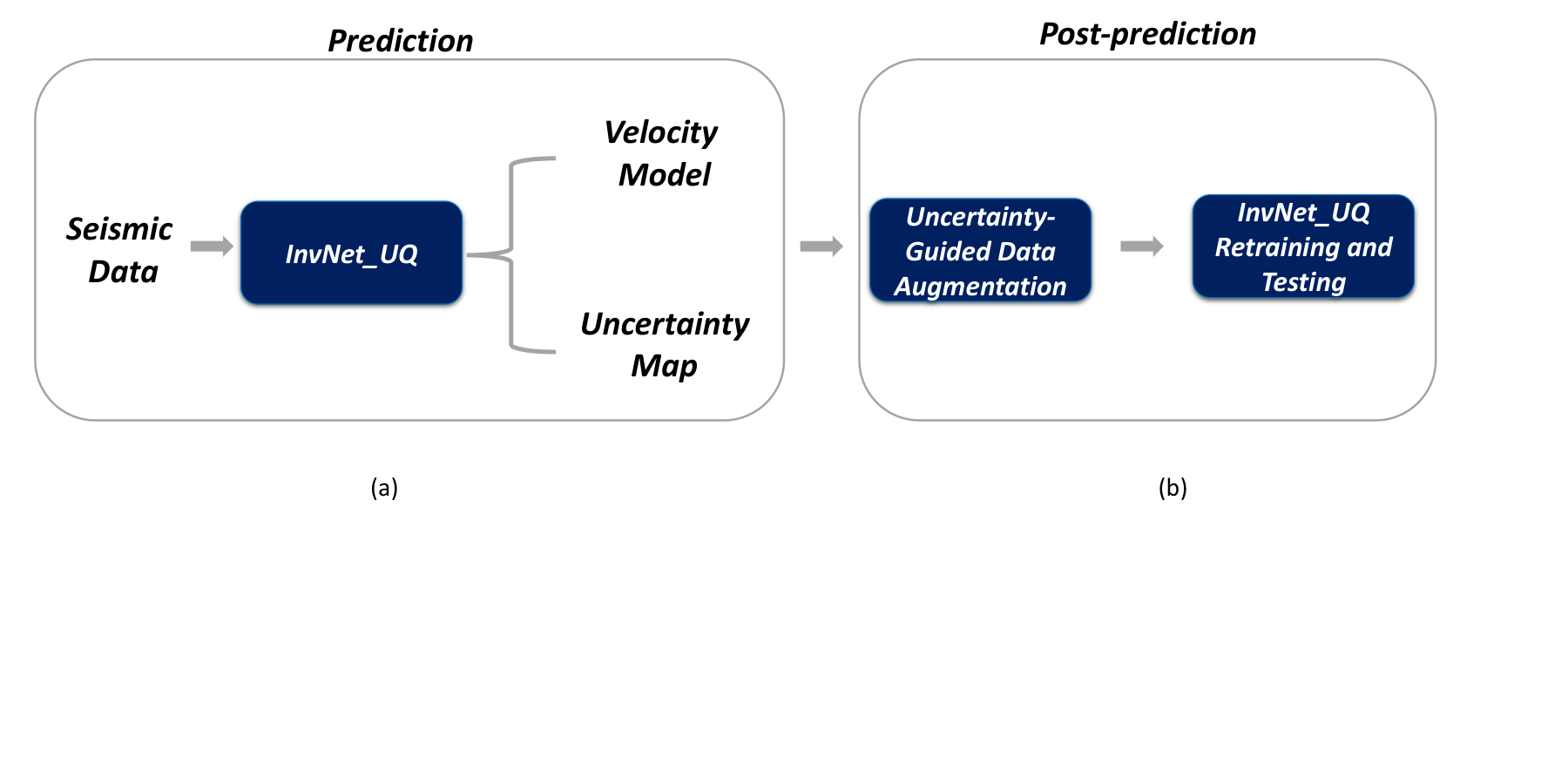
Figure 1 illustrates the developed workflow using the proposed probabilistic convolutional neural network (InvNet_UQ). First, InvNet_UQ is trained and applied to predict the velocity distributions at all quantile levels from the testing data. Meanwhile, the uncertainty map is calculated from two predictions at different quantile levels. Next, uncertainty-guided data augmentation is applied to all predicted velocity models from the testing data. Finally, the augmented data are added to the existing training data for retraining the network.
2.1 Simultaneous Quantile Regression
Uncertainty estimation is essential for seismic inversion for two reasons. First, seismic data contain different kinds of noise caused by the recording equipment, ambient disturbances, etc. Second, inversion is often ill-posed, which means that the solution can be nonunique or correspond to a local minimum of the objective function. Here, we estimate the uncertainty using the probabilistic neural based on the SQR proposed by Tagasovska and Lopez-Paz, 2019.
To solve the regression problem, we implement a neural network as a function to approximate the relationship between the input and output . To identify the network parameters, we minimize the mean-square error (MSE) between the prediction () and actual () values:
| (1) |
Therefore, the prediction () represents the conditional mean (expectation) of the prediction for a given input.
However, the expectation alone does not accurately reflect the data distribution. Therefore, quantile regression is proposed to analyze the prediction in a specific quantile (). One way to build such a model approximating the conditional quantile distribution function is to minimize the pinball loss ():
| (2) |
Indeed,
| (3) |
where is the strictly monotonic cumulative distribution function of the target variable taking real values . Consequently, denotes the quantile distribution function of the same variable for all quantile levels .
With pinball loss, Tagasovska and Lopez-Paz, 2019 propose employing Simultaneous Quantile Regression (SQR) to estimate all the quantile levels simultaneously by solving the following equation:
| (4) |
where are identically and independently distributed feature-target pairs drawn from the unknown probability distribution . Note that, unlike Bayesian neural networks, is not necessarily a Gaussian distribution. Then the estimated data uncertainty can be computed from the () prediction interval around the median:
| (5) |
where is the significance level.
2.2 Network architecture of InvNet_UQ
Following Wu and Lin, 2019, we use an encoder-decoder-based CNN to approximate the relationship between the input seismic data and the output velocity model. There are seven convolutional blocks with a kernel size of followed by a max pooling. Each block consists of a convolutional layer, batch normalization, and a tanh activation function. The high-dimensional data are reduced to a array in the latent space. These features are upsampled to the output size by eight decoder blocks containing a deconvolutional layer, batch normalization, and a LeakyRelu activation function. The end of the decoder is a central-cropping layer, which crops the output of the deconvolutional blocks to the desired size.
For the benchmark network (InversionNet), the loss function is the -norm of the difference between the prediction and the actual model. The input data size is , where the first number () is the number of channels (shot gathers). For each shot gather, there are 200 receivers recording for 4 s with a time interval of 4 ms. The output is a velocity model with a size of .
InvNet_UQ shares the same structure with InversionNet, but its loss function is computed using equation 4. To compute the SQR loss, first we randomly select six quantile levels () for each training epoch, and the selected is then fixed for every batch in the epoch. Then the computed six quantile losses are averaged to obtain the final loss. To incorporate quantile level into the neural network, every is extended to a tensor with the exact size of the seismic data and then added to the input data, so that the number of input channels of InvNet_UQ is increased to seven.
2.3 Uncertainty-guided data augmentation
Most existing UQ methods produce the variance of the prediction as the uncertainty map and abandon it after evaluating the prediction accuracy. In contrast, we propose a data-augmentation method to demonstrate the potential of the estimated uncertainty in improving the network performance. The idea of the method is to sample the uncertainty map and add it to the predicted velocity to obtain new velocity models :
| (6) |
where is the weight matrix applied to the computed uncertainty. Ideally, one needs to sample the uncertainty of every pixel with every weight in the range from 0 to 1 to find the actual velocity model. However, this procedure is impossible because it requires an infinite number of weight matrices to fully cover the range . To simplify the sampling process and ensure the effectiveness of the data-augmentation method, the weights should be randomly selected and have a minimum of 0 and maximum of 1.
An acoustic forward-modeling algorithm simulates seismic data for these new velocity models with the same settings used to generate the initial data. Then we add these new seismic-velocity pairs to the existing training data and retrain the network. Finally, the retrained network is applied to the testing data to estimate the velocity distribution. Because the new velocity models are generated using the prediction and the estimated uncertainty, they provide extra information that the model does not learn from the training data set. Moreover, the inclusion of these new models makes the training data more representative of the testing data distribution.
3 Results
3.1 Kimberlina data set
The proposed neural network with UQ is applied to monitoring and predicting migration using the synthetic Kimberlina data set. The Kimberlina reservoir model, generated by several institutions (Alumbaugh et al., 2021) as part of the U.S. Department of Energy “SMART Initiative” (U.S. Department of Energy, 2029), was built to simulate a potential commercial-scale geologic carbon storage in the Southern San Joaquin Basin of California (Wagoner, 2009), 30 km northwest of Bakersfield, CA, USA. The Kimberlina model has been released to the public to evaluate the effectiveness and robustness of different geophysical techniques for monitoring migration.
There is a total of 29 3D time-lapse P-wave velocity models (601 601 351 grid points) simulated for over 200 years. We slice the 3D velocity model along the axis to obtain the corresponding 2D models. The 2D velocity models from different slices have distinct velocity distributions, while those from the same slice (Figure 2) share the velocity field outside the reservoir, but inside the reservoir the velocity distribution is changed by the injected . To simulate the seismic data, we place six shots at the surface of the model, which has a grid size of 10 10 10 m.

The entire Kimberlina data set (1,537 velocity samples) is randomly divided into training (80) and testing (20) data. InverionNet and InvNetUQ are trained with the same data until they converge. Then these networks are applied to the testing data in different scenarios to predict the velocity distribution. To evaluate the predictions, we focus on three critical geologic structures (Figure 2; pointed by red arrows): the low-velocity layer immediately above the reservoir region (Zone 1), the three reservoirs (Zone 2), and the high-velocity dipping layer beneath the reservoirs (Zone 3).
3.2 Noise-free data
First, we test the trained networks on the original (perfect) testing data. The predictions (Figure 3) show that most features of the velocity model can be predicted by both InversionNet (Figure 3e-h) and InvNetUQ (Figure 3i-l) with sufficient accuracy, although there exists an area with larger errors. For example, compared with the actual model (Figure 3), both networks cannot accurately reconstruct the small plumes at year 1 (Figure 3a) because of the lack of training data at the beginning of the injection when the plumes are small. InversionNet tends to underestimate the size of the plumes (Figure 3e), while InvNetUQ is more likely to overestimate them (Figure 3i).

In addition, both methods could not reconstruct the bumps in the high-velocity dipping layer (circled by a dashed red line) and the anomaly in the low-velocity horizon above the reservoirs (circled by a solid red line) because of the lack of training data for these structures.
For the uncertainty map, the 95 prediction interval around the median is calculated from equation 5 by setting the prediction interval . We verify the uncertainty predicted by InvNetUQ (Figures 4e-h) by comparing it with the error map (Figures 4a-d). High uncertainty is observed around the low-velocity area above the reservoirs, especially near the anomaly (Zone 1) and the reservoir (Zone 2), as well as near the small bump in Zone 3, which matches the area with the most significant errors. The difference between the two confidence intervals, calculated from (Figure 4i-l), demonstrates the usefulness of the asymmetric uncertainty prediction, which cannot be provided by conventional UQ methods.
We also calculate the Pearson correlation between the absolute prediction error and the uncertainty and present the corresponding scatter plot in Figure 5. The Pearson correlation is , and the p-value is , which shows a strong positive correlation between the two variables. This correlation implies that the uncertainty is an accurate indicator of the prediction confidence, and indicates that InvNet_UQ can produce an uncertainty map sufficient to facilitate decision-making.


3.3 Influence of random noise
Next, the testing data are contaminated with Gaussian noise with the signal-to-noise ratio equal to 10 and 20. The noise is added only to the testing data, whereas the neural networks are still trained on noise-free samples. Here, we show only the prediction results for (SNR=10), which is more realistic for field data. Compared with the clean data (Figure 6a) where reflection events are apparent, reflections are not clearly visible in the noisy data (Figure 6b). Note that testing on noisy data is performed without fine-tuning the network.
Predictably, both networks produce more errors in the velocity field estimated from the noise-contaminated data (Figure 7). For the velocity model obtained by InversionNet (Figure 7a-d), significant distortions are observed in the low-velocity layer above the plumes (Zone 1), in the plumes themselves (Zone 2), and near the boundary between the reservoir and the deep high-velocity horizons (Zone 3). The plumes are barely visible, which would complicate monitoring injection.
In contrast, InvNetUQ (Figure 7e-h) reconstructs Zones 1 and 3 with sufficient resolution. The errors are mainly concentrated near the plumes in Zone 2, which is consistent with the calculated uncertainty map (Figure 7i-l). In addition, the noise does not significantly distort the predictions, which confirms that the proposed network remains robust for at least moderate noise levels.
The MSE (Figure 8) of the predictions by InversionNet jumps from for the clean data to for the noisy data (SNR=10). In contrast, there is only a slight increase in the MSE of InvNetUQ (i.e., from to ). Evidently, our method can handle noisy data with a realistic signal-to-noise ratio, and the noise does not distort the uncertainty quantification.


3.4 Influence of missing traces
Missing traces are typical in seismic surveys due to unavailable receivers and low SNR on some records. The commonly used remedies are reconstruction of the missing traces using interpolation and compressive sensing. However, accurate reconstruction usually takes a significant amount of time and is computationally costly. Therefore, next we test the effectiveness of InvNetUQ in dealing with the missing-data problem by randomly blocking 30 traces (Figures 9b) for every testing sample. The networks are trained with the complete seismic data. Hence, testing data that miss traces can be referred to as an “out-of-distribution” case.
Compared with the predicted results using the entire data set, both methods produce distortions in the velocity model due to the missing traces. InversionNet (Figures 10a-d) cannot predict the plume, while InvNetUQ (Figures 10e-h) still reconstructs these plumes with acceptable resolution. In addition, InvNetUQ is able to estimate the bottom right part of the velocity model, which is substantially distorted by InversionNet. Table 1 shows that our method is more robust and reduces MSE by about 30% compared with InversionNet.
The uncertainty for the upper part of the model (Figures 10i-l; marked by the red arrow) caused by the missing trace is significantly larger than that for the original data. Similar to the previous tests, the reservoirs generally have a higher uncertainty than other parts of the model.


| Conditions/Methods | InversionNet | InvNet_UQ | Augmented InvNet_UQ |
|---|---|---|---|
| Noise-free testing data | |||
| Testing data with 30% missing traces | |||
| Testing data with absence of low frequencies |
3.5 Influence of absent low-frequency data
Ultra-low-frequency seismic data are essential for the success of FWI, but they are seldom acquired in the field. Therefore, it is important to test the robustness of our algorithm in the absence of low frequencies (less than 3 Hz). We apply the Fourier transform to the perfect testing data and remove frequencies below 3 Hz with a Butterworth filter. Note that both neural networks are trained on the perfect training data that include the full frequency range.
Compared with the benchmark results, the velocity models produced by InversionNet are noticeably distorted (Figures 12a-d), even though the low frequencies do not dramatically influence the input seismic data (Figures 11). Specifically, InversionNet fails to reconstruct small plumes, which could be indicative of leakages. InvNet_UQ (Figures 12e-h) can still predict the plumes in the early stages of the injection with the resolution similar to that of the benchmark sections (Figures 3i-l), as revealed by the computed uncertainty map. The MSE also demonstrates that InvNet_UQ () remains robust compared to the perfect data and achieves higher resolution than InversionNet ().


3.6 Test of uncertainty-guided data augmentation
We augment the velocity models predicted from the perfect data (see equation 6). The uncertainty map is sampled with different weights, w=. Compared to the prediction (Figure 13b), the augmented data (Figure 13c-f) contain small plumes and bumps in Zone 3 (marked by the red arrows), which improves the prediction of these features. These newly generated data are used together with the existing training data to retrain InvNet_UQ. Then the trained network is applied to the testing data.

The testing loss of the perfect data shows that training on the augmented data reduces the MSE of the testing data from to , which demonstrates the effectiveness of our data augmentation method. The detailed comparison between the velocity map (Figures 14a-d) and the benchmark result (Figures 3i-l) shows that the network trained with the augmented data can improve the reconstruction of the velocity model. In particular, with the augmented data, the shape and amplitude of the predicted plumes are closer to those for the actual models, even in earlier years when the plumes are relatively small. In addition, the small bump in the high-velocity zone is captured more accurately. The calculated uncertainty further illustrates that the InvNet_UQ has a much higher accuracy in predicting the plumes (Zone 2), the low-velocity layer (Zone 3), the high-velocity dipping layer (Zone 1), and the upper part of the velocity model. Likewise, the ability of the proposed data-augmentation method to improve the prediction accuracy is demonstrated in the above tests for data with missing traces and missing low frequencies (Table 1).

4 Conclusions
We developed a convolutional neural network (CNN) with Simultaneous Quantile Regression (SQR) to predict the time-lapse velocity model and estimate the uncertainty map from the input seismic data. SQR is designed to build a network that estimates the conditional distributions of all pertinent quantiles utilizing the pinball loss. Then the uncertainty map is obtained from the prediction interval. In contrast to most conventional UQ methods, the uncertainty calculated here is related to the predicted velocity and has a physical meaning (i.e., the confidence interval). To fully utilize the computed uncertainty, we propose to employ data augmentation by sampling the uncertainty, adding the newly sampled data to the existing data set, and retraining the network. To benchmark the developed method, the pinball loss is replaced by the L1-norm objective function to form a deterministic neural network (InversionNet).
We test InvNetUQ on realistic synthetic data from the Kimberlina reservoir and compare the results with those from InversionNet. The results for clean data demonstrate that InvNetUQ can predict the velocity model with sufficient accuracy. The estimated uncertainty map is consistent with the error map, which implies that the uncertainty can be used to evaluate the prediction accuracy. The tests on data with noise, missing traces, etc. show that InvNetUQ remains robust and produces acceptable velocity maps, whereas the output of InversionNet is substantially distorted. This implies that the proposed method is applicable to field data and can facilitate confident decision-making. Retraining the network using the augmented data from the computed uncertainty improves the prediction accuracy, especially in areas with larger parameter variations including the plumes.
5 Acknowledgments
This work was funded by the U.S. Department of Energy (DOE) Office of Fossil Energy’s Carbon Storage Research Program via the Science-Informed Machine Learning to Accelerate Real Time Decision Making for Carbon Storage (SMART-CS) Initiative. Y. Liu and I. Tsvankin also acknowledge the support of the sponsors of the Center for Wave Phenomena (CWP) in the Department of Geophysics at Colorado School of Mines.
6 Author contributions statement
Youzuo Lin proposed and supervised the research. Yanhua Liu and Xitong Zhang conceived the design of the experiment(s). Yanhua Liu conducted the experiment(s). All authors contributed ideas to the project, analyzed the results, and reviewed the manuscript.
References
- Alumbaugh et al., (2021) Alumbaugh, D., M. Commer, D. Crandall, E. Gasperikova, S. Feng, W. Harbert, Y. Li, Y. Lin, S. Manthila Samarasinghe, and X. Yang, 2021, Development of a multi-scale synthetic data set for the testing of subsurface CO2 storage monitoring strategies: Presented at the American Geophysical Union (AGU 2021).
- Chen et al., (2018) Chen, B., D. R. Harp, Y. Lin, E. H. Keating, and R. J. Pawar, 2018, Geologic CO2 sequestration monitoring design: a machine learning and uncertainty quantification based approach: Applied energy, 225, 332–345.
- Feng et al., (2021) Feng, S., X. Zhang, B. Wohlberg, N. Symons, and Y. Lin, 2021, Monitoring and forecasting CO2 storage in the Sleipner area with spatio-temporal cnns: First International Meeting for Applied Geoscience & Energy Expanded Abstracts, 1686–1690.
- Furre et al., (2017) Furre, A. K., O. Eiken, H. Alnes, J. N. Vevatne, and A. F. Kiær, 2017, 20 years of monitoring -injection at Sleipner: Energy Procedia, 114, 3916–3926.
- Kim et al., (2010) Kim, J., Z. Xue, and T. Matsuoka, 2010, Experimental Study on Monitoring and Saturation with Combined P-wave Velocity and Resistivity: Presented at the . (SPE-130284-MS).
- Li et al., (2021) Li, D., S. Peng, Y. Guo, Y. Lu, and X. Cui, 2021, CO2 storage monitoring based on time-lapse seismic data via deep learning: International Journal of Greenhouse Gas Control, 108, 103336.
- Lin et al., (2022) Lin, Y., J. Theiler, and B. Wohlberg, 2022, Physics-guided data-driven seismic inversion: Recent progress and future opportunities in full waveform inversion: IEEE Signal Processing Magazine.
- Liu et al., (2022) Liu, Y., S. Feng, I. Tsvankin, D. Alumbaugh, and Y. Lin, 2022, Joint physics-based and data-driven time-lapse seismic inversion: Mitigating data scarcity: Geophysics, 0, 1–53.
- Lumley, (2010) Lumley, D., 2010, 4D seismic monitoring of sequestration: The Leading Edge, 29, no. 2, 150–155.
- Pevzner et al., (2017) Pevzner, R., M. Urosevic, D. Popik, V. Shulakova, K. Tertyshnikov, E. Caspari, J. Correa, T. Dance, A. Kepic, S. Glubokovskikh, S. Ziramov, B. Gurevich, R. Singh, M. Raab, M. Watson, T. Daley, M. Robertson, and B. Freifeld, 2017, 4D surface seismic tracks small supercritical injection into the subsurface: CO2CRC Otway Project: International Journal of Greenhouse Gas Control, 63, 150–157.
- Ren et al., (2021) Ren, P., Y. Xiao, X. Chang, P.-Y. Huang, Z. Li, B. B. Gupta, X. Chen, and X. Wang, 2021, A survey of deep active learning: ACM Computing Surveys, 54.
- Tagasovska and Lopez-Paz, (2019) Tagasovska, N., and D. Lopez-Paz, 2019, in Single-Model Uncertainties for Deep Learning: Curran Associates Inc.
- Tang et al., (2022) Tang, M., X. Ju, and L. J. Durlofsky, 2022, Deep-learning-based coupled flow-geomechanics surrogate model for CO2 sequestration: International Journal of Greenhouse Gas Control, 118, 103692.
- Um et al., (2022) Um, E. S., D. Alumbaugh, Y. Lin, and S. Feng, 2022, Real-time deep-learning inversion of seismic full waveform data for CO2 saturation and uncertainty in geological carbon storage monitoring: Geophysical Prospecting, n/a.
- U.S. Department of Energy, (2029) U.S. Department of Energy, 2019 - 2029, Science-informed machine learning for accelerating real-time decisions in subsurface applications (smart) initiative.
- Wagoner, (2009) Wagoner, J., 2009, 3D geologic modeling of the southern San Joaquin basin for the Westcarb Kimberlina Demonstration Project- a status report: Technical report.
- Wu and Lin, (2019) Wu, Y., and Y. Lin, 2019, InversionNet: An efficient and accurate data-driven full waveform inversion: IEEE Transactions on Computational Imaging, 6, 419–433.
- Zhang and Lin, (2020) Zhang, Z., and Y. Lin, 2020, Data-driven seismic waveform inversion: A study on the robustness and generalization: IEEE Transactions on Geoscience and Remote Sensing, 58, 6900–6913.