跳到论文正文
W Papers独立论文阅读器 arXiv:2212.04485 论文正文 计算阅读时间 · 0%
引用这篇论文根据当前论文元数据生成,正式投稿前建议核对。


License: CC BY 4.0
arXiv:2212.04485v2 [astro-ph.CO] 16 Feb 2023

A roadmap to cosmological parameter analysis with third-order shear statistics II: Analytic covariance estimate The modelling code is available at https://github.com/sheydenreich/threepoint/releases.

Laila Linke Affiliation: Argelander-Institut für Astronomie, Auf dem Hügel 71, 53121 Bonn, Germany Email: llinke@astro.uni-bonn.de    Sven Heydenreich Affiliation: Argelander-Institut für Astronomie, Auf dem Hügel 71, 53121 Bonn, Germany Email: llinke@astro.uni-bonn.de    Pierre A. Burger Affiliation: Argelander-Institut für Astronomie, Auf dem Hügel 71, 53121 Bonn, Germany Email: llinke@astro.uni-bonn.de    Peter Schneider Affiliation: Argelander-Institut für Astronomie, Auf dem Hügel 71, 53121 Bonn, Germany Email: llinke@astro.uni-bonn.de
Version August 11, 2026; received xxx, accepted yyy
Abstract

Context. Third-order weak lensing statistics are a promising tool for cosmological analyses since they extract cosmological information in the non-Gaussianity of the cosmic large-scale structure. However, such analyses require precise and accurate models for the covariance of the statistics.

Aims. In this second paper of a series on third-order weak lensing statistics, we derive and validate an analytic model for the covariance of the third-order aperture statistics ⟨Map3⟩\expectationvalue{\Map^3}.

Methods. We derive the covariance model from a real-space estimator for ⟨Map3⟩\expectationvalue{\Map^3}, including the Gaussian and non-Gaussian parts. We validate the model by comparing it to estimates from simulated Gaussian random fields (GRFs) and two sets of NN-body simulations. Finally, we perform mock cosmological analyses with the model covariance and the simulation estimate to compare the resulting parameter constraints.

Results. We find good agreement between the analytic model and the simulations, both for the GRFs and the NN-body simulations. The figure of merit in the S8S_{8}-Ωm\Omega_{\mathrm{m}} plane from our covariance model is within 3% of the one obtained from the simulated covariances. We also show that our model, which is based on an estimator using convergence maps, can be used to obtain upper and lower bounds for the covariance of an estimator based on three-point shear correlation functions. This second estimator is required to measure ⟨Map3⟩\expectationvalue{\Map^3} in realistic survey data. In our derivation, we find that the covariance of ⟨Map3⟩\expectationvalue{\Map^3} cannot be obtained from the bispectrum covariance and that it includes several ‘finite-field terms’ that do not scale with the inverse survey area.

Conclusions. Our covariance model is sufficiently accurate for analysing stage III surveys. Covariances for statistics in Fourier space cannot always be straightforwardly converted into covariance for real-space statistics.

Key Words.
gravitational lensing – weak, cosmology – cosmological parameters, methods – statistical, methods – analytical, large-scale structure of Universe

1 Introduction

Using weak gravitational lensing of the cosmic large-scale structure (LSS) has become a precise and accurate method to infer cosmological parameters (Heymans et al. 2021, Hikage et al. 2019, Abbott et al. 2022). Weak-lensing analyses have mainly concentrated on second-order statistics, such as shear two-point correlation functions or galaxy-galaxy-lensing. However, since the cosmic LSS is non-Gaussian, second-order statistics do not contain its total information content. To access the additional information, higher-order statistics (HOS) are needed. These HOS depend on cosmological parameters differently than second-order statistics, so they can be used to break degeneracies (Takada & Jain 2004, Kilbinger & Schneider 2005, Kayo et al. 2013) or constrain nuisance parameters such as galaxy bias or intrinsic alignment (Pyne & Joachimi 2021, Troxel & Ishak 2012).

Many HOS have been suggested to complement second-order analyses, for example, peak statistics (Kacprzak et al. 2016, Zürcher et al. 2021 Martinet et al. 2021), density split statistics (Friedrich et al. 2018, Gruen et al. 2018, Burger et al. 2022), or persistent homology (Heydenreich et al. 2021; Heydenreich et al. 2022a). Most of these statistics, though, cannot be modelled from analytical theories and instead require time-consuming realistic NN-body simulations. Additionally, for many HOS, the measurement requires converting weak lensing shear estimates to mass convergence maps. This conversion becomes complicated in the presence of masks and for finite survey areas, which can lead to biased estimators (Seitz & Schneider 1996).

In this series of papers, we are considering the third-order aperture mass ⟨Map3⟩\expectationvalue{\Map^3}, which is not affected by these problems. It is linearly related to the third-order shear correlation functions Γi\Gamma_{i} (Jarvis et al. 2004, Schneider et al. 2005), which can be directly measured in shear catalogues and converted into ⟨Map3⟩\expectationvalue{\Map^3}. This was demonstrated recently by Secco et al. 2022, who measured ⟨Map3⟩\expectationvalue{\Map^3} with high significance from the Dark Energy Survey Year 3 shear catalogues. Moreover, in contrast to many other HOS, ⟨Map3⟩\expectationvalue{\Map^3} and Γi\Gamma_{i} can be modelled analytically without directly relying on simulations.

There are several advantages to using ⟨Map3⟩\expectationvalue{\Map^3} instead of Γi\Gamma_{i}, among them that ⟨Map3⟩\expectationvalue{\Map^3} compress the information in the Γi\Gamma_{i} from a data vector with thousands of entries to one containing only tens of entries in a non-tomographic setup, and that the ⟨Map3⟩\expectationvalue{\Map^3} have a clear separation into EE- and BB-modes, allowing for the detection of untreated systematic effects. Our goal is to lay the groundwork for a cosmological analysis with ⟨Map3⟩\expectationvalue{\Map^3}. Such an analysis requires two ingredients: a model of ⟨Map3⟩\expectationvalue{\Map^3} and an estimate of its covariance matrix. The first ingredient is the subject of Heydenreich et al. 2022b, where we present and test an analytic model of ⟨Map3⟩\expectationvalue{\Map^3} based on the BiHalofit bispectrum model (Takahashi et al. 2020). Here, we are concerned with the second ingredient, which is the covariance.

The covariance of the estimator of a statistic can be obtained in three ways. The first possibility is applying the estimator to a large set of (quasi-)independent cosmological NN-body simulations and using the sample covariance of the estimates. However, an unbiased and precise estimate requires many more realisations than entries in the data vector. For example, for a tomographic analysis of ⟨Map3⟩\expectationvalue{\Map^3} with four redshift bins and four different scale radii, the data vector contains 400 entries, so hundreds of simulations are needed for a simulated covariance estimate. Such an estimate would be very time-consuming, as both the creation of this many independent simulations and the measurement of ⟨Map3⟩\expectationvalue{\Map^3} in them is computationally demanding. The second possibility is to estimate the covariance directly from the data using jackknife resampling or bootstrap methods. For this, the survey area is divided into smaller patches, the statistics are estimated separately on each of these patches, and the sample covariance of these individual estimates is taken as the covariance estimate. However, this method has two main disadvantages. First, information on correlations larger than the patch size is lost. Since the number of patches must be at least as large as the length of the data vector, the required number of patches becomes large and their size small. Second, the method implicitly assumes that the individual patches are independent of each other. This assumption is not true, in particular, if small, neighbouring patches are considered. This causes biases in the covariance estimate. Third, triplets covering two or three patches need to be neglected for the estimation of the data vector. Otherwise, the covariance from jackknife or bootstrap resampling would overestimate the true covariance of the data.

Instead, cosmic shear covariances can also be calculated analytically for a given estimator. This was done, for example, for two-point statistics (Joachimi et al. 2008) or the matter bispectrum (Joachimi et al. 2009). While the derivation of an expression for a covariance can be tedious, once it is done, evaluating them for the characteristics of a specific survey is usually accurate and quick, at least compared to running hundreds of cosmological simulations. It is also easier to infer the dependence of the covariance on survey area and geometry from an analytic expression. Consequently, we follow this approach and derive an analytical expression for the covariance of ⟨Map3⟩\expectationvalue{\Map^3}. We test our result by comparing it with the covariance measured in simulated mock data, both simple Gaussian shear fields and full cosmological simulations, and investigate the influence of different terms in the covariance by performing mock cosmological analyses.

In our derivation, we make five crucial findings. First, the covariance consists of six terms, two of which belong to the Gaussian part and four to the non-Gaussian part. These terms all depend on the survey area and window function (Sect. 3.1 and 3.2). Second, the individual covariance terms can be estimated from correlation functions of the aperture mass map. These correlation functions need to be known only on scales inside the survey area (Sect. 3.3). Third, under the ‘large-field approximation’, which assumes a broad survey window function, two covariance terms vanish, while the others scale inversely with the survey area. The vanishing terms decrease faster than 1/A1/A with survey area AA. We refer to them as finite-field terms. One of these terms is already present for Gaussian fields (Sect. 3.4). Fourth, the covariance of ⟨Map3⟩\expectationvalue{\Map^3} cannot be obtained from the bispectrum covariance unless the large-field approximation is valid. Using a linear transformation of the covariance of a Fourier space quantity to obtain the covariance for a real-space observable has been done for second-order statistics (Joachimi et al. 2021; Friedrich et al. 2021). However, for ⟨Map3⟩\expectationvalue{\Map^3} this approach already fails for Gaussian fields if the large-field approximation is not used (Sect. 4). Finally, our covariance model, based on an estimator using convergence maps, can be used to obtain upper and lower limits on the covariance for an estimator based on third-order shear correlation functions (Sect. 5.3.2).

This paper is structured as follows. In Sect. 2 we give a short overview of third-order shear statistics, and we introduce our notation, the third-order aperture mass ⟨Map3⟩\expectationvalue{\Map^3}, and its estimator. We derive the covariance of this estimator in Sect. 3. In Sect. 4 we show that an alternative derivation of the ⟨Map3⟩\expectationvalue{\Map^3} covariance from the bispectrum covariance is not correct. We validate the model by comparing its predictions to simulated data in Sect. 5. Finally, in Sect. 6, we perform mock cosmological analyses to compare the results from the validation data to our model and investigate the impact of the individual covariance terms. We conclude with a summary and discussion in Sect. 7. Throughout this paper, we assume a spatially flat universe. Our covariance modelling code is publically available 11 1 https://github.com/sheydenreich/threepoint/releases.

2 Theoretical background

In this section, we briefly review some fundamental weak lensing quantities relevant to third-order shear statistics and the covariance calculation in the remainder of this work. We refer to Bartelmann & Schneider 2001; Hoekstra & Jain 2008 or Bartelmann 2010 for in-depth reviews on weak lensing.

One of the fundamental quantities in weak gravitational lensing is the convergence κ⁡(ϑ)\kappa(\bm{\vartheta}), which is the normalised surface mass density at angular position ϑ\bm{\vartheta}. In a flat universe, it is related to the density contrast δ⁡(χ​ϑ,χ)\delta(\chi\bm{\vartheta},\chi) at angular position ϑ\bm{\vartheta} and comoving distance χ\chi via

κ⁡(ϑ)=3​H02​Ωm2​c2​∫0∞dχ​q​(χ)​δ⁡(χ​ϑ,χ)a⁡(χ),where ​q​(χ)=∫χ∞dχ′​p​(χ′)​χ′−χχ′,\kappa(\bm{\vartheta})=\frac{3H_{0}^{2}\Omega_{\mathrm{m}}}{2c^{2}}\int_{0}^{\infty}\differential{\chi}\;q(\chi)\,\frac{\delta(\chi\bm{\vartheta},\chi)}{a(\chi)}\;,\textrm{where }q(\chi)=\int_{\chi}^{\infty}\differential{\chi'}\,p(\chi^{\prime})\,\frac{\chi^{\prime}-\chi}{\chi^{\prime}}\;, (1)

with the Hubble constant H0H_{0}, the matter density parameter Ωm\Omega_{\mathrm{m}}, the speed-of-light cc, the cosmic scale factor a⁡(χ)a(\chi) at χ\chi, normalised to unity today, and the probability distribution p⁡(χ)​dχp(\chi)\,\differential{\chi} of source galaxies in comoving distance.

We treat κ⁡(ϑ)\kappa(\bm{\vartheta}) as a homogenous and isotropic random field, which is characterised by the full set of its polyspectra 𝒫n\mathcal{P}_{n}, defined by

⟨κ~​(ℓ1)​…​κ~​(ℓn)⟩c=𝒫n​(ℓ1,…,ℓn)​(2​π)2​δD​(ℓ1+⋯+ℓn),\expectationvalue{\tilde{\kappa}(\ellvec_1)\dots\tilde{\kappa}(\ellvec_n)}_{\mathrm{c}}=\mathcal{P}_{n}(\bm{\ell}_{1},\dots,\bm{\ell}_{n})\,(2\pi)^{2}\,\delta_{\mathrm{D}}(\bm{\ell}_{1}+\dots+\bm{\ell}_{n})\;, (2)

where κ~​(ℓ)\tilde{\kappa}(\bm{\ell}) is the Fourier transform of κ\kappa and the ⟨…⟩c\expectationvalue{\dots}_{\mathrm{c}} are connected correlation functions. Interesting for us in this work is the powerspectrum PP, bispectrum BB, trispectrum TT, and the pentaspectrum P6P_{6}, defined as

P⁡(ℓ)=P2​(ℓ,−ℓ),B⁡(ℓ1,ℓ2)=𝒫n​(ℓ1,ℓ2,−ℓ1−ℓ2),T⁡(ℓ1,ℓ2,ℓ3)=𝒫n​(ℓ1,ℓ2,ℓ3,−ℓ1−ℓ2−ℓ3),\displaystyle P(\ell)=P_{2}(\bm{\ell},-\bm{\ell})\,,\quad B(\bm{\ell}_{1},\bm{\ell}_{2})=\mathcal{P}_{n}(\bm{\ell}_{1},\bm{\ell}_{2},-\bm{\ell}_{1}-\bm{\ell}_{2})\,,\quad T(\bm{\ell}_{1},\bm{\ell}_{2},\bm{\ell}_{3})=\mathcal{P}_{n}(\bm{\ell}_{1},\bm{\ell}_{2},\bm{\ell}_{3},-\bm{\ell}_{1}-\bm{\ell}_{2}-\bm{\ell}_{3})\,, (3)

and

P6​(ℓ1,ℓ2,ℓ3,ℓ4,ℓ5)=𝒫n​(ℓ1,ℓ2,ℓ3,ℓ4,ℓ5,−ℓ1−ℓ2−ℓ3−ℓ4−ℓ5).\displaystyle P_{6}(\bm{\ell}_{1},\bm{\ell}_{2},\bm{\ell}_{3},\bm{\ell}_{4},\bm{\ell}_{5})=\mathcal{P}_{n}(\bm{\ell}_{1},\bm{\ell}_{2},\bm{\ell}_{3},\bm{\ell}_{4},\bm{\ell}_{5},-\bm{\ell}_{1}-\bm{\ell}_{2}-\bm{\ell}_{3}-\bm{\ell}_{4}-\bm{\ell}_{5})\;. (4)

The κ\kappa-polyspectra of are related to the polyspectra 𝒫n(3​d)\mathcal{P}_{n}^{\mathrm{(3d)}} of the three-dimensional density contrast δ\delta, using the Limber-approximation (Kaiser & Jaffe 1997; Kayo et al. 2013),

𝒫n​(ℓ1,…,ℓn)\displaystyle\mathcal{P}_{n}(\bm{\ell}_{1},\dots,\bm{\ell}_{n}) =(3​H02​Ωm2​c2)n​∫0∞dχ​qn​(χ)χn−2​a​(χ)n​𝒫n(3​d)​(ℓ1/χ,…,ℓn/χ,χ).\displaystyle=\left(\frac{3H_{0}^{2}\Omega_{\mathrm{m}}}{2c^{2}}\right)^{n}\,\int_{0}^{\infty}\differential{\chi}\;\frac{q^{n}(\chi)}{\chi^{n-2}\,a(\chi)^{n}}\,\mathcal{P}_{n}^{\mathrm{(3d)}}(\bm{\ell}_{1}/\chi,\dots,\bm{\ell}_{n}/\chi,\chi)\;. (5)

We model the three-dimensional power spectrum with the revised Halofit prescription by Takahashi et al. 2012 and the three-dimensional bispectrum with BiHalofit (Takahashi et al. 2020). For the tri- and pentaspectrum, we use the halo model (Cooray & Sheth 2002) with a Sheth–Tormen halo mass function and halo bias (Sheth & Tormen 1999) and Navarro–Frenk–White-halo profiles. To simplify our calculation, we use only the 1-halo term for the trispectrum, which we expect to be dominant at the considered ℓ\ell-scales. For the pentaspectrum, we use the 1- and part of the 2-halo term (see Sect. 3.4 and Appendix C)

The convergence cannot be directly observed, but it is related to the weak lensing shear γ\gamma, which describes the change in the observed ellipticity of source galaxies due to the lensing effect. For third-order shear statistics, we are interested in the three-point correlation function of the shear, whose so-called natural components Γi\Gamma_{i} were derived by Schneider & Lombardi 2003. However, these components are challenging to handle in practice since they require a large number of bins (typically of the order of 10310^{3}) and are complex to model because they relate to the matter bispectrum via multi-dimensional integrals involving oscillating Bessel functions. As shown in 15, more practical quantities with similar information content are the third-order aperture statistics ⟨Map3⟩\expectationvalue{\Map^3}.

Aperture statistics are moments of the aperture mass MapM_{\mathrm{ap}}, a smoothed convergence map, which depends on its position α\mathbf{\alpha} and a characteristic smoothing scale θ\theta,

Map​(α,θ)=∫d2ϑ​Uθ​(|α−ϑ|)​κ​(ϑ), with ​Uθ​(ϑ)=1θ2​u​(ϑθ),M_{\mathrm{ap}}(\mathbf{\alpha},\theta)=\int\differential[2]{\vartheta}\;U_{\theta}(|\mathbf{\alpha}-\bm{\vartheta}|)\,\kappa(\bm{\vartheta})\;,\textrm{ with }U_{\theta}(\vartheta)=\frac{1}{\theta^{2}}\,u\left(\frac{\vartheta}{\theta}\right)\;, (6)

where UθU_{\theta} is a filter function with aperture scale radius θ\theta. As long as this is a compensated filter function, meaning ∫dϑ​ϑ​Uθ​(ϑ)=0,\int\differential{\vartheta}\vartheta\,U_{\theta}(\vartheta)=0\;, the aperture mass can be estimated from the tangential shear γt\gamma_{\mathrm{t}} instead of the convergence (Schneider 1996),

Map​(α,θ)=∫d2ϑ​Qθ​(|α−ϑ|)​γt​(α,ϑ),withQθ​(ϑ)=2ϑ2​∫0ϑdϑ′​ϑ′​Uθ​(ϑ′)−Uθ​(ϑ).M_{\mathrm{ap}}(\mathbf{\alpha},\theta)=\int\differential[2]{\vartheta}\;Q_{\theta}(|\mathbf{\alpha}-\bm{\vartheta}|)\,\gamma_{\mathrm{t}}(\mathbf{\alpha};\bm{\vartheta})\;,\quad\textrm{with}\quad Q_{\theta}(\vartheta)=\frac{2}{\vartheta^{2}}\,\int_{0}^{\vartheta}\differential{\vartheta'}\;\vartheta^{\prime}U_{\theta}(\vartheta^{\prime})-U_{\theta}(\vartheta)\;. (7)

Here, we are interested in the covariance of the third-order aperture statistics ⟨Map3⟩\expectationvalue{\Map^3}, given by

⟨Map3⟩⁡(θ1,θ2,θ3)=⟨Map​(α,θ1)​Map​(α,θ2)​Map​(α,θ3)⟩,\expectationvalue{\Map^3}(\theta_{1},\theta_{2},\theta_{3})=\expectationvalue{\Map(\alphavec, \theta_1)\,\Map(\alphavec, \theta_2)\,\Map(\alphavec, \theta_3)}\,, (8)

which is our main observable for third-order shear statistics. ⟨Map3⟩\expectationvalue{\Map^3} is related to the convergence bispectrum by

⟨Map3⟩⁡(θ1,θ2,θ3)\displaystyle\expectationvalue{\Map^3}(\theta_{1},\theta_{2},\theta_{3}) =∫d2ℓ1(2​π)2​∫d2ℓ2(2​π)2​u~​(ℓ1​θ1)​u~​(ℓ2​θ2)​u~​(|ℓ1+ℓ2|​θ3)​B​(ℓ1,ℓ2).\displaystyle=\int\frac{\differential[2]{\ell_1}}{(2\pi)^{2}}\int\frac{\differential[2]{\ell_2}}{(2\pi)^{2}}\;\tilde{u}(\ell_{1}\,\theta_{1})\,\tilde{u}(\ell_{2}\,\theta_{2})\,\tilde{u}\left(|\bm{\ell}_{1}+\bm{\ell}_{2}|\,\theta_{3}\right)\,B(\bm{\ell}_{1},\bm{\ell}_{2})\;. (9)

For the comparison of the analytical covariance to mock data in Sect. 5 and the estimate of the cosmological parameter analysis in Sect. 6 we choose the exponential filter function from Crittenden et al. 2002,

u​(x)=12​π​(1−x22)​exp⁡(−x22).u(x)=\frac{1}{2\pi}\,\left(1-\frac{x^{2}}{2}\right)\,\exp(-\frac{x^2}{2})\;. (10)

The normalisation of the aperture filter functions is chosen such that ∫d2​ϑ​Q​(ϑ)=1\int d^{2}\vartheta Q(\mathbf{\vartheta})=1.

A′A^{\prime}AAα\mathbf{\alpha}θ\thetaα′\mathbf{\alpha}^{\prime}θ\theta
Figure 1: Illustration of aperture mass estimation. The area A′A^{\prime} is the size of the full convergence field, on which we place apertures with scale radius θ\theta, illustrated by the circles, to obtain Map​(α,θ)M_{\mathrm{ap}}(\mathbf{\alpha},\theta). Apertures centred on positions α\mathbf{\alpha} within the smaller area AA lie completely within A′A^{\prime}, while apertures centred on positions α′\mathbf{\alpha}^{\prime} outside of AA extend outside of A′A^{\prime}, so Map​(α′,θ)M_{\mathrm{ap}}(\mathbf{\alpha}^{\prime},\theta) is biased.

Based on Eq. (6), Map​(α,θ)M_{\mathrm{ap}}(\mathbf{\alpha},\theta) can be estimated from convergence fields using

M^ap​(α,θ)=∫A′d2ϑ​Uθ​(|α−ϑ|)​κ​(ϑ),\hat{M}_{\mathrm{ap}}(\mathbf{\alpha},\theta)=\int_{A^{\prime}}\differential[2]{\vartheta}U_{\theta}(|\mathbf{\alpha}-\bm{\vartheta}|)\,\kappa(\bm{\vartheta})\;, (11)

where A′A^{\prime} is the full area of the convergence field κ\kappa. This estimator can be visualised as placing an aperture of radius θ\theta centred at position α\mathbf{\alpha} and averaging the convergence values within the aperture weighted by the filter function UθU_{\theta} (see Fig. 1). The ⟨Map3⟩⁡(θ1,θ2,θ3)\expectationvalue{\Map^3}(\theta_{1},\theta_{2},\theta_{3}) can then be estimated by averaging the product of the M^ap​(α,θ)\hat{M}_{\mathrm{ap}}(\mathbf{\alpha},\theta) for the three filter radii over the aperture positions α\mathbf{\alpha}. However, for α\mathbf{\alpha} close to the border of the survey area, M^ap​(α,θ)\hat{M}_{\mathrm{ap}}(\mathbf{\alpha},\theta) is biased because the aperture includes regions outside the survey where κ\kappa is not known. Consequently, for an unbiased estimate of ⟨Map3⟩\expectationvalue{\Map^3}, we only average over an area AA smaller than A′A^{\prime}, which leads to the estimator

M^ap3​(θ1,θ2,θ3)\displaystyle\hat{M}_{\mathrm{ap}}^{3}(\theta_{1},\theta_{2},\theta_{3}) =1A​∫Ad2α​∏i=13∫A′d2ϑi​Uθi​(|α−ϑi|)​κ​(ϑi).\displaystyle=\frac{1}{A}\int_{A}\differential[2]{\alpha}\,\prod_{i=1}^{3}\int_{A^{\prime}}\differential[2]{\varthetavec_i}U_{\theta_{i}}(|\mathbf{\alpha}-\bm{\vartheta}_{i}|)\,\kappa(\bm{\vartheta}_{i})\,. (12)

We have assumed here that apertures are placed densely so that the separation between aperture centres is much smaller than the aperture radius θ\theta, to use a continuous integral over α\mathbf{\alpha} instead of a sum. If A′A^{\prime} is large enough that all UθU_{\theta} centred on points within AA vanish outside of A′A^{\prime}, we can replace A′A^{\prime} with the full ℝ2\mathbb{R}^{2}. We also introduce the survey window function WA​(α)W_{A}(\mathbf{\alpha}), which is unity for α\mathbf{\alpha} inside AA and zero otherwise. With WW, we convert integrals over AA into integrals over ℝ2\mathbb{R}^{2}, which we denote as two-dimensional integrals without integration borders in the following. The estimator for ⟨Map3⟩\expectationvalue{\Map^3} becomes

M^ap3​(θ1,θ2,θ3)\displaystyle\hat{M}_{\mathrm{ap}}^{3}(\theta_{1},\theta_{2},\theta_{3}) =1A​∫d2α​WA​(α)​[∏i=13∫d2ϑi​Uθi​(|α−ϑi|)​κ​(ϑi)].\displaystyle=\frac{1}{A}\,\int\differential[2]{\alpha}\,W_{A}(\mathbf{\alpha})\,\left[\prod_{i=1}^{3}\int\differential[2]{\varthetavec_i}U_{\theta_{i}}(|\mathbf{\alpha}-\bm{\vartheta}_{i}|)\,\kappa(\bm{\vartheta}_{i})\right]\;. (13)

This estimator is easily applied to simulations, where convergence maps without masks are available (see Sect. 5.2.1). However, this estimator should not be used for survey data that includes masked areas. In that case, one would instead measure the correlation functions Γi\Gamma_{i} and convert these into ⟨Map3⟩\expectationvalue{\Map^3} (15, see the discussion in Section 5.3 of). In this approach, one does not need to decrease the survey area from A′A^{\prime} to AA because no apertures are laid down. Therefore, the covariance for this estimator is smaller than the covariance for the M^ap3\hat{M}_{\mathrm{ap}}^{3} in Eq. (13). However, the unbiased construction of the aperture mass on the whole area A′A^{\prime} requires shear estimates outside of A′A^{\prime} as well. Therefore, even Γi\Gamma_{i} measured from shear estimates on all of A′A^{\prime} cannot include the full information that would be contained in an unbiased estimate of M^ap3\hat{M}_{\mathrm{ap}}^{3} on A′A^{\prime}. Consequently, in the absence of masked regions, we expect the magnitude of the covariance for the estimator based on the Γi\Gamma_{i} to be between the covariance for M^ap3\hat{M}_{\mathrm{ap}}^{3} for a survey area of AA and a survey area of A′A^{\prime}. We verify this expectation in Sect. 5.

3 Derivation of aperture statistics covariance from the real-space estimator

We now derive the covariance CM^ap3C_{\hat{M}_{\mathrm{ap}}^{3}} of M^ap3\hat{M}_{\mathrm{ap}}^{3}. An overview of our calculation is given in Fig. 2, with references to the main equations in our derivation. In the derivation, we find that the covariance comprises several terms, including various permutations of scale radii. For simplicity, we write here ‘Perm.’ to indicate permutations; the complete list of permutations for all terms is given in Appendix A. We are not explicitly addressing the effect of shape noise in this section, but shape noise can be easily included in the derived expressions by replacing the power spectrum PP with P+σϵ2/2​nP+{\sigma_{\epsilon}^{2}}/{2n}, where nn is the galaxy number density and σϵ2\sigma^{2}_{\epsilon} the two-component ellipticity dispersion. We show the validity of this treatment in Appendix B.

CM^ap3{\lx@inpgf@ignorespaces C_{\hat{M}_{\mathrm{ap}}^{3}}}={\lx@inpgf@ignorespaces=}⟨M^ap3​M^ap3⟩{\lx@inpgf@ignorespaces\Big\langle\hat{M}_{\mathrm{ap}}^{3}\hat{M}_{\mathrm{ap}}^{3}\Big\rangle}−{\lx@inpgf@ignorespaces-}⟨M^ap3⟩​⟨M^ap3⟩{\lx@inpgf@ignorespaces\Big\langle\hat{M}_{\mathrm{ap}}^{3}\Big\rangle\Big\langle\hat{M}_{\mathrm{ap}}^{3}\Big\rangle}⟨M^ap3​M^ap3⟩G{\lx@inpgf@ignorespaces\Big\langle\hat{M}_{\mathrm{ap}}^{3}\hat{M}_{\mathrm{ap}}^{3}\Big\rangle_{\mathrm{G}}}⟨M^ap3​M^ap3⟩BB{\lx@inpgf@ignorespaces\Big\langle\hat{M}_{\mathrm{ap}}^{3}\hat{M}_{\mathrm{ap}}^{3}\Big\rangle_{\mathrm{BB}}}⟨M^ap3​M^ap3⟩PT{\lx@inpgf@ignorespaces\Big\langle\hat{M}_{\mathrm{ap}}^{3}\hat{M}_{\mathrm{ap}}^{3}\Big\rangle_{\mathrm{PT}}}⟨M^ap3​M^ap3⟩P6{\lx@inpgf@ignorespaces\Big\langle\hat{M}_{\mathrm{ap}}^{3}\hat{M}_{\mathrm{ap}}^{3}\Big\rangle_{\mathrm{P_{6}}}}TP​P​P,1​, Eq. (20){\lx@inpgf@ignorespaces T_{PPP,1}\textrm{, Eq.\penalty\ \eqref{eq: T1 final}}}TP​P​P,2​, Eq. (21){\lx@inpgf@ignorespaces T_{PPP,2}\textrm{, Eq.\penalty\ \eqref{eq: T2 final}}}⟨M^ap3⟩​⟨M^ap3⟩{\lx@inpgf@ignorespaces\Big\langle\hat{M}_{\mathrm{ap}}^{3}\Big\rangle\Big\langle\hat{M}_{\mathrm{ap}}^{3}\Big\rangle}TB​B​, Eq. (27){\lx@inpgf@ignorespaces T_{BB}\textrm{, Eq.\penalty\ \eqref{eq: T4 final}}}TP​T,1​, Eq. (29){\lx@inpgf@ignorespaces T_{PT,1}\textrm{, Eq.\penalty\ \eqref{eq: T5 final}}}TP​T,2​, Eq. (30){\lx@inpgf@ignorespaces T_{PT,2}\textrm{, Eq.\penalty\ \eqref{eq: T6 final}}}TP6​, Eq. (32){\lx@inpgf@ignorespaces T_{P_{6}}\textrm{, Eq.\penalty\ \eqref{eq: T7 final}}}TP​P​P,1∞​, Eq. (44){\lx@inpgf@ignorespaces T_{PPP,1}^{\infty}\textrm{, Eq.\penalty\ \eqref{eq: TI for infinite fields}}}0{\lx@inpgf@ignorespaces 0}TB​B∞​, Eq. (45){\lx@inpgf@ignorespaces T_{BB}^{\infty}\textrm{, Eq.\penalty\ \eqref{eq: TIV for infinite fields}}}TP​T,1∞​, Eq. (46){\lx@inpgf@ignorespaces T_{PT,1}^{\infty}\textrm{, Eq.\penalty\ \eqref{eq: TV for infinite fields}}}0{\lx@inpgf@ignorespaces 0}TP6∞​, Eq. (47){\lx@inpgf@ignorespaces T_{P_{6}}^{\infty}\textrm{, Eq.\penalty\ \eqref{eq: TVII for infinite fields}}}
Decomposition into summands (see Sect. 3.1 and 3.2)Large-field approximation (see Sect. 3.4)
Figure 2: Schematic representation of the calculation of the covariance CM^ap3C_{\hat{M}_{\mathrm{ap}}^{3}}. The covariance is given by the difference between ⟨M^ap3​M^ap3⟩\expectationvalue{\MapMapMapEst\,\MapMapMapEst} and ⟨M^ap3⟩​⟨M^ap3⟩\expectationvalue{\MapMapMapEst}\,\expectationvalue{\MapMapMapEst}, the first of which can be decomposed (indicated by solid arrows) into one Gaussian (denoted by G) and three non-Gaussian parts (denoted by BB, PT, and P6\mathrm{P}_{6}). We discuss the Gaussian part in Sect. 3.1 and the non-Gaussian parts in Sect. 3.2. These parts can be further decomposed into terms depending on different permutations of the aperture scale radii, called TP​P​P,1T_{PPP,1} to TP6T_{P_{6}}. For large survey areas, the TiT_{i} can be approximated, indicated by dashed arrows, as shown in Sect. 3.4. Under this approximation, two terms vanish, which is why we term them ‘finite-field terms’. Also shown are equation numbers for the relevant expressions.

The covariance is

CM^ap3​(Θ1,Θ2)\displaystyle C_{\hat{M}_{\mathrm{ap}}^{3}}(\Theta_{1},\Theta_{2}) =⟨M^ap3​M^ap3⟩⁡(Θ1,Θ2)−⟨M^ap3​(Θ1)⟩​⟨M^ap3​(Θ2)⟩,\displaystyle=\expectationvalue{\MapMapMapEst\,\MapMapMapEst}(\Theta_{1},\Theta_{2})-\expectationvalue{\MapMapMapEst(\Theta_1)}\,\expectationvalue{\MapMapMapEst(\Theta_2)}\;, (14)

where Θ1=(θ1,θ2,θ3)\Theta_{1}=(\theta_{1},\theta_{2},\theta_{3}) and Θ2=(θ4,θ5,θ6)\Theta_{2}=(\theta_{4},\theta_{5},\theta_{6}). With Eq. (13) and κi:=κ⁡(ϑi)\kappa_{i}:=\kappa(\bm{\vartheta}_{i}),

⟨M^ap3​M^ap3⟩⁡(Θ1,Θ2)\displaystyle\expectationvalue{\MapMapMapEst\, \MapMapMapEst}(\Theta_{1},\Theta_{2}) =1A2​∫d2α1​∫d2α2​WA​(α1)​WA​(α2)​[∏i=13∫d2ϑi​Uθi​(|α1−ϑi|)]​[∏j=46∫d2ϑj​Uθj​(|α2−ϑj|)]\displaystyle=\frac{1}{A^{2}}\int\differential[2]{\alpha_1}\int\differential[2]{\alpha_2}W_{A}(\mathbf{\alpha}_{1})\,W_{A}(\mathbf{\alpha}_{2})\,\Bigg[\prod_{i=1}^{3}\int\differential[2]{\vartheta_i}U_{\theta_{i}}(|\mathbf{\alpha}_{1}-\bm{\vartheta}_{i}|)\Bigg]\,\Bigg[\prod_{j=4}^{6}\int\differential[2]{\vartheta_j}U_{\theta_{j}}(|\mathbf{\alpha}_{2}-\bm{\vartheta}_{j}|)\Bigg]
×⟨κ1​κ2​κ3​κ4​κ5​κ6⟩.\displaystyle\times\,\expectationvalue{\kappa_1\,\kappa_2\,\kappa_3\,\kappa_4\,\kappa_5\,\kappa_6}. (15)

The six-point correlation can be written in terms of connected correlation functions, denoted by ⟨⟩c\expectationvalue{}_{\mathrm{c}}. This, together with ⟨κ⁡(ϑ)⟩=0\expectationvalue{\kappa(\varthetavec)}=0, leads to

⟨M^ap3​M^ap3⟩⁡(Θ1,Θ2)\displaystyle\expectationvalue{\MapMapMapEst\, \MapMapMapEst}(\Theta_{1},\Theta_{2}) =1A2​∫d2α1​∫d2α2​WA​(α1)​WA​(α2)​[∏i=13∫d2ϑi​Uθi​(|α1−ϑi|)]​[∏j=46∫d2ϑj​Uθj​(|α2−ϑj|)]\displaystyle=\frac{1}{A^{2}}\int\differential[2]{\alpha_1}\int\differential[2]{\alpha_2}W_{A}(\mathbf{\alpha}_{1})\,W_{A}(\mathbf{\alpha}_{2})\,\Bigg[\prod_{i=1}^{3}\int\differential[2]{\vartheta_i}U_{\theta_{i}}(|\mathbf{\alpha}_{1}-\bm{\vartheta}_{i}|)\Bigg]\,\Bigg[\prod_{j=4}^{6}\int\differential[2]{\vartheta_j}U_{\theta_{j}}(|\mathbf{\alpha}_{2}-\bm{\vartheta}_{j}|)\Bigg]
×[(⟨κ1​κ2⟩c⟨κ3​κ4⟩c⟨κ5​κ6⟩c+14Perm.)+(⟨κ1​κ2​κ3⟩c⟨κ4​κ5​κ6⟩c+9Perm.)\displaystyle\quad\times\Big[\left(\expectationvalue{\kappa_1\,\kappa_2}_{\mathrm{c}}\,\expectationvalue{\kappa_3\,\kappa_4}_{\mathrm{c}}\,\expectationvalue{\kappa_5\,\kappa_6}_{\mathrm{c}}+14\,\mathrm{Perm.}\right)+\left(\expectationvalue{\kappa_1\,\kappa_2\,\kappa_3}_{\mathrm{c}}\,\expectationvalue{\kappa_4\,\kappa_5\,\kappa_6}_{\mathrm{c}}+9\,\mathrm{Perm.}\right) (16)
+(⟨κ1​κ2⟩c⟨κ3​κ4​κ5​κ6⟩c+14Perm.)+⟨κ1​κ2​κ3​κ4​κ5​κ6⟩c]\displaystyle\qquad+\left(\expectationvalue{\kappa_1\,\kappa_2}_{\mathrm{c}}\,\expectationvalue{\kappa_3\,\kappa_4\,\kappa_5\,\kappa_6}_{\mathrm{c}}+14\,\mathrm{Perm.}\right)+\expectationvalue{\kappa_1\,\kappa_2\,\kappa_3\,\kappa_4\,\kappa_5\,\kappa_6}_{\mathrm{c}}\Big]
=⟨M^ap3​M^ap3⟩G​(Θ1,Θ2)+⟨M^ap3​M^ap3⟩B​B​(Θ1,Θ2)+⟨M^ap3​M^ap3⟩P​T​(Θ1,Θ2)\displaystyle=\expectationvalue{\MapMapMapEst\, \MapMapMapEst}_{\textrm{G}}(\Theta_{1},\Theta_{2})+\expectationvalue{\MapMapMapEst\, \MapMapMapEst}_{BB}(\Theta_{1},\Theta_{2})+\expectationvalue{\MapMapMapEst\, \MapMapMapEst}_{PT}(\Theta_{1},\Theta_{2})
+⟨M^ap3​M^ap3⟩P6​(Θ1,Θ2).\displaystyle\quad+\expectationvalue{\MapMapMapEst\, \MapMapMapEst}_{P_{6}}(\Theta_{1},\Theta_{2})\;.

The first term ⟨M^ap3​M^ap3⟩G\expectationvalue{\MapMapMapEst\, \MapMapMapEst}_{\textrm{G}} is the Gaussian part of the covariance – the only part that is non-zero for Gaussian random fields. It depends only on the two-point correlation of κ\kappa, or, equivalently, the matter power spectrum P⁡(ℓ)P(\ell). The other terms comprise the non-Gaussian part of the covariance. They depend on higher-order polyspectra, namely the bi-, tri- and the pentaspectrum.

3.1 Gaussian part

We first concentrate on the Gaussian part ⟨M^ap3​M^ap3⟩G\expectationvalue{\MapMapMapEst\MapMapMapEst}_{\mathrm{G}}, given by

⟨M^ap3​M^ap3⟩G​(Θ1,Θ2)\displaystyle\expectationvalue{\MapMapMapEst\MapMapMapEst}_{\mathrm{G}}(\Theta_{1},\Theta_{2}) =1A2​∫d2α1​∫d2α2​WA​(α1)​WA​(α2)​[∏i=13∫d2ϑi​Uθi​(|α1−ϑi|)]​[∏j=46∫d2ϑj​Uθj​(|α2−ϑj|)]\displaystyle=\frac{1}{A^{2}}\int\differential[2]{\alpha_1}\int\differential[2]{\alpha_2}W_{A}(\mathbf{\alpha}_{1})\,W_{A}(\mathbf{\alpha}_{2})\,\Bigg[\prod_{i=1}^{3}\int\differential[2]{\vartheta_i}U_{\theta_{i}}(|\mathbf{\alpha}_{1}-\bm{\vartheta}_{i}|)\Bigg]\,\Bigg[\prod_{j=4}^{6}\int\differential[2]{\vartheta_j}U_{\theta_{j}}(|\mathbf{\alpha}_{2}-\bm{\vartheta}_{j}|)\Bigg]
×[⟨κ1​κ2⟩c⟨κ3​κ4⟩c⟨κ5​κ6⟩c+14Perm.].\displaystyle\quad\times\left[\expectationvalue{\kappa_1\,\kappa_2}_{\mathrm{c}}\,\expectationvalue{\kappa_3\,\kappa_4}_{\mathrm{c}}\,\expectationvalue{\kappa_5\,\kappa_6}_{\mathrm{c}}+14\,\mathrm{Perm.}\right]\;. (17)

We split the permutations in Eq. (3.1) into two groups, as

⟨M^ap3​M^ap3⟩G​(Θ1,Θ2)\displaystyle\expectationvalue{\MapMapMapEst\MapMapMapEst}_{\mathrm{G}}(\Theta_{1},\Theta_{2}) =1A2​∫d2α1​∫d2α2​WA​(α1)​WA​(α2)​[∏i=13∫d2ϑi​Uθi​(|α1−ϑi|)]​[∏j=46∫d2ϑj​Uθj​(|α2−ϑj|)]\displaystyle=\frac{1}{A^{2}}\int\differential[2]{\alpha_1}\int\differential[2]{\alpha_2}W_{A}(\mathbf{\alpha}_{1})\,W_{A}(\mathbf{\alpha}_{2})\,\Bigg[\prod_{i=1}^{3}\int\differential[2]{\vartheta_i}U_{\theta_{i}}(|\mathbf{\alpha}_{1}-\bm{\vartheta}_{i}|)\Bigg]\,\Bigg[\prod_{j=4}^{6}\int\differential[2]{\vartheta_j}U_{\theta_{j}}(|\mathbf{\alpha}_{2}-\bm{\vartheta}_{j}|)\Bigg]
×[⟨κ1​κ4⟩c​⟨κ3​κ5⟩c​⟨κ2​κ6⟩c+5​Perm.]\displaystyle\qquad\times\left[\expectationvalue{\kappa_1\,\kappa_4}_{\mathrm{c}}\,\expectationvalue{\kappa_3\,\kappa_5}_{\mathrm{c}}\,\expectationvalue{\kappa_2\,\kappa_6}_{\mathrm{c}}+5\,\textrm{Perm.}\right] (18)
+1A2∫d2α1∫d2α2WA(α1)WA(α2)[∏i=13∫d2ϑiUθi(|α1−ϑi|)][∏j=46∫d2ϑjUθj(|α2−ϑj|)]\displaystyle\quad+\frac{1}{A^{2}}\int\differential[2]{\alpha_1}\int\differential[2]{\alpha_2}W_{A}(\mathbf{\alpha}_{1})\,W_{A}(\mathbf{\alpha}_{2})\,\Bigg[\prod_{i=1}^{3}\int\differential[2]{\vartheta_i}U_{\theta_{i}}(|\mathbf{\alpha}_{1}-\bm{\vartheta}_{i}|)\Bigg]\,\Bigg[\prod_{j=4}^{6}\int\differential[2]{\vartheta_j}U_{\theta_{j}}(|\mathbf{\alpha}_{2}-\bm{\vartheta}_{j}|)\Bigg]
×[⟨κ1​κ2⟩c​⟨κ3​κ4⟩c​⟨κ5​κ6⟩c+8​Perm.]\displaystyle\qquad\times\left[\expectationvalue{\kappa_1\,\kappa_2}_{\mathrm{c}}\,\expectationvalue{\kappa_3\,\kappa_4}_{\mathrm{c}}\,\expectationvalue{\kappa_5\,\kappa_6}_{\mathrm{c}}+8\,\textrm{Perm.}\right]
=TP​P​P,1​(Θ1,Θ2)+TP​P​P,2​(Θ1,Θ2).\displaystyle=T_{PPP,1}(\Theta_{1},\Theta_{2})+T_{PPP,2}(\Theta_{1},\Theta_{2})\;.

The first group consists of six terms, in which for all three ⟨κi​κj⟩c\expectationvalue{\kappa_i\,\kappa_j}_{\mathrm{c}}, the first index i∈{1,2,3}i\in\{1,2,3\}, and the second index j∈{4,5,6}j\in\{4,5,6\}. The second group consists of the nine other permutations. To evaluate TP​P​P,1T_{PPP,1} and TP​P​P,2T_{PPP,2}, we use Eq. (2) for n=2n=2 and

∫d2ϑUθ(|α−ϑ|)e−iℓ⋅ϑ=u~(ℓθ)e−iℓ⋅α,\int\differential[2]{\vartheta}\,U_{\theta}(|\mathbf{\alpha}-\bm{\vartheta}|)\,\mathrm{e}^{-\mathrm{i}\bm{\ell}\cdot\bm{\vartheta}}=\tilde{u}(\ell\,\theta)\,\mathrm{e}^{-\mathrm{i}\bm{\ell}\cdot\mathbf{\alpha}}\;, (19)

and find

TP​P​P,1​(Θ1,Θ2)\displaystyle T_{PPP,1}(\Theta_{1},\Theta_{2}) =1A2​[∏i=13∫d2ℓi(2​π)2​P​(ℓi)]​[u~​(ℓ1​θ1)​u~​(ℓ2​θ2)​u~​(ℓ3​θ3)​u~​(ℓ1​θ4)​u~​(ℓ2​θ5)​u~​(ℓ3​θ6)+5 Perm.]\displaystyle=\frac{1}{A^{2}}\left[\prod_{i=1}^{3}\int\frac{\differential[2]{\ell_i}}{(2\pi)^{2}}P(\ell_{i})\right]\,\left[\tilde{u}(\ell_{1}\,\theta_{1})\,\tilde{u}(\ell_{2}\,\theta_{2})\,\tilde{u}(\ell_{3}\,\theta_{3})\,\tilde{u}(\ell_{1}\,\theta_{4})\,\tilde{u}(\ell_{2}\,\theta_{5})\,\tilde{u}(\ell_{3}\,\theta_{6})+\textrm{5 Perm.}\right]
×∫d2α1​∫d2α2​WA​(α1)​WA​(α2)​e−i⁡(α1−α2)​(ℓ1+ℓ2+ℓ3)\displaystyle\quad\times\int\differential[2]{\alpha_1}\int\differential[2]{\alpha_2}W_{A}(\mathbf{\alpha}_{1})\,W_{A}(\mathbf{\alpha}_{2})\,\mathrm{e}^{-\mathrm{i}(\mathbf{\alpha}_{1}-\mathbf{\alpha}_{2})\,(\bm{\ell}_{1}+\bm{\ell}_{2}+\bm{\ell}_{3})} (20)
=[∏i=13∫d2ℓi(2​π)2​P​(ℓi)]​GA​(ℓ1+ℓ2+ℓ3)​[u~​(ℓ1​θ1)​u~​(ℓ2​θ2)​u~​(ℓ3​θ3)​u~​(ℓ1​θ4)​u~​(ℓ2​θ5)​u~​(ℓ3​θ6)+5 Perm.],\displaystyle=\left[\prod_{i=1}^{3}\int\frac{\differential[2]{\ell_i}}{(2\pi)^{2}}P(\ell_{i})\right]\,G_{A}(\bm{\ell}_{1}+\bm{\ell}_{2}+\bm{\ell}_{3})\,\left[\tilde{u}(\ell_{1}\,\theta_{1})\,\tilde{u}(\ell_{2}\,\theta_{2})\,\tilde{u}(\ell_{3}\,\theta_{3})\,\tilde{u}(\ell_{1}\,\theta_{4})\,\tilde{u}(\ell_{2}\,\theta_{5})\,\tilde{u}(\ell_{3}\,\theta_{6})\,+\textrm{5 Perm.}\right]\;,

and

TP​P​P,2​(Θ1,Θ2)\displaystyle T_{PPP,2}(\Theta_{1},\Theta_{2}) =1A2​[∏i=13∫d2ℓi(2​π)2​P​(ℓi)]​[u~​(ℓ1​θ1)​u~​(ℓ1​θ2)​u~​(ℓ2​θ3)​u~​(ℓ2​θ4)​u~​(ℓ3​θ5)​u~​(ℓ3​θ6)+8 Perm.]\displaystyle=\frac{1}{A^{2}}\left[\prod_{i=1}^{3}\int\frac{\differential[2]{\ell_i}}{(2\pi)^{2}}P(\ell_{i})\right]\,\left[\tilde{u}(\ell_{1}\,\theta_{1})\,\tilde{u}(\ell_{1}\,\theta_{2})\,\tilde{u}(\ell_{2}\,\theta_{3})\,\tilde{u}(\ell_{2}\,\theta_{4})\,\tilde{u}(\ell_{3}\,\theta_{5})\,\tilde{u}(\ell_{3}\,\theta_{6})+\textrm{8 Perm.}\right]
×∫d2α1∫d2α2WA(α1)WA(α2)e−i(α1−α2)⋅ℓ2\displaystyle\quad\times\int\differential[2]{\alpha_1}\int\differential[2]{\alpha_2}W_{A}(\mathbf{\alpha}_{1})\,W_{A}(\mathbf{\alpha}_{2})\,\mathrm{e}^{-\mathrm{i}(\mathbf{\alpha}_{1}-\mathbf{\alpha}_{2})\cdot\bm{\ell}_{2}} (21)
=[∏i=13∫d2ℓi(2​π)2​P​(ℓi)]​GA​(ℓ2)​[u~​(ℓ1​θ1)​u~​(ℓ1​θ2)​u~​(ℓ2​θ3)​u~​(ℓ2​θ4)​u~​(ℓ3​θ5)​u~​(ℓ3​θ6)+8 Perm.],\displaystyle=\left[\prod_{i=1}^{3}\int\frac{\differential[2]{\ell_i}}{(2\pi)^{2}}P(\ell_{i})\right]\,G_{A}(\bm{\ell}_{2})\,\left[\tilde{u}(\ell_{1}\,\theta_{1})\,\tilde{u}(\ell_{1}\,\theta_{2})\,\tilde{u}(\ell_{2}\,\theta_{3})\,\tilde{u}(\ell_{2}\,\theta_{4})\,\tilde{u}(\ell_{3}\,\theta_{5})\,\tilde{u}(\ell_{3}\,\theta_{6})+\textrm{8 Perm.}\right]\;,

where the geometry factor GA​(ℓ)G_{A}(\bm{\ell}), defined by

GA(ℓ)=1A2∫d2α1∫d2α2WA(α1)WA(α2)e−i(α1−α2)⋅ℓ,G_{A}(\bm{\ell})=\frac{1}{A^{2}}\int\differential[2]{\alpha_1}\int\differential[2]{\alpha_2}\;W_{A}(\mathbf{\alpha}_{1})\,W_{A}(\mathbf{\alpha}_{2})\,\mathrm{e}^{-\mathrm{i}(\mathbf{\alpha}_{1}-\mathbf{\alpha}_{2})\cdot\bm{\ell}}\;, (22)

contains the full dependence of the covariance on the survey area and geometry. For a square survey with side length ϑmax=A\vartheta_{\mathrm{max}}=\sqrt{A}, and ℓ=(ℓx,ℓy)\bm{\ell}=(\ell_{x},\ell_{y}) the factor is

GA,square​(ℓ)=4​sin2⁡(ℓx​ϑmax/2)ℓx2​ϑmax2​4​sin2⁡(ℓy​ϑmax/2)ℓy2​ϑmax2.G_{A,\mathrm{square}}(\bm{\ell})=\frac{4\sin^{2}(\ell_{x}\,\vartheta_{\mathrm{max}}/2)}{\ell_{x}^{2}\,\vartheta_{\mathrm{max}}^{2}}\,\frac{4\sin^{2}(\ell_{y}\,\vartheta_{\mathrm{max}}/2)}{\ell_{y}^{2}\,\vartheta_{\mathrm{max}}^{2}}\;. (23)

The geometry factor GAG_{A} is related to a function EA​(η)E_{A}(\mathbf{\eta}), which, for a point α\mathbf{\alpha} within AA, gives the probability for a second point at α+η\mathbf{\alpha}+\mathbf{\eta} to lie within AA as well. It is given by

EA(η)=1A∫d2αWA(α)WA(α+η),so thatGA(ℓ)=1A∫Ad2ηEA(η)e−iη⋅ℓ.E_{A}(\mathbf{\eta})=\frac{1}{A}\int\differential[2]{\alpha}\,W_{A}(\mathbf{\alpha})\,W_{A}(\mathbf{\alpha}+\mathbf{\eta})\;,\quad\textrm{so that}\quad G_{A}(\bm{\ell})=\frac{1}{A}\int_{A}\differential[2]{\eta}\,E_{A}(\mathbf{\eta})\,\mathrm{e}^{-\mathrm{i}\mathbf{\eta}\cdot\bm{\ell}}\;. (24)

For a square area, EA​(η)E_{A}(\mathbf{\eta}) was determined by Heydenreich et al. 2020. It is unity for vanishing separation |η|=0|\mathbf{\eta}|=0 and smoothly declines to zero for η\mathbf{\eta} outside the square.

3.2 Non-Gaussian part

We now derive the non-Gaussian part of the covariance. First, we calculate the covariance part ⟨M^ap3​M^ap3⟩B​B\expectationvalue{\MapMapMapEst\MapMapMapEst}_{BB}, which depends on third-order correlations of κ\kappa. We divide this term into two parts, as

⟨M^ap3​M^ap3⟩B​B​(Θ1,Θ2)\displaystyle\expectationvalue{\MapMapMapEst\MapMapMapEst}_{BB}(\Theta_{1},\Theta_{2}) =1A2​∫d2α1​∫d2α2⁡[∏i=13∫d2ϑi​Uθi​(|α1−ϑi|)]​[∏j=46∫d2ϑj​Uθj​(|α2−ϑj|)]\displaystyle=\frac{1}{A^{2}}\int\differential[2]{\alpha_1}\int\differential[2]{\alpha_2}\Bigg[\prod_{i=1}^{3}\int\differential[2]{\vartheta_i}U_{\theta_{i}}(|\mathbf{\alpha}_{1}-\bm{\vartheta}_{i}|)\Bigg]\,\left[\prod_{j=4}^{6}\int\differential[2]{\vartheta_j}U_{\theta_{j}}(|\mathbf{\alpha}_{2}-\bm{\vartheta}_{j}|)\right]
×WA​(α1)​WA​(α2)​{⟨κ1​κ2​κ3⟩c​⟨κ4​κ5​κ6⟩c+[⟨κ4​κ2​κ3⟩c​⟨κ1​κ5​κ6⟩c+8​ Perm. ]}\displaystyle\quad\times W_{A}(\mathbf{\alpha}_{1})\,W_{A}(\mathbf{\alpha}_{2})\,\left\{\expectationvalue{\kappa_1\,\kappa_2\,\kappa_3}_{\mathrm{c}}\,\expectationvalue{\kappa_4\,\kappa_5\,\kappa_6}_{\mathrm{c}}+\left[\expectationvalue{\kappa_4\,\kappa_2\,\kappa_3}_{\mathrm{c}}\,\expectationvalue{\kappa_1\,\kappa_5\,\kappa_6}_{\mathrm{c}}+8\textrm{ Perm. }\right]\right\}
=⟨M^ap3​(θ1,θ2,θ3)⟩​⟨M^ap3​(θ4,θ5,θ6)⟩+TB​B​(Θ1,Θ2).\displaystyle=\expectationvalue{\MapMapMapEst(\theta_1, \theta_2, \theta_3)}\expectationvalue{\MapMapMapEst(\theta_4, \theta_5, \theta_6)}+T_{BB}(\Theta_{1},\Theta_{2})\;. (25)

The first term cancels with the second term in the definition of the covariance of the estimator in Eq. (14). The term TB​BT_{BB} is

TB​B​(Θ1,Θ2)\displaystyle T_{BB}(\Theta_{1},\Theta_{2}) =1A2​∫d2α1​∫d2α2⁡[∏i=13∫d2ϑi​Uθi​(|α1−ϑi|)]​[∏j=46∫d2ϑj​Uθj​(|α2−ϑj|)]​WA​(α1)​WA​(α2)\displaystyle=\frac{1}{A^{2}}\int\differential[2]{\alpha_1}\int\differential[2]{\alpha_2}\Bigg[\prod_{i=1}^{3}\int\differential[2]{\vartheta_i}U_{\theta_{i}}(|\mathbf{\alpha}_{1}-\bm{\vartheta}_{i}|)\Bigg]\,\left[\prod_{j=4}^{6}\int\differential[2]{\vartheta_j}U_{\theta_{j}}(|\mathbf{\alpha}_{2}-\bm{\vartheta}_{j}|)\right]\,W_{A}(\mathbf{\alpha}_{1})\,W_{A}(\mathbf{\alpha}_{2})\, (26)
×[⟨κ4​κ2​κ3⟩c​⟨κ1​κ5​κ6⟩c+8 Perm.].\displaystyle\quad\times\left[\expectationvalue{\kappa_4\,\kappa_2\,\kappa_3}_{\mathrm{c}}\,\expectationvalue{\kappa_1\,\kappa_5\,\kappa_6}_{\mathrm{c}}+\textrm{8 Perm.}\right]\;.

Using Eq. (2) for n=3n=3 to introduce the bispectrum and the definition of GAG_{A} in Eq. (22) leads to

TB​B​(Θ1,Θ2)\displaystyle T_{BB}(\Theta_{1},\Theta_{2}) =∫d2ℓ1(2​π)2​∫d2ℓ2(2​π)2​∫d2ℓ4(2​π)2​∫d2ℓ5(2​π)2​B​(ℓ1,ℓ2)​B​(ℓ4,ℓ5)​GA​(ℓ1−ℓ4)\displaystyle=\int\frac{\differential[2]{\ell_1}}{(2\pi)^{2}}\int\frac{\differential[2]{\ell_2}}{(2\pi)^{2}}\int\frac{\differential[2]{\ell_4}}{(2\pi)^{2}}\int\frac{\differential[2]{\ell_5}}{(2\pi)^{2}}\;B(\bm{\ell}_{1},\bm{\ell}_{2})\,B(\bm{\ell}_{4},\bm{\ell}_{5})\,G_{A}(\bm{\ell}_{1}-\bm{\ell}_{4}) (27)
×[u~​(ℓ4​θ1)​u~​(ℓ2​θ2)​u~​(|ℓ1+ℓ2|​θ3)​u~​(ℓ1​θ4)​u~​(ℓ5​θ5)​u~​(|ℓ4+ℓ5|​θ6)+8 Perm.].\displaystyle\quad\times\left[\tilde{u}(\ell_{4}\,\theta_{1})\,\tilde{u}(\ell_{2}\,\theta_{2})\,\tilde{u}(|\bm{\ell}_{1}+\bm{\ell}_{2}|\,\theta_{3})\,\tilde{u}(\ell_{1}\,\theta_{4})\,\tilde{u}(\ell_{5}\,\theta_{5})\,\tilde{u}(|\bm{\ell}_{4}+\bm{\ell}_{5}|\,\theta_{6})+\textrm{8 Perm.}\right]\;.

Second, we calculate the covariance part ⟨M^ap3​M^ap3⟩P​T\expectationvalue{\MapMapMapEst\MapMapMapEst}_{PT}. We divide this term into two parts as

⟨M^ap3​M^ap3⟩P​T​(Θ1,Θ2)\displaystyle\expectationvalue{\MapMapMapEst\MapMapMapEst}_{PT}(\Theta_{1},\Theta_{2}) =1A2​∫d2α1​∫d2α2⁡[∏i=13∫d2ϑi​Uθi​(|α1−ϑi|)]​[∏j=46∫d2ϑj​Uθj​(|α2−ϑj|)]\displaystyle=\frac{1}{A^{2}}\int\differential[2]{\alpha_1}\int\differential[2]{\alpha_2}\Bigg[\prod_{i=1}^{3}\int\differential[2]{\vartheta_i}U_{\theta_{i}}(|\mathbf{\alpha}_{1}-\bm{\vartheta}_{i}|)\Bigg]\,\left[\prod_{j=4}^{6}\int\differential[2]{\vartheta_j}U_{\theta_{j}}(|\mathbf{\alpha}_{2}-\bm{\vartheta}_{j}|)\right]
×WA​(α1)​WA​(α2)​[⟨κ1​κ4⟩c​⟨κ2​κ3​κ5​κ6⟩c+8​ Perm. +⟨κ1​κ2⟩c​⟨κ3​κ4​κ5​κ6⟩c+5​ Perm. ]\displaystyle\quad\times W_{A}(\mathbf{\alpha}_{1})\,W_{A}(\mathbf{\alpha}_{2})\,\Big[\expectationvalue{\kappa_1\,\kappa_4}_{\mathrm{c}}\,\expectationvalue{\kappa_2\,\kappa_3\,\kappa_5\,\kappa_6}_{\mathrm{c}}+8\textrm{ Perm. }+\expectationvalue{\kappa_1\,\kappa_2}_{\mathrm{c}}\,\expectationvalue{\kappa_3\,\kappa_4\,\kappa_5\,\kappa_6}_{\mathrm{c}}+5\textrm{ Perm. }\Big]
=TP​T,1​(Θ1,Θ2)+TP​T,2​(Θ1,Θ2).\displaystyle=T_{PT,1}(\Theta_{1},\Theta_{2})+T_{PT,2}(\Theta_{1},\Theta_{2})\;. (28)

Here, the first permutations contain all terms where the two-point correlation ⟨κi​κj⟩\expectationvalue{\kappa_i\,\kappa_j} has i∈{1,2,3}i\in\{1,2,3\} and j∈{4,5,6}j\in\{4,5,6\}. The second permutations contain all other terms. We introduce the power- and trispectrum with Eq. (2), and find

TP​T,1​(Θ1,Θ2)\displaystyle T_{PT,1}(\Theta_{1},\Theta_{2}) =∫d2ℓ1(2​π)2​∫d2ℓ2(2​π)2​∫d2ℓ3(2​π)2​∫d2ℓ4(2​π)2​P​(ℓ1)​T​(ℓ2,ℓ3,ℓ4)​GA​(ℓ1+ℓ2+ℓ3)\displaystyle=\int\frac{\differential[2]{\ell_1}}{(2\pi)^{2}}\int\frac{\differential[2]{\ell_2}}{(2\pi)^{2}}\int\frac{\differential[2]{\ell_3}}{(2\pi)^{2}}\int\frac{\differential[2]{\ell_4}}{(2\pi)^{2}}\;P(\ell_{1})\,T(\bm{\ell}_{2},\bm{\ell}_{3},\bm{\ell}_{4})\,G_{A}(\bm{\ell}_{1}+\bm{\ell}_{2}+\bm{\ell}_{3}) (29)
×[u~​(ℓ1​θ1)​u~​(ℓ2​θ2)​u~​(ℓ3​θ3)​u~​(ℓ1​θ4)​u~​(ℓ4​θ5)​u~​(|ℓ2+ℓ3+ℓ4|​θ6)+8 Perm.],\displaystyle\quad\times\left[\tilde{u}(\ell_{1}\,\theta_{1})\,\tilde{u}(\ell_{2}\,\theta_{2})\,\tilde{u}(\ell_{3}\,\theta_{3})\,\tilde{u}(\ell_{1}\,\theta_{4})\,\tilde{u}(\ell_{4}\,\theta_{5})\,\tilde{u}(|\bm{\ell}_{2}+\bm{\ell}_{3}+\bm{\ell}_{4}|\,\theta_{6})+\textrm{8 Perm.}\right]\;,

and

TP​T,2​(Θ1,Θ2)\displaystyle T_{PT,2}(\Theta_{1},\Theta_{2}) =∫d2ℓ1(2​π)2​∫d2ℓ2(2​π)2​∫d2ℓ3(2​π)2​∫d2ℓ4(2​π)2​P​(ℓ1)​T​(ℓ2,ℓ3,ℓ4)​GA​(ℓ2)\displaystyle=\int\frac{\differential[2]{\ell_1}}{(2\pi)^{2}}\int\frac{\differential[2]{\ell_2}}{(2\pi)^{2}}\int\frac{\differential[2]{\ell_3}}{(2\pi)^{2}}\int\frac{\differential[2]{\ell_4}}{(2\pi)^{2}}\;P(\ell_{1})\,T(\bm{\ell}_{2},\bm{\ell}_{3},\bm{\ell}_{4})\,G_{A}(\bm{\ell}_{2}) (30)
×[u~​(ℓ1​θ1)​u~​(ℓ1​θ2)​u~​(ℓ2​θ3)​u~​(ℓ3​θ4)​u~​(ℓ4​θ5)​u~​(|ℓ2+ℓ3+ℓ4|​θ6)+5 Perm.].\displaystyle\quad\times\left[\tilde{u}(\ell_{1}\,\theta_{1})\,\tilde{u}(\ell_{1}\,\theta_{2})\,\tilde{u}(\ell_{2}\,\theta_{3})\,\tilde{u}(\ell_{3}\,\theta_{4})\,\tilde{u}(\ell_{4}\,\theta_{5})\,\tilde{u}(|\bm{\ell}_{2}+\bm{\ell}_{3}+\bm{\ell}_{4}|\,\theta_{6})+\textrm{5 Perm.}\right]\;.

Finally, we consider ⟨M^ap3​M^ap3⟩P6\expectationvalue{\MapMapMapEst\MapMapMapEst}_{P_{6}}, which is

⟨M^ap3​M^ap3⟩P6​(Θ1,Θ2)\displaystyle\expectationvalue{\MapMapMapEst\MapMapMapEst}_{P_{6}}(\Theta_{1},\Theta_{2}) =1A2​∫d2α1​∫d2α2​WA​(α1)​WA​(α2)\displaystyle=\frac{1}{A^{2}}\int\differential[2]{\alpha_1}\int\differential[2]{\alpha_2}W_{A}(\mathbf{\alpha}_{1})\,W_{A}(\mathbf{\alpha}_{2})
×[∏i=13∫d2ϑi​Uθi​(|α1−ϑi|)]​[∏j=46∫d2ϑj​Uθj​(|α2−ϑj|)]​⟨κ1​κ2​κ3​κ4​κ5​κ6⟩c\displaystyle\quad\times\Bigg[\prod_{i=1}^{3}\int\differential[2]{\vartheta_i}U_{\theta_{i}}(|\mathbf{\alpha}_{1}-\bm{\vartheta}_{i}|)\Bigg]\,\Bigg[\prod_{j=4}^{6}\int\differential[2]{\vartheta_j}U_{\theta_{j}}(|\mathbf{\alpha}_{2}-\bm{\vartheta}_{j}|)\Bigg]\,\expectationvalue{\kappa_1\,\kappa_2\,\kappa_3\,\kappa_4\,\kappa_5\,\kappa_6}_{\mathrm{c}}
=TP6​(Θ1,Θ2).\displaystyle=T_{P_{6}}(\Theta_{1},\Theta_{2})\;. (31)

The term TP6T_{P_{6}} is, with Eq. (2) for n=6n=6,

TP6​(Θ1,Θ2)\displaystyle T_{P_{6}}(\Theta_{1},\Theta_{2}) =∫d2ℓ1(2​π)2​∫d2ℓ2(2​π)2​∫d2ℓ3(2​π)2​∫d2ℓ4(2​π)2​∫d2ℓ5(2​π)2​P6​(ℓ1,ℓ2,ℓ3,ℓ4,ℓ5)​GA​(ℓ1+ℓ2+ℓ3)\displaystyle=\int\frac{\differential[2]{\ell_1}}{(2\pi)^{2}}\,\int\frac{\differential[2]{\ell_2}}{(2\pi)^{2}}\int\frac{\differential[2]{\ell_3}}{(2\pi)^{2}}\int\frac{\differential[2]{\ell_4}}{(2\pi)^{2}}\int\frac{\differential[2]{\ell_5}}{(2\pi)^{2}}\;P_{6}(\bm{\ell}_{1},\bm{\ell}_{2},\bm{\ell}_{3},\bm{\ell}_{4},\bm{\ell}_{5})\,G_{A}(\bm{\ell}_{1}+\bm{\ell}_{2}+\bm{\ell}_{3}) (32)
×u~​(ℓ1​θ1)​u~​(ℓ2​θ2)​u~​(ℓ3​θ3)​u~​(ℓ4​θ4)​u~​(ℓ5​θ5)​u~​(|ℓ1+ℓ2+ℓ3+ℓ4+ℓ5|​θ6).\displaystyle\quad\times\tilde{u}(\ell_{1}\,\theta_{1})\,\tilde{u}(\ell_{2}\,\theta_{2})\,\tilde{u}(\ell_{3}\,\theta_{3})\,\tilde{u}(\ell_{4}\,\theta_{4})\,\tilde{u}(\ell_{5}\,\theta_{5})\,\tilde{u}(|\bm{\ell}_{1}+\bm{\ell}_{2}+\bm{\ell}_{3}+\bm{\ell}_{4}+\bm{\ell}_{5}|\,\theta_{6})\;.

3.3 Connection of covariance terms to aperture mass correlation functions

We now show that the individual covariance terms are related to correlation functions of the aperture mass. While this might appear like a meaningless algebraic exercise, it has an important corollary: Since the correlation functions can be measured, we can estimate all individual terms of the covariance in the validation data. Thereby, the analytic expressions can be validated.

We define the nn-th order aperture mass correlation functions Mapn,mM_{\mathrm{ap}}^{n,m}, as

Mapn,m​(θ1,…,θm,θm+1,…,θn,η)=⟨Map​(ϑ,θ1)​…​Map​(ϑ,θm)​Map​(ϑ+η,θm+1)​Map​(ϑ+η,θn)⟩.M_{\mathrm{ap}}^{n,m}(\theta_{1},\dots,\theta_{m};\theta_{m+1},\dots,\theta_{n};\mathbf{\eta})=\expectationvalue{\Map(\varthetavec, \theta_1)\,\dots\,\Map(\varthetavec, \theta_m)\, \Map(\varthetavec+\etavec, \theta_{m+1}) \Map(\varthetavec+\etavec, \theta_n)}\;. (33)

This function is symmetric in its first mm aperture radii and in its second n−mn-m aperture radii. The correlation functions can be expressed in terms of the convergence as

Mapn,m​(θ1,…,θm,θm+1,…,θn,η)=[∏i=1m∫d2ϑi​Uθi​(ϑi)]​[∏j=m+1n∫d2ϑj​Uθj​(|ϑj+η|)]​⟨κ1​…​κn⟩,M_{\mathrm{ap}}^{n,m}(\theta_{1},\dots,\theta_{m};\theta_{m+1},\dots,\theta_{n};\mathbf{\eta})=\Bigg[\prod_{i=1}^{m}\int\differential[2]{\vartheta_i}\,U_{\theta_{i}}(\vartheta_{i})\Bigg]\,\Bigg[\prod_{j=m+1}^{n}\int\differential[2]{\vartheta_j}\,U_{\theta_{j}}(|\bm{\vartheta}_{j}+\mathbf{\eta}|)\Bigg]\expectationvalue{\kappa_1\dots\kappa_n}\;, (34)

where κi=κ⁡(ϑi)\kappa_{i}=\kappa(\bm{\vartheta}_{i}) and the average over the convergence contains both connected and unconnected terms. Using n=2n=2, Eq. (3.1) and the definition of E⁡(η)E(\mathbf{\eta}) from Eq. (24), the first Gaussian covariance term can be written as

TP​P​P,1​(Θ1,Θ2)\displaystyle T_{PPP,1}(\Theta_{1},\Theta_{2}) =1A2​∫d2α1​∫d2α2​WA​(α1)​WA​(α2)​Map2,1​(θ1,θ4,|α1−α2|)​Map2,1​(θ2,θ5,|α1−α2|)\displaystyle=\frac{1}{A^{2}}\int\differential[2]{\alpha_1}\int\differential[2]{\alpha_2}\;W_{A}(\mathbf{\alpha}_{1})\,W_{A}(\mathbf{\alpha}_{2})\,M_{\mathrm{ap}}^{2,1}(\theta_{1};\theta_{4};|\mathbf{\alpha}_{1}-\mathbf{\alpha}_{2}|)\,M_{\mathrm{ap}}^{2,1}(\theta_{2};\theta_{5};|\mathbf{\alpha}_{1}-\mathbf{\alpha}_{2}|) (35)
×Map2,1​(θ3,θ6,|α1−α2|)​+ 5 Perm.\displaystyle\quad\times M_{\mathrm{ap}}^{2,1}(\theta_{3};\theta_{6};|\mathbf{\alpha}_{1}-\mathbf{\alpha}_{2}|)\textrm{+ 5 Perm.}
=1A​∫Ad2η​EA​(η)​Map2,1​(θ1,θ4,η)​Map2,1​(θ2,θ5,η)​Map2,1​(θ3,θ6,η)​+ 5 Perm.\displaystyle=\frac{1}{A}\int_{A}\differential[2]{\eta}\;E_{A}(\mathbf{\eta})\,M_{\mathrm{ap}}^{2,1}(\theta_{1};\theta_{4};\mathbf{\eta})\,M_{\mathrm{ap}}^{2,1}(\theta_{2};\theta_{5};\mathbf{\eta})\,M_{\mathrm{ap}}^{2,1}(\theta_{3};\theta_{6};\mathbf{\eta})\textrm{+ 5 Perm.}

Similarly, TP​P​P,2T_{PPP,2} can be written as

TP​P​P,2​(Θ1,Θ2)=Map2​(θ1,θ2)​Map2​(θ5,θ6)​1A​∫Ad2η​EA​(η)​Map2,1​(θ3,θ4,η)+ 8 Perm.,\displaystyle T_{PPP,2}(\Theta_{1},\Theta_{2})=M_{\mathrm{ap}}^{2}(\theta_{1},\theta_{2})\,M_{\mathrm{ap}}^{2}(\theta_{5},\theta_{6})\,\frac{1}{A}\int_{A}\differential[2]{\eta}\,E_{A}(\mathbf{\eta})\,M_{\mathrm{ap}}^{2,1}(\theta_{3};\theta_{4};\mathbf{\eta})+\textrm{ 8 Perm.}\;, (36)

where Map2​(θ1,θ2)=Map2,0​(θ1,θ2,η=0)M_{\mathrm{ap}}^{2}(\theta_{1},\theta_{2})=M_{\mathrm{ap}}^{2,0}(\theta_{1},\theta_{2},\eta=0) is the second-order aperture statistic.

The term TB​BT_{BB} becomes

TB​B​(Θ1,Θ2)=1A​∫Ad2η​EA​(η)​Map3,2​(θ1,θ2,θ4,η)​Map3,2​(θ5,θ6,θ3,η)+ 8 Perm.T_{BB}(\Theta_{1},\Theta_{2})=\frac{1}{A}\int_{A}\differential[2]{\eta}\;E_{A}(\mathbf{\eta})\,M_{\mathrm{ap}}^{3,2}(\theta_{1},\theta_{2};\theta_{4};\mathbf{\eta})\,M_{\mathrm{ap}}^{3,2}(\theta_{5},\theta_{6};\theta_{3};\mathbf{\eta})+\textrm{ 8 Perm.} (37)

We relate TP​T,1T_{PT,1} and TP​T,2T_{PT,2} to the correlation functions Map4,3M_{\mathrm{ap}}^{4,3} and Map4,2M_{\mathrm{ap}}^{4,2}. We stress that these correlation functions depend on both connected and unconnected correlations of the convergence field. Using Eq. (3.2), we find

TP​T,1​(Θ1,Θ2)=1A​∫Ad2η​EA​(η)​Map2,1​(θ1,θ4,η)​Map4,2​(θ2,θ3,θ5,θ6,η)+8 Perm.−[3​TP​P​P,1​(Θ1,Θ2)+TP​P​P,2​(Θ1,Θ2)],T_{PT,1}(\Theta_{1},\Theta_{2})=\frac{1}{A}\int_{A}\differential[2]{\eta}\;E_{A}(\mathbf{\eta})\,M_{\mathrm{ap}}^{2,1}(\theta_{1};\theta_{4};\mathbf{\eta})\,M_{\mathrm{ap}}^{4,2}(\theta_{2},\theta_{3};\theta_{5},\theta_{6};\mathbf{\eta})+\textrm{8 Perm.}-\big[3\,T_{PPP,1}(\Theta_{1},\Theta_{2})+T_{PPP,2}(\Theta_{1},\Theta_{2})\big]\;, (38)

and

TP​T,2​(Θ1,Θ2)=Map2​(θ1,θ2)​1A​∫Ad2η​EA​(η)​Map4,3​(θ4,θ5,θ6,θ3,η)+5 Perm.−[2​TP​P​P,2​(Θ1,Θ2)],T_{PT,2}(\Theta_{1},\Theta_{2})=M_{\mathrm{ap}}^{2}(\theta_{1},\theta_{2})\,\frac{1}{A}\int_{A}\differential[2]{\eta}\;E_{A}(\mathbf{\eta})\,M_{\mathrm{ap}}^{4,3}(\theta_{4},\theta_{5},\theta_{6};\theta_{3};\mathbf{\eta})+\textrm{5 Perm.}-\big[2\,T_{PPP,2}(\Theta_{1},\Theta_{2})\big]\;, (39)

where the square brackets denote the terms caused by unconnected terms in Map4,3M_{\mathrm{ap}}^{4,3} and Map4,2M_{\mathrm{ap}}^{4,2}. The term TP6T_{P_{6}} cannot be obtained from the aperture mass correlation functions independently of the other covariance terms. However, using Eq. (3), the full covariance CM^ap3C_{\hat{M}_{\mathrm{ap}}^{3}} is

CM^ap3​(Θ1,Θ2)=1A​∫Ad2η​EA​(η)​Map6,3​(θ1,θ2,θ3,θ4,θ5,θ6,η)−M^ap3​(Θ1)​M^ap3​(Θ2),C_{\hat{M}_{\mathrm{ap}}^{3}}(\Theta_{1},\Theta_{2})=\frac{1}{A}\int_{A}\differential[2]{\eta}\;E_{A}(\mathbf{\eta})\,M_{\mathrm{ap}}^{6,3}(\theta_{1},\theta_{2},\theta_{3};\theta_{4},\theta_{5},\theta_{6};\mathbf{\eta})-\hat{M}_{\mathrm{ap}}^{3}(\Theta_{1})\hat{M}_{\mathrm{ap}}^{3}(\Theta_{2})\;, (40)

so TP6T_{P_{6}} can be estimated with

TP6​(Θ1,Θ2)=CM^ap3​(Θ1,Θ2)−TP​P​P,1​(Θ1,Θ2)−TP​P​P,2​(Θ1,Θ2)−TB​B​(Θ1,Θ2)−TP​T,1​(Θ1,Θ2)−TP​T,2​(Θ1,Θ2).T_{P_{6}}(\Theta_{1},\Theta_{2})=C_{\hat{M}_{\mathrm{ap}}^{3}}(\Theta_{1},\Theta_{2})-T_{PPP,1}(\Theta_{1},\Theta_{2})-T_{PPP,2}(\Theta_{1},\Theta_{2})-T_{BB}(\Theta_{1},\Theta_{2})-T_{PT,1}(\Theta_{1},\Theta_{2})-T_{PT,2}(\Theta_{1},\Theta_{2})\;. (41)

The expressions of CM^ap3​(Θ1,Θ2)C_{\hat{M}_{\mathrm{ap}}^{3}}(\Theta_{1},\Theta_{2}) in terms of the Mapn,mM_{\mathrm{ap}}^{n,m} also hold if shape noise is present. Measuring the Mapn,mM_{\mathrm{ap}}^{n,m} from a convergence field with a noise component NN is equivalent to replacing the κ\kappa in Eq. (34) by KN=κ+NK_{N}=\kappa+N. Then, as shown in Appendix B, Eq. (40) leads to

⟨M^ap3​M^ap3⟩⁡(Θ1,Θ2)=1A​∫Ad2η​EA​(η)​[∏i=13∫d2ϑi​Uθi​(ϑi)]​[∏j=46∫d2ϑj​Uθj​(|ϑj+η|)]​⟨KN​(ϑ1)​…​KN​(ϑ6)⟩\expectationvalue{\MapMapMapEst\, \MapMapMapEst}(\Theta_{1},\Theta_{2})=\frac{1}{A}\int_{A}\differential[2]{\eta}\;E_{A}(\mathbf{\eta})\,\Bigg[\prod_{i=1}^{3}\int\differential[2]{\vartheta_i}\,U_{\theta_{i}}(\vartheta_{i})\Bigg]\,\Bigg[\prod_{j=4}^{6}\int\differential[2]{\vartheta_j}\,U_{\theta_{j}}(|\bm{\vartheta}_{j}+\mathbf{\eta}|)\Bigg]\expectationvalue{K_N(\varthetavec_1)\dots K_N(\varthetavec_6)} (42)

which is equivalent to ⟨M^ap3​M^ap3⟩\expectationvalue{\MapMapMapEst\, \MapMapMapEst} with shapenoise, as given by Eq. (B).

3.4 Large-field approximation

In the previous sections, we have derived six components for the covariance, which might appear analogous to each other. However, we show here that the terms TP​P​P,2T_{PPP,2} and TP​T,2T_{PT,2} show significantly different behaviour with survey size than the other terms. For this, we consider the case of a large survey area, for which the window function WAW_{A} can be approximated as one everywhere. In this case, the geometry factor GAG_{A} becomes

GA​(ℓ)→(2​π)2A​δD​(ℓ).G_{A}(\bm{\ell})\rightarrow\frac{(2\pi)^{2}}{A}\delta_{\mathrm{D}}(\bm{\ell})\;. (43)

In this approximation, the terms TP​P​P,1,TB​B,TP​T,1T_{PPP,1},T_{BB},T_{PT,1} and TP6T_{P_{6}} become

TP​P​P,1∞​(Θ1,Θ2)\displaystyle T_{PPP,1}^{\infty}(\Theta_{1},\Theta_{2}) =1A​∫d2ℓ1(2​π)2​∫d2ℓ2(2​π)2​P​(ℓ1)​P​(ℓ2)​P​(|ℓ1+ℓ2|)\displaystyle=\frac{1}{A}\int\frac{\differential[2]{\ell_1}}{(2\pi)^{2}}\int\frac{\differential[2]{\ell_2}}{(2\pi)^{2}}\;P(\ell_{1})\,P(\ell_{2})\,P(|\bm{\ell}_{1}+\bm{\ell}_{2}|)\, (44)
×[u~​(ℓ1​θ1)​u~​(ℓ2​θ2)​u~​(|ℓ1+ℓ2|​θ3)​u~​(ℓ1​θ4)​u~​(ℓ2​θ5)​u~​(|ℓ1+ℓ2|​θ6)+5 Perm.],\displaystyle\qquad\times\left[\tilde{u}(\ell_{1}\,\theta_{1})\,\tilde{u}(\ell_{2}\,\theta_{2})\,\tilde{u}(|\bm{\ell}_{1}+\bm{\ell}_{2}|\,\theta_{3})\,\tilde{u}(\ell_{1}\,\theta_{4})\,\tilde{u}(\ell_{2}\,\theta_{5})\,\tilde{u}(|\bm{\ell}_{1}+\bm{\ell}_{2}|\,\theta_{6})+\textrm{5 Perm.}\right]\;,
TB​B∞​(Θ1,Θ2)\displaystyle T_{BB}^{\infty}(\Theta_{1},\Theta_{2}) =1A​∫d2ℓ1(2​π)2​∫d2ℓ2(2​π)2​∫d2ℓ3(2​π)2​B​(ℓ1,ℓ2)​B​(ℓ1,ℓ3)\displaystyle=\frac{1}{A}\int\frac{\differential[2]{\ell_1}}{(2\pi)^{2}}\int\frac{\differential[2]{\ell_2}}{(2\pi)^{2}}\int\frac{\differential[2]{\ell_3}}{(2\pi)^{2}}\;B(\bm{\ell}_{1},\bm{\ell}_{2})\,B(\bm{\ell}_{1},\bm{\ell}_{3}) (45)
×[u~​(ℓ1​θ1)​u~​(ℓ2​θ2)​u~​(|ℓ1+ℓ2|​θ3)​u~​(ℓ1​θ4)​u~​(ℓ3​θ5)​u~​(|ℓ1+ℓ3|​θ6)+8 Perm.],\displaystyle\quad\times\left[\tilde{u}(\ell_{1}\,\theta_{1})\,\tilde{u}(\ell_{2}\,\theta_{2})\,\tilde{u}(|\bm{\ell}_{1}+\bm{\ell}_{2}|\,\theta_{3})\,\tilde{u}(\ell_{1}\,\theta_{4})\,\tilde{u}(\ell_{3}\,\theta_{5})\,\tilde{u}(|\bm{\ell}_{1}+\bm{\ell}_{3}|\,\theta_{6})+\textrm{8 Perm.}\right]\;,
TP​T,1∞​(Θ1,Θ2)\displaystyle T_{PT,1}^{\infty}(\Theta_{1},\Theta_{2}) =1A​∫d2ℓ1(2​π)2​∫d2ℓ2(2​π)2​∫d2ℓ3(2​π)2​P​(ℓ1)​T​(ℓ2,−ℓ1−ℓ2,ℓ3)\displaystyle=\frac{1}{A}\int\frac{\differential[2]{\ell_1}}{(2\pi)^{2}}\int\frac{\differential[2]{\ell_2}}{(2\pi)^{2}}\int\frac{\differential[2]{\ell_3}}{(2\pi)^{2}}\;P(\ell_{1})\,T(\bm{\ell}_{2},-\bm{\ell}_{1}-\bm{\ell}_{2},\bm{\ell}_{3}) (46)
×[u~​(ℓ1​θ1)​u~​(ℓ2​θ2)​u~​(|ℓ1+ℓ2|​θ3)​u~​(ℓ1​θ4)​u~​(ℓ3​θ5)​u~​(|ℓ3−ℓ1|​θ6)+8 Perm.],\displaystyle\quad\times\left[\tilde{u}(\ell_{1}\,\theta_{1})\,\tilde{u}(\ell_{2}\,\theta_{2})\,\tilde{u}(|\bm{\ell}_{1}+\bm{\ell}_{2}|\,\theta_{3})\,\tilde{u}(\ell_{1}\,\theta_{4})\,\tilde{u}(\ell_{3}\,\theta_{5})\,\tilde{u}(|\bm{\ell}_{3}-\bm{\ell}_{1}|\,\theta_{6})+\textrm{8 Perm.}\right]\;,

and

TP6∞​(Θ1,Θ2)\displaystyle T_{P_{6}}^{\infty}(\Theta_{1},\Theta_{2}) =1A​∫d2ℓ1(2​π)2​∫d2ℓ2(2​π)2​∫d2ℓ3(2​π)2​∫d2ℓ4(2​π)2​P6​(ℓ1,ℓ2,−ℓ1−ℓ2,ℓ3,ℓ4)\displaystyle=\frac{1}{A}\int\frac{\differential[2]{\ell_1}}{(2\pi)^{2}}\,\int\frac{\differential[2]{\ell_2}}{(2\pi)^{2}}\int\frac{\differential[2]{\ell_3}}{(2\pi)^{2}}\int\frac{\differential[2]{\ell_4}}{(2\pi)^{2}}\;P_{6}(\bm{\ell}_{1},\bm{\ell}_{2},-\bm{\ell}_{1}-\bm{\ell}_{2},\bm{\ell}_{3},\bm{\ell}_{4})\, (47)
×u~​(ℓ1​θ1)​u~​(ℓ2​θ2)​u~​(|ℓ1+ℓ2|​θ3)​u~​(ℓ3​θ4)​u~​(ℓ4​θ5)​u~​(|ℓ3+ℓ4|​θ6).\displaystyle\quad\times\tilde{u}(\ell_{1}\,\theta_{1})\,\tilde{u}(\ell_{2}\,\theta_{2})\,\tilde{u}(|\bm{\ell}_{1}+\bm{\ell}_{2}|\,\theta_{3})\,\tilde{u}(\ell_{3}\,\theta_{4})\,\tilde{u}(\ell_{4}\,\theta_{5})\,\tilde{u}(|\bm{\ell}_{3}+\bm{\ell}_{4}|\,\theta_{6})\;.

These terms scale with the inverse survey area, as is commonly expected for covariance. The terms TP​P​P,2T_{PPP,2} and TP​T,2T_{PT,2}, though, behave differently. Applying the approximation leads to

TP​P​P,2∞​(Θ1,Θ2)\displaystyle T_{PPP,2}^{\infty}(\Theta_{1},\Theta_{2}) =1A​∫d2ℓ1(2​π)2​∫d2ℓ3(2​π)2​P​(ℓ1)​P​(0)​P​(ℓ3)​[u~​(ℓ1​θ1)​u~​(ℓ1​θ2)​u~​(0)​u~​(0)​u~​(ℓ3​θ5)​u~​(ℓ3​θ6)+8 Perm.]=0,\displaystyle=\frac{1}{A}\int\frac{\differential[2]{\ell_1}}{(2\pi)^{2}}\int\frac{\differential[2]{\ell_3}}{(2\pi)^{2}}\;P(\ell_{1})\,P(0)\,P(\ell_{3})\,\left[\tilde{u}(\ell_{1}\,\theta_{1})\,\tilde{u}(\ell_{1}\,\theta_{2})\,\tilde{u}(0)\,\tilde{u}(0)\,\tilde{u}(\ell_{3}\,\theta_{5})\,\tilde{u}(\ell_{3}\,\theta_{6})+\textrm{8 Perm.}\right]=0\;, (48)

and

TP​T,2∞​(Θ1,Θ2)\displaystyle T_{PT,2}^{\infty}(\Theta_{1},\Theta_{2}) =1A∫d2ℓ1(2​π)2∫d2ℓ2(2​π)2∫d2ℓ3(2​π)2P(ℓ1)T(0,ℓ2,ℓ3)[u~(ℓ1θ1)u~(ℓ1θ2)\displaystyle=\frac{1}{A}\int\frac{\differential[2]{\ell_1}}{(2\pi)^{2}}\int\frac{\differential[2]{\ell_2}}{(2\pi)^{2}}\int\frac{\differential[2]{\ell_3}}{(2\pi)^{2}}\;P(\ell_{1})\,T(0,\bm{\ell}_{2},\bm{\ell}_{3})\,\big[\tilde{u}(\ell_{1}\,\theta_{1})\,\tilde{u}(\ell_{1}\,\theta_{2})\, (49)
×u~(0)u~(ℓ2θ4)u~(ℓ3θ5)u~(|ℓ2+ℓ3|θ6)+5 Perm.]=0.\displaystyle\quad\times\tilde{u}(0)\,\tilde{u}(\ell_{2}\,\theta_{4})\,\tilde{u}(\ell_{3}\,\theta_{5})\,\tilde{u}(|\bm{\ell}_{2}+\bm{\ell}_{3}|\,\theta_{6})+\textrm{5 Perm.}\big]=0\;.

Both terms vanish because the filter function u~​(0)=0\tilde{u}(0)=0 for a compensated filter. The same can be observed when writing TP​P​P,2T_{PPP,2} in terms of the aperture mass correlation function (Eqs. 36). The large-field approximation implies E⁡(η)=1E(\mathbf{\eta})=1, so for a square survey with sidelength ϑmax\vartheta_{\mathrm{max}}

TP​P​P,2∞​(Θ1,Θ2)=Map2​(θ1,θ2)​Map2​(θ5,θ6)​1A​∫Ad2η​Map2,1​(θ3,θ4,η)+ 8 Perm.,\displaystyle T_{PPP,2}^{\infty}(\Theta_{1},\Theta_{2})=M_{\mathrm{ap}}^{2}(\theta_{1},\theta_{2})\,M_{\mathrm{ap}}^{2}(\theta_{5},\theta_{6})\,\frac{1}{A}\int_{A}\differential[2]{\eta}M_{\mathrm{ap}}^{2,1}(\theta_{3};\theta_{4};\mathbf{\eta})+\textrm{ 8 Perm.}\;, (50)

Since Map2,1M_{\mathrm{ap}}^{2,1} is a correlation function of a quantity with vanishing mean, the integral over η\mathbf{\eta} vanishes as A→ℝ2A\rightarrow\mathbb{R}^{2} and TP​P​P,2T_{PPP,2} declines to zero faster than 1/A1/A. The same argument can be made for TP​T,2T_{PT,2}, which depends on the integral of the correlation function Map4,3M_{\mathrm{ap}}^{4,3}. Consequently, these terms are directly connected to the finiteness of the survey area, which is why we refer to them as ‘finite-field terms’ of the covariance.

As shown in Eq. (23), the geometry factor GAG_{A} is typically a strongly oscillating function. Consequently, integrals over this function are difficult to evaluate numerically. Therefore, in the following, we use the approximations TP​P​P,1∞T_{PPP,1}^{\infty}, TB​B∞T_{BB}^{\infty} and TP​T,1∞T_{PT,1}^{\infty} unless otherwise noted. However, as we will show in Sect. 6 using TP6∞T_{P_{6}}^{\infty} instead of TP6T_{P_{6}} neglects a significant part of the covariance. As shown in Appendix C, TP6T_{P_{6}} can be approximated as

TP6​(Θ1,Θ2)≃TP6∞​(Θ1,Θ2)+TP6,2​h​(Θ1,Θ2),T_{P_{6}}(\Theta_{1},\Theta_{2})\simeq T_{P_{6}}^{\infty}(\Theta_{1},\Theta_{2})+T_{P_{6},\mathrm{2h}}(\Theta_{1},\Theta_{2})\,, (51)

with TP6,2​hT_{P_{6},\mathrm{2h}} given by Eq. (C). The term TP6,2​hT_{P_{6},\mathrm{2h}} is similar to the finite-field terms TP​P​P,2T_{PPP,2} and TP​T,2T_{PT,2} since it does not scale inversely with survey area and vanishes under the large-field approximation.

The approximations TP​P​P,1∞T_{PPP,1}^{\infty},TB​B∞T_{BB}^{\infty}, and TP​T,1∞T_{PT,1}^{\infty} also neglect part of the covariance. However, since these terms are sub-dominant for the total covariance, as we will show in Sect. 5, we deem the approximation appropriate for these terms.

4 Attempt at alternative derivation of Gaussian M^ap3\hat{M}_{\mathrm{ap}}^{3} covariance from bispectrum covariance

An alternative approach to finding an analytic covariance estimate of a real-space observable is via the covariance of the corresponding Fourier space quantity. As the ⟨Map3⟩\expectationvalue{\Map^3} are related to the bispectrum BB via Eq. (9), it might appear natural to derive the covariance of ⟨Map3⟩\expectationvalue{\Map^3} from the covariance of BB. However, this is impossible for finite survey areas without using the large-field approximation, even for Gaussian fields. To see this, we rewrite Eq. (9) as

⟨Map3⟩⁡(θ1,θ2,θ3)=(2​π)2​[∏i=13∫d2ℓi(2​π)2​u~​(ℓi​θi)]​𝒫3​(ℓ1,ℓ2,ℓ3)​δD​(ℓ1+ℓ2+ℓ3),\expectationvalue{\Map^3}(\theta_{1},\theta_{2},\theta_{3})=(2\pi)^{2}\left[\prod_{i=1}^{3}\int\frac{\differential[2]{\ell_i}}{(2\pi)^{2}}\,\tilde{u}(\ell_{i}\,\theta_{i})\right]\,\mathcal{P}_{3}(\bm{\ell}_{1},\bm{\ell}_{2},\bm{\ell}_{3})\,\delta_{\mathrm{D}}(\bm{\ell}_{1}+\bm{\ell}_{2}+\bm{\ell}_{3})\;, (52)

where we remind that 𝒫3​(ℓ1,ℓ2,ℓ3)=B⁡(ℓ1,ℓ2)\mathcal{P}_{3}(\bm{\ell}_{1},\bm{\ell}_{2},\bm{\ell}_{3})=B(\bm{\ell}_{1},\bm{\ell}_{2}). One could then assume that the covariance C⟨Map3⟩C_{\expectationvalue{\Map^3}} were given by

CM^ap3​(Θ1,Θ2)=(2​π)4​[∏i=16∫d2ℓi(2​π)2​u~​(ℓi​θi)]​CB​(ℓ1,ℓ2,ℓ3,ℓ4,ℓ5,ℓ6)​δD​(ℓ1+ℓ2+ℓ3)​δD​(ℓ4+ℓ5+ℓ6),C_{\hat{M}_{\mathrm{ap}}^{3}}(\Theta_{1},\Theta_{2})=(2\pi)^{4}\left[\prod_{i=1}^{6}\int\frac{\differential[2]{\ell_i}}{(2\pi)^{2}}\,\tilde{u}(\ell_{i}\,\theta_{i})\right]\,C_{B}(\bm{\ell}_{1},\bm{\ell}_{2},\bm{\ell}_{3},\bm{\ell}_{4},\bm{\ell}_{5},\bm{\ell}_{6})\,\delta_{\mathrm{D}}(\bm{\ell}_{1}+\bm{\ell}_{2}+\bm{\ell}_{3})\,\delta_{\mathrm{D}}(\bm{\ell}_{4}+\bm{\ell}_{5}+\bm{\ell}_{6})\;, (53)

where CBC_{B} is the covariance of the bispectrum. Then, it should be possible to infer CBC_{B} from CM^ap3C_{\hat{M}_{\mathrm{ap}}^{3}}. However, the Gaussian part of CM^ap3C_{\hat{M}_{\mathrm{ap}}^{3}} is

TP​P​P,1​(Θ1,Θ2)+TP​P​P,2​(Θ1,Θ2)\displaystyle T_{PPP,1}(\Theta_{1},\Theta_{2})+T_{PPP,2}(\Theta_{1},\Theta_{2}) =(2​π)6​[∏i=16∫d2ℓi(2​π)2​u~​(ℓi​θi)]​P​(ℓ1)​P​(ℓ2)​P​(ℓ3)\displaystyle=(2\pi)^{6}\left[\prod_{i=1}^{6}\int\frac{\differential[2]{\ell_i}}{(2\pi)^{2}}\,\tilde{u}(\ell_{i}\,\theta_{i})\right]\,P(\ell_{1})\,P(\ell_{2})\,P(\ell_{3}) (54)
×{[GA(ℓ1+ℓ2+ℓ3)δD(ℓ1+ℓ4)δD(ℓ2+ℓ5)δD(ℓ3+ℓ6)+5 Perm.]\displaystyle\quad\times\Big\{[G_{A}(\bm{\ell}_{1}+\bm{\ell}_{2}+\bm{\ell}_{3})\,\delta_{\mathrm{D}}(\bm{\ell}_{1}+\bm{\ell}_{4})\,\delta_{\mathrm{D}}(\bm{\ell}_{2}+\bm{\ell}_{5})\,\delta_{\mathrm{D}}(\bm{\ell}_{3}+\bm{\ell}_{6})+\textrm{5 Perm.}]
+[GA(ℓ2)δD(ℓ1+ℓ2)δD(ℓ3+ℓ4)δD(ℓ5+ℓ6)+8 Perm.]}.\displaystyle\qquad+[G_{A}(\bm{\ell}_{2})\,\delta_{\mathrm{D}}(\bm{\ell}_{1}+\bm{\ell}_{2})\,\delta_{\mathrm{D}}(\bm{\ell}_{3}+\bm{\ell}_{4})\,\delta_{\mathrm{D}}(\bm{\ell}_{5}+\bm{\ell}_{6})+\textrm{8 Perm.}]\Big\}\;.

For Eq. (53) to hold true, we need the expression in braces to equal f⁡(ℓ1,ℓ2,ℓ3,ℓ4,ℓ5,ℓ6)​δD​(ℓ1+ℓ2+ℓ3)​δD​(ℓ4+ℓ5+ℓ6)f(\bm{\ell}_{1},\bm{\ell}_{2},\bm{\ell}_{3},\bm{\ell}_{4},\bm{\ell}_{5},\bm{\ell}_{6})\,\delta_{\mathrm{D}}(\bm{\ell}_{1}+\bm{\ell}_{2}+\bm{\ell}_{3})\,\delta_{\mathrm{D}}(\bm{\ell}_{4}+\bm{\ell}_{5}+\bm{\ell}_{6}) for some function ff. However, this is impossible unless GAG_{A} is proportional to a Dirac function. Therefore, Eq. (53) cannot hold, and C⟨Map3⟩C_{\expectationvalue{\Map^3}} and CBC_{B} are not related by simple integration.

Under the large-field approximation, though, Eq. (53) can be used. We show this in Appendix D, where we start from the Gaussian bispectrum covariance from Joachimi et al. 2009 to recover TP​P​P,1∞T_{PPP,1}^{\infty}.

5 Validation of model covariance

We test the analytical model for CM^ap3C_{\hat{M}_{\mathrm{ap}}^{3}} by comparing it to numerical estimates from mock data. This section describes the used data, measurement method, and results.

5.1 Validation data

We use two kinds of mock data: Shear maps for Gaussian density distributions and realistic shear and convergence maps from two cosmological NN-body simulations, namely the Scinet LIghtcone Simulations (SLICS, Harnois-Déraps & van Waerbeke 2015) and the suite by Takahashi et al. 2017. The data from NN-body simulations are the same as for 15, which we describe here again for convenience.

5.1.1 SLICS

The SLICS contain 153631536^{3} particles inside a 505​h−1505\,h^{-1}\,Mpc box. They are gravitationally evolved according to a flat Λ\LambdaCDM cosmology with normalised Hubble constant h=0.69h=0.69, matter clustering parameter σ8=0.83\sigma_{8}=0.83, mater density parameter Ωm=0.29\Omega_{\mathrm{m}}=0.29, baryon density parameter Ωb=0.047\Omega_{\mathrm{b}}=0.047, and primordial power spectrum spectral index ns=0.969n_{\mathrm{s}}=0.969. We use two different sets of data products from these simulations. The first consists of mock shear catalogues from 924924 pseudo-independent lines of sight, each with a square area of 100​deg2100\,\mathrm{deg}^{2}. The source galaxies are distributed with a redshift distribution of

n⁡(z)∝z2​e−(z/z0)β,n(z)\propto z^{2}\,\mathrm{e}^{-\left(z/z_{0}\right)^{\beta}}\;, (55)

with z0=0.637z_{0}=0.637, β=1.5\beta=1.5 and normalisation such that the overall galaxy density is 30​arcmin−230\,\mathrm{arcmin}^{-2}. This redshift distribution and number density correspond to expectations for stage IV surveys. The shear catalogues are infused with shape noise by adding random ellipticities from a Gaussian. We use a two-component ellipticity dispersion of σϵ2=(0.37)2\sigma^{2}_{\epsilon}=(0.37)^{2}.

The second set of data products from the SLICS are shape noise-free convergence maps. These convergence maps have the same area and cosmology as the shear lines of sight, but they were obtained with all source galaxies situated at redshift zs=1z_{\mathrm{s}}=1.

5.1.2 T17 Simulations

The T17 simulations are constructed from a series of boxes of side lengths LL, 2​L2L, 3​L3L, with L=450​h−1​MpcL=450\,h^{-1}\,\mathrm{Mpc}. The 204832048^{3} particles in the box are evolved using GADGET2 (Springel et al. 2001) and a flat Λ\LambdaCDM cosmology with parameters h=0.7h=0.7, σ8=0.82\sigma_{8}=0.82, Ωm=0.279\Omega_{\mathrm{m}}=0.279, Ωb=0.046\Omega_{\mathrm{b}}=0.046, and ns=0.97n_{\mathrm{s}}=0.97. Using GRayTrix22 2 http://th.nao.ac.jp/MEMBER/hamanatk/GRayTrix/, light rays are traced through 108 realisations of the simulation, creating full-sky convergence shells at 38 redshifts.

We create mock data similar to the KiDS-1000 data release of the Kilo Degree Survey (KiDS, Kuijken et al. 2015) from these convergence shells by cutting out an area of 859.4 deg2 from the convergence shells, combining them according to the KiDS-1000 n⁡(z)n(z) shown in Fig. 3 (Hildebrandt et al. 2021), and adding a realistic shape noise with a standard deviation

σ=σϵ2​ngal​Apix,\sigma=\frac{\sigma_{\epsilon}}{\sqrt{2n_{\mathrm{gal}}\,A_{\mathrm{pix}}}}\;, (56)

with the pixel area ApixA_{\mathrm{pix}}, ngal=6.17​arcmin−2n_{\mathrm{gal}}=6.17\,\mathrm{arcmin}^{-2}, and σϵ=0.375\sigma_{\epsilon}=0.375 (Giblin et al. 2021).

Refer to caption
Figure 3: Redshift distribution constructed from the T17 simulation given the fiducial n⁡(z)n(z) of the KiDS-1000 data.

5.1.3 Gaussian random fields (GRFs)

We also generate shear maps for Gaussian density distributions, characterised solely by their power spectrum. We use a shape-noise-free cosmic shear power spectrum based on the non-linear matter power spectrum from the revised halofit prescription (Takahashi et al. 2012). We use the cosmological parameters of the T17 simulations and the KiDS-1000 n⁡(z)n(z).

From the power spectrum, we create square maps of the shear γ\gamma using the python library lenstools (Petri 2016) with the assumption of periodic boundary conditions. We create 40964096 realisations for each of the sidelengths ϑmax′∈{10​°,15​°,20​°}\vartheta_{\mathrm{max}}^{\prime}\in\{$$,$$,$$\}. Each map contains Npix=4096×4096N_{\mathrm{pix}}=4096\times 4096 pixels.

5.2 Covariance estimation from data

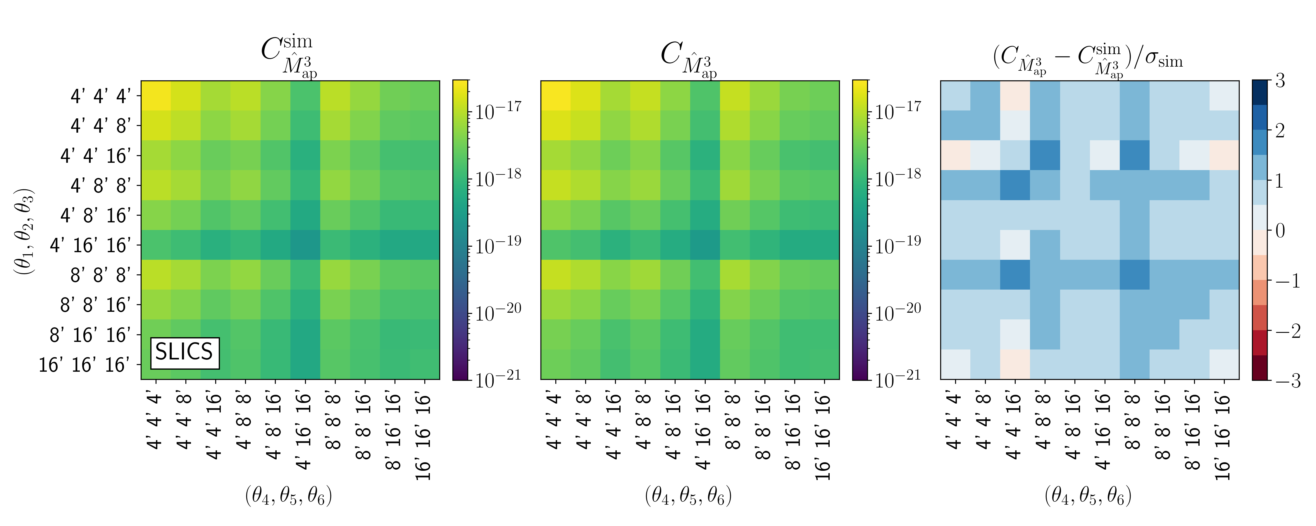
We estimate the covariance of M^ap3\hat{M}_{\mathrm{ap}}^{3} in three ways from the validation data. In the first method, we measure the aperture statistics ⟨Map3⟩\expectationvalue{\Map^3} on all simulation realisations using FFT and then use the sample covariance as an estimate. In the second method, we measure the third-order shear correlation functions Γi\Gamma_{i} and convert them to estimates of ⟨Map3⟩\expectationvalue{\Map^3} for all simulation realisations. Finally, in the third method, we measure the aperture mass correlation functions and convert them to the terms TP​P​P,1T_{PPP,1} to TP6T_{P_{6}} (see Sect. 3.3).

We choose the same aperture filter scales as used in 15 between 4​′ and 32​′. There, we showed that ⟨Map3⟩\expectationvalue{\Map^3} at these scales contains cosmological information that is complementary to the information content of second-order statistics. Our choice of scales also is impacted by two practical concerns: At aperture filters larger than 32​′ the signal-to-noise for ⟨Map3⟩\expectationvalue{\Map^3} becomes small, and at scales smaller than 4​′, the ⟨Map3⟩\expectationvalue{\Map^3}-model disagrees with simulations (see Fig. 8 in 15).

5.2.1 Using FFT

The measurement of ⟨Map3⟩\expectationvalue{\Map^3} in the simulations uses the same setup as the method described in 15. We will summarise it here shortly. For the flat GRFs and the SLICS, we measure CM^ap3C_{\hat{M}_{\mathrm{ap}}^{3}} in the shear maps in three steps.

At first, we measure Mapi​(ϑ,θ){M_{\mathrm{ap}}}_{i}(\bm{\vartheta},\theta) for each realisation ii, using scale radii θ∈{4​′,8​′,16​′}\theta\in\{$$,$$,$$\} for the SLICS and θ∈{4​′,8​′,16​′,32​′}\theta\in\{$$,$$,$$,$$\} for the GRFs. We use Eq. (7), which defines aperture mass maps as convolutions of the filter function QQ and the tangential shear. We evaluate these convolutions using the convolution theorem, by first Fourier transforming QQ and γt\gamma_{\mathrm{t}} with FFT, then multiplying them and inverse Fourier transforming the product. To remove edge effects, we cut off a border of 4 times the largest aperture radius, that is 4×32​′=128​′4\times$$=$$ for the GRFs and 4×16​′=64​′4\times$$=$$ for the SLICS, from each side of the Mapi{M_{\mathrm{ap}}}_{i}-maps. This large cut-off is needed because our filter function QθQ_{\theta} has infinite support and is significantly non-zero even for ϑ>θ\vartheta>\theta. The filter contains 99.9%99.9\% of its power within 4​θ4\theta, so with the cut-off, boundary effects are negligible. The resulting Mapi{M_{\mathrm{ap}}}_{i}-maps have side lengths ϑmax∈{5.73​°,10.73​°,15.73​°}\vartheta_{\mathrm{max}}\in\{$$,$$,$$\} for the GRFs and 7.87​° for the SLICS.

Then, we estimate ⟨Map3⟩i\expectationvalue{\Map^3}_{i} for each realisation ii. For this, we multiply Mapi​(ϑ,θ1){M_{\mathrm{ap}}}_{i}(\bm{\vartheta},\theta_{1}), Mapi​(ϑ,θ2){M_{\mathrm{ap}}}_{i}(\bm{\vartheta},\theta_{2}), and Mapi​(ϑ,θ3){M_{\mathrm{ap}}}_{i}(\bm{\vartheta},\theta_{3}) and then average over ϑ\bm{\vartheta}. Finally, we estimate the measured covariance CM^ap3measC^{\mathrm{meas}}_{\hat{M}_{\mathrm{ap}}^{3}} with

CM^ap3sim​(Θ1,Θ2)\displaystyle C^{\mathrm{sim}}_{\hat{M}_{\mathrm{ap}}^{3}}(\Theta_{1},\Theta_{2}) =1N−1​∑i=1N⟨Map3⟩i​(θ1,θ2,θ3)​⟨Map3⟩i​(θ4,θ5,θ6)\displaystyle=\frac{1}{N-1}\sum_{i=1}^{N}\expectationvalue{\Map^3}_{i}(\theta_{1},\theta_{2},\theta_{3})\expectationvalue{\Map^3}_{i}(\theta_{4},\theta_{5},\theta_{6}) (57)
−1N⁡(N−1)∑i=1N⟨Map3⟩i(θ1,θ2,θ3)∑j=1N⟨Map3⟩j(θ4,θ5,θ6).\displaystyle\quad-\frac{1}{N(N-1)}\sum_{i=1}^{N}\expectationvalue{\Map^3}_{i}(\theta_{1},\theta_{2},\theta_{3})\sum_{j=1}^{N}\expectationvalue{\Map^3}_{j}(\theta_{4},\theta_{5},\theta_{6})\;.

For the curved-sky T17 convergence maps, we smooth the maps with the healpy function smoothing with a beam window function determined by the corresponding UθU_{\theta} filter for the same aperture radii as for the GRFs, which are θ∈{4​′,8​′,16​′,32​′}\theta\in\{$$,$$,$$,$$\}. Each filter yields a full-sky aperture mass map Mapi{M_{\mathrm{ap}}}_{i}, from which we extracted 18 tiles that are not adjacent. This gives in total 1944 almost independent realisations.

We compute uncertainty estimates with bootstrapping for both the SLICS and the T17 covariances from FFT. For this, we generate 10 00010\,000 vectors containing NrealN_{\mathrm{real}} randomly drawn integers between 1 and NrealN_{\mathrm{real}} where NrealN_{\mathrm{real}} is the number of realisations (924 for the SLICS and 1944 for the T17). The vectors can explicitly contain the same integer multiple times. For each vector, we take the ⟨Map3⟩i\expectationvalue{\Map^3}_{i} for which ii is an element in the vector and use it to calculate a sample covariance with Eq. (57). In this way, we obtain 10 00010\,000 covariance estimates. We take the standard deviation of these estimates as uncertainty for the CM^ap3simC_{\hat{M}_{\mathrm{ap}}^{3}}^{\mathrm{sim}}.

5.2.2 Using third-order shear correlation functions

As mentioned in Sect. 2, ⟨Map3⟩\expectationvalue{\Map^3} is related to the natural components Γi\Gamma_{i} of the third-order shear correlation function (15, see also Section 5.3 in). Therefore, we can estimate the ⟨Map3⟩i\expectationvalue{\Map^3}_{i} of each simulation realisation ii by first measuring the Γi\Gamma_{i} and then converting them to ⟨Map3⟩i\expectationvalue{\Map^3}_{i}, following Equations (69) and (71) of Schneider et al. 2005. The covariance of M^ap3\hat{M}_{\mathrm{ap}}^{3} can then be estimated as the sample variance of the ⟨Map3⟩i\expectationvalue{\Map^3}_{i}, using Eq. (57).

We expect the covariance estimate from this approach to be smaller than the estimate from the FFT-based method described in the previous subsection. This is because, here, we do not cut off the border of the survey area. Consequently, more shear information is used to estimate ⟨Map3⟩\expectationvalue{\Map^3}, leading to a smaller covariance.

The measurement of the Γi\Gamma_{i} is very time-intensive. Therefore, we restrict this approach to the SLICS data, where we measure the Γi\Gamma_{i} using treecorr (Jarvis et al. 2004). We use ten bins each for the triangle parameters u,v,u,v, and rr with rr between 0.1​′ and 120​′. As shown in 15, binning the Γi\Gamma_{i} in this way yields accurate ⟨Map3⟩\expectationvalue{\Map^3} for scale radii between 4​′ and 16​′.

5.2.3 Using aperture mass correlation functions

As shown in Sect. 3.3, the individual terms of the covariance can be estimated from the aperture mass correlation functions, which we use to validate the analytic expressions.

For this, we measure the aperture mass maps Mapi​(ϑ,θ){M_{\mathrm{ap}}}_{i}(\bm{\vartheta},\theta) according to Sect. 5.2.1. From these maps, we first calculate the Mapi​(ϑ,θ1)​Mapi​(ϑ,θ2){M_{\mathrm{ap}}}_{i}(\bm{\vartheta},\theta_{1}){M_{\mathrm{ap}}}_{i}(\bm{\vartheta},\theta_{2}) and Mapi​(ϑ,θ1)​Mapi​(ϑ,θ2)​Mapi​(ϑ,θ3){M_{\mathrm{ap}}}_{i}(\bm{\vartheta},\theta_{1}){M_{\mathrm{ap}}}_{i}(\bm{\vartheta},\theta_{2}){M_{\mathrm{ap}}}_{i}(\bm{\vartheta},\theta_{3}) by multiplying the aperture mass maps for different filter radii. Then, we estimate the correlation functions Map2,1​(θ1,θ2,η)M_{\mathrm{ap}}^{2,1}(\theta_{1};\theta_{2};\eta), Map3,1​(θ1,θ2,θ3,η)M_{\mathrm{ap}}^{3,1}(\theta_{1},\theta_{2};\theta_{3};\eta), Map4,3​(θ1,θ2,θ3,θ4,η)M_{\mathrm{ap}}^{4,3}(\theta_{1},\theta_{2},\theta_{3};\theta_{4};\eta), and Map4,2​(θ1,θ2,θ3,θ4,η)M_{\mathrm{ap}}^{4,2}(\theta_{1},\theta_{2};\theta_{3},\theta_{4};\eta) by correlating the relevant aperture mass maps: We first extend the fields Mapi​(ϑ,θ){M_{\mathrm{ap}}}_{i}(\bm{\vartheta},\theta) using zero-padding, meaning that we add pixel grids containing only zeros to the boundary of the map. Doing this, Mapi​(ϑ,θ){M_{\mathrm{ap}}}_{i}(\bm{\vartheta},\theta) becomes WA​(ϑ)​Mapi​(ϑ,θ)W_{A}(\bm{\vartheta})\,{M_{\mathrm{ap}}}_{i}(\bm{\vartheta},\theta). The correlation between two aperture mass maps then yields

∫Adϑ​WA​(ϑ)​Mapi​(ϑ,θ1)​WA​(ϑ+η)​Mapi​(ϑ+η,θ2)=E⁡(η)​Map2​(θ1,θ2,η).\int_{A}\differential[]\vartheta\;W_{A}(\bm{\vartheta})\,{M_{\mathrm{ap}}}_{i}(\bm{\vartheta},\theta_{1})\,W_{A}(\bm{\vartheta}+\mathbf{\eta})\,{M_{\mathrm{ap}}}_{i}(\bm{\vartheta}+\mathbf{\eta},\theta_{2})=E(\mathbf{\eta})\,M_{\mathrm{ap}}^{2}(\theta_{1},\theta_{2};\mathbf{\eta})\;. (58)

We perform this correlation using the correlate2D function from scipy. Finally, we calculate the terms TP​P​P,1T_{PPP,1} to TP6T_{P_{6}} with the expressions in Sect. 3.3.

Our method to measure the correlation function uses the flat-sky approximation, so we did not apply it to the T17 simulations. Furthermore, the correlation function estimation of the terms TP​P​P,2T_{PPP,2} and TP​T,2T_{PT,2} is strongly affected by noise, which is why we only use it for the SLICS without shape noise.

5.3 Results

5.3.1 Gaussian random fields

We compare the covariance for ⟨Map3⟩\expectationvalue{\Map^3} measured in the simulated GRFs with the analytical expression TP​P​P,1+TP​P​P,2T_{PPP,1}+T_{PPP,2} and the large-field approximation TP​P​P,1∞T_{PPP,1}^{\infty} in Fig. 4. For the GRFs, all terms containing the bi-, tri-, or pentaspectrum vanish, so the middle column gives the full analytical prediction for the covariance. We see that, as expected, both simulated and analytical covariance decrease with increasing survey size. The full analytic covariance shows similar values to the simulated covariance for all combinations of aperture radii. The large-field approximation agrees only on and near the diagonal with the simulation and is much smaller for elements far from the diagonal.

Refer to caption

Figure 4: CM^ap3C_{\hat{M}_{\mathrm{ap}}^{3}} for the GRF, each row is showing a different field size. In the left column are the measured CM^ap3C_{\hat{M}_{\mathrm{ap}}^{3}} from the simulated GRF. The middle column shows the model prediction, including the finite-field term TP​P​P,2T_{PPP,2}. The covariances under the large-field approximation, for which TP​P​P,2T_{PPP,2} vanishes, are in the right column.

This observation is quantified in Fig. 5, where we show the fractional differences between the simulated and analytically calculated covariances. The full analytical expression shows deviations of less than 30% to the simulation, while the large-field approximation is almost a factor of two too small for the non-diagonal elements. While the deviations decrease with field size, they are still significant for the largest side length of 15.73​°. Consequently, neglecting TP​P​P,2T_{PPP,2} is inappropriate, even for surveys of a size of (15.73​°)2=247.43​deg2($$)^{2}=247.43\,\mathrm{deg}^{2}.

Refer to caption

Figure 5: Fractional differences of the model covariance to the measured CM^ap3C_{\hat{M}_{\mathrm{ap}}^{3}} for the GRF, each row showing a different field size. In the left column are the fractional differences between the full analytic model and the simulated GRF. The middle column shows the difference between the large-field approximation, neglecting the finite field term, and the simulated covariance. In the right column, the difference of the model using the large-field approximation for TP​P​P,1T_{PPP,1}, but keeping TP​P​P,2T_{PPP,2} as it is, is shown.

The remaining disagreement between the full analytic covariance model and the simulations can be explained by the discreteness of the shear maps. Due to the finite pixel number, the shear maps contain only modes which are ℓ=2​π​i2+j2/ϑmax′\ell=2\pi\sqrt{i^{2}+j^{2}}/\vartheta^{\prime}_{\mathrm{max}}, where ii and jj are integers between 0 and Npix/2N_{\mathrm{pix}}/2, where NpixN_{\mathrm{pix}} is the pixel number and ϑmax′\vartheta^{\prime}_{\mathrm{max}} is the side length of the shear maps (before boundary cut-off). Therefore, while the model assumes a smooth power spectrum P⁡(ℓ)P(\ell), the actual power spectrum of the GRFs is

PGRF​(ℓ)=(2​πϑmax′)2​∑i=1Npix/2∑j=1Npix/2P⁡(2​π​i2+j2ϑmax′)​δD​(ℓ1−2​π​iϑmax′)​δD​(ℓ2−2​π​jϑmax′),P^{\mathrm{GRF}}(\bm{\ell})=\left(\frac{2\pi}{\vartheta^{\prime}_{\mathrm{max}}}\right)^{2}\,\sum_{i=1}^{N_{\mathrm{pix}}/2}\sum_{j=1}^{N_{\mathrm{pix}}/2}P\left(\frac{2\pi\sqrt{i^{2}+j^{2}}}{\vartheta^{\prime}_{\mathrm{max}}}\right)\,\delta_{\mathrm{D}}\left(\ell_{1}-\frac{2\pi i}{\vartheta^{\prime}_{\mathrm{max}}}\right)\,\delta_{\mathrm{D}}\left(\ell_{2}-\frac{2\pi j}{\vartheta^{\prime}_{\mathrm{max}}}\right)\;, (59)

with ℓ=(ℓ1,ℓ2)\bm{\ell}=(\ell_{1},\ell_{2}). Due to the large pixel number, it is not feasible to directly calculate TP​P​P,1T_{PPP,1} and TP​P​P,2T_{PPP,2} for this power spectrum. However, using PGRFP^{\mathrm{GRF}} is similar to assuming that PP is zero for ℓ\ell outside of [ℓmin,ℓmax][\ell_{\mathrm{min}},\ell_{\mathrm{max}}], with ℓmin=2​π/ϑmax′\ell_{\mathrm{min}}=2\pi/\vartheta^{\prime}_{\mathrm{max}}, and ℓmax=π​Npix/ϑmax′\ell_{\mathrm{max}}=\pi\,N_{\mathrm{pix}}/\vartheta^{\prime}_{\mathrm{max}}. This is the same as increasing the lower and decreasing the upper integration boundary for the ℓ\ell-integrals in TP​P​P,1T_{PPP,1} and TP​P​P,2T_{PPP,2}. We show the impact of these integration borders in Fig. 6. The upper boundary ℓmax\ell_{\mathrm{max}}, and consequently the pixel number, has only a small impact on the model covariance. This is because the aperture filters u^\hat{u} decrease with ℓ\ell and are already small at ℓ≃ℓmax\ell\simeq\ell_{\mathrm{max}}. The lower boundary ℓmin\ell_{\mathrm{min}} has a stronger impact. By increasing the lower integration border to ℓmin\ell_{\mathrm{min}}, we decrease the model covariance. This decrease significantly improves the agreement between the simulated GRFs and the model.

Refer to caption
Figure 6: Fractional differences between covariance model and estimate from GRFs with ϑmax=5.78​°\vartheta_{\mathrm{max}}=$$ for different choices of the boundaries of the ℓ\ell-integrals. Left: Fiducial calculation of model, where P⁡(ℓ)P(\ell) is used for all ℓ\ell. Middle: ℓ\ell-modes larger than ℓmax\ell_{\mathrm{max}} are cut-off. This removes modes not present in the simulation due to the finite pixel size. Right: ℓ\ell-modes smaller than ℓmin\ell_{\mathrm{min}} are cut-off. This removes modes not present in the simulation due to the finite field size.

As the field size (and ϑmax′\vartheta^{\prime}_{\mathrm{max}}) increases, ℓmin\ell_{\mathrm{min}} decreases so that smaller ℓ\ell-modes are included in the GRFs. Therefore, the difference between the model, evaluated for all ℓ\ell, and the covariance from the GRFs shrinks with increasing field size, as seen in the right column of Fig. 5.

We also show in Fig. 5 the fractional difference between TP​P​P,1∞+TP​P​P,2T_{PPP,1}^{\infty}+T_{PPP,2} and the simulated covariance. This approximated analytic expression shows a similar level of agreement with the simulated covariance as the full expression. The cause of this good agreement is the similarity between TP​P​P,1T_{PPP,1} and TP​P​P,1∞T_{PPP,1}^{\infty}, shown in Fig. 7. Even for the smallest field size with side length ϑmax=5.73​°\vartheta_{\mathrm{max}}=$$, most elements of TP​P​P,1T_{PPP,1} and TP​P​P,1∞T_{PPP,1}^{\infty} differ by less than 5%, with stronger deviations mostly at very large aperture radii (32​′) or very small aperture radii (4​′). For the largest field, all elements agree at better than 15%.

Refer to caption
Figure 7: Fractional differences of TP​P​P,1T_{PPP,1} with and without large-field approximation for different field sizes

The agreement between TP​P​P,1T_{PPP,1} and TP​P​P,1∞T_{PPP,1}^{\infty} encourages a practical simplification, which is substituting TP​P​P,1T_{PPP,1} by the large-field approximation. This significantly simplifies the calculation: Equation (44) to obtain TP​P​P,1∞T_{PPP,1}^{\infty} contains only three integrals, while Eq. (20) for TP​P​P,1T_{PPP,1} contains six integrals, two of which involve oscillating functions. Consequently, the numerical integration for TP​P​P,1∞T_{PPP,1}^{\infty} is much simpler and faster.

The finite field effect, which gives rise to TP​P​P,2T_{PPP,2}, can be important for covariance estimates derived from simulations. Such estimates are sometimes performed on simulations with a smaller area than the survey to which the covariance is applied. To account for the different areas, the covariances are rescaled by a factor Asim/AsurveyA_{\mathrm{sim}}/A_{\mathrm{survey}}, where AsimA_{\mathrm{sim}} and AsurveyA_{\mathrm{survey}} are the simulation and survey areas, respectively. This rescaling assumes that the covariance is inversely proportional to the survey area, which is only true under the large-field approximation. While TP​P​P,1∞T_{PPP,1}^{\infty} indeed scales with the inverse survey area, TP​P​P,2T_{PPP,2} decreases faster, as shown in Sect. 3.4. We demonstrate the failure of the rescaling approach in Fig. 8, where we show the fractional difference between the covariance for the simulated GRF with a side length of 15.73​° and the analytical estimate for the side length 5.73​°, rescaled by the factor (5.73/15.73)2(5.73/15.73)^{2}. The rescaled covariance is too large by a factor of up to 4.7.

Refer to caption
Figure 8: Fractional difference of model covariance, rescaled from a field size of 5.73​°2$$^{2} to 15.73​°2$$^{2} to the covariance from a simulated GRF of size 15.73​°2$$^{2}. The rescaling is performed under the assumption that the covariance scales inversely proportional to the survey area, which is not true for the finite field term TP​P​P,2T_{PPP,2}.

5.3.2 NN-body simulations

We now compare the full analytic CM^ap3C_{\hat{M}_{\mathrm{ap}}^{3}}, including the non-Gaussian terms, to the covariances from the NN-body simulations. Figure 9 compares the CM^ap3C_{\hat{M}_{\mathrm{ap}}^{3}} and CM^ap3simC_{\hat{M}_{\mathrm{ap}}^{3}}^{\mathrm{sim}} for the SLICS and the T17 simulations. For the SLICS, we see deviations of 1 to 2 times the simulation uncertainty, with the model being larger than the simulated covariance at most scales. These deviations could indicate that the power-, tri-, and pentaspectrum of the SLICS do not correspond to the model polyspectra. This could be caused by the finite resolution and smoothing in the simulations, the need for additional halo terms for the tri- and pentaspectrum in the model, or the general inaccuracy of the halo model. However, for the T17, we generally see a better agreement between simulation and model. Most elements agree within the simulation accuracy, with a few elements outside the 2​σ2\sigma range.

Refer to caption
Refer to caption
Figure 9: Comparison of measured and modelled covariance for the SLICS (top) and T17 simulations (bottom). Left are the measured covariance, middle are the model predictions; right are the differences between model and simulation, normalised by the simulation bootstrap error.

We compare the diagonals of the individual terms of the analytic covariance in Fig. 10. We see that for both the SLICS and T17 setup, the non-Gaussian terms are dominant. For the SLICS, TP6T_{P_{6}} dominates on the scales considered here, whereas for the T17, the first Gaussian term TP​P​P,1T_{PPP,1} is of a similar magnitude as TP6T_{P_{6}}. This difference is caused by the different levels of shape noise in the two simulations. For the SLICS, we use a Stage-IV-like setup, where the galaxy number density is ng=30​arcmin−2n_{\mathrm{g}}=30\,\mathrm{arcmin}^{-2}, while the T17 use the KiDS-like number density of ng=6.17​arcmin−2n_{\mathrm{g}}=6.17\,\mathrm{arcmin}^{-2}. Therefore, the Gaussian covariance term for the T17 has a larger impact than for the SLICS. The relative importance of the Gaussian and non-Gaussian terms is also related to the considered aperture radii. For larger scales, the importance of the Gaussian terms increases, while the contribution of the pentaspectrum-term decreases, as shown in Fig. 11 for the SLICS setup and aperture radii between 16​′ and 64​′. However, we stress that we consider these large scales suboptimal for cosmological analyses with ⟨Map3⟩\expectationvalue{\Map^3} since, as mentioned in Sect. 5.2, the matter field is more Gaussian and the signal-to-noise of third-order statistics is small.

Refer to caption
Refer to caption
Figure 10: Diagonal of CM^ap3C_{\hat{M}_{\mathrm{ap}}^{3}} and the individual covariance terms for the SLICS (left) and the T17 (right). The measurement from the simulation is shown as a red dashed line, while the full modelled CM^ap3C_{\hat{M}_{\mathrm{ap}}^{3}} is the bold black line. The other lines show individual terms. Error bars on the simulated covariances originate from bootstrapping
Refer to caption
Figure 11: Model predictions for the individual covariance terms for the SLICS-like setup.

As mentioned before, we can also directly measure the individual covariance terms and compare them to the analytic prediction in Fig. 13 using aperture mass correlation functions. Unfortunately, measuring the finite-field terms TP​P​P,2T_{PPP,2} and TP​T,2T_{PT,2} is challenging: In Eqs. (36) and (39), one can see that, when neglecting the function EA​(η)E_{A}(\mathbf{\eta}), the integral over the correlation function is, by definition, zero. So the only part that leads to TP​P​P,2T_{PPP,2} and TP​T,2T_{PT,2} being non-zero is multiplication with the slowly varying function EA​(η)E_{A}(\mathbf{\eta}). This amplifies the effect of noise in the measured correlation function. Thus, the measurements of TP​P​P,2T_{PPP,2} and TP​T,2T_{PT,2} are very sensitive to the noise level, and we can only perform them in the SLICS without shape noise. We note that the source galaxies in this data set are all situated at redshift z=1z=1 and do not follow the same redshift distribution as the data used for Fig. 10. The measured and modelled covariance terms show similar dependencies on the aperture scale radii. The model for the dominating term TP6T_{P_{6}} agrees within a few per cent with the measurement. For TP​P​P,1T_{PPP,1}, TP​P​P,2T_{PPP,2}, and TP​T,2T_{PT,2}, though, the model underpredicts the measurements. This difference is likely due to differences between the model polyspectra and the actual polyspectra of the simulation. Since our trispectrum model contains only the 1-halo term, we do not expect a perfect match between the modelled TP​T,1T_{PT,1} and TP​T,2T_{PT,2} and the measurement. Furthermore, the BiHalofit bispectrum model only agrees with the data at the 10%10\% level, (15, compare to Appendix A of), so deviations at the 20%20\% level are expected for TB​BT_{BB}, which depends on the square of the bispectrum.

Refer to caption
Figure 12: Comparison of individual covariance terms modelled (solid) and measured (dashed) in the SLICS without shape noise and with all sources at redshift 1

.

Refer to caption
Figure 13: Ratio of two-halo contribution TP6,2​hT_{P_{6},\mathrm{2h}} to full TP6T_{P_{6}} term for various field sizes with T17 cosmology. The blue line corresponds to the KiDS1000-like field size.

The term TP6,2​hT_{P_{6},\mathrm{2h}} gives a significant contribution to TP6T_{P_{6}}. We show this in Fig. 13, where the blue line shows the diagonal of the ratio between TP6,2​hT_{P_{6},\mathrm{2h}} and TP6∞+TP6,2​hT_{P_{6}}^{\infty}+T_{P_{6},\mathrm{2h}} for the T17 setup. The two-halo term is substantial for small apertures and the combinations of small and large apertures. The figure also shows the same ratio for larger field sizes. The importance of TP6,2​hT_{P_{6},\mathrm{2h}} decreases with field size. This is as expected, since TP6∞T_{P_{6}}^{\infty} scales with the inverse survey area, while TP6,2​hT_{P_{6},\mathrm{2h}} decreases faster.

Refer to caption
Figure 14: Covariance in SLICS, measured with shear correlation functions Γi\Gamma_{i} (black) and FFT (blue), as well as the model covariance for the full survey area of 10​°×10​°$$\times$$ (orange, dashed) and for the effective survey area of 7.87​°×7.87​°$$\times$$.

Finally, we compare the covariance estimated in the SLICS using the shear three-point correlation function Γi\Gamma_{i} to the FFT-based estimate in Fig. 14. We also show the model prediction for two different survey areas: either the entire survey area of 10​°×10​°$$\times$$ or the survey area of 7.87​°×7.87​°$$\times$$ after boundary removal. As expected, the FFT-based covariance estimate is larger than the Γi\Gamma_{i}-based estimate. This is a direct consequence of the boundary removal for the FFT - the effective survey area shrinks.

The Γi\Gamma_{i}-based covariance is itself larger than the full-survey model covariance. This is because, as mentioned before, estimates of ⟨Map3⟩\expectationvalue{\Map^3} for the whole survey area A′A^{\prime} require shear information outside of A′A^{\prime}. Consequently, unbiased estimates of ⟨Map3⟩\expectationvalue{\Map^3} on A′A^{\prime} contain more information than estimates of Γi\Gamma_{i}, which are restricted to A′A^{\prime}. Therefore, the covariance of the Γi\Gamma_{i}-based estimator lies in between the model covariance for the total area A′A^{\prime} and cut-off survey area AA. Since the Γi\Gamma_{i}-based estimator is required to analyse survey data, the covariance model gives an upper and lower bound to the expected survey constraints.

6 Influence of covariance terms on cosmological parameter estimation

We have shown in the previous section that the analytical covariance estimates agree with estimates from the simulations within 1–2 times the simulations’ statistical uncertainty. However, it is unclear whether this level of agreement is sufficient for a cosmological parameter analysis. To test this, in this section, we perform mock MCMC analyses using CM^ap3C_{\hat{M}_{\mathrm{ap}}^{3}} and CM^ap3simC_{\hat{M}_{\mathrm{ap}}^{3}}^{\mathrm{sim}}, and compare the resulting parameter constraints. We also test the impact of the individual covariance terms on the cosmological analysis.

6.1 Analysis setup

We perform mock cosmological analyses with the same setup as in 15. In this setup, we use the neural network emulator CosmoPower (Spurio Mancini et al. 2022) to quickly evaluate the ⟨Map3⟩\expectationvalue{\Map^3} model and sample the parameter likelihood. With the trained emulator, we evaluate the parameter likelihoods for different choices for the covariance: the estimate from the simulations, the full analytic expressions, and various combinations of the individual terms of CM^ap3C_{\hat{M}_{\mathrm{ap}}^{3}}. Since the ⟨Map3⟩\expectationvalue{\Map^3} are not sensitive to w0w_{0} and hh in a non-tomographic setting, we evaluate the likelihood for fixed w0=−1w_{0}=-1 and h=0.69h=0.69. For the T17 validation, we evaluated the ⟨Map3⟩\expectationvalue{\Map^3}-model at the aperture scale radii 4​′,8​′,16​′,$$,$$,$$, and 32​′, whereas for the SLICS setup, we used the aperture scale radii 4​′,8​′,$$,$$, and 16​′. The reference data vector is measured at the corresponding cosmology of the respective simulation.

6.2 Results

In the left panel of Fig. 15, we show the T17 results for the constraints on Ωm\Omega_{\mathrm{m}}, S8S_{8}, and σ8\sigma_{8}, while varying only Ωm\Omega_{\mathrm{m}} and S8S_{8}. In Table 1, we report the resulting marginalised parameter constraints together with the figure of merit (FoM) estimated as

FoM=1det⁡(C),\mathrm{FoM}=\frac{1}{\sqrt{\mathrm{det}(C)}}\,, (60)

where CC is the parameter covariance matrix resulting from the MCMC process. The T17 covariances are tailored to a KiDS-like survey area and shape noise. The constraints from the simulated and analytic covariance coincide. The FoM of Ωm\Omega_{\mathrm{m}}–S8S_{8} differs by less than 3%. Consequently, the analytic covariance is ideal for an unbiased cosmological analysis in our setup. We display in the right panel of Fig. 15 the comparison for the SLICS setup. The posteriors for both the simulated and modelled covariance matrix clearly agree. This supports the robustness of the modelled covariance for varying survey areas, shape noise and redshift distribution.

Refer to caption
Refer to caption
Figure 15: Parameter constraints, using either the covariance from the simulations (red) or the analytic model (black). Left are the constraints for a KiDS-1000-like survey, and right are the constraints for the SLICS setup, which uses a stage IV-like n⁡(z)n(z) and shape noise, but a small survey area of 7.87​°×7.87​°$$\times$$
Table 1: Overview of the marginalised MAP values and 68%68\% confidence intervals resulting from MCMC chains where Ωm\Omega_{\mathrm{m}}, S8S_{8} are varied and σ8=S8​0.3/Ωm\sigma_{8}=S_{8}\sqrt{0.3/\Omega_{\mathrm{m}}}. We fixed h=0.7h=0.7 and w0=−1w_{0}=-1.
MAP Ωm\Omega_{\mathrm{m}} σ8\sigma_{8} S8S_{8}
T17 0.272−0.065+0.1480.272^{+0.148}_{-0.065} 0.665−0.038+0.1730.665^{+0.173}_{-0.038} 0.798−0.029+0.0230.798^{+0.023}_{-0.029}
analytic model (all terms) 0.259−0.048+0.1660.259^{+0.166}_{-0.048} 0.661−0.035+0.1720.661^{+0.172}_{-0.035} 0.798−0.027+0.0230.798^{+0.023}_{-0.027}
analytic model (all terms, without 2-halo term) 0.260−0.047+0.1700.260^{+0.170}_{-0.047} 0.663−0.033+0.1660.663^{+0.166}_{-0.033} 0.798−0.021+0.0210.798^{+0.021}_{-0.021}
analytic model (neglecting finite-field terms) 0.271−0.061+0.1500.271^{+0.150}_{-0.061} 0.661−0.033+0.1710.661^{+0.171}_{-0.033} 0.797−0.025+0.0230.797^{+0.023}_{-0.025}
analytic model (only Gaussian) 0.271−0.052+0.1320.271^{+0.132}_{-0.052} 0.664−0.019+0.1640.664^{+0.164}_{-0.019} 0.795−0.013+0.0150.795^{+0.015}_{-0.013}
FoM Ωm\Omega_{\mathrm{m}}-σ8\sigma_{8} Ωm\Omega_{\mathrm{m}}-S8S_{8} σ8\sigma_{8}-S8S_{8}
T17 293 429 341
analytic model (all terms) 299 441 353
analytic model (all terms, without 2-halo term) 334 561 445
analytic model (neglecting finite-field terms) 321 482 388
analytic model (only Gaussian) 553 1216 966

In Fig. 16, we compare the parameter constraints obtained when using the total analytic covariance estimate, only the Gaussian terms TP​P​P,1T_{PPP,1} and TP​P​P,2T_{PPP,2}, when neglecting the finite-field terms TP​P​P,2T_{PPP,2} and TP​T,2T_{PT,2}, and when neglecting the term TP6,2​hT_{P_{6},\mathrm{2h}}. The results demonstrate the importance of the non-Gaussian covariance terms, as the FoM of Ωm\Omega_{\mathrm{m}}–S8S_{8} approximately triples if only the Gaussian terms are used (see Table 1). Consequently, for the application to a Stage III survey, non-Gaussian covariance terms for ⟨Map3⟩\expectationvalue{\Map^3} cannot be neglected.

For the KiDS-like survey area used here, the finite-field terms TP​P​P,2T_{PPP,2} and TP​T,2T_{PT,2} play a secondary role (see Table 1). The FoM of Ωm\Omega_{\mathrm{m}}-S8S_{8} increases by 12% if these terms are neglected. Consequently, depending on the desired accuracy of the modelled covariance, these terms could be neglected for a real parameter analysis. Since calculating TP​P​P,2T_{PPP,2} and TP​T,2T_{PT,2} for a real survey requires evaluating Eq. (22) for the true, most likely complicated, survey geometry, bypassing them could significantly decrease the computational complexity of the covariance calculation. Ignoring TP6,2​hT_{P_{6},\mathrm{2h}}, the 2-halo contribution to TP6T_{P_{6}}, has a stronger effect. Neglecting TP6,2​hT_{P_{6},\mathrm{2h}} increases the FoM of Ωm\Omega_{\mathrm{m}}-S8S_{8} by 27% and has a significant impact on the inferred constraints on the individual parameters.

Refer to caption
Figure 16: Parameter constraints for a KiDS-1000-like survey, using the full model covariance (black), neglecting the finite field terms (blue), neglecting the 2-halo contribution to TP6T_{P_{6}} (green) or using only the Gaussian covariance (orange). The FoMs of Ωm\Omega_{\mathrm{m}}-S8S_{8} are given in Table 1.

7 Discussion

In this work, we derived an analytic model for the covariance of the third-order aperture statistics ⟨Map3⟩\expectationvalue{\Map^3}. We make our modelling code publically available 33 3 https://github.com/sheydenreich/threepoint/releases.

We performed three tests for this analytic model. First, we compared the Gaussian part of the covariance to simulated GRFs. We found that all elements of the modelled covariance agree with the GRFs within 30%, with most elements agreeing better than 10% with the simulated data. Second, we compared the full model to two independent NN-body simulations, the SLICS and T17 simulations. These comparisons showed that the model agrees within 1–2 times the statistical uncertainty on the simulations with the simulated covariance estimates. Third, we compared the expected constraints from a KiDS-1000-like survey for the cosmological parameters Ωm\Omega_{\mathrm{m}} and S8S_{8} using the covariance from the T17 simulations and the analytic expression. The constraints were remarkably similar, with only a 3% deviation in the FoM on Ωm\Omega_{\mathrm{m}}-S8S_{8}. These three tests confirmed that our covariance model is sufficiently accurate for analysing a stage III survey.

Additionally, we found that all terms of the M^ap3\hat{M}_{\mathrm{ap}}^{3} covariance can be estimated by measuring aperture mass correlation functions. Using this approach, we compared the individual terms of the model to measurements in the SLICS and confirmed that the model agrees with the simulations.

In the derivation of the covariance model, we found terms that decrease faster than the inverse survey area and vanish entirely under the large-field approximation, which assumes an infinitely broad survey window function. These finite-field terms show a complex dependence on the survey geometry, while the other terms mainly scale with the inverse survey area. The finite field term TP​P​P,2T_{PPP,2} is already present in the Gaussian case. Comparing the model to GRFs showed that it is the dominating contribution for non-diagonal elements, and neglecting it leads to a severe bias. However, the effect of the finite-field term is small for the realistic covariances, including non-Gaussianity, as they are dominated by the pentaspectrum term TP6T_{P_{6}}. Ignoring the finite-field terms leads to an increment of only 12% in the FoM on Ωm\Omega_{\mathrm{m}}-S8S_{8}.

We showed that it is incorrect to derive the covariance for the real-space statistic M^ap3\hat{M}_{\mathrm{ap}}^{3} from a bispectrum covariance. Using an integral over a bispectrum covariance to model the covariance of M^ap3\hat{M}_{\mathrm{ap}}^{3} is only possible under the large-field approximation. However, in this case, one automatically neglects the finite-field terms.

We note that our covariance model assumes the flat-sky approximation. Nevertheless, the favourable comparison to the T17 simulation indicates that this assumption is valid at the relatively small scales considered here. This is not a surprising finding since we consider ⟨Map3⟩\expectationvalue{\Map^3} at small, sub-degree scales. At these small scales, the flat-sky approximation introduces no significant bias. Our model should therefore be applicable to actual observations.

Our covariance model is based on an estimator for ⟨Map3⟩\expectationvalue{\Map^3} that is easily applicable to simulations but should not be applied to realistic survey data, which include masks, because it requires a continuous convergence (or shear) map. Instead, one must use an estimator based on the third-order shear correlation functions. However, we have shown that our model can quantify the covariance of this estimator. The model covariance for the entire survey area gives a lower bound to the expected covariance, while the model covariance for a smaller effective area after boundary removal gives an upper bound. For a square survey with an area of 1000​deg21000\,\mathrm{deg}^{2} and a boundary cut-off of 4×16​′4\times$$, the upper bound is around 15%15\% above the lower bound, which gives relatively tight constraints on the true covariance. For even larger stage IV surveys, the bound will be tighter, as the boundary is a smaller fraction of the overall area.

In conclusion, we have presented and validated an analytic model for the covariance of third-order aperture statistics. Together with the analytical model for ⟨Map3⟩\expectationvalue{\Map^3} presented in 15, our covariance model paves the way for the cosmological analysis of third-order shear statistics of stage III and stage IV weak lensing surveys.

We have deliberately avoided the term super-sample covariance (SSC) to describe parts of CM^ap3C_{\hat{M}_{\mathrm{ap}}^{3}}. This term, originally devised for parts of the covariance of the power spectrum (Takada & Hu 2013), is used to describe covariance parts depending on ℓ\ell-modes larger than a given survey area. The term TP6,2​hT_{P_{6},\mathrm{2h}} corresponds to what is commonly called SSC for the bispectrum (Chan et al. 2018; Pyne & Joachimi 2021). However, as we will show in a forthcoming paper, the SSC can be defined as the difference between the exact form of a covariance and its large-field approximation. By this definition, the finite-field terms TP​P​P,2T_{PPP,2} and TP​T,2T_{PT,2} are also part of the SSC for M^ap3\hat{M}_{\mathrm{ap}}^{3}.

Acknowledgements.
Funded by the TRA Matter (University of Bonn) as part of the Excellence Strategy of the federal and state governments. This work has been supported by the Deutsche Forschungsgemeinschaft through the project SCHN 342/15-1 and DFG SCHN 342/13. PAB and SH acknowledge support from the German Academic Scholarship Foundation. We would like to thank Joachim Harnois-Déraps for making public the SLICS mock data, which can be found at http://slics.roe.ac.uk/. We thank Benjamin Joachimi, Susan Pyne, Lucas Porth and Niek Wielders for many helpful comments and discussions.

References

  • Abbott et al. (2022) Abbott, T. M. C., Aguena, M., Alarcon, A., et al. 2022, Phys. Rev. D, 105, 023520
  • Bartelmann (2010) Bartelmann, M. 2010, Classical and Quantum Gravity, 27, 233001
  • Bartelmann & Schneider (2001) Bartelmann, M. & Schneider, P. 2001, Phys. Rep, 340, 291
  • Burger et al. (2022) Burger, P. A., Friedrich, O., Harnois-Déraps, J., et al. 2022, arXiv:2208.02171
  • Chan et al. (2018) Chan, K. C., Moradinezhad Dizgah, A., & Noreña, J. 2018, Phys. Rev. D, 97, 043532
  • Cooray & Sheth (2002) Cooray, A. & Sheth, R. 2002, Phys. Rep, 372, 1
  • Crittenden et al. (2002) Crittenden, R. G., Natarajan, P., Pen, U.-L., & Theuns, T. 2002, ApJ, 568, 20
  • Friedrich et al. (2021) Friedrich, O., Andrade-Oliveira, F., Camacho, H., et al. 2021, MNRAS, 508, 3125
  • Friedrich et al. (2018) Friedrich, O., Gruen, D., DeRose, J., et al. 2018, Phys. Rev. D, 98, 023508
  • Giblin et al. (2021) Giblin, B., Heymans, C., Asgari, M., et al. 2021, A&A, 645, A105
  • Gruen et al. (2018) Gruen, D., Friedrich, O., Krause, E., et al. 2018, Phys. Rev. D, 98, 023507
  • Harnois-Déraps & van Waerbeke (2015) Harnois-Déraps, J. & van Waerbeke, L. 2015, MNRAS, 450, 2857
  • Heydenreich et al. (2022a) Heydenreich, S., Brück, B., Burger, P., et al. 2022a, A&A, 667, A125
  • Heydenreich et al. (2021) Heydenreich, S., Brück, B., & Harnois-Déraps, J. 2021, A&A, 648, A74
  • Heydenreich et al. (2022b) Heydenreich, S., Linke, L., Burger, P., & Schneider, P. 2022b, arXiv:2208.11686
  • Heydenreich et al. (2020) Heydenreich, S., Schneider, P., Hildebrandt, H., et al. 2020, A&A, 634, A104
  • Heymans et al. (2021) Heymans, C., Tröster, T., Asgari, M., et al. 2021, A&A, 646, A140
  • Hikage et al. (2019) Hikage, C., Oguri, M., Hamana, T., et al. 2019, PASJ, 71, 43
  • Hildebrandt et al. (2021) Hildebrandt, H., van den Busch, J. L., Wright, A. H., et al. 2021, A&A, 647, A124
  • Hoekstra & Jain (2008) Hoekstra, H. & Jain, B. 2008, Annual Review of Nuclear and Particle Science, 58, 99
  • Jarvis et al. (2004) Jarvis, M., Bernstein, G., & Jain, B. 2004, MNRAS, 352, 338
  • Joachimi et al. (2021) Joachimi, B., Lin, C. A., Asgari, M., et al. 2021, A&A, 646, A129
  • Joachimi et al. (2008) Joachimi, B., Schneider, P., & Eifler, T. 2008, A&A, 477, 43
  • Joachimi et al. (2009) Joachimi, B., Shi, X., & Schneider, P. 2009, A&A, 508, 1193
  • Kacprzak et al. (2016) Kacprzak, T., Kirk, D., Friedrich, O., et al. 2016, MNRAS, 463, 3653
  • Kaiser & Jaffe (1997) Kaiser, N. & Jaffe, A. 1997, ApJ, 484, 545
  • Kayo et al. (2013) Kayo, I., Takada, M., & Jain, B. 2013, MNRAS, 429, 344
  • Kilbinger & Schneider (2005) Kilbinger, M. & Schneider, P. 2005, A&A, 442, 69
  • Kuijken et al. (2015) Kuijken, K., Heymans, C., Hildebrandt, H., et al. 2015, MNRAS, 454, 3500
  • Martinet et al. (2021) Martinet, N., Harnois-Déraps, J., Jullo, E., & Schneider, P. 2021, A&A, 646, A62
  • Petri (2016) Petri, A. 2016, Astronomy and Computing, 17, 73
  • Pyne & Joachimi (2021) Pyne, S. & Joachimi, B. 2021, MNRAS, 503, 2300
  • Schneider (1996) Schneider, P. 1996, MNRAS, 283, 837
  • Schneider et al. (2005) Schneider, P., Kilbinger, M., & Lombardi, M. 2005, A&A, 431, 9
  • Schneider & Lombardi (2003) Schneider, P. & Lombardi, M. 2003, A&A, 397, 809
  • Schneider et al. (1998) Schneider, P., van Waerbeke, L., Jain, B., & Kruse, G. 1998, MNRAS, 296, 873
  • Secco et al. (2022) Secco, L. F., Jarvis, M., Jain, B., et al. 2022, Phys. Rev. D, 105, 103537
  • Seitz & Schneider (1996) Seitz, S. & Schneider, P. 1996, A&A, 305, 383
  • Sheth & Tormen (1999) Sheth, R. K. & Tormen, G. 1999, MNRAS, 308, 119
  • Springel et al. (2001) Springel, V., Yoshida, N., & White, S. D. M. 2001, Nature, 6, 79
  • Spurio Mancini et al. (2022) Spurio Mancini, A., Piras, D., Alsing, J., Joachimi, B., & Hobson, M. P. 2022, MNRAS, 511, 1771
  • Takada & Hu (2013) Takada, M. & Hu, W. 2013, Phys. Rev. D, 87, 123504
  • Takada & Jain (2004) Takada, M. & Jain, B. 2004, MNRAS, 348, 897
  • Takahashi et al. (2017) Takahashi, R., Hamana, T., Shirasaki, M., et al. 2017, ApJ, 850, 24
  • Takahashi et al. (2020) Takahashi, R., Nishimichi, T., Namikawa, T., et al. 2020, ApJ, 895, 113
  • Takahashi et al. (2012) Takahashi, R., Sato, M., Nishimichi, T., Taruya, A., & Oguri, M. 2012, ApJ, 761, 152
  • Troxel & Ishak (2012) Troxel, M. A. & Ishak, M. 2012, MNRAS, 419, 1804
  • van Waerbeke (2000) van Waerbeke, L. 2000, MNRAS, 313, 524
  • Zürcher et al. (2021) Zürcher, D., Fluri, J., Sgier, R., Kacprzak, T., & Refregier, A. 2021, J. Cosmology Astropart. Phys., 2021, 028

Appendix A List of all permutations for covariance terms

In Table 2, we list all permutations of aperture scale radii for the terms TP​P​P,1T_{PPP,1} to TP​T,2T_{PT,2} from Sect. 3. The first permutation corresponds to the expressions in Sect. 3. The vertical dashes separate groups of scale radii, in which the terms are symmetric. These symmetries can be easily seen in the expressions in terms of the aperture mass correlation functions in Sect. 3.3.

Table 2: Permutations of aperture scale radii for covariance terms.
Term permutations Term permutations Term permutations
TP​P​P,1T_{PPP,1} θ1​θ4​|θ2​θ5|​θ3​θ6\theta_{1}\theta_{4}|\theta_{2}\theta_{5}|\theta_{3}\theta_{6} TB​BT_{BB} θ2​θ3|θ4​|θ5​θ6|​θ1\theta_{2}\theta_{3}|\theta_{4}|\theta_{5}\theta_{6}|\theta_{1} TP​T,1T_{PT,1} θ1​θ4​|θ2​θ3|​θ5​θ6\theta_{1}\theta_{4}|\theta_{2}\theta_{3}|\theta_{5}\theta_{6}
θ1​θ4​|θ2​θ6|​θ3​θ5\theta_{1}\theta_{4}|\theta_{2}\theta_{6}|\theta_{3}\theta_{5} θ2​θ3|θ5​|θ4​θ6|​θ1\theta_{2}\theta_{3}|\theta_{5}|\theta_{4}\theta_{6}|\theta_{1} θ1​θ5​|θ2​θ3|​θ4​θ6\theta_{1}\theta_{5}|\theta_{2}\theta_{3}|\theta_{4}\theta_{6}
θ1​θ5​|θ2​θ4|​θ3​θ6\theta_{1}\theta_{5}|\theta_{2}\theta_{4}|\theta_{3}\theta_{6} θ2​θ3|θ6​|θ4​θ5|​θ1\theta_{2}\theta_{3}|\theta_{6}|\theta_{4}\theta_{5}|\theta_{1} θ1​θ6​|θ2​θ3|​θ4​θ5\theta_{1}\theta_{6}|\theta_{2}\theta_{3}|\theta_{4}\theta_{5}
θ1​θ5​|θ2​θ6|​θ3​θ4\theta_{1}\theta_{5}|\theta_{2}\theta_{6}|\theta_{3}\theta_{4} θ1​θ3|θ4​|θ5​θ6|​θ2\theta_{1}\theta_{3}|\theta_{4}|\theta_{5}\theta_{6}|\theta_{2} θ2​θ4​|θ1​θ3|​θ5​θ6\theta_{2}\theta_{4}|\theta_{1}\theta_{3}|\theta_{5}\theta_{6}
θ1​θ6​|θ2​θ4|​θ3​θ5\theta_{1}\theta_{6}|\theta_{2}\theta_{4}|\theta_{3}\theta_{5} θ1​θ3|θ5​|θ4​θ6|​θ2\theta_{1}\theta_{3}|\theta_{5}|\theta_{4}\theta_{6}|\theta_{2} θ2​θ5​|θ1​θ3|​θ4​θ6\theta_{2}\theta_{5}|\theta_{1}\theta_{3}|\theta_{4}\theta_{6}
θ1​θ6​|θ2​θ5|​θ3​θ4\theta_{1}\theta_{6}|\theta_{2}\theta_{5}|\theta_{3}\theta_{4} θ1​θ3|θ6​|θ4​θ5|​θ2\theta_{1}\theta_{3}|\theta_{6}|\theta_{4}\theta_{5}|\theta_{2} θ2​θ6​|θ1​θ3|​θ4​θ5\theta_{2}\theta_{6}|\theta_{1}\theta_{3}|\theta_{4}\theta_{5}
TP​P​P,2T_{PPP,2} θ1​θ2​|θ3​θ4|​θ5​θ6\theta_{1}\theta_{2}|\theta_{3}\theta_{4}|\theta_{5}\theta_{6} θ1​θ2|θ4​|θ5​θ6|​θ3\theta_{1}\theta_{2}|\theta_{4}|\theta_{5}\theta_{6}|\theta_{3} θ3​θ4​|θ1​θ2|​θ5​θ6\theta_{3}\theta_{4}|\theta_{1}\theta_{2}|\theta_{5}\theta_{6}
θ1​θ2​|θ3​θ5|​θ4​θ6\theta_{1}\theta_{2}|\theta_{3}\theta_{5}|\theta_{4}\theta_{6} θ1​θ2|θ5​|θ4​θ6|​θ3\theta_{1}\theta_{2}|\theta_{5}|\theta_{4}\theta_{6}|\theta_{3} θ3​θ5​|θ1​θ2|​θ4​θ6\theta_{3}\theta_{5}|\theta_{1}\theta_{2}|\theta_{4}\theta_{6}
θ1​θ2​|θ3​θ6|​θ4​θ5\theta_{1}\theta_{2}|\theta_{3}\theta_{6}|\theta_{4}\theta_{5} θ1​θ2|θ6​|θ4​θ5|​θ3\theta_{1}\theta_{2}|\theta_{6}|\theta_{4}\theta_{5}|\theta_{3} θ3​θ6​|θ1​θ2|​θ4​θ5\theta_{3}\theta_{6}|\theta_{1}\theta_{2}|\theta_{4}\theta_{5}
θ1​θ3​|θ2​θ4|​θ5​θ6\theta_{1}\theta_{3}|\theta_{2}\theta_{4}|\theta_{5}\theta_{6} TP​T,2T_{PT,2} θ1​θ2​|θ4​θ5​θ6|​θ3\theta_{1}\theta_{2}|\theta_{4}\theta_{5}\theta_{6}|\theta_{3}
θ1​θ3​|θ2​θ5|​θ4​θ6\theta_{1}\theta_{3}|\theta_{2}\theta_{5}|\theta_{4}\theta_{6} θ1​θ3​|θ4​θ5​θ6|​θ2\theta_{1}\theta_{3}|\theta_{4}\theta_{5}\theta_{6}|\theta_{2}
θ1​θ3​|θ2​θ6|​θ4​θ5\theta_{1}\theta_{3}|\theta_{2}\theta_{6}|\theta_{4}\theta_{5} θ2​θ3​|θ4​θ5​θ6|​θ1\theta_{2}\theta_{3}|\theta_{4}\theta_{5}\theta_{6}|\theta_{1}
θ2​θ3​|θ1​θ4|​θ5​θ6\theta_{2}\theta_{3}|\theta_{1}\theta_{4}|\theta_{5}\theta_{6} θ4​θ5​|θ1​θ2​θ3|​θ6\theta_{4}\theta_{5}|\theta_{1}\theta_{2}\theta_{3}|\theta_{6}
θ2​θ3​|θ1​θ5|​θ4​θ6\theta_{2}\theta_{3}|\theta_{1}\theta_{5}|\theta_{4}\theta_{6} θ4​θ6​|θ1​θ2​θ3|​θ5\theta_{4}\theta_{6}|\theta_{1}\theta_{2}\theta_{3}|\theta_{5}
θ2​θ3​|θ1​θ6|​θ4​θ5\theta_{2}\theta_{3}|\theta_{1}\theta_{6}|\theta_{4}\theta_{5} θ5​θ6​|θ1​θ2​θ3|​θ4\theta_{5}\theta_{6}|\theta_{1}\theta_{2}\theta_{3}|\theta_{4}

Appendix B Impact of shape noise on aperture mass covariance

In this section, we show that the impact of shape noise on CM^ap3C_{\hat{M}_{\mathrm{ap}}^{3}} can be estimated by replacing the power spectrum P⁡(ℓ)P(\ell) in the expressions derived in Sect. 3 by P⁡(ℓ)+σϵ2/2​nP(\ell)+\sigma_{\epsilon}^{2}/2n, where σϵ2\sigma_{\epsilon}^{2} is the two-component intrinsic ellipticity dispersion and nn is the galaxy number density. For this, we consider the smoothed convergence KK, which is

K⁡(ϑ)=1n​∑i=1NFσ​(|ϑ−ϑi|)​κ​(ϑi),K(\bm{\vartheta})=\frac{1}{n}\sum_{i=1}^{N}F_{\sigma}(|\bm{\vartheta}-\bm{\vartheta}_{i}|)\,\kappa(\bm{\vartheta}_{i})\;, (61)

where FσF_{\sigma} is a smoothing kernel of width σ\sigma, the sum runs over the NN galaxies and ϑi\bm{\vartheta}_{i} is the position of the iith galaxy. We assume that the galaxies are distributed uniformly within the survey area A′A^{\prime}. The kernel FσF_{\sigma} needs to be normalised, such that ∫A′d2ϑ​Fσ​(ϑ)=1\int_{A^{\prime}}\differential[2]{\vartheta}F_{\sigma}(\bm{\vartheta})=1. As noted in van Waerbeke 2000, the smoothed convergence field KNK_{\mathrm{N}} including shape noise can be written as

KN(ϑ)=K(ϑ)+𝒩(ϑ)with𝒩(ϑ)=1n∑i=1N∫d2ℓ(2​π)2F~σ(ℓ)e−iℓ⋅(ϑ−ϑi)[cos⁡(2​ϕℓ)ϵ1s(ϑi)+sin⁡(2​ϕℓ)ϵ2s(ϑi)],K_{\mathrm{N}}(\bm{\vartheta})=K(\bm{\vartheta})+\mathcal{N}(\bm{\vartheta})\quad\textrm{with}\quad\mathcal{N}(\bm{\vartheta})=\frac{1}{n}\sum_{i=1}^{N}\int\frac{\differential[2]{\ell}}{(2\pi)^{2}}\tilde{F}_{\sigma}(\bm{\ell})\,\mathrm{e}^{-\mathrm{i}\bm{\ell}\cdot(\bm{\vartheta}-\bm{\vartheta}_{i})}\left[\cos{2\phi_\ell}\,\epsilon_{1}^{\mathrm{s}}(\bm{\vartheta}_{i})+\sin{2\phi_\ell}\,\epsilon_{2}^{\mathrm{s}}(\bm{\vartheta}_{i})\right]\;, (62)

where 𝒩\mathcal{N} is the noise contribution, ϕℓ\phi_{\ell} is the polar angle of ℓ\bm{\ell} and ϵ1/2s​(ϑi)\epsilon_{1/2}^{\mathrm{s}}(\bm{\vartheta}_{i}) are the components of the intrinsic ellipticity ϵs\epsilon^{\mathrm{s}} of the galaxy at ϑi\bm{\vartheta}_{i}. In general, KNK_{\mathrm{N}} has an imaginary component. However, aperture statistics, the quantity we are ultimately interested in, do not depend on the imaginary parts, which is why we concentrate on the real part here.

We now introduce a filter function Uθ′U^{\prime}_{\theta}, defined such that

∫d2ϑ​Uθ′​(|α−ϑ|)​K​(ϑ)=∫d2ϑ​Uθ​(|α−ϑ|)​κ​(ϑ).\int\differential[2]{\vartheta}U^{\prime}_{\theta}(|\mathbf{\alpha}-\bm{\vartheta}|)\,K(\bm{\vartheta})=\int\differential[2]{\vartheta}U_{\theta}(|\mathbf{\alpha}-\bm{\vartheta}|)\,\kappa(\bm{\vartheta})\;. (63)

This indicates that the aperture filter UU is a convolution of U′U^{\prime} and the smoothing kernel FσF_{\sigma}. Therefore, we can write Eq. (3) including shape noise with KNK_{\mathrm{N}} as

⟨M^ap3​M^ap3⟩⁡(Θ1,Θ2)\displaystyle\expectationvalue{\MapMapMapEst\, \MapMapMapEst}(\Theta_{1},\Theta_{2}) =1A2​∫d2α1​∫d2α2​WA​(α1)​WA​(α2)​[∏i=13∫d2ϑi​Uθi′​(|α1−ϑi|)]​[∏j=46∫d2ϑj​Uθj′​(|α2−ϑj|)]\displaystyle=\frac{1}{A^{2}}\int\differential[2]{\alpha_1}\int\differential[2]{\alpha_2}W_{A}(\mathbf{\alpha}_{1})\,W_{A}(\mathbf{\alpha}_{2})\,\Bigg[\prod_{i=1}^{3}\int\differential[2]{\vartheta_i}U^{\prime}_{\theta_{i}}(|\mathbf{\alpha}_{1}-\bm{\vartheta}_{i}|)\Bigg]\,\Bigg[\prod_{j=4}^{6}\int\differential[2]{\vartheta_j}U^{\prime}_{\theta_{j}}(|\mathbf{\alpha}_{2}-\bm{\vartheta}_{j}|)\Bigg]
×⟨KN​(ϑ1)​KN​(ϑ2)​KN​(ϑ3)​KN​(ϑ4)​KN​(ϑ5)​KN​(ϑ6)⟩\displaystyle\quad\times\,\expectationvalue{K_\mathrm{N}(\varthetavec_1)\,K_\mathrm{N}(\varthetavec_2)\,K_\mathrm{N}(\varthetavec_3)\,K_\mathrm{N}(\varthetavec_4)\,K_\mathrm{N}(\varthetavec_5)\,K_\mathrm{N}(\varthetavec_6)} (64)
=1A2​∫d2α1​∫d2α2​WA​(α1)​WA​(α2)​[∏i=13∫d2ϑi​Uθi′​(|α1−ϑi|)]​[∏j=46∫d2ϑj​Uθj′​(|α2−ϑj|)]\displaystyle=\frac{1}{A^{2}}\int\differential[2]{\alpha_1}\int\differential[2]{\alpha_2}W_{A}(\mathbf{\alpha}_{1})\,W_{A}(\mathbf{\alpha}_{2})\,\Bigg[\prod_{i=1}^{3}\int\differential[2]{\vartheta_i}U^{\prime}_{\theta_{i}}(|\mathbf{\alpha}_{1}-\bm{\vartheta}_{i}|)\Bigg]\,\Bigg[\prod_{j=4}^{6}\int\differential[2]{\vartheta_j}U^{\prime}_{\theta_{j}}(|\mathbf{\alpha}_{2}-\bm{\vartheta}_{j}|)\Bigg]
×{⟨K⁡(ϑ1)​K​(ϑ2)​K​(ϑ3)​K​(ϑ4)​K​(ϑ5)​K​(ϑ6)⟩\displaystyle\quad\times\,\Big\{\expectationvalue{K(\varthetavec_1)\,K(\varthetavec_2)\,K(\varthetavec_3)\,K(\varthetavec_4)\,K(\varthetavec_5)\,K(\varthetavec_6)}
+[⟨𝒩⁡(ϑ1)​𝒩​(ϑ2)⟩​⟨K⁡(ϑ3)​K​(ϑ4)​K​(ϑ5)​K​(ϑ6)⟩+14 perm.]\displaystyle\qquad+\left[\expectationvalue{\mathcal{N}(\varthetavec_1)\,\mathcal{N}(\varthetavec_2)}\expectationvalue{K(\varthetavec_3)\,K(\varthetavec_4)\,K(\varthetavec_5)\,K(\varthetavec_6)}+\textrm{14 perm.}\right]
+[⟨𝒩⁡(ϑ1)​𝒩​(ϑ2)​𝒩​(ϑ3)​𝒩​(ϑ4)⟩​⟨K⁡(ϑ5)​K​(ϑ6)⟩+14 perm.]\displaystyle\qquad+\left[\expectationvalue{\mathcal{N}(\varthetavec_1)\,\mathcal{N}(\varthetavec_2)\,\mathcal{N}(\varthetavec_3)\,\mathcal{N}(\varthetavec_4)}\,\expectationvalue{K(\varthetavec_5)\,K(\varthetavec_6)}+\textrm{14 perm.}\right]
+⟨𝒩⁡(ϑ1)​𝒩​(ϑ2)​𝒩​(ϑ3)​𝒩​(ϑ4)​𝒩​(ϑ5)​𝒩​(ϑ6)⟩},\displaystyle\qquad+\expectationvalue{\mathcal{N}(\varthetavec_1)\,\mathcal{N}(\varthetavec_2)\,\mathcal{N}(\varthetavec_3)\,\mathcal{N}(\varthetavec_4)\,\mathcal{N}(\varthetavec_5)\,\mathcal{N}(\varthetavec_6)}\Big\}\;,

where we used that all odd moments of the noise vanish and that 𝒩\mathcal{N} and KK are uncorrelated.

The expectation values are taken by averaging over all galaxy positions inside A′A^{\prime} and taking the ensemble average. For the second-order moment of 𝒩\mathcal{N}, van Waerbeke 2000 showed that this leads to

⟨𝒩⁡(ϑ)​𝒩​(ϑ′)⟩=σϵ22​n​∫d2ℓ(2​π)2​ei​ℓ⋅(ϑ−ϑ′)​|F~σ​(ℓ)|2.\expectationvalue{\mathcal{N}(\varthetavec)\,\mathcal{N}(\varthetavec')}=\frac{\sigma^{2}_{\epsilon}}{2n}\int\frac{\differential[2]{\ell}}{(2\pi)^{2}}\mathrm{e}^{\mathrm{i}\bm{\ell}\cdot(\bm{\vartheta}-\bm{\vartheta}^{\prime})}\,|\tilde{F}_{\sigma}(\bm{\ell})|^{2}\;. (65)

For KK we find

⟨K⁡(θ)​K​(θ′)⟩\displaystyle\expectationvalue{K(\thetavec)\,K(\thetavec')} =[∏g=1N1A′​∫d2ϑg]​∑i=0N∑j=0NFσ​(|θ−ϑi|)​Fσ​(|θ′−ϑj|)​⟨κi​κj⟩\displaystyle=\left[\prod_{g=1}^{N}\frac{1}{A^{\prime}}\int\differential[2]{\vartheta_g}\right]\sum_{i=0}^{N}\sum_{j=0}^{N}F_{\sigma}(|\mathbf{\theta}-\bm{\vartheta}_{i}|)\,F_{\sigma}(|\mathbf{\theta}^{\prime}-\bm{\vartheta}_{j}|)\,\expectationvalue{\kappa_i\, \kappa_j} (66)
=N⁡(N−1)n2​A′2​∫d2ϑ1​∫d2ϑ2​Fσ​(|θ−ϑ1|)​Fσ​(|θ′−ϑ2|)​⟨κ1​κ2⟩\displaystyle=\frac{N(N-1)}{n^{2}\,A^{\prime 2}}\int\differential[2]{\vartheta_1}\,\int\differential[2]{\vartheta_2}F_{\sigma}(|\mathbf{\theta}-\bm{\vartheta}_{1}|)\,F_{\sigma}(|\mathbf{\theta}^{\prime}-\bm{\vartheta}_{2}|)\expectationvalue{\kappa_1\, \kappa_2}
+Nn2​A′∫d2ϑFσ(|θ−ϑ|)Fσ(|θ′−ϑ|)⟨κ2​(ϑ)⟩\displaystyle\quad+\frac{N}{n^{2}\,A^{\prime}}\int\differential[2]{\vartheta}\,F_{\sigma}(|\mathbf{\theta}-\bm{\vartheta}|)\,F_{\sigma}(|\mathbf{\theta}^{\prime}-\bm{\vartheta}|)\expectationvalue{\kappa^2(\varthetavec)}
≃∫d2ϑ1​∫d2ϑ2​Fσ​(|θ−ϑ1|)​Fσ​(|θ′−ϑ2|)​⟨κ1​κ2⟩+⟨κ2⟩n​∫d2ϑ​Fσ​(|θ−ϑ|)​Fσ​(|θ′−ϑ|),\displaystyle\simeq\int\differential[2]{\vartheta_1}\,\int\differential[2]{\vartheta_2}F_{\sigma}(|\mathbf{\theta}-\bm{\vartheta}_{1}|)\,F_{\sigma}(|\mathbf{\theta}^{\prime}-\bm{\vartheta}_{2}|)\expectationvalue{\kappa_1\, \kappa_2}+\frac{\expectationvalue{\kappa^2}}{n}\,\int\differential[2]{\vartheta}\,F_{\sigma}(|\mathbf{\theta}-\bm{\vartheta}|)\,F_{\sigma}(|\mathbf{\theta}^{\prime}-\bm{\vartheta}|)\;,

where we assumed that N≫1N\gg 1 and used that ⟨κ2​(ϑ)⟩\expectationvalue{\kappa^2(\varthetavec)} is the κ\kappa-correlation function at vanishing separation and thus independent of ϑ\bm{\vartheta}. The second summand describes the noise contribution due to the finite number of galaxies (Schneider et al. 1998). However, since ⟨κ2⟩\expectationvalue{\kappa^2} is much smaller than σϵ2\sigma^{2}_{\epsilon} for realistic shape noise, this term is small compared to ⟨𝒩⁡(ϑ)​𝒩​(ϑ′)⟩\expectationvalue{\mathcal{N}(\varthetavec)\,\mathcal{N}(\varthetavec')} and we neglect it in the following. With the same approximation,

⟨K⁡(θ1)​K​(θ2)​K​(θ3)​K​(θ4)⟩\displaystyle\expectationvalue{K(\thetavec_1)\,K(\thetavec_2)\, \,K(\thetavec_3)\, \,K(\thetavec_4)} ≃[∏i=14∫d2ϑi​Fσ​(|θi−ϑi|)]​⟨κ1​κ2​κ3​κ4⟩\displaystyle\simeq\left[\prod_{i=1}^{4}\int\differential[2]{\vartheta_i}\,F_{\sigma}(|\mathbf{\theta}_{i}-\bm{\vartheta}_{i}|)\,\right]\expectationvalue{\kappa_1\, \kappa_2\, \kappa_3\, \kappa_4} (67)
⟨K⁡(θ1)​K​(θ2)​K​(θ3)​K​(θ4)​K​(θ5)​K​(θ6)⟩\displaystyle\expectationvalue{K(\thetavec_1)\,K(\thetavec_2)\, \,K(\thetavec_3)\, \,K(\thetavec_4)\,K(\thetavec_5)\,K(\thetavec_6)} ≃∫[∏i=16∫d2ϑi​Fσ​(|θi−ϑi|)]​⟨κ1​κ2​κ3​κ4​κ5​κ6⟩.\displaystyle\simeq\int\left[\prod_{i=1}^{6}\int\differential[2]{\vartheta_i}\,F_{\sigma}(|\mathbf{\theta}_{i}-\bm{\vartheta}_{i}|)\,\right]\,\expectationvalue{\kappa_1\, \kappa_2\, \kappa_3\, \kappa_4\,\kappa_5\, \kappa_6}\;. (68)

We now assume that the width σ\sigma of the smoothing kernel is much smaller than the aperture radii θ\theta. In that case, we can approximate the FσF_{\sigma} with Dirac functions, so

Uθ​(ϑ)=∫d2ϑ′​Uθ′​(|ϑ−ϑ′|)​Fσ​(ϑ′)=∫d2ϑ′​Uθ′​(|ϑ−ϑ′|)​δD​(ϑ′)=Uθ′​(ϑ),U_{\theta}(\vartheta)=\int\differential[2]{\vartheta'}U^{\prime}_{\theta}(|\bm{\vartheta}-\bm{\vartheta}^{\prime}|)\,F_{\sigma}(\bm{\vartheta}^{\prime})=\int\differential[2]{\vartheta'}U^{\prime}_{\theta}(|\bm{\vartheta}-\bm{\vartheta}^{\prime}|)\,\delta_{\mathrm{D}}(\bm{\vartheta}^{\prime})=U^{\prime}_{\theta}(\vartheta)\;, (69)

and

⟨M^ap3​M^ap3⟩⁡(Θ1,Θ2)\displaystyle\expectationvalue{\MapMapMapEst\, \MapMapMapEst}(\Theta_{1},\Theta_{2}) =1A2​∫d2α1​∫d2α2​WA​(α1)​WA​(α2)​[∏i=13∫d2ϑi​Uθi​(|α1−ϑi|)]​[∏j=46∫d2ϑj​Uθj​(|α2−ϑj|)]\displaystyle=\frac{1}{A^{2}}\int\differential[2]{\alpha_1}\int\differential[2]{\alpha_2}W_{A}(\mathbf{\alpha}_{1})\,W_{A}(\mathbf{\alpha}_{2})\,\Bigg[\prod_{i=1}^{3}\int\differential[2]{\vartheta_i}U_{\theta_{i}}(|\mathbf{\alpha}_{1}-\bm{\vartheta}_{i}|)\Bigg]\,\Bigg[\prod_{j=4}^{6}\int\differential[2]{\vartheta_j}U_{\theta_{j}}(|\mathbf{\alpha}_{2}-\bm{\vartheta}_{j}|)\Bigg]
×{⟨κ1​κ2​κ3​κ4​κ5​κ6⟩+[σϵ22​nδD(ϑ1−ϑ2)⟨κ3​κ4​κ5​κ6⟩+14 perm.]\displaystyle\quad\times\,\Bigg\{\expectationvalue{\kappa_1\,\kappa_2\,\kappa_3\,\kappa_4\,\kappa_5\,\kappa_6}+\left[\frac{\sigma^{2}_{\epsilon}}{2n}\,\delta_{\mathrm{D}}(\bm{\vartheta}_{1}-\bm{\vartheta}_{2})\,\expectationvalue{\kappa_3\, \kappa_4\,\kappa_5\, \kappa_6}+\textrm{14 perm.}\right] (70)
+[(σϵ22​n)2​δD​(ϑ1−ϑ2)​δD​(ϑ3−ϑ4)​⟨κ5​κ6⟩+44 perm.]\displaystyle\qquad+\left[\left(\frac{\sigma^{2}_{\epsilon}}{2n}\right)^{2}\,\delta_{\mathrm{D}}(\bm{\vartheta}_{1}-\bm{\vartheta}_{2})\,\delta_{\mathrm{D}}(\bm{\vartheta}_{3}-\bm{\vartheta}_{4})\,\expectationvalue{\kappa_5\,\kappa_6}+\textrm{44 perm.}\right]
+[(σϵ22​n)3δD(ϑ1−ϑ2)δD(ϑ3−ϑ4)δD(ϑ5−ϑ6)+14 perm.]},\displaystyle\qquad+\left[\left(\frac{\sigma^{2}_{\epsilon}}{2n}\right)^{3}\,\delta_{\mathrm{D}}(\bm{\vartheta}_{1}-\bm{\vartheta}_{2})\,\delta_{\mathrm{D}}(\bm{\vartheta}_{3}-\bm{\vartheta}_{4})\,\delta_{\mathrm{D}}(\bm{\vartheta}_{5}-\bm{\vartheta}_{6})+\textrm{14 perm.}\right]\Bigg\}\;,

By decomposing the six- and four-point function into its connected components and considering all permutations, one can show that this is equal to the right-hand side of Eq. (3) after replacing ⟨κi​κj⟩\expectationvalue{\kappa_i\, \kappa_j} by ⟨κi​κj⟩+σϵ2​δD​(ϑi−ϑj)/2​n\expectationvalue{\kappa_i\, \kappa_j}+\sigma_{\epsilon}^{2}\,\delta_{\mathrm{D}}(\bm{\vartheta}_{i}-\bm{\vartheta}_{j})/2n. This implies a power spectrum P′P^{\prime} given by

P′​(ℓ)​(2​π)2​δD​(ℓ+ℓ′)\displaystyle P^{\prime}(\ell)\,(2\pi)^{2}\delta_{\mathrm{D}}(\bm{\ell}+\bm{\ell}^{\prime}) =∫d2ϑ1​∫d2ϑ2⁡[⟨κ1​κ2⟩+σϵ22​n​δD​(ϑ1−ϑ2)]​ei⁡(ℓ⋅ϑ1+ℓ′⋅ϑ2)\displaystyle=\int\differential[2]{\vartheta_1}\,\int\differential[2]{\vartheta_2}\left[\expectationvalue{\kappa_1\, \kappa_2}+\frac{\sigma_{\epsilon}^{2}}{2n}\,\delta_{\mathrm{D}}(\bm{\vartheta}_{1}-\bm{\vartheta}_{2})\right]\,\mathrm{e}^{\mathrm{i}(\bm{\ell}\cdot\bm{\vartheta}_{1}+\bm{\ell}^{\prime}\cdot\bm{\vartheta}_{2})} (71)
=[P⁡(ℓ)+σϵ22​n]​(2​π)2​δD​(ℓ+ℓ′),\displaystyle=\left[P(\ell)+\frac{\sigma_{\epsilon}^{2}}{2n}\right]\,(2\pi)^{2}\delta_{\mathrm{D}}(\bm{\ell}+\bm{\ell}^{\prime})\;,

where PP is the power spectrum without shape noise. Consequently, replacing P⁡(ℓ)P(\ell) by P⁡(ℓ)+σϵ2/2​nP(\ell)+\sigma_{\epsilon}^{2}/2n in the covariance expressions from Sect. 3 gives the correct covariance for ⟨Map3⟩\expectationvalue{\Map^3} in the presence of shape noise.

Appendix C Approximation of TP6T_{P_{6}}

We here derive an approximation for TP6T_{P_{6}}, which is necessary to reduce the computational complexity of the covariance model. For this, we rewrite Eq. (32) as

TP6​(Θ1,Θ2)\displaystyle T_{P_{6}}(\Theta_{1},\Theta_{2}) =∫d2ℓ1(2​π)2​∫d2ℓ2(2​π)2​∫d2ℓ3(2​π)2​∫d2ℓ4(2​π)2​∫d2s(2​π)2​P6​(ℓ1,ℓ2,𝐬−ℓ1−ℓ2,ℓ3,ℓ4)\displaystyle=\int\frac{\differential[2]{\ell_1}}{(2\pi)^{2}}\,\int\frac{\differential[2]{\ell_2}}{(2\pi)^{2}}\int\frac{\differential[2]{\ell_3}}{(2\pi)^{2}}\int\frac{\differential[2]{\ell_4}}{(2\pi)^{2}}\int\frac{\differential[2]{s}}{(2\pi)^{2}}\;P_{6}(\bm{\ell}_{1},\bm{\ell}_{2},\mathbf{s}-\bm{\ell}_{1}-\bm{\ell}_{2},\bm{\ell}_{3},\bm{\ell}_{4})\, (72)
×u~​(ℓ1​θ1)​u~​(ℓ2​θ2)​u~​(|𝐬−ℓ1−ℓ2|​θ3)​u~​(ℓ3​θ4)​u~​(ℓ4​θ5)​u~​(|𝐬+ℓ3+ℓ4|​θ6)​GA​(𝐬).\displaystyle\quad\times\tilde{u}(\ell_{1}\,\theta_{1})\,\tilde{u}(\ell_{2}\,\theta_{2})\,\tilde{u}(|\mathbf{s}-\bm{\ell}_{1}-\bm{\ell}_{2}|\,\theta_{3})\,\tilde{u}(\ell_{3}\,\theta_{4})\,\tilde{u}(\ell_{4}\,\theta_{5})\,\tilde{u}(|\mathbf{s}+\bm{\ell}_{3}+\bm{\ell}_{4}|\,\theta_{6})\,G_{A}(\mathbf{s})\;.

According to the Limber approximation (Eq. 5),

P6​(ℓ1,ℓ2,𝐬−ℓ1−ℓ2,ℓ3,ℓ4)\displaystyle P_{6}(\bm{\ell}_{1},\bm{\ell}_{2},\mathbf{s}-\bm{\ell}_{1}-\bm{\ell}_{2},\bm{\ell}_{3},\bm{\ell}_{4}) =(3​H02​Ωm2​c2)6​∫0∞dχ​q6​(χ)χ5​a6​(χ)\displaystyle=\left(\frac{3H_{0}^{2}\Omega_{\mathrm{m}}}{2c^{2}}\right)^{6}\,\int_{0}^{\infty}\differential{\chi}\;\frac{q^{6}(\chi)}{\chi^{5}\,a^{6}(\chi)}\, (73)
×𝒫6(3​d)​[ℓ1/χ,ℓ2/χ,(𝐬−ℓ1−ℓ2)/χ,ℓ3,ℓ4,(−𝐬−ℓ3−ℓ4)/χ;χ].\displaystyle\quad\times\mathcal{P}_{6}^{\mathrm{(3d)}}\left[\bm{\ell}_{1}/\chi,\bm{\ell}_{2}/\chi,(\mathbf{s}-\bm{\ell}_{1}-\bm{\ell}_{2})/\chi,\bm{\ell}_{3},\bm{\ell}_{4},(-\mathbf{s}-\bm{\ell}_{3}-\bm{\ell}_{4})/\chi;\chi\right]\;.

We now approximate 𝒫6(3​d)\mathcal{P}_{6}^{\mathrm{(3d)}} under the assumption that s≪ℓ1,ℓ2,ℓ3,ℓ4s\ll\ell_{1},\ell_{2},\ell_{3},\ell_{4}. This approximation is valid if GAG_{A} varies on larger scales (smaller ss) than P6P_{6}. Then, as shown by Chan et al. 2018,

𝒫6(3​d)​(𝐤1,𝐤2,𝐪−𝐤1−𝐤2,𝐤3,𝐤4,−𝐪−𝐤3−𝐤4,χ)=𝒫6(3​d)​(𝐤1,𝐤2,−𝐤1−𝐤2,𝐤3,𝐤4,−𝐤3−𝐤4,χ)​ + additional terms,\displaystyle\mathcal{P}_{6}^{\mathrm{(3d)}}(\mathbf{k}_{1},\mathbf{k}_{2},\mathbf{q}-\mathbf{k}_{1}-\mathbf{k}_{2},\mathbf{k}_{3},\mathbf{k}_{4},-\mathbf{q}-\mathbf{k}_{3}-\mathbf{k}_{4};\chi)=\mathcal{P}_{6}^{\mathrm{(3d)}}(\mathbf{k}_{1},\mathbf{k}_{2},-\mathbf{k}_{1}-\mathbf{k}_{2},\mathbf{k}_{3},\mathbf{k}_{4},-\mathbf{k}_{3}-\mathbf{k}_{4};\chi)\textrm{ + additional terms}\;, (74)

where the additional terms can be calculated from the halo model. We approximate the first part of Eq. (74) with the 1-halo term, which is I60​(k1,k2,k3,k4,k6,χ)I_{6}^{0}({k}_{1},{k}_{2},{k}_{3},{k}_{4},k_{6},\chi), with

Ini​(k1,…,kn,χ)\displaystyle I_{n}^{i}(k_{1},\dots,k_{n};\chi) =∫dm​n​[m,z⁡(χ)]​bi​[m,z⁡(χ)]​(mρ¯)n​u~NFW​(𝐤1,m)​…​u~NFW​(𝐤n,m),\displaystyle=\int\differential{m}n[m,z(\chi)]\,b^{i}[m,z(\chi)]\,\left(\frac{m}{\bar{\rho}}\right)^{n}\,\tilde{u}_{\mathrm{NFW}}(\mathbf{k}_{1},m)\dots\tilde{u}_{\mathrm{NFW}}(\mathbf{k}_{n},m)\;, (75)

with comoving mean density ρ¯\bar{\rho}, halo mass function n⁡(m,z)n(m,z) and halo bias b⁡(m,z)b(m,z). The u~NFW\tilde{u}_{\mathrm{NFW}} is defined as Fourier-transformation of the normalised NFW-halo profile uNFWu_{\mathrm{NFW}}, which is

uNFW​(r,m)=1m​ρ​(r,m),u_{\mathrm{NFW}}(r,m)=\frac{1}{m}\rho(r,m)\;, (76)

where ρ\rho is the halo density profile.

Pyne & Joachimi 2021 showed that the dominant additional term in Eq. (74) for k>0.3​h​Mpc−1k>0.3\,h\,\mathrm{Mpc}^{-1} is given by a part of the 2-halo term of the pentaspectrum, so that

𝒫6(3​d)​(𝐤1,𝐤2,𝐪−𝐤1−𝐤2,𝐤3,𝐤4,−𝐪−𝐤3−𝐤4,χ)\displaystyle\mathcal{P}_{6}^{\mathrm{(3d)}}(\mathbf{k}_{1},\mathbf{k}_{2},\mathbf{q}-\mathbf{k}_{1}-\mathbf{k}_{2},\mathbf{k}_{3},\mathbf{k}_{4},-\mathbf{q}-\mathbf{k}_{3}-\mathbf{k}_{4};\chi) ≃I60​(k1,k2,|𝐪−𝐤1−𝐤2|,k3,k4,|−𝐪−𝐤3−𝐤4|,χ)\displaystyle\simeq I_{6}^{0}({k}_{1},{k}_{2},|\mathbf{q}-\mathbf{k}_{1}-\mathbf{k}_{2}|,{k}_{3},{k}_{4},|-\mathbf{q}-\mathbf{k}_{3}-\mathbf{k}_{4}|;\chi) (77)
+PL​(q)​I31​(k1,k2,|𝐪−𝐤1−𝐤2|,χ)​I31​(k3,k4,|−𝐪−𝐤3−𝐤4|,χ),\displaystyle\quad+P_{\mathrm{L}}(q)\,I_{3}^{1}(k_{1},k_{2},|\mathbf{q}-\mathbf{k}_{1}-\mathbf{k}_{2}|;\chi)\,I_{3}^{1}(k_{3},k_{4},|-\mathbf{q}-\mathbf{k}_{3}-\mathbf{k}_{4}|;\chi)\;,

where PLP_{\mathrm{L}} is the linear matter power spectrum. With this pentaspectrum, the last covariance part becomes

TP6​(Θ1,Θ2)\displaystyle T_{P_{6}}(\Theta_{1},\Theta_{2}) =(3​H02​Ωm2​c2)6​∫0∞dχ​q6​(χ)χ4​a6​(χ)​∫d2ℓ1(2​π)2​∫d2ℓ2(2​π)2​∫d2s(2​π)2​∫d2ℓ3(2​π)2​∫d2ℓ4(2​π)2\displaystyle=\left(\frac{3H_{0}^{2}\Omega_{\mathrm{m}}}{2c^{2}}\right)^{6}\,\int_{0}^{\infty}\differential{\chi}\;\frac{q^{6}(\chi)}{\chi^{4}\,a^{6}(\chi)}\int\frac{\differential[2]{\ell_1}}{(2\pi)^{2}}\,\int\frac{\differential[2]{\ell_2}}{(2\pi)^{2}}\int\frac{\differential[2]{s}}{(2\pi)^{2}}\int\frac{\differential[2]{\ell_3}}{(2\pi)^{2}}\int\frac{\differential[2]{\ell_4}}{(2\pi)^{2}}\,\;\,
×u~​(ℓ1​θ1)​u~​(ℓ2​θ2)​u~​(|𝐬−ℓ1−ℓ2|​θ3)​u~​(ℓ3​θ4)​u~​(ℓ4​θ5)​u~​(|𝐬+ℓ3+ℓ4|​θ6)​GA​(𝐬)\displaystyle\quad\times\tilde{u}(\ell_{1}\,\theta_{1})\,\tilde{u}(\ell_{2}\,\theta_{2})\,\tilde{u}(|\mathbf{s}-\bm{\ell}_{1}-\bm{\ell}_{2}|\,\theta_{3})\,\tilde{u}(\ell_{3}\,\theta_{4})\,\tilde{u}(\ell_{4}\,\theta_{5})\,\tilde{u}(|\mathbf{s}+\bm{\ell}_{3}+\bm{\ell}_{4}|\,\theta_{6})\,G_{A}(\mathbf{s})
×[I60(ℓ1/χ,ℓ2/χ,|𝐬−ℓ1−ℓ2|/χ,ℓ3/χ,ℓ4/χ,|−𝐬−ℓ3−ℓ4|/χ;χ)\displaystyle\quad\times\Big[I_{6}^{0}(\ell_{1}/\chi,\ell_{2}/\chi,|\mathbf{s}-\bm{\ell}_{1}-\bm{\ell}_{2}|/\chi,\ell_{3}/\chi,\ell_{4}/\chi,|-\mathbf{s}-\bm{\ell}_{3}-\bm{\ell}_{4}|/\chi;\chi)
+PL(s/χ)I31(ℓ1/χ,ℓ2/χ,|𝐬−ℓ1−ℓ2|/χ;χ)I31(ℓ3/χ,ℓ4/χ,|−𝐬−ℓ3−ℓ4|/χ;χ)]\displaystyle\qquad+P_{\mathrm{L}}(s/\chi)\,I_{3}^{1}(\ell_{1}/\chi,\ell_{2}/\chi,|\mathbf{s}-\bm{\ell}_{1}-\bm{\ell}_{2}|/\chi;\chi)\,I_{3}^{1}(\ell_{3}/\chi,\ell_{4}/\chi,|-\mathbf{s}-\bm{\ell}_{3}-\bm{\ell}_{4}|/\chi;\chi)\Big]
≃(3​H02​Ωm2​c2)6​∫0∞dχ​q6​(χ)χ4​a6​(χ)​∫d2ℓ1(2​π)2​∫d2ℓ2(2​π)2​∫d2s(2​π)2​∫d2ℓ3(2​π)2​∫d2ℓ4(2​π)2\displaystyle\simeq\left(\frac{3H_{0}^{2}\Omega_{\mathrm{m}}}{2c^{2}}\right)^{6}\,\int_{0}^{\infty}\differential{\chi}\;\frac{q^{6}(\chi)}{\chi^{4}\,a^{6}(\chi)}\int\frac{\differential[2]{\ell_1}}{(2\pi)^{2}}\,\int\frac{\differential[2]{\ell_2}}{(2\pi)^{2}}\int\frac{\differential[2]{s}}{(2\pi)^{2}}\int\frac{\differential[2]{\ell_3}}{(2\pi)^{2}}\int\frac{\differential[2]{\ell_4}}{(2\pi)^{2}} (78)
×u~​(ℓ1​θ1)​u~​(ℓ2​θ2)​u~​(|ℓ1+ℓ2|​θ3)​u~​(ℓ3​θ4)​u~​(ℓ4​θ5)​u~​(|ℓ3+ℓ4|​θ6)​GA​(𝐬)\displaystyle\quad\times\tilde{u}(\ell_{1}\,\theta_{1})\,\tilde{u}(\ell_{2}\,\theta_{2})\,\tilde{u}(|\bm{\ell}_{1}+\bm{\ell}_{2}|\,\theta_{3})\,\tilde{u}(\ell_{3}\,\theta_{4})\,\tilde{u}(\ell_{4}\,\theta_{5})\,\tilde{u}(|\bm{\ell}_{3}+\bm{\ell}_{4}|\,\theta_{6})\,G_{A}(\mathbf{s})
×[I60(ℓ1/χ,ℓ2/χ,|ℓ1+ℓ2|/χ,ℓ3/χ,ℓ4/χ,|ℓ3+ℓ4|/χ;χ)\displaystyle\quad\times\Big[I_{6}^{0}(\ell_{1}/\chi,\ell_{2}/\chi,|\bm{\ell}_{1}+\bm{\ell}_{2}|/\chi,\ell_{3}/\chi,\ell_{4}/\chi,|\bm{\ell}_{3}+\bm{\ell}_{4}|/\chi;\chi)
+PL(s/χ)I31(ℓ1/χ,ℓ2/χ,|ℓ1+ℓ2|/χ;χ)I31(ℓ3/χ,ℓ4/χ,|ℓ3+ℓ4|/χ;χ)]\displaystyle\qquad+P_{\mathrm{L}}(s/\chi)\,I_{3}^{1}(\ell_{1}/\chi,\ell_{2}/\chi,|\bm{\ell}_{1}+\bm{\ell}_{2}|/\chi;\chi)\,I_{3}^{1}(\ell_{3}/\chi,\ell_{4}/\chi,|\bm{\ell}_{3}+\bm{\ell}_{4}|/\chi;\chi)\Big]
=TP6∞​(Θ1,Θ2)+(3​H02​Ωm2​c2)6​∫0∞dχ​q6​(χ)χ4​a6​(χ)​[∫d2s(2​π)2​GA​(𝐬)​PL​(s/χ)]\displaystyle=T_{P_{6}}^{\infty}(\Theta_{1},\Theta_{2})+\left(\frac{3H_{0}^{2}\Omega_{\mathrm{m}}}{2c^{2}}\right)^{6}\,\int_{0}^{\infty}\differential{\chi}\;\frac{q^{6}(\chi)}{\chi^{4}\,a^{6}(\chi)}\left[\int\frac{\differential[2]{s}}{(2\pi)^{2}}G_{A}(\mathbf{s})\,P_{\mathrm{L}}(s/\chi)\right]
×∫d2ℓ1(2​π)2​∫d2ℓ2(2​π)2​∫d2ℓ3(2​π)2​∫d2ℓ4(2​π)2​I31​(ℓ1/χ,ℓ2/χ,|ℓ1+ℓ2|/χ,χ)​I31​(ℓ3/χ,ℓ4/χ,|ℓ3+ℓ4|/χ,χ)\displaystyle\quad\times\int\frac{\differential[2]{\ell_1}}{(2\pi)^{2}}\,\int\frac{\differential[2]{\ell_2}}{(2\pi)^{2}}\int\frac{\differential[2]{\ell_3}}{(2\pi)^{2}}\int\frac{\differential[2]{\ell_4}}{(2\pi)^{2}}I_{3}^{1}(\ell_{1}/\chi,\ell_{2}/\chi,|\mathbf{\ell}_{1}+\mathbf{\ell}_{2}|/\chi;\chi)\,I_{3}^{1}(\ell_{3}/\chi,\ell_{4}/\chi,|\mathbf{\ell}_{3}+\mathbf{\ell}_{4}|/\chi;\chi)
×u~​(ℓ1​θ1)​u~​(ℓ2​θ2)​u~​(|ℓ1+ℓ2|​θ3)​u~​(ℓ3​θ4)​u~​(ℓ4​θ5)​u~​(|ℓ3+ℓ4|​θ6),\displaystyle\quad\times\tilde{u}(\ell_{1}\,\theta_{1})\,\tilde{u}(\ell_{2}\,\theta_{2})\,\tilde{u}(|\bm{\ell}_{1}+\bm{\ell}_{2}|\,\theta_{3})\,\tilde{u}(\ell_{3}\,\theta_{4})\,\tilde{u}(\ell_{4}\,\theta_{5})\,\tilde{u}(|\bm{\ell}_{3}+\bm{\ell}_{4}|\,\theta_{6})\;,

where we used s≪ℓ1,ℓ2,ℓ3,ℓ4s\ll\ell_{1},\ell_{2},\ell_{3},\ell_{4}. We refer to the last summand in this equation as TP6,2​hT_{P_{6},\mathrm{2h}}. Similar to TP​P​P,2T_{PPP,2} and TP​T,2T_{PT,2}, TP6,2​hT_{P_{6},\mathrm{2h}} vanishes under the large-field-approximation. This can be seen by replacing GA​(𝐬)G_{A}(\mathbf{s}) with 2​π​δD​(𝐬)/A2\pi\delta_{\mathrm{D}}(\mathbf{s})/A. In this approximation, the integral in square brackets becomes zero, since PL​(0)=0P_{\mathrm{L}}(0)=0. Consequently, all of TP6,2​hT_{P_{6},\mathrm{2h}} vanishes.

Appendix D Derivation of Gaussian ⟨Map3⟩\expectationvalue{\Map^3} covariance from bispectrum covariance

In this appendix, we try to use the Gaussian bispectrum covariance derived by Joachimi et al. 2009 to obtain C⟨Map3⟩C_{\expectationvalue{\Map^3}}. We will show that this approach only recovers the large-field approximation TP​P​P,1∞T_{PPP,1}^{\infty}. In this appendix (and only here), we parameterise the bispectrum by the lengths of three ℓ\bm{\ell}, namely using

⟨κ^​(ℓ1)​κ^​(ℓ2)​κ^​(ℓ3)⟩=(2​π)2​B​(ℓ1,ℓ2,ℓ3)​δD​(ℓ1+ℓ2+ℓ3).\expectationvalue{\hat{\kappa}(\ellvec_1)\,\hat{\kappa}(\ellvec_2)\,\hat{\kappa}(\ellvec_3)}=(2\pi)^{2}\,B(\ell_{1},\ell_{2},\ell_{3})\,\delta_{\mathrm{D}}(\bm{\ell}_{1}+\bm{\ell}_{2}+\bm{\ell}_{3})\;. (79)

The bispectrum covariance has been derived for Gaussian fields by Joachimi et al. 2009. It is

CB​(ℓ1,ℓ2,ℓ3,ℓ4,ℓ5,ℓ6)\displaystyle\mathrm{C}_{B}(\ell_{1},\ell_{2},\ell_{3};\ell_{4},\ell_{5},\ell_{6}) =(2​π)3​Λ−1​(ℓ1,ℓ2,ℓ3)A​AR​(ℓ1)​AR​(ℓ2)​AR​(ℓ3)​[δ1,4​δ2,5​δ3,6+5 permutations]​P​(ℓ1)​P​(ℓ2)​P​(ℓ3),\displaystyle=\frac{(2\pi)^{3}\Lambda^{-1}(\ell_{1},\ell_{2},\ell_{3})}{A\,\,A_{R}(\ell_{1})\,A_{R}(\ell_{2})\,A_{R}(\ell_{3})}\,\left[\delta_{1,4}\,\delta_{2,5}\,\delta_{3,6}+\text{5 permutations}\right]\,{P}(\ell_{1})\,{P}(\ell_{2})\,{P}(\ell_{3})\;, (80)

where AR​(ℓ)A_{R}(\ell) is the size of the bin of ℓ\bm{\ell}, defined as AR​(ℓ)=2​π​ℓ​Δ​ℓA_{R}(\ell)=2\pi\,\ell\,\Delta\ell, the δi,j\delta_{i,j} denote Kronecker-deltas and Λ\Lambda is defined by

[∏i=13∫d2ℓi(2​π)2]​δD​(ℓ1+ℓ2+ℓ3)=∫0∞dℓ1(2​π)2​∫0∞dℓ2(2​π)2​∫0∞dℓ3(2​π)2​ℓ1​ℓ2​ℓ3​ 2​π​Λ​(ℓ1,ℓ2,ℓ3).\displaystyle\left[\prod_{i=1}^{3}\,\int\frac{\differential[2]{\ell_i}}{(2\pi)^{2}}\right]\,\delta_{\mathrm{D}}(\bm{\ell}_{1}+\bm{\ell}_{2}+\bm{\ell}_{3})=\int_{0}^{\infty}\frac{\differential{\ell_1}}{(2\pi)^{2}}\int_{0}^{\infty}\frac{\differential{\ell_2}}{(2\pi)^{2}}\int_{0}^{\infty}\frac{\differential{\ell_3}}{(2\pi)^{2}}\;\ell_{1}\,\ell_{2}\,\ell_{3}\,2\pi\,\Lambda(\ell_{1},\ell_{2},\ell_{3})\;. (81)

We note that Eq. (80) was derived under the assumption that the Fourier transform κ~​(ℓ)\tilde{\kappa}(\bm{\ell}) of the convergence field is known. However, this assumption cannot be fulfilled if κ~\tilde{\kappa} is derived from the κ\kappa on only a finite survey area, as the Fourier transform formally requires κ\kappa on all of ℝ2\mathbb{R}^{2}. Nevertheless, we try to derive the covariance of M^ap3\hat{M}_{\mathrm{ap}}^{3} from CBC_{B}. Using Eq. (9) and Eq. (81), the aperture statistics are

⟨Map3⟩⁡(θ1,θ2,θ3)=[∏i=13∫dℓi2​π​ℓi​u~​(ℓi​θi)]​B​(ℓ1,ℓ2,ℓ3)​Λ​(ℓ1,ℓ2,ℓ3).\expectationvalue{\Map^3}(\theta_{1},\theta_{2},\theta_{3})=\left[\prod_{i=1}^{3}\,\int{\frac{\differential{\ell_i}}{2\pi}}\,\ell_{i}\,\tilde{u}(\ell_{i}\,\theta_{i})\right]\,B(\ell_{1},\ell_{2},\ell_{3})\,\Lambda(\ell_{1},\ell_{2},\ell_{3})\;. (82)

We go from the continuous integration to a discrete sum in the ℓi\ell_{i}, so

⟨Map3⟩⁡(θ1,θ2,θ3)=1(2​π)3​∑i​j​kΔ​ℓi​Δ​ℓj​Δ​ℓk​ℓi​ℓj​ℓk​u~​(ℓi​θ1)​u~​(ℓj​θ2)​u~​(ℓk​θ3)​B​(ℓi,ℓj,ℓk)​(2​π)3​Λ​(ℓi,ℓj,ℓk).\expectationvalue{\Map^3}(\theta_{1},\theta_{2},\theta_{3})=\frac{1}{(2\pi)^{3}}\sum_{ijk}\Delta\ell_{i}\,\Delta\ell_{j}\,\Delta\ell_{k}\,\ell_{i}\,\ell_{j}\,\ell_{k}\,\tilde{u}(\ell_{i}\,\theta_{1})\,\tilde{u}(\ell_{j}\,\theta_{2})\,\tilde{u}(\ell_{k}\,\theta_{3})\,B(\ell_{i},\ell_{j},\ell_{k})\,(2\pi)^{3}\Lambda(\ell_{i},\ell_{j},\ell_{k})\;. (83)

Here, the Δ​ℓi\Delta\ell_{i} are the bin sizes along the ℓi\ell_{i}. Using Eq. (83), we derive CM^ap3C_{\hat{M}_{\mathrm{ap}}^{3}} from CBC_{B} with

CM^ap3​(Θ1,Θ2)\displaystyle C_{\hat{M}_{\mathrm{ap}}^{3}}(\Theta_{1},\Theta_{2}) =1(2​π)6​∑i​j​k∑l​m​nΔ​ℓi​Δ​ℓj​Δ​ℓk​Δ​ℓl​Δ​ℓm​Δ​ℓn​ℓi​ℓj​ℓk​ℓl​ℓm​ℓn​u~​(ℓi​θ1)​u~​(ℓj​θ2)​u~​(ℓk​θ3)\displaystyle=\frac{1}{(2\pi)^{6}}\sum_{ijk}\sum_{lmn}\Delta\ell_{i}\,\Delta\ell_{j}\,\Delta\ell_{k}\,\Delta\ell_{l}\,\Delta\ell_{m}\,\Delta\ell_{n}\,\ell_{i}\,\ell_{j}\,\ell_{k}\,\ell_{l}\,\ell_{m}\,\ell_{n}\,\tilde{u}(\ell_{i}\,\theta_{1})\,\tilde{u}(\ell_{j}\,\theta_{2})\,\tilde{u}(\ell_{k}\,\theta_{3}) (84)
×u~​(ℓl​θ4)​u~​(ℓm​θ5)​u~​(ℓn​θ6)​CB​(ℓi,ℓj,ℓk,ℓl,ℓm,ℓn)​Λ​(ℓi,ℓj,ℓk)​Λ​(ℓl,ℓm,ℓn).\displaystyle\quad\times\tilde{u}(\ell_{l}\,\theta_{4})\,\tilde{u}(\ell_{m}\,\theta_{5})\,\tilde{u}(\ell_{n}\,\theta_{6})\,C_{B}(\ell_{i},\ell_{j},\ell_{k};\ell_{l},\ell_{m},\ell_{n})\,\Lambda(\ell_{i},\ell_{j},\ell_{k})\,\Lambda(\ell_{l},\ell_{m},\ell_{n})\;.

So the Gaussian covariance of the aperture statistics is

CM^ap3​(Θ1,Θ2)\displaystyle C_{\hat{M}_{\mathrm{ap}}^{3}}(\Theta_{1},\Theta_{2}) =1(2​π)6​∑i​j​k∑l​m​nΔ​ℓi​Δ​ℓj​Δ​ℓk​Δ​ℓl​Δ​ℓm​Δ​ℓn​ℓi​ℓj​ℓk​ℓl​ℓm​ℓn​u~​(ℓi​θ1)​u~​(ℓj​θ2)​u~​(ℓk​θ3)\displaystyle=\frac{1}{(2\pi)^{6}}\sum_{ijk}\sum_{lmn}\Delta\ell_{i}\,\Delta\ell_{j}\,\Delta\ell_{k}\,\Delta\ell_{l}\,\Delta\ell_{m}\,\Delta\ell_{n}\,\ell_{i}\,\ell_{j}\,\ell_{k}\,\ell_{l}\,\ell_{m}\,\ell_{n}\,\tilde{u}(\ell_{i}\,\theta_{1})\,\tilde{u}(\ell_{j}\,\theta_{2})\,\tilde{u}(\ell_{k}\,\theta_{3}) (85)
×u~​(ℓl​θ4)​u~​(ℓm​θ5)​u~​(ℓn​θ6)​(2​π)3​Λ−1​(ℓi,ℓj,ℓk)A​Δ​ℓi​Δ​ℓj​Δ​ℓk​ℓi​ℓj​ℓk​[δi,l​δj,m​δk,n+5 Perm.]\displaystyle\quad\times\tilde{u}(\ell_{l}\,\theta_{4})\,\tilde{u}(\ell_{m}\,\theta_{5})\,\tilde{u}(\ell_{n}\,\theta_{6})\,\frac{(2\pi)^{3}\Lambda^{-1}(\ell_{i},\ell_{j},\ell_{k})}{A\,\,\Delta\ell_{i}\,\Delta\ell_{j}\,\Delta\ell_{k}\,\ell_{i}\,\ell_{j}\,\ell_{k}}\,\left[\delta_{i,l}\,\delta_{j,m}\,\delta_{k,n}+\text{5 Perm.}\right]\,
×P⁡(ℓi)​P​(ℓj)​P​(ℓk)​Λ​(ℓi,ℓj,ℓk)​Λ​(ℓl,ℓm,ℓn)\displaystyle\quad\times P(\ell_{i})\,P(\ell_{j})\,P(\ell_{k})\,\Lambda(\ell_{i},\ell_{j},\ell_{k})\,\Lambda(\ell_{l},\ell_{m},\ell_{n})
=1(2​π)3​A​∑i​j​k∑l​m​nΔ​ℓl​Δ​ℓm​Δ​ℓn​ℓl​ℓm​ℓn​u~​(ℓi​θ1)​u~​(ℓj​θ2)​u~​(ℓk​θ3)​u~​(ℓl​θ4)​u~​(ℓm​θ5)​u~​(ℓn​θ6)\displaystyle=\frac{1}{(2\pi)^{3}\,A\,}\,\sum_{ijk}\sum_{lmn}\Delta\ell_{l}\,\Delta\ell_{m}\,\Delta\ell_{n}\,\ell_{l}\,\ell_{m}\,\ell_{n}\,\tilde{u}(\ell_{i}\,\theta_{1})\,\tilde{u}(\ell_{j}\,\theta_{2})\,\tilde{u}(\ell_{k}\,\theta_{3})\,\tilde{u}(\ell_{l}\,\theta_{4})\,\tilde{u}(\ell_{m}\,\theta_{5})\,\tilde{u}(\ell_{n}\,\theta_{6})
×[δi,l​δj,m​δk,n+5 Perm.]​P​(ℓi)​P​(ℓj)​P​(ℓk)​Λ​(ℓl,ℓm,ℓn).\displaystyle\quad\times\left[\delta_{i,l}\,\delta_{j,m}\,\delta_{k,n}+\text{5 Perm.}\right]\,P(\ell_{i})\,P(\ell_{j})\,P(\ell_{k})\,\Lambda(\ell_{l},\ell_{m},\ell_{n})\;.

We evaluate the sums over the ll, mm, and nn using the Kronecker-Deltas, so

CM^ap3​(Θ1,Θ2)\displaystyle C_{\hat{M}_{\mathrm{ap}}^{3}}(\Theta_{1},\Theta_{2}) =1(2​π)3​A​∑i​j​kΔ​ℓi​Δ​ℓj​Δ​ℓk​ℓi​ℓj​ℓk​u~​(ℓi​θ1)​u~​(ℓj​θ2)​u~​(ℓk​θ3)\displaystyle=\frac{1}{(2\pi)^{3}\,A\,}\,\sum_{ijk}\Delta\ell_{i}\,\Delta\ell_{j}\,\Delta\ell_{k}\,\ell_{i}\,\ell_{j}\,\ell_{k}\,\tilde{u}(\ell_{i}\,\theta_{1})\,\tilde{u}(\ell_{j}\,\theta_{2})\,\tilde{u}(\ell_{k}\,\theta_{3}) (86)
×[u~​(ℓl​θ4)​u~​(ℓm​θ5)​u~​(ℓn​θ6)+5 Perm.]​P​(ℓi)​P​(ℓj)​P​(ℓk)​Λ​(ℓi,ℓj,ℓk).\displaystyle\quad\times\left[\tilde{u}(\ell_{l}\,\theta_{4})\,\tilde{u}(\ell_{m}\,\theta_{5})\,\tilde{u}(\ell_{n}\,\theta_{6})+\text{5 Perm.}\right]\,P(\ell_{i})\,P(\ell_{j})\,P(\ell_{k})\,\Lambda(\ell_{i},\ell_{j},\ell_{k})\;.

Finally, we go from the discrete sum back to continuous integrals (assuming Δ​ℓi→0\Delta\ell_{i}\rightarrow 0), so

CM^ap3​(Θ1,Θ2)\displaystyle C_{\hat{M}_{\mathrm{ap}}^{3}}(\Theta_{1},\Theta_{2}) =1A​[∏i=13∫0∞dℓi(2​π)2​ℓi​u~​(ℓi​θi)]​P​(ℓ1)​P​(ℓ2)​P​(ℓ3)​(2​π)3​Λ​(ℓ1,ℓ2,ℓ3)​[u~​(ℓ1​θ4)​u~​(ℓ2​θ5)​u~​(ℓ3​θ6)+5 Perm.].\displaystyle=\frac{1}{A}\left[\prod_{i=1}^{3}\,\int_{0}^{\infty}\frac{\differential{\ell_i}}{(2\pi)^{2}}\,\ell_{i}\,\tilde{u}(\ell_{i}\,\theta_{i})\right]\,P(\ell_{1})\,P(\ell_{2})\,P(\ell_{3})\,(2\pi)^{3}\,\Lambda(\ell_{1},\ell_{2},\ell_{3})\,\left[\tilde{u}(\ell_{1}\,\theta_{4})\,\tilde{u}(\ell_{2}\,\theta_{5})\,\tilde{u}(\ell_{3}\,\theta_{6})+\text{5 Perm.}\right]\,\;. (87)

This can also be written as

CM^ap3​(Θ1,Θ2)\displaystyle C_{\hat{M}_{\mathrm{ap}}^{3}}(\Theta_{1},\Theta_{2}) =1A​[∏i=13∫d2ℓi(2​π)2​u~​(ℓi​θi)]​P​(ℓ1)​P​(ℓ2)​P​(ℓ3)​(2​π)2​δD​(ℓ1+ℓ2+ℓ3)​[u~​(ℓ1​θ4)​u~​(ℓ2​θ5)​u~​(ℓ3​θ6)+5 Perm.]\displaystyle=\frac{1}{A}\left[\prod_{i=1}^{3}\,\int\frac{\differential[2]{\ell_i}}{(2\pi)^{2}}\,\tilde{u}(\ell_{i}\,\theta_{i})\right]\,P(\ell_{1})\,P(\ell_{2})\,P(\ell_{3})\,(2\pi)^{2}\delta_{\mathrm{D}}(\bm{\ell}_{1}+\bm{\ell}_{2}+\bm{\ell}_{3})\,\left[\tilde{u}(\ell_{1}\,\theta_{4})\,\tilde{u}(\ell_{2}\,\theta_{5})\,\tilde{u}(\ell_{3}\,\theta_{6})+\text{5 Perm.}\right]\, (88)
=1A​∫d2ℓ1(2​π)2​∫d2ℓ2(2​π)2​u~​(ℓ1​θ1)​u~​(ℓ2​θ2)​u~​(|ℓ1+ℓ2|​θ3)​P​(ℓ1)​P​(ℓ2)​P​(|ℓ1+ℓ2|)\displaystyle=\frac{1}{A}\,\int\frac{\differential[2]{\ell_1}}{(2\pi)^{2}}\int\frac{\differential[2]{\ell_2}}{(2\pi)^{2}}\tilde{u}(\ell_{1}\,\theta_{1})\,\tilde{u}(\ell_{2}\,\theta_{2})\,\tilde{u}(|\bm{\ell}_{1}+\bm{\ell}_{2}|\,\theta_{3})\,P(\ell_{1})\,P(\ell_{2})\,P(|\bm{\ell}_{1}+\bm{\ell}_{2}|)
×[u~​(ℓ1​θ4)​u~​(ℓ2​θ5)​u~​(|ℓ1+ℓ2|​θ6)+5 Perm.].\displaystyle\quad\times\left[\tilde{u}(\ell_{1}\,\theta_{4})\,\tilde{u}(\ell_{2}\,\theta_{5})\,\tilde{u}(|\bm{\ell}_{1}+\bm{\ell}_{2}|\,\theta_{6})+\text{5 Perm.}\right]\,\;.

By comparing Eq. (88) with Eq. (44), we see that this expression corresponds to TP​P​P,1∞T_{PPP,1}^{\infty}, which is the Gaussian covariance of M^ap3\hat{M}_{\mathrm{ap}}^{3} in the limiting case of large survey areas AA. The term TP​P​P,2T_{PPP,2} is not recovered from the bispectrum covariance. This is a direct consequence of the assumption that κ~​(ℓ)\tilde{\kappa}(\bm{\ell}) can be reconstructed from the κ\kappa on the finite survey window AA in the derivation of Eq. (80). This assumption is equivalent to assuming a window function WAW_{A}, which is one on the whole ℝ2\mathbb{R}^{2}, leading to the large-field approximation for GAG_{A} in Eq. (43). This approximation directly reduces TP​P​P,1T_{PPP,1} to TP​P​P,1∞T_{PPP,1}^{\infty} and TP​P​P,2T_{PPP,2} to zero.