Scalable Edge Blocking Algorithms for Defending Active Directory Style Attack Graphs
Abstract
Active Directory (AD) is the default security management system for Windows domain networks. An AD environment naturally describes an attack graph where nodes represent computers/accounts/security groups, and edges represent existing accesses/known exploits that allow the attacker to gain access from one node to another. Motivated by practical AD use cases, we study a Stackelberg game between one attacker and one defender. There are multiple entry nodes for the attacker to choose from and there is a single target (Domain Admin). Every edge has a failure rate. The attacker chooses the attack path with the maximum success rate. The defender can block a limited number of edges (i.e., revoke accesses) from a set of blockable edges, limited by budget. The defender’s aim is to minimize the attacker’s success rate.
We exploit the tree-likeness of practical AD graphs to design scalable algorithms. We propose two novel methods that combine theoretical fixed parameter analysis and practical optimisation techniques.
For graphs with small tree widths, we propose a tree decomposition based dynamic program. We then propose a general method for converting tree decomposition based dynamic programs to reinforcement learning environments, which leads to an anytime algorithm that scales better, but loses the optimality guarantee.
For graphs with small numbers of non-splitting paths (a parameter we invent specifically for AD graphs), we propose a kernelization technique that significantly downsizes the model, which is then solved via mixed-integer programming.
Experimentally, our algorithms scale to handle synthetic AD graphs with tens of thousands of nodes.
1 Introduction
Active Directory (AD) is the default system for managing access and security in Windows domain networks. Given its prevalence among large and small organisations worldwide, Active Directory has become a major target by cyber attackers.11 1 Enterprise Management Associates EMA 2021 found that 50% of organizations surveyed had experienced an AD attack since 2019. An AD environment naturally describes a cyber attack graph --- a conceptual model for describing the causal relationship of cyber events. In an AD graph, the nodes are computers/user accounts/security groups. An edge from node A to node B represents that an attacker can gain access from A to B via an existing access or a known exploit. Unlike many attack graph models that are of theoretical interest only,22 2 Lallie et al. 2020 surveyed over attack graphs/trees from academic literatures on cyber security. AD attack graphs are actively being used by real attackers and IT admins. Several software tools (including both open source and commercial software) have been developed for scanning, visualizing and analyzing AD graphs. Among them, one prominent tool is called BloodHound, which models the identity snowball attack. In such an attack, the attacker starts from a low-privilege account, which is called the attacker’s entry node (i.e., obtained via phishing emails). The attacker then travels from one node to another, where the end goal is to reach the highest-privilege account called the Domain Admin (DA).
Given an entry node, BloodHound generates a shortest attack path to DA, where a path’s distance is equal to the number of hops (fewer hops implies less chance of failure/being detected). Before the invention of BloodHound, attackers used personal experience and heuristics to explore the attack graph, hoping to reach DA by chance. BloodHound makes it easier to attack Active Directory.
Besides the attackers, defenders also study Active Directory attack graphs. The original paper that motivated BloodHound Dunagan et al. 2009 proposed a heuristic for blocking edges of Active Directory attack graphs. The goal is to cut the attack graph into multiple disconnected regions, which would prevent the attacker from reaching DA. In an AD environment, edge blocking is achieved by revoking accesses or introducing monitoring. Not all edges are blockable. Some accesses are required for the organisation’s normal operations. Blocking is also costly (i.e., auditing may be needed before blocking an edge).
We study how to optimally block a limited number of edges in order to minimize a strategic attacker’s success rate (chance of success) for reaching DA. In our model, we assume that different edges have different failure rates. The defender can block a blockable edge to increase the failure rate of that edge (from its original failure rate) to . The defender can block at most edges, where is the defensive budget. For example, if it takes 1 hour for an IT admin to block an edge (auditing, reporting, implementation) and one eight-hour day is dedicated to AD cleanup, then .
We study both pure and mixed strategy blocking. A pure strategy blocks edges deterministically. A mixed strategy specifies multiple sets of edges, and a distribution over the sets. We follow the standard Stackelberg game model by assuming that the attacker can observe the defender’s strategy and play a best response. For mixed strategy blocking, the attacker can only observe the probabilities, not the actual realizations. There is a set of entry nodes for the attacker to choose from. The attacker’s strategy specifies an entry node and from it an attack path to DA. The attacker’s goal is to maximize the success rate by choosing the best path.
The pure strategy version of our model can be reduced to the single-source single-destination shortest path edge interdiction problem, which is known to be NP-hard Bar-noy et al. 1995. However, NP-hardness on general graphs does not rule out efficient algorithms for practical AD graphs. Active Directory style attack graphs exhibit special graph structures and we can exploit these structures to derive scalable algorithms. We adopt fixed-parameter analysis. Formally, given an NP-hard problem with problem size , let the easy-to-solve instances be characterized by special parameters . If we are able to derive an algorithm that solves these instances in , then we claim that the problem is fixed-parameter tractable (FPT) with respect to the s. Here, is an arbitrary function that is allowed to be exponential. We do require that the running time be polynomial in the input size . That is, an FPT problem is practically solvable for large inputs, as long as the special parameters are small (i.e., they indeed describe easy instances).
It should be noted that this paper’s focus is not to push the frontier of theoretical fixed-parameter analysis. Instead, fixed-parameter analysis is our means to design scalable algorithms for our specific application on AD graphs. As a matter of fact, our approaches combine theoretical fixed-parameter analysis and practical optimisation techniques.
We observe that practical AD graphs have two noticeable structural features.33 3 We have included an example synthetic AD graph in the appendix, which is generated using BloodHound’s AD graph generator DBCreator. The AD environment of an organisation is considered sensitive, so in this paper, we only reference AD graphs generated using DBCreator and adsimulator, which is another open source tool for generating synthetic AD graphs. We first observe that the attack paths tend to be short. Note that we are not claiming that long paths do not exist (i.e., there are cycles in AD graphs). The phrase “attack paths” refer to shortest paths that the attacker would actually use. The BloodHound team uses the phrase “six degrees of domain admin” to draw the analogy to the famous “six degree of separation” idea from the small-world problem Milgram 1967 (i.e., all people in this world are on average six or fewer social connections away from each other). That is, in an organisation, it is expected that it takes only a few hops to travel from an intern’s account to the CEO’s account. Similar to the “small-world” hypothesis, attack paths being short is an unproven observation that we expect to hold true for practical purposes.
The second structural feature is that AD graphs are very similar to trees. The tree-like structure comes from the fact that it is considered a best practise for the AD environment to follow the organisation chart. For example, human resources would form one tree branch while marketing would form another tree branch. However, an Active Directory attack graph is almost never exactly a tree, because there could be valid reasons for an account in human resources to access data on a computer that belongs to marketing. We could interpret Active Directory attack graphs as trees with extra non-tree edges that represent security exceptions.
Our aim is to design practically scalable algorithms for optimal pure and mixed strategy edge blocking. For organisations with thousands of computers in internal networks, the AD graphs generally involve tens of thousands of nodes. We manage to scale to such magnitude by exploiting the aforementioned structural features of practical AD graphs.
We first show that having short attack paths alone is not enough to derive efficient algorithms. Even if the maximum attack path length is a constant, both pure and mixed strategy blocking are NP-hard. We then focus on exploring the tree-likeness of practical AD graphs.
Our first approach focuses on pure strategy blocking only. For graphs with small tree widths, we propose a tree decomposition based dynamic program, which scales better than existing algorithms from Guo et al. 2022. We then propose a general method for converting tree decomposition based dynamic programs to reinforcement learning environments. When tree widths are small, the derived reinforcement learning environments’ observation and action spaces are both small. This leads to an anytime algorithm that scales better than dynamic program, but loses the optimality guarantee.
Our second approach handles both pure and mixed strategy blocking. We invent a non-standard fixed parameter specifically for our application on AD graphs. A typical attack path describes a privilege escalation pathway. It is rare for a node to have more than one privilege escalating out-going edges (as such edges often represent security exceptions or misconfigurations). We observe that practical AD graphs consist of non-splitting paths (paths where every node has one out-going edge). For graphs with small numbers of non-splitting paths, we propose a kernelization technique that significantly downsizes the model, which is then solved via mixed-integer programming. We experimentally verify that this approach scales exceptionally well on synthetic AD graphs generated by two open source AD graph generators (DBCreator and adsimulator).
2 Related Research
Guo et al. 2022 studied edge interdiction for AD graphs, where the attacker is given an entry node by nature. In Guo et al. 2022, the defensive goal is to maximize the attacker’s expected attack path length (i.e., number of hops). In this paper, the defensive goal is to minimize the attacker’s worst-case success rate, based on the assumption that different edges may have different failure rates. The authors proposed a tree decomposition based dynamic program, but it only applies to acyclic AD graphs. Practical AD graphs do contain cycles so this algorithm does not apply. The authors resorted to graph convolutional neural network as a heuristic to handle large AD graphs with cycles. Our proposed algorithms can handle cycles, scale better, and produce the optimal results (instead of being mere heuristics). Furthermore, Guo et al. 2022 only studied pure strategy blocking.
Goel et al. 2022 studied a different model on edge interdiction for AD graphs. Under the authors’ model, both the attacker’s and the defender’s problem are #P-hard, and the authors proposed a defensive heuristic based on combining neural networks and diversity evolutionary computation.
The model studied in this paper is similar to the bounded length cut problem studied in Golovach and Thilikos 2011 and Dvořák and Knop 2018, where the goal is to remove some edges so that the minimum path length between a source and a destination meets a minimum threshold. Dvořák and Knop 2018 proposed a tree decomposition based dynamic program for the bounded length cut problem. The authors’ algorithms require that all source and destination nodes be added to every bag in the tree decomposition. This is fine for showing the theoretical existence of FPT algorithms, but it is practically not scalable. Furthermore, for bounded length cut, if a path is shorter than the threshold, then it must be cut and if a path is longer than the threshold, then it can be safely ignored. This is a much clearer picture than our model where we need to judge the relative importance of edges and spend the budget on the most vital ones.
Jain and Korzhyk 2011 proposed a double-oracle algorithm for equilibrium calculation on attack graphs, whose model is defined differently. Their approach is designed for general graphs so it only scales to a few hundred nodes and therefore is not suitable for practical AD graphs. Aziz et al. 2018; Aziz et al. 2017 studied node interdiction for minimizing inverse geodesic length. Durkota et al. 2019 and Milani et al. 2020 studied deception based defense on cyber attack graphs.
3 Formal Model Description
We use a directed graph to describe the Active Directory environment. Every edge has a failure rate . There is one destination node DA (Domain Admin). There are entry nodes. The attacker can start from any entry node and take any route. The attacker’s goal is to maximize the success rate to reach DA, by picking an optimal entry node and an optimal attack path. The defender picks edges to block from a set of blockable edges , where is the defensive budget. The aim of the defender is to minimize the attacker’s success rate.
We study both pure and mixed strategy blocking. We use to describe the probability that a blockable edge is blocked. For pure strategy blocking, equals either or . For mixed strategy blocking, is in . The budget constraint is . We adopt the standard Stackelberg game model by assuming that the attacker can observe the defensive strategy and then plays a best response. For a mixed strategy defense, we assume that the attacker can observe ’s probabilistic values, but not the realisations.
Given , the attacker’s optimal attack path can be found via , where is the set of all attack paths from all entry nodes. This maximization problem is equivalent to . By applying natural log to convert from product to sum, we treat an edge’s “distance” as (nonnegative). The attacker’s optimal attack path can be solved using Dijkstra’s shortest path algorithm Dijkstra 1959. Let be the success rate of the attacker facing blocking policy . The defender’s problem is .
Earlier we mentioned that our plan is to exploit the special structural features of practical AD graphs. Our first result is a negative result, which shows that having short attack paths alone is not enough to derive efficient algorithms. That is, we do need to consider the tree-like features.
Theorem 1.
Both pure and mixed strategy blocking are NP-hard for constant maximum attack path length.
Proof is deferred to the appendix due to space constraint.
4 Tree Decomposition based Dynamic Program for Pure Strategy Blocking
Tree decomposition is a process that converts a general graph to a tree, where every tree node is a bag (set) of graph vertices. The maximum bag size minus one is called the tree width. A small tree width indicates that the graph is close to a tree. Many NP-hard combinatorial problems for general graphs become tractable if we focus on graphs with small tree widths. We show that this is also true for our model. For the rest of this section, we assume the readers are already familiar with tree decomposition related terminologies. We have included all relevant background information regarding tree decomposition in the appendix, including all algorithms/definitions/terminologies referenced in this paper (i.e., nice tree decomposition, introduce/forget/join node). We have also included a running example of our algorithm, pseudocode and relevant proofs in the appendix.
Throughout the discussion, we use nodes to refer to tree nodes in the tree decomposition and vertices to refer to vertices in AD graphs.
Besides assuming a small tree width, another key assumption of our dynamic program is that we assume a path’s success rate is from a small set of at most values. A path’s success rate is the attacker’s success rate for going through it without any blocking. If all edges have the same failure rate, then is just the maximum attack path length plus ( to hops, plus “no path”). In general, if the number of edge types is a small constant , then . In our experiments, we assume that there are two types of edges (high-failure-rate and low-failure-rate edges), which corresponds to . It should be noted that is only used for worst-case complexity analysis. In experiments, given a specific graph, a path’s number of possible success rates is often significantly less (i.e., if the path is not blockable altogether, then there is only one possible success rate).
We call our DP TDCycle (tree decomposition with cycles44 4 This is to differentiate from the dynamic program proposed in Guo et al. 2022, which cannot handle cycles and does not guarantee correctness for practical AD graphs as they do contain cycles.). The first step is to treat the attack graph as an undirected graph and then generate a tree decomposition. It should be noted that the optimal tree decomposition with the minimum tree width is NP-hard to compute Arnborg et al. 1987. In our experiments, we adopt the vertex elimination heuristic for generating tree decomposition Bodlaender et al. 2006. We then convert the resulting tree decomposition into a nice tree decomposition Cygan et al. 2015, where the root node is a bag containing DA only and all the leaf nodes are bags of size one. Please refer to the appendix for the process details. We use TD to denote the resulting nice tree decomposition. TD has nodes where is the tree width.
Lemma 1.
Let be an arbitrary edge from the original AD graph. Under TD, there exists one and only one forget node , whose child is denoted as , where and is either or .
The above lemma basically says that every edge can be “assigned” to exactly one forget node. For forget node with child (i.e., is forgotten), we assign all edges between and one of to this forget node. The high-level process of our dynamic program is that we first remove all edges from the graph. We then go through TD bottom up. At forget node , we examine all the edges assigned to . If an edge is not blockable or we decide not to block it, then we put it back into the graph. Otherwise, we do not put it back. After we finish the whole tree (while ensuring that the budget spent is at most we have put back at least edges), we end up with a complete blocking policy.
Let be a tree node (). Let be the subtree of TD rooted at . Let be the set of all graph vertices referenced in . Let . is then the set of vertices already forgotten after we process in the bottom-up fashion. A known property of tree decomposition is that the vertices in cannot directly reach any vertex in . That is, any attack path from an entry vertex in to DA must pass through some in . Also, any attack path (not necessarily originating from ) may involve vertices in by entering the graph region form by via a certain and then exit the region via a different node . An attack path may “enter and exit” the region multiple times but all entries and exists must be via the vertices in .
Suppose we have spent units of budget on (forget nodes of) . We do not need to keep track of the specifics of which edges have been blocked. We only need to track the total budget spending and the following “distance” matrix:
represents the minimum path distance55 5 Recall that given an edge with failure rate , we treat the edge’s “distance” as when it is not blocked. between and , where the intermediate edges used are the edges we have already put back after processing . Diagonal element represents the minimum path distance from any entry vertex (among ) to . We say the tuple is possible at if and only if it is possible to spent () on to achieve the distance matrix .
Every tree node of TD corresponds to a DP subproblem and there are subproblems. The subproblem corresponding to is denoted as . simply returns the collection of all possible tuples at node .
Base cases: For a leaf node , if is an entry vertex, then contains one tuple, which is . Otherwise, the only possible tuple in is .
Original problem: The root of TD is . The original problem is then , which returns the collection of all possible tuples at the root. Every tuple from the collection has the form , which represents that it is possible to spend to ensure that the attacker’s distance from DA is . The maximum in corresponds to the attacker’s success rate facing optimal blocking.
We then present the recursive relationship for our DP:
Introduce node: Let be an introduce node, whose child is . Given a possible tuple in , we generate a new tuple as follows, which should belong to . is if is an entry vertex and it is otherwise (when is introduced, all its edges have not been put back yet so it is disconnected from the ).
Forget node: Let be a forget node, whose child is . At , we need to determine how to block edges connecting and the rest . There are at most edges to block so we simply go over at most blocking options. For each specific blocking option (corresponding to a spending of ), we convert a tuple in to a tuple in as follows (the new tuple is discarded if ):
The are updated distances considering the newly put back edges. We need to run an all-pair shortest path algorithm with complexity for this update.
Join node: Let be a join node with two children and . For and , we label as a possible tuple in if . is the element-wise minimum between and .
Theorem 2.
TDCycle’s complexity is .
Proof is deferred to the appendix due to space constraint.
To summarize our dynamic program, we follow a bottom-up order (from leaf nodes of nice tree decomposition TD to the root). We propagate the set of all possible tuples as we process the nodes. At introduce/join nodes, we follow a pre-determined propagation rule and do not make any blocking decisions. At forget nodes, we decide which edges to block from at most edges. Given a specific AD graph and its corresponding tree decomposition TD, we can convert our dynamic program to a reinforcement learning environment as follows, which leads to an anytime algorithm that scales better than dynamic program (i.e., RL can always produce a solution, which may or may not be optimal, and generally improves over time; on the other hand, dynamic program cannot scale to handle slightly larger tree widths). Our conversion technique can potentially be applied to tree decomposition based dynamic programs for other combinatorial optimisation problems.
- •
We use post-order traversal on TD to create an ordering of the nodes (children are processed before parents).
- •
Instead of propagating all possible tuples , we only propagate the best tuple (we have found so far during RL training). For example, consider a forget node with child . The best tuple at node is passed on to as observation. The action for this observation is then to decide which edges to block at .
- •
Specifically to our model, for forget node , if there are () edges to block, then we treat it as separate steps in our reinforcement learning environment. That is, every step makes a blocking decision on a single edge and the action space is always binary.
- •
For introduce/join nodes, since we do not need to make any decisions, our reinforcement learning environment automatically processes these nodes (between steps).
- •
We set a final reward that is equal to the solution quality.
After we convert a specific AD graph into a reinforcement learning environment, we can then apply standard RL algorithms to search for the optimal blocking policy for the AD graph under discussion.
Following our conversion, both the observation and the action spaces are small when tree widths are small. Unfortunately, one downside of the above conversion technique is that there is no guarantee on having a small episode length. We could argue that it is impossible to guarantee small observation space, small action space, and small episode length at the same time, unless the AD graph is relatively small in scale. After all, we are solving NP-hard problems. Experimentally, for smaller AD graphs, we are able to achieve near-optimal performances as the episode lengths are manageable. For larger AD graphs, the episode lengths are too long. We introduce the following heuristic for limiting the episode length. Let be the target episode length. Our idea is to hand-pick relatively important edges and set the unpicked edges not blockable. In our experiments, we first calculate the min cut that separates the entry nodes from DA (unblockable edges’ capacities are set to be large). Let the number of blockable edges in the min cut be . If , then we simply treat these edges as important and set the episode length to . If , then we add in blockable edges that are closest to DA.
In the appendix, we include an experiment showing that our RL-based approach is not merely performing “random searching” via exploration. It is indeed capable of “learning” to react to the given observation. Under our original approach, the observation contains the distance matrix , the budget spent , and also the current step index. We show that if we replace by the zero matrix or by a random matrix, then the training results significantly downgrade.
5 Kernelization
Kernelization is a commonly used fixed-parameter analysis technique that preprocesses a given problem instance and converts it to a much smaller equivalent problem, called the kernel. We require that the kernel’s size be bounded by the special parameters (and not depend on ).
As mentioned in the introduction, for practical AD graphs, most nodes have at most one out-going edge. If an edge is not useful for the attacker, then we can remove it without loss of generality. If an edge is useful for the attacker, then generally, it is privilege escalating. It is rare for a node to have two separate privilege escalating out-going edges (as they often correspond to security exceptions or misconfigurations). We use SPLIT to denote the set of all splitting nodes (nodes with multiple out-going edges). We use SPLIT+DA to denote SPLIT with DA added. We use ENTRY to denote the set of all entry nodes. We invent a new parameter called the number of non-splitting paths. Experimentally, this parameter leads to algorithms that scale exceptionally well for synthetic AD graphs generated using two different open source AD graph generators.
Definition 1 (Non-splitting path).
Given node , let be one of ’s successors. The non-splitting path nsp is defined recursively:
- •
If , then is .
- •
Otherwise, must have a unique successor . is the path that combines and .
In words, is the path that goes from to , then repeatedly moves onto the only successor of if has only one successor, until we reach either a splitting node or DA. We use to denote the ending node of . We have . A non-splitting path is called blockable if at least one of its edges is blockable.
An AD graph can be viewed as the joint of the following set of non-splitting paths. Our parameter (the number of non-splitting paths #NSP) is the size of this set.
The blockable edge furthest away from on the path is denoted as . bw stands for block-worthy due to the following lemma.
Lemma 2.
For both pure and mixed strategy blocking, we never need to spend more than one unit of budget on a non-splitting path. For any problem instance, there exists an optimal defense that blocks only edges from the following set:
We present how to formulate our model as a nonlinear program, based on the aforementioned non-splitting path interpretation. The nonlinear program can then be converted to MIPs and be efficiently solved using state-of-the-art MIP solvers. We use to denote the unit of budget spent on edge . is binary for pure strategy blocking and is between and for mixed strategy blocking. As mentioned earlier, for and for . We use to denote the success rate of node . The success rate of a node is the success rate of the optimal attack path starting from this node, under the current defense (i.e., the ). We use to denote the success rate of the non-splitting path when no blocking is applied. . The are constants. We use to represent the attacker’s optimal success rate.
We have the following nonlinear program:
The above program has at most variables and at most constraints (both do not depend on ).
Integer program for pure strategy blocking: For pure strategy blocking, the above program can be converted to an IP by rewriting into an equivalent linear form .
6 Mixed Strategy Blocking
We can convert the nonlinear program from the previous section into a program that is almost linear. We first observe that if under the optimal mixed strategy defense, the attacker’s success rate is at least , then that means we never want to block any edge with a probability that is strictly more than . Due to this observation, we artificially enforce that we do not block an edge with more than probability and solve for the optimal defense under this restriction. If in the end result, the attacker’s success rate is at least , then our restriction is not actually a restriction at all. If our solution says that the attacker’s success rate is less than , then we have an almost optimal defense anyway. In this paper, we set . That is, for , we require that instead of .
With the above observation, we can convert the nonlinear program, which involves multiplication, to an almost linear program as follows. Our trick is to replace by , replace by , replace by , and finally replace by . Our variables are now , the and the . Due to monotonicity of natural log, we can rewrite the earlier nonlinear program as:
Unfortunately, the above program is not linear as the budget constraint is not linear. Furthermore, the above program is not even convex: Since is concave, the average of two feasible solutions may violate the budget constraint.
6.1 Iterative LP based approximation heuristic
We note that is increasing. That is, as long as we push down the total of , we eventually will reach a situation where the budget constraint is satisfied. That is, we rewrite the budget constraint as , which is a linear constraint. We guess a value for and then solve the corresponding LP. We verify whether the LP solution also satisfies the original nonlinear budget constraint. If it does, then that means we could increase our guess of (increasing means spending more budget). If our LP solution violates the original nonlinear budget constraint, then it means we should decrease our guess of . A good guess of can be obtained via a binary search from to .
6.2 MIP based approximation
Another way to address the nonlinear budget constraint is to add the back into the model ( for ). The budget constraint is now back to linear. Of course, this cannot be the end of the story, since we also need to link the and the together. We essentially have introduced a new set of nonlinear constraints, which are for .
The function is close to a straight line if we focus on a small interval. If , the straight line connecting and is an upper bound of . A straight line representing a lower bound of is the tangent line at the interval’s mid point . An illustration of , bounded above and below by straight lines is provided in the appendix.
Given a specific , we could divide ’s region into multiple smaller intervals. For each region, we have two straight lines that represent the lower and upper bounds on . We could join the regions and compose and , which are the piece-wise linear lower and upper bounds on . We replace by or , respectively, to create two different MIP programs. We use the multiple choice model presented in Croxton et al. 2003 to implement piece-wise linear constraints with the help of auxiliary binary variables. The program with underestimates the , which results in an overestimation of the budget spending and therefore an overestimation of the attacker’s success rate. This program results in an achieved feasible defense. The program with on the other hand results in a lower bound on the attacker’s success rate. When the intervals are fine enough, experimentally, the achieved feasible defense is close to the lower bound (therefore close to optimality).
7 Experiments
All our experiments are carried out on a desktop with i7-12700 CPU and NVIDIA GeForce RTX 3070 GPU. Our MIP solver is Gurobi 9.5.1. For pure strategy blocking, we proposed two algorithms: TDCycle and IP (integer program based on kernelization). We also include a third algorithm Greedy to serve as a baseline. Greedy spends one unit of budget in each round for a total of rounds. In each round, it greedily blocks one edge to maximally decrease the attacker’s success rate. For mixed strategy blocking, we have an iterative LP based heuristic IterLP, a mixed integer program MIP-F(easible) for generating a feasible defense and a mixed integer program MIP-LB for generating a lower bound on the attacker’s success rate.
We evaluate our algorithms using two attack graphs generated using BloodHound team’s synthetic graph generator DBCreator. We call the attack graph R2000 and R4000, which are obtained by setting the number of computers in the AD environment to and . R2000 contains nodes and edges and R4000 contains nodes and edges. We also generate a third attack graph using a different open source synthetic graph generator adsimulator. adsimulator by default generates a trivially small graph. We increase all its default parameters by a factor of and create an attack graph called ADS10. ADS10 contains nodes and edges. Even though ADS10 contains less nodes, experimentally it is actually more expensive to work with compared to R2000 and R4000, as it is further away from a tree.
We only consider three edge types: AdminTo, MemberOf, and HasSession. These are a representative sample of edges types used in BloodHound. We set the failure rates of all edges of type HasSession to (requiring a session between an account and a computer, therefore more likely to fail) and set the failure rates of all edges of the other two types to . We set the number of entry nodes to . We select nodes that are furthest away from DA (in terms of the number of hops to reach DA) and randomly draw nodes among them to be the entry nodes. We define to be the minimum number of hops between an edge and DA. We set MaxHop to be the maximum value for . An edge is set to be blockable with probability . That is, edges further away from DA are set to be more likely to be blockable. Generally speaking, edges further away from DA tend to be about individual employees’ accesses instead of accesses between servers and admins. We set the budget to and . All experiments are repeated times, with different random draws of the entry nodes and the blockable edges. The numbers in the table are the attacker’s average success rates over trials. The numbers in the parenthesis are the average running time.
| budget=5 | R2000 | R4000 | ADS10 |
| Greedy | (s) | (s) | (s) |
| TDCycle | (s) | (s) | - |
| IP | (s) | (s) | (s) |
| IterLP | (s) | (s) | (s) |
| MIP-F | (s) | (s) | (s) |
| MIP-LB | (s) | (s) | (s) |
| budget=10 | R2000 | R4000 | ADS10 |
|---|---|---|---|
| Greedy | (s) | (s) | (s) |
| TDCycle | (s) | - | - |
| IP | (s) | (s) | (s) |
| IterLP | (s) | (s) | (s) |
| MIP-F | (s) | (s) | (s) |
| MIP-LB | (s) | (s) | (s) |
Interpretation of Results: For pure strategy blocking, TDCycle and IP are both expected to produce the optimal results. As expected, they perform better than Greedy. TDCycle doesn’t scale for 3 out of 6 settings. On the other hand, IP scales exceptionally well. As mentioned earlier, IP scales better since it is based on a parameter that we invent specifically for describing AD graphs. For graphs with large number of non-splitting paths and small tree widths, we expect TDCycle to scale better, but such graphs may not be AD graphs. For mixed strategy blocking, the attacker’s success rates under both IterLP and MIP-F(easible) are close to MIP-LB (lower bound on the attacker’s success rate), which indicates that both heuristics are near-optimal.
Results on scaling TDCycle via reinforcement learning: We present results on two settings: R2000 with and ADS10 with . These two are the cheapest and the most expensive among our six experimental settings. All our experimental setups are the same as before. We directly apply Proximal Policy Optimization PPO Schulman et al. 2017.66 6 We list our hyper-parameters in the appendix. For each environment, we use training seed to and record the best result.
| Opt | Greedy | RL | Opt | Time | |
|---|---|---|---|---|---|
| R2000, | 1hr | ||||
| ADS10, | 4hr |
Opt, Greedy, RL each represents the average performance of these three different approaches (average over trials with random draws of the entry nodes and the blockable edges). “Time” refers to training time. For R2000 with , we obtain the optimal result in out of trials without limiting the episode length. The maximum episode length is over trials. For ADS10 with , we set an episode length of and obtain the optimal result in out of trials. We recall that, for this setting, TDCycle doesn’t scale at all, but we manage to achieve near-optimal results via reinforcement learning.
Acknowledgements
Frank Neumann has been supported by the Australian Research Council through grant FT200100536. Hung Nguyen is supported by the Next Generation Technology Fund (NGTF-Cyber) grant MyIP 10614 and the Australian Research Council (ARC-NISDRG) grant NI210100139. This work was supported with supercomputing resources provided by the Phoenix HPC service at the University of Adelaide.
References
- EMA [2021] Enterprise Management Associates EMA. The Rise of Active Directory Exploits: Is it Time to Sound the Alarm? Technical report, 2021.
- Lallie et al. [2020] Harjinder Singh Lallie, Kurt Debattista, and Jay Bal. A review of attack graph and attack tree visual syntax in cyber security. Computer Science Review, 35:100219, February 2020. ISSN 15740137. doi:10.1016/j.cosrev.2019.100219.
- Dunagan et al. [2009] John Dunagan, Alice X. Zheng, and Daniel R. Simon. Heat-ray: Combating identity snowball attacks using machinelearning, combinatorial optimization and attack graphs. In Proceedings of the ACM SIGOPS 22nd Symposium on Operating Systems Principles - SOSP ’09, page 305, Big Sky, Montana, USA, 2009. ACM Press. ISBN 978-1-60558-752-3. doi:10.1145/1629575.1629605.
- Bar-noy et al. [1995] Amotz Bar-noy, Samir Khuller, and Baruch Schieber. The Complexity of Finding Most Vital Arcs and Nodes. Technical report, University of Maryland, 1995.
- Milgram [1967] Stanley Milgram. The Small-World Problem. Psychology Today, 1:61–67, 1967.
- Guo et al. [2022] Mingyu Guo, Jialiang Li, Aneta Neumann, Frank Neumann, and Hung Nguyen. Practical fixed-parameter algorithms for defending active directory style attack graphs. In The 36th AAAI Conference on Artificial Intelligence (AAAI), Vancouver, Canada, 2022, 2022. URL https://arxiv.org/abs/2112.13175.
- Goel et al. [2022] Diksha Goel, Max Hector Ward-Graham, Aneta Neumann, Frank Neumann, Hung Nguyen, and Mingyu Guo. Defending active directory by combining neural network based dynamic program and evolutionary diversity optimisation. In GECCO ’22: Genetic and Evolutionary Computation Conference, 2022, 2022. URL http://arxiv.org/abs/2204.03397.
- Golovach and Thilikos [2011] Petr A. Golovach and Dimitrios M. Thilikos. Paths of bounded length and their cuts: Parameterized complexity and algorithms. Discrete Optimization, 8(1):72–86, February 2011. ISSN 15725286. doi:10.1016/j.disopt.2010.09.009.
- Dvořák and Knop [2018] Pavel Dvořák and Dušan Knop. Parameterized Complexity of Length-bounded Cuts and Multicuts. Algorithmica, 80(12):3597–3617, December 2018. ISSN 1432-0541. doi:10.1007/s00453-018-0408-7.
- Jain and Korzhyk [2011] Manish Jain and Dmytro Korzhyk. A Double Oracle Algorithm for Zero-Sum Security Games on Graphs. In 10th International Conference on Autonomous Agents and Multiagent Systems (AAMAS 2011), Taipei, Taiwan, May 2-6, 2011, Volume 1-3, pages 327–334, 2011.
- Aziz et al. [2018] Haris Aziz, Serge Gaspers, Edward J. Lee, and Kamran Najeebullah. Defender stackelberg game with inverse geodesic length as utility metric. In Proceedings of the 17th International Conference on Autonomous Agents and MultiAgent Systems, AAMAS ’18, pages 694–702, Richland, SC, 2018. International Foundation for Autonomous Agents and Multiagent Systems.
- Aziz et al. [2017] Haris Aziz, Serge Gaspers, and Kamran Najeebullah. Weakening Covert Networks by Minimizing Inverse Geodesic Length. In Proceedings of the Twenty-Sixth International Joint Conference on Artificial Intelligence, pages 779–785, Melbourne, Australia, August 2017. International Joint Conferences on Artificial Intelligence Organization. ISBN 978-0-9992411-0-3. doi:10.24963/ijcai.2017/108.
- Durkota et al. [2019] Karel Durkota, Viliam Lisý, Branislav Bošanský, Christopher Kiekintveld, and Michal Pěchouček. Hardening networks against strategic attackers using attack graph games. Computers & Security, 87:101578, November 2019. ISSN 01674048. doi:10.1016/j.cose.2019.101578.
- Milani et al. [2020] Stephanie Milani, Weiran Shen, Kevin S. Chan, Sridhar Venkatesan, Nandi O. Leslie, Charles Kamhoua, and Fei Fang. Harnessing the power of deception in attack graph-based security games. In Quanyan Zhu, John S. Baras, Radha Poovendran, and Juntao Chen, editors, Decision and Game Theory for Security, pages 147–167, Cham, 2020. Springer International Publishing. ISBN 978-3-030-64793-3.
- Dijkstra [1959] Edsger W Dijkstra. A note on two problems in connexion with graphs. Numerische mathematik, 1:269–271, 1959.
- Arnborg et al. [1987] Stefan Arnborg, Derek G. Corneil, and Andrzej Proskurowski. Complexity of finding embeddings in a k-tree. Siam Journal of Discrete Mathematics, 8(2):277–284, 1987.
- Bodlaender et al. [2006] Hans L. Bodlaender, Fedor V. Fomin, Arie M. C. A. Koster, Dieter Kratsch, and Dimitrios M. Thilikos. On Exact Algorithms for Treewidth. In Yossi Azar and Thomas Erlebach, editors, Algorithms – ESA 2006, Lecture Notes in Computer Science, pages 672–683, Berlin, Heidelberg, 2006. Springer. ISBN 978-3-540-38876-0. doi:10.1007/11841036_60.
- Cygan et al. [2015] Marek Cygan, Fedor V. Fomin, Łukasz Kowalik, Daniel Lokshtanov, Daniel Marx, Marcin Pilipczuk, Michał Pilipczuk, and Saket Saurabh. Parameterized Algorithms. Springer International Publishing, 2015. ISBN 978-3-319-21274-6. doi:10.1007/978-3-319-21275-3.
- Croxton et al. [2003] Keely L. Croxton, Bernard Gendron, and Thomas L. Magnanti. A Comparison of Mixed-Integer Programming Models for Nonconvex Piecewise Linear Cost Minimization Problems. Management Science, 49(9):1268–1273, 2003. ISSN 0025-1909.
- Schulman et al. [2017] John Schulman, Filip Wolski, Prafulla Dhariwal, Alec Radford, and Oleg Klimov. Proximal policy optimization algorithms, 2017. URL https://arxiv.org/abs/1707.06347.
- Baier et al. [2006] Georg Baier, Thomas Erlebach, Alexander Hall, Ekkehard Köhler, and Heiko Schilling. Length-Bounded Cuts and Flows. In In Proc. 33rd International Colloquium on Automata, Languages and Programming (ICALP), pages 679–690, 2006.
- Dinur and Safra [2005] Irit Dinur and Samuel Safra. On the Hardness of Approximating Minimum Vertex Cover. Annals of Mathematics, 162(1):439–485, 2005. ISSN 0003-486X.
Appendix
7.1 An example synthetic AD graph

7.2 How to optimally block edges from the example attack graph described in Figure 1
- •
Optimal pure strategy defense: One optimal pure strategy defense is to block and . After these two edges are blocked, the attacker’s optimal attack path is , with a success rate .
- •
Optimal mixed strategy defense: The optimal mixed strategy defense is to block with probability , block with probability , and block with probability . Note that . Under this defense, there are three optimal attack paths for the attacker, which are , , and . All three optimal attack paths’ success rates are . For example, for attack path , the success rate equals .
7.3 Proof of Theorem 1
We only present the proof for mixed strategy blocking. For pure strategy, we can derive a similar proof or directly apply the result from Baier et al. 2006, where the authors show that for directed graphs, the single-source single-destination 4-length-bounded edge cut problem is NP-hard. 4-length-bounded edge cut is to calculate the minimum number of edges to block so that the distance from the source to the destination is at least 5 (equivalently, exactly 5).
Proof for mixed strategy only.

Dinur and Safra 2005 showed that the minimum vertex cover problem is NP-hard to approximate to within a factor of . We show that optimal mixed strategy blocking is at least as hard as approximating vertex cover to within a factor of by reducing vertex cover to mixed strategy blocking.
Let be a vertex cover instance. is an undirected graph. Let and let be the minimum vertex cover number. We construct an attack graph as follows. We first construct a single entry node and a single destination DA. For every node , we construct nodes and edges in the attack graph. For , the nodes are to , and the edges are , , and the edges among to (as shown in Figure 3). For every edge , we construct edges in the attack graph. If and are connected by an edge in , we construct and . The thick edges are not blockable and the thin edges are blockable. Edges marked with the label F are called broken edges. Broken edges have a failure rate of , where . Every other edge has a failure rate of .
We define to be the minimum budget where under the optimal mixed strategy defense, the attacker’s success rate is at most . We first show that . Assuming that an oracle provides us with a minimum vertex cover solution with vertices, we can convert this vertex cover solution to a pure strategy defense that uses a budget of and can ensure that the attacker’s success rate is at most . Suppose and are connected and only belongs to the minimum vertex cover, then for we spend two units of budget (block and ) and for we spend one unit of budget (only block ). With the above blocking, all attack paths must pass through at least two broken edges. Therefore, by blocking edges, the attacker’s success rate is at most . Mixed strategy is more general than pure strategy. By the definition of , we must have .
Now let us consider the optimal mixed strategy blocking solution corresponding to budget . We show that we can convert this optimal mixed strategy solution to a pure strategy solution by increasing the budget spending by at most . The resulting pure strategy blocking solution corresponds to a valid vertex cover solution that is arbitrarily close to optimality. This essentially means that if we can solve the mixed strategy blocking problem, then we can approximate vertex cover to within a factor that is arbitrarily close to , which shows optimal mixed strategy blocking is at least as hard as the known NP-hard problem of approximating vertex cover to within a factor of .
Under the optimal mixed strategy defense with budget , we call an edge nearly blocked if the defender blocks it with at least probability. For node , we define to be if the left edge is nearly blocked. otherwise. Similarly, we define to be if the middle edge is nearly blocked and to be if the right edge is nearly blocked. For two connected nodes and in , we can prove six inequalities: 1) ; 2) ; 3) ; 4) ; 5) ; 6) . Let us take as an example. If neither nor is nearly blocked, then the success rate by going through is more than . The above six inequalities imply two things. First, . That is, for and that are connected in , at least one of and have at least two edges nearly blocked. If node has at least two edges that are nearly blocked, then we can modify the optimal mixed strategy and change to fully block and instead (budget on other edges reduced to ). This way, the attacker can never gain a success rate that is strictly higher than by using any of ’s edges. By changing from nearly blocked to fully blocked, we increase the budget spending by at most . For node , due to and , we have that at least one edge corresponding to is nearly blocked and if there is exactly one edge nearly blocked, then that edge must be the middle one . We again can increase our budget spending by at most by changing the middle edge from nearly blocked to fully blocked (and reduce the spending on the other two edges to ). Essentially, given the optimal mixed strategy defense, we can increase the budget spending by at most in order to convert to a pure strategy defense that corresponds to a feasible vertex cover solution. Thus, we have and is an achieved vertex cover number. Earlier we proved that is a lower bound of the vertex cover number. The approximation ratio is at most , which becomes strictly less than when reaches a constant threshold. The mathematical details are presented below. For small values that are below the constant threshold, we could brute force to calculate the optimal vertex cover solution, which is also within a factor of . That is, optimal mixed strategy blocking is at least as hard as the known NP-hard problem of approximating vertex cover to within a factor of .
Below we show the details on the constant threshold:
The above expression is monotone in and is maximized when takes the minimum possible value. We know that is at least . ( is at least as it is the vertex cover number.) The approximation ratio is then at most
The above expression approaches as approaches infinity. There exists a constant threshold where the above is at most when is above the threshold.
∎
7.4 Tree decomposition background
Definition 2 (Tree Decomposition and Tree Width).
Let be an undirected graph. Let be a tree with tree nodes (), where every tree node is a bag of graph vertices (subset of ). is a tree decomposition of iff
- •
The union of the equals .
- •
For every edge , there exists at least one such that both ends of are in .
- •
For every vertex , let be the set of tree nodes containing . The subgraph of induced by must be connected (must form a tree).
The tree width of (under the tree decomposition ) equals the maximum size/cardinality among the , then minus .
AD graphs are directed, but we treat AD graphs as undirected for the purpose of applying tree decomposition. For all AD graphs used in this paper (generated using DBCreator and adsimulator), between any pair of directly connected vertices and , either or exists (never both). Hence treating the graphs as undirected does cause any ambiguity or lose any information, as we can always refer back to the original AD graph to query the edge directions. (Even if both and exist, we simply need to add one auxiliary vertex in between to remove any ambiguity caused. For example, keep and add in between so that it becomes .)
The optimal tree decomposition with the minimum tree width is NP-hard to compute Arnborg et al. 1987. In our experiments, we adopt the vertex elimination heuristic for generating tree decomposition Bodlaender et al. 2006. This heuristic maps a permutation of the graph nodes into a tree decomposition. The pseudocode is included.
Vertex elimination heuristic for tree decomposition Input: An undirected graph and an arbitrary permutation of the graph vertices
In our experiments, we use two heuristic orderings of the vertices. One is minimum degree (i.e., the next node is the node with the minimum degree in the current graph). The other is minimum fill in (i.e., the next node is the node that requires the minimum number of added edges). We try both heuristics and pick the tree decomposition with the smaller tree width. It should be noted that our algorithm works with any tree decomposition. It is just that in our experiments, we used the above two heuristics.
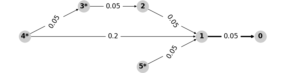
Figure 4 is an example attack graph, which will be used as a running example for TDCycle.


We then convert the resulting tree decomposition into a nice tree decomposition Cygan et al. 2015, as illustrated in Figure 6. The root node is a bag containing DA only and all the leaf nodes are bags of size one.77 7 The standard nice tree decomposition definition involves empty bags. For example, a leaf node in our illustration contains one vertex, which can be interpreted as an introduce node by adding an auxiliary empty bag as its child. We ignore empty bags as they play no role in our DP. In a nice tree decomposition, there are only three types of nodes.
- •
Introduce node: An introduce node has an only child . and has size . For example, in Figure 6, is an introduce node.
- •
Forget node: A forget node has an only child . and has size . For example, in Figure 6, is a forget node.
- •
Join node: A join node has two children. must be identical to both children. For example, in Figure 6, is a join node.
It is a trivial task to convert a tree decomposition into a nice tree decomposition. For example, in Figure 5, splits into two branches. We just need to add two clones of it to make it a valid join node. As another example, in Figure 5, is connected to directly. By inserting in between, (top-left one among the three clones) becomes an introduce node and becomes a forget node. A tree decomposition with tree width can be converted to a nice tree decomposition with nodes.
The whole point of nice tree decomposition is to divide the nodes into three categories, so that when we design DP, we just need to come up with three rules (one rule for each category of nodes).

7.5 TDCycle example based on Figure 6
Proof of Lemma 1.
Let be an edge in the attack graph. In any tree decomposition, there must be a bag that contains both and . We check the parent of . If the parent also contains both and , then we keep going up, until one of or is forgotten. (Both cannot be forgotten at the same node, since exactly one is forgotten at a forget node under a nice tree decomposition.) The forget node where either or is forgotten is the node we assign to. The above forget node is unique for the following reasons. A known property of tree decomposition is that a node is forgotten at a unique forget node. The forget node for and must satisfy that either the forget node for is an ancestor of the forget node for (in which case is assigned to the forget node for ), or the reverse. This is because the subgraphs induced by or must be trees. That is, at the above unique forget node, we decide whether or not to block . ∎
Recall that in our DP, for every node , there is a corresponding subproblem , which returns the collection of all possible tuples (distance matrix achieved and budget spent) after processing , where is the subtree rooted at . In our example, all edges have the same failure rate , which translates to a distance of .
- •
Base cases: There are only two leaf nodes and . At leaf nodes, we have not put back any edges at all. is not an entry vertex, so after processing , the only possible tuple is . That is,
Similarly, since is an entry vertex, we have
- •
Original problem: We have set a budget of . The root node is . After processing all nodes, we have
That is, after processing all nodes in the nice tree decomposition, we end up with two possible tuples. We can spend units of budget to ensure that the attacker’s distance to (DA) is , which translates to a success rate of . We can also spend units of budget to ensure that the attacker’s distance to (DA) is , which translates to a success rate of . Given a budget of , we conclude that the attacker’s worst success rate is .
In our implementation, we have a micro-optimisation step that filtered out as this tuple is worse off than . Given two different tuples and , if and (every element of is larger or equal), then is discarded.
- •
Introduce node: is an introduce node. is introduced at this node, but its edges have not been put back yet, so is disconnected. is also not an entry vertex. Since , we have
is another introduce node. is introduced at this node. Its edges have not been put back yet, but is an entry vertex. So we have
The in the above matrix (top-left corner) indicates that the distance from to an entry vertex is (as is an entry vertex itself).
- •
Forget node: is a forget node. is forgotten here. That is, we need to consider putting back some edges. The two edges assigned to this forget node is and . We must put back as it is not blockable. For , we either block it or not. If we do not block , then we end up with the following possible tuple:
The interpretation is that after putting back both and , the end result is as follows:
- –
top left : it takes hops to go from an entry vertex to
- –
top right : it takes hops to go from to
- –
bottom left : we cannot go from to (note: the edge has not been put back yet)
- –
bottom right : it takes hops to go from an entry vertex to
If we block , then we end up with the following possible tuple:
In summary, we have
- –
- •
Join node: In Figure 6, there are three clones of . We use , and to denote the one on the right, top and bottom, respectively.
We directly present the values of and .
is
is
is then the aggregation of the above. We take one tuple from and one tuple from . We add into , provided that . is
7.6 Pseudocode of TDCycle
We present the pseudocode of TDCycle in this section.
TDCycle base cases setup
Input: Nice tree decomposition TD
TDCycle final step after finishing DP Input:
TDCycle at introduce node
Input: Nice tree decomposition TD
Introduce node
’s child
TDCycle at forget node
Input: Nice tree decomposition TD
Forget node
’s child
TDCycle at join node
Input: Nice tree decomposition TD
Join node
Two children and
7.7 Complexity of TDCycle
Proof of Theorem 2.
There are DP subproblems in total, which fall into three categories as follows. The return value of is a collection. We use a binary array to represent this collection. The size of the array is , or simply .88 8 In experiments, we used Python’s builtin set instead, because most tuples are not possible.
- •
Introduce node: We need to go through the child node’s output array (at most tuples) and expand the distance matrix by one row and one column. The complexity is for each tuple. There are at most introduce nodes. So the complexity for handling all introduce nodes is .
- •
Forget node: We need to go through the child node’s output array (at most tuples) and shrink the distance matrix by one row and one column. The complexity is for each tuple as we need to run an all pair shortest path for each blocking option and there are options. There are at most forget nodes (a vertex is forgotten once). So the complexity for handling all forget nodes is .
- •
Join node: We need to go through both children nodes’ output arrays (at most pairs of tuples). We need to perform an element-wise min operation on the distance matrices, which has a complexity of . There are at most join nodes. So the complexity for handling all join nodes is .
We do not need to run an all-pair shortest path update at a join node. If the join node has a bag size of , then all-pair shortest path is not necessary. If the bag size is more than , then there will be forget nodes between the join node and root. We could wait until we reach a forget node to run the all-pair shortest path process.
Assuming is at least , the overall complexity is then
∎
It should be noted that the above is the worst case complexity. In experiments, the set size of is often quite small (i.e., in the hundreds for R2000).
7.8 , when restricted to a small interval, can be approximated using two straight lines (one upper bound and one lower bound)

7.9 Reproducibility notes and preprocessing steps
We have included our source code as well as the synthetic AD graphs. R2000 and R4000 were generated using DBCreator by setting the numbers of computers to and , respectively. ADS10 was generated using adsimulator with the following parameters: nComputers=1000, nUsers=1000, nOUs=200, nGroups=1000, nGPOs=200.
Both tools are open source and are available at:
https://github.com/BloodHoundAD/BloodHound-Tools/tree/master/DBCreator
https://github.com/nicolas-carolo/adsimulator
In our experiments, we run trials with different random setups (randomly picked blockable edges and entry nodes). The trials are using fixed random seeds from to . For MIP-Feasible and MIP-LB, we used regions to approximate : .
Before running our algorithms, we perform the following preprocessing steps:
- •
In both R2000 and R4000, there are admin nodes. In ADS10, there are admin nodes (nodes whose admincount property is true). We merge them into a single destination node and set it as DA. We ignore all out-going edges of DA. (Once the attacker reaches DA, the attack has finished.)
- •
We delete all nodes that cannot reach DA.
- •
We delete all incoming edges to entry nodes, because the optimal attack path will never involve such edges.
- •
We delete non-entry nodes that have in-degrees, because the attacker cannot start from these nodes or reach these nodes.
- •
If an edge is not block-worthy (Lemma 2), then we mark it as not blockable.
- •
For a splitting node , if there are two non-splitting paths and that satisfy: 1) these two paths have the same end node (); 2) the first path has a higher success rate (); 3) The first path is not blockable, then the attacker always prefers the first path (facing any defense). We delete as it is never used.
7.10 Proximal Policy Optimization parameters and implementation details
We used the PPO implementation from the popular Tianshou library, with the following parameters. Our code is also included.
| learning rate | |
|---|---|
| discount factor | |
| batch size | |
| epoch | refer to experiment description |
| step per epoch | |
| step per collect | |
| repeat per collect | |
| hidden sizes | for R2000 |
| for others |
The observation space is a tuple where every coordinate is between and . An observation consists of the following:
- •
Distance matrix before blocking: The length is the square of the maximum tree decomposition bag size. Every matrix element is expressed in terms of probability so it is between and . If the current bag size is less than the maximum bag size, then we only use the “top left” corner. The remaining slots are filled in with s (equivalent to adding auxiliary nodes that not connected to any other nodes).
- •
Distance matrix after blocking.
- •
Budget spent: if the total budget is and is left, then we append to the observation.
- •
Current step index: if the total episode length is and we have finished steps, then we append to the observation.
7.11 Experiments showing that our RL based approach is not merely performing random searching and the tree decomposition based distance matrix indeed provides a useful representation that facilitates learning
We conduct experiments by running reinforcement learning on the original observation space with the tree decomposition based distance matrix. We then repeat the experiments using the same setups and the same random seeds, but we replace the actual distance matrix by the zero matrix and by the random matrix. For a fair comparison, we do not modify the representation for the budget spent and the current step index. Our experiments show that learning significantly deteriorates after the replacements.
We design the following AD graph for our experiments. Node is DA. Besides DA, we have entry nodes from node to node . Node () has one blockable edge pointing to DA. These are all the edges in the graph. We set a budget of . That is, we need to block half of the edges. For that is even, the failure rate of edge is , which represents an edge that does not need to be blocked as the failure rate is high. For that is odd, the failure rate of edge is (), which represents an edge that needs to be blocked considering that our budget is . The design motivation of this AD graph is as follows:
- •
The task is to pick out “correct” edges to block out of edges, which has a large search space (over ).
- •
The attacker’s best success rate is , which happens as long as is not blocked. That is, with this one mistake, we end up with the worst performance. The attacker’s worst success rate is , which only happens when every edge blocked is “correct”. There is a wide range of possible results between and and it gets increasingly difficult to achieve better performance.
- •
We intertwine the block-worthy and not-block-worthy edges so that we do not accidentally learn toward policies such as “spend all budget immediately” (if all block-worthy edges have lower indices) or “spend all budget at the end” (if all not-block-worthy edges have lower indices). It should be noted that the edges’ indices are not included in the observation, so we will not accidentally learn toward “block odd edges”.
We use Original to represent the original approach with the distance matrix intact. We use Zero and Random to represent the results after replacing the distance matrix using the zero matrix and the random matrix (every matrix element independently drawn from ). We record the worst success rate for the attacker after and epochs. Experiments are repeated times using training seed from to . The table cells are the averages and the standard deviations over these trials. Clearly, the tree decomposition based distance matrix provides a useful representation that facilitates learning (smaller numbers are better).
| Epochs | Original | Zero | Random |
|---|---|---|---|
Lastly, we run experiments on R2000 with budget . We use the same experimental setup as before (as described in the experiment section). We randomly draw the entry nodes and the blockable edges using random seed to . Experiments are repeated times using training seed from to . We record the worst success rate for the attacker after and epochs (due to time constraint – as we are running three experiments for random graphs and for training seeds, which in total equals experiments). For seed , every trial reaches optimality within epochs, so we only present the result for seed . The numbers do not differ much because 1) the gap between the optimal result and the greedy result is tiny to begin with; 2) the search space isn’t large (given enough time, random searching often can find the optimal result for this graph). Still, we see that the original approach always produces the best result.
| R2000 | Original | Zero | Random |
| epochs | |||
| Seed | |||
| Seed | |||
| Seed | |||
| Seed |
| R2000 | Original | Zero | Random |
| epochs | |||
| Seed | |||
| Seed | |||
| Seed | |||
| Seed |
7.12 Description of the kernel
Due to space constraint, we did not explicitly mention what the kernel is in our section on kernelization. Also, for presentation purpose, we want to avoid confusion by brining up a different graph. For completeness, the kernel is as follows: Only keep splitting nodes, entry nodes and DA. Delete all original edges. Replace every original non-splitting path by one edge. The edge’s success rate is the unblocked success rate of the original non-splitting path. The edge is blockable if and only if the original non-splitting is blockable.
7.13 More on TDCycle vs IP
As shown in our experiments, IP scales extremely well and performs much better than TDCycle on all three graphs generated using two different open source AD graph generators. We expect TDCycle to perform relatively better if we are dealing with a graph with a small tree width and a large number of non-splitting paths. As an example, let us consider the following contrived attack graph. There is one entry node called entry and one DA. We insert the following edges: entry DA for from to (that is, there are in total nodes). All edges are set to be blockable and have the same failure rates. This attack graph has a tree width of . The maximum attack path length is . The number of possible success rates for attack paths is . With the above set up, TDCycle’s complexity becomes . On the contrary, for IP, we face an integer program with binary variables.
Lastly, TDCycle has two advantages over IP:
- •
TDCycle is embarrassingly parallel. That is, if we throw CPU cores to it, we expect about times speed up. For all three types of nodes (introduce/forget/join), the main calculation is a for loop that can be trivially made parallel. Given a node , we just need to use a shared memory array to store the result for . All parallel processes can write to this shared array without worrying about race condition.
On the contrary, IP is difficult to be made parallel.
- •
TDCycle does not require that we load the whole model into the memory. Memory paging is convenient under TDCycle. The dynamic program is in a bottom-up fashion. Node in the tree decomposition requires a memory block to store its result . For node , we only need to allocate memory for it once we reach it. Also, after processing a node, we can safely delete the memory blocks for the children nodes.
On the contrary, memory paging is difficult for IP.