Bi-Yang–Baxter Models and Sl(2)-orbits

The bi-Yang–Baxter model lies in the class of Yang–Baxter deformations of non-linear $\sigma$-models, all of which involve an object called the (classical) $R$-matrix. It is an endomorphism of the Lie algebra $\mathfrak{g}$, i.e. a linear map

$$R:\mathfrak{g}\rightarrow\mathfrak{g}\,,$$

(2.3)

satisfying the modified classical Yang–Baxter equation

$$[RX,RY]-R\left([RX,Y]+[X,RY]\right)=-c^{2}[X,Y]\,,\qquad\forall X,Y\in\mathfrak{g}\,,$$

(2.4)

where $c^{2}$ is a real constant. The word ‘modified’ refers to the fact that $c$ is allowed to be non-zero. Note that by a real rescaling of $R$ we may restrict to the cases $c\in\{0,1,i\}$. In the following, we will additionally impose the condition that $R$ is skew-symmetric with respect to the chosen bilinear form on $\mathfrak{g}$. In other words

$$(RX,Y)+(X,RY)=0\,,\qquad\forall X,Y\in\mathfrak{g}\,.$$

(2.5)

Such $R$-matrices are also referred to as Yang–Baxter operators and have been classified in the mathematics literature [7], see also [21].

There is a standard solution to the modified classical Yang–Baxter equation, given by the Drinfel’d–Jimbo solution [5, 6]. In order to write it down, let us first consider the complexification $\mathfrak{g}_{\mathbb{C}}$ of $\mathfrak{g}$ and let $\mathfrak{h}$ be a Cartan subalgebra of $\mathfrak{g}_{\mathbb{C}}$. Then $\mathfrak{g}_{\mathbb{C}}$ enjoys a root space decomposition

$$\mathfrak{g}_{\mathbb{C}}=\mathfrak{h}\oplus\bigoplus_{\alpha}\mathfrak{g}_{\alpha}\,,$$

(2.6)

where $\alpha\in\mathfrak{h}^{*}$ runs over all the roots and each $\mathfrak{g}_{\alpha}$ denotes the root space associated to a root $\alpha$. A choice of simple roots fixes a notion of positive roots, denoted by $\alpha>0$. Let $\{H^{\mu},E^{\pm\alpha}\}$ denote a Cartan–Weyl basis of $\mathfrak{g}_{\mathbb{C}}$, where $\alpha$ runs over the positive roots. These generators satisfy the usual commutation relations

$$[H^{\mu},H^{\nu}]=0\,,\qquad[H^{\mu},E^{\pm\alpha}]=\pm\alpha(H^{\mu})E^{\pm\alpha}\,.$$

(2.7)

In terms of this basis, the Drinfel’d–Jimbo $R$-matrix is defined as²² 2 The overall sign of $R$ is, of course, a matter of convention. Here we have chosen the sign to match with [1].

$$RH^{\mu}=0\,,\qquad RE^{\pm\alpha}=\mp c\,E^{\pm\alpha}\,.$$

(2.8)

One can verify by direct computation that (2.8) solves the modified classical Yang–Baxter equation (2.4) and that it satisfies the skew-symmetry condition (2.5). However, it is important to keep in mind that the above $R$-matrix is defined on the complexified algebra $\mathfrak{g}_{\mathbb{C}}$. Depending on the choice of real form $\mathfrak{g}$ and the constant $c$, it may happen that $R$ is not a real endomorphism of $\mathfrak{g}$. For further details we refer the reader to the lecture notes of B. Hoare [1].

For a given choice of Yang–Baxter operator $R$, the action of the associated bi-Yang–Baxter model is given by

$$S=\int_{\Sigma}d^{2}\sigma\,\left(g^{-1}\partial_{+}g\,,\frac{1}{1-\eta R-\zeta R^{g}}g^{-1}\partial_{-}g\right)\,,$$

(2.9)

where $\eta$ and $\zeta$ are two constants parametrizing the deformation, and we have introduced the notation

$$R^{g}:=\mathrm{Ad}_{g^{-1}}\circ R\circ\mathrm{Ad}_{g}\,.$$

(2.10)

Clearly, for $\eta=\zeta=0$ one recovers the action of the principal chiral model, which enjoys a global $G_{L}\times G_{R}$ symmetry. Keeping $\zeta=0$ but letting $\eta$ be non-zero, the introduction of the operator $R$ breaks the global $G_{R}$ symmetry down to the $\mathrm{U}(1)_{R}^{\mathrm{rk}\,G}$ subgroup. In this case, one retrieves the action of the (single-parameter) Yang–Baxter model, which is also referred to as the $\eta$-model [22]. Upon letting $\zeta$ be non-zero also the global $G_{L}$ symmetry is broken down to the $\mathrm{U}(1)_{L}^{\mathrm{rk}\,G}$ subgroup.

There is a special point in the parameter space where the symmetry of the bi-Yang–Baxter model is enhanced [9]. Indeed, whenever $\zeta=\eta$, which we will refer to as the critical line following [8], one has an additional symmetry given by $g\mapsto g^{-1}$. The critical bi-Yang–Baxter model will play a crucial role in this work, as we will find a set of solutions to the model which solve the model precisely when $\zeta=\eta$. There have been a number of observations that indicate that the critical bi-Yang–Baxter model can be related to other integrable models. For example, the critical $\mathrm{SU}(2)$ bi-Yang–Baxter model is equivalent to the coset $\mathrm{SO}(4)/\mathrm{SO}(3)$ $\eta$-model [10, 11]. Furthermore, at the conformal point $\zeta=\eta=\frac{i}{2}$ the target space geometry coincides with that of the $\mathrm{SU}(1,1)/\mathrm{U(1)}$ gauged WZW model with an additional $\mathrm{U}(1)$ boson [11].

In order to write down the equations of motion of the bi-Yang–Baxter model, it is convenient to introduce the currents (we follow the conventions of [9])

$$J_{\pm}=\mp\frac{1}{1\pm\eta R\pm\zeta R^{g}}j_{\pm}\,,\qquad j_{\mu}=g^{-1}\partial_{\mu}g\,.$$

(2.11)

In terms of $J_{\pm}$, the equations of motion read

$$\partial_{+}J_{-}-\partial_{-}J_{+}-\eta[J_{+},J_{-}]_{R}=0\,,$$

(2.12)

where

$$[X,Y]_{R}:=[RX,Y]+[X,RY]\,,\qquad\forall X,Y\in\mathfrak{g}\,,$$

(2.13)

defines a second Lie-bracket on $\mathfrak{g}$, by virtue of the classical Yang–Baxter equation (2.4). It is referred to as the $R$-bracket and is central for the underlying Poisson-Lie symmetry of the bi-Yang–Baxter model, see e.g. [23].

It was shown by C. Klimčík in [9] that the bi-Yang–Baxter model is classically integrable. Vital in this regard is the condition that $R$ satisfies the modified classical Yang–Baxter (2.4) equation and is anti-symmetric. The integrability condition means that the equations of motion of the bi-Yang–Baxter model can be reformulated as the zero-curvature condition of a Lax connection

$$\mathcal{L}_{\pm}(\lambda)=\left(\eta(R-i)+\frac{2i\eta\pm(1-\eta^{2}+\zeta^{2})}{1\pm\lambda}\right)J_{\pm}\,,$$

(2.14)

where $\lambda\in\mathbb{C}$ is the spectral parameter. More precisely, introducing the connection

$$\nabla_{\pm}=\partial_{\pm}+\mathcal{L}_{\pm}(\lambda)\,,$$

(2.15)

the zero-curvature condition simply states that

$$[\nabla_{+},\nabla_{-}]=0\,,$$

(2.16)

for all $\lambda$. This is equivalent to the equations of motion (2.12) together with the Bianchi identities for $J_{\pm}$. The flatness of the Lax connection ensures the existence of an infinite tower of conserved charges. The Hamiltonian integrability of the model, i.e. the condition that all these charges in fact Poisson-commute with each other, was established in [24].

For $\mathfrak{su}(2)$, the solution to the modified Yang–Baxter equation is essentially unique and is given by the Drinfel’d–Jimbo solution discussed in the previous section. Let us go through the construction of the $R$-matrix in some detail. The complexification of $\mathfrak{su}(2)$ is $\mathfrak{sl}(2,\mathbb{C})$, which has a Cartan–Weyl basis given by

$$H=\begin{pmatrix}1&0\\ 0&-1\end{pmatrix}\,,\qquad E_{+}=\begin{pmatrix}0&1\\ 0&0\end{pmatrix}\,,\qquad E_{-}=\begin{pmatrix}0&0\\ 1&0\end{pmatrix}\,,$$

(2.17)

satisfying

$$[H,E_{\pm}]=\pm 2E_{\pm}\,.$$

(2.18)

Using (2.8) we obtain a solution to the modified classical Yang–Baxter equation, at the level of $\mathfrak{sl}(2,\mathbb{C})$. In order to see if this descends to a real solution when restricting to the real form $\mathfrak{su}(2)$, let us fix a basis of $\mathfrak{su}(2)$ as $T_{j}=i\sigma_{j}$, where $\sigma_{i}$ denote the Pauli matrices. Then one readily finds that $R$ acts on this basis as

$$RT_{1}=-ic\,T_{2}\,,\qquad RT_{2}=ic\,T_{1}\,,\qquad RT_{3}=0\,.$$

(2.19)

In particular, for $R$ to be a real endomorphism we require $c=i$, in which case $R$ can be represented as a matrix in the $T_{i}$ basis as

$$R=\begin{pmatrix}0&-1&0\\ 1&0&0\\ 0&0&0\end{pmatrix}\,.$$

(2.20)

In the remainder of this section, we will implicitly use this $R$-matrix.

We will adopt the following parametrization of the $\mathrm{SU}(2)$ group element

$$g=\begin{pmatrix}\cos\theta\,e^{i\phi_{1}}&i\sin\theta\,e^{i\phi_{2}}\\ i\sin\theta\,e^{-i\phi_{2}}&\cos\theta\,e^{-i\phi_{1}}\end{pmatrix}\,,\qquad\theta,\phi_{1}\in[0,\pi)\,,\quad\phi_{2}\in[0,2\pi)\,.$$

(2.21)

As a non-linear $\sigma$-model, the bi-Yang–Baxter model can be characterized by the metric and $B$-field it induces on the target space. These follow from inserting the ansatz (2.21) for $g$, together with the $R$-matrix (2.20), into the action (2.9). The resulting metric reads

	$\displaystyle ds^{2}$	$\displaystyle=\frac{1}{\Delta}\left[\mathrm{d}\theta^{2}+\cos^{2}\theta\left(1+(\eta+\zeta)^{2}\cos^{2}\theta\right)\mathrm{d}\phi_{1}^{2}+\sin^{2}\theta\left(1+(\eta-\zeta)^{2}\sin^{2}\theta\right)\mathrm{d}\phi_{2}^{2}\right]$
		$\displaystyle\qquad+\frac{\sin^{2}(2\theta)}{2\Delta}(\eta-\zeta)(\eta+\zeta)\mathrm{d}\phi_{1}\mathrm{d}\phi_{2}\,,$

where we have defined

$$\Delta=1+\eta^{2}+\zeta^{2}+2\eta\zeta\cos(2\theta)\,.$$

(2.22)

Moving on, the $B$-field is found to be pure-gauge, and given is by

$$B=\mathrm{d}A\,,\qquad A=\frac{\log\Delta}{4\eta\zeta}\left[(\eta-\zeta)\mathrm{d}\phi_{1}-(\eta+\zeta)\mathrm{d}\phi_{2}\right]\,.$$

(2.23)

The form of the metric and $B$-field indicate that at the points $\zeta=\eta$ and $\zeta=-\eta$ the model simplifies significantly. We recall that the point $\zeta=\eta$ is referred to as the critical line. In contrast, the point $\zeta=-\eta$ is referred to as the co-critical line. As alluded to before, on the critical line this simplification is due to the emergence of the $\mathbb{Z}_{2}$ symmetry $g\mapsto g^{-1}$. In the parametrization (2.21) this corresponds to

$$\phi_{1}\mapsto-\phi_{1}\,,\qquad\phi_{2}\mapsto\phi_{2}+\pi\,.$$

(2.24)

However, note that for the $\mathrm{SU}(2)$ model in particular there is an additional $\mathbb{Z}_{2}$-symmetry given by the transformations

$$\theta\mapsto\theta+\frac{\pi}{2}\,,\qquad\phi_{1}\leftrightarrow\phi_{2}\,,\qquad\zeta\mapsto-\zeta\,.$$

(2.25)

This exactly maps the critical line $\zeta=\eta$ to the co-critical line $\zeta=-\eta$.

The unitons are finite action solutions to the classical equations of motion of the $\mathrm{SU}(2)$ bi-Yang–Baxter model, which additionally satisfy $g^{2}=-1$. In the parametrization (2.21), this condition imposes that either $\theta=\frac{\pi}{2}$ or $\phi_{1}=\frac{\pi}{2}$. We will consider the latter case. There are two types of unitons, dubbed the real and complex unitons. Both are determined by the choice of a holomorphic function $f(z)$ of the worldsheet coordinate. The expressions for $\phi_{1}$ and $\phi_{2}$ are the same for both unitons, and are given by

$$\phi_{1}=\frac{\pi}{2}\,,\quad\phi_{2}=\pi+\frac{i}{2}\log\left(\frac{f}{\bar{f}}\right)\,,$$

(2.26)

while the expressions for $\theta$ differ and are respectively given by

	$\displaystyle\text{real uniton}:\qquad\sin^{2}\theta$	$\displaystyle=\frac{4|f|^{2}}{(1+|f|^{2})^{2}+(\eta-\zeta)^{2}(1-|f|^{2})^{2}}\,,$		(2.27)
	$\displaystyle\text{complex uniton}:\qquad\theta$	$\displaystyle=\frac{\pi}{2}+i\arctanh\left(\frac{1}{2}\left(|f|+\frac{1}{|f|}\right)\sqrt{(\eta-\zeta)^{2}+1}\right)\,.$		(2.28)

The nomenclature ‘real’ vs. ‘complex’ is due to the fact that for the real uniton, $\theta$ is manifestly real and hence the group-valued field $g$ indeed lies in $\mathrm{SU}(2)$. In contrast, for the complex uniton $\theta$ is complex-valued and hence $g$ takes values in the complexified group $\mathrm{SL}(2,\mathbb{C})$.³³ 3 Note that for real $x$ $$\mathrm{Im}\,\arctanh\,x=\begin{cases}0\,,&|x|<1\,,\\ -\frac{\pi}{2}\mathrm{sign}(x)\,,&|x|>1\,.\end{cases}$$ Therefore, one finds that for the complex uniton $\mathrm{Re}\,\theta=\pi$, hence $g$ in fact takes values in $\mathrm{SU}(1,1)$. See also the discussion in section 2.3.

For completeness, we also record the metric of the $\mathrm{SU}(2)$ bi-Yang–Baxter model when evaluated on the real and complex unitons. Introducing polar coordinates $f=re^{i\alpha}$ and writing $R=r^{2}$ one finds⁴⁴ 4 Here we have used the fact that $$4R^{2}\left(\frac{\mathrm{d}\theta}{\mathrm{d}R}\right)^{2}=\sin^{2}\theta+(\zeta-\eta)^{2}\sin^{4}\theta\,,$$ which holds for both the real and complex uniton and can be verified by explicit computation.

$$ds^{2}=\frac{1}{\Delta}\left(\frac{\mathrm{d}\theta}{\mathrm{d}R}\right)^{2}\left(\mathrm{d}R^{2}+4R^{2}\mathrm{d}\alpha^{2}\right)\,,$$

(2.29)

for both unitons. We see that in the target space the uniton solutions correspond to a squashed two-sphere inside $\mathrm{SU}(2)$. From here it follows from explicit integration that the unitons have finite action and we refer the reader to [8] for further details. One finds that the on-shell actions evaluate to (we neglect the overall factor coming from the angular integration)

$$S_{\text{real uniton}}=\frac{1}{2\eta\zeta}\left[(\eta+\zeta)\arctan(\eta+\zeta)-(\eta-\zeta)\arctan(\eta-\zeta)\right]\,,$$

(2.30)

and

$$S_{\text{complex uniton}}=\frac{1}{2\eta\zeta}\left[(\eta+\zeta)\arccot(\eta+\zeta)-(\eta-\zeta)\arccot(\eta-\zeta)\right]\,.$$

(2.31)

Here we have assumed the domain of integration to be the entire complex plane. In other words, $R$ ranges from 0 to infinity. In the next section we will encounter a situation where $f(z)$ instead takes values in the unit disk, in which case $R\in[0,1]$. One can verify that this only changes the above results by a factor of 1/2.

Let us start by introducing the Weil operator of the torus. A convenient description of the torus $\mathbb{T}$ is as a lattice

$$\mathbb{T}=\mathbb{C}/(\mathbb{Z}+\tau\mathbb{Z})\,,\qquad\mathrm{Im}\,\tau>0\,,$$

(2.32)

where $\tau$ is the Teichmüller parameter taking values in the complex (strict) upper half-plane. We parametrize the torus by two periodic coordinates $\xi_{1},\xi_{2}$ with $\xi_{i}\sim\xi_{i}+1$. Then the metric on the torus can be written as

$$ds^{2}=\frac{|\mathrm{d}\xi_{1}+\tau\,\mathrm{d}\xi_{2}|^{2}}{\mathrm{Im}\,\tau}\,.$$

(2.33)

Here we have normalized the metric so that the torus has unit volume. The Weil operator is closely related to the Hodge star operator on the torus. The action of the Hodge star on the one-forms $\mathrm{d}\xi_{1}$ and $\mathrm{d}\xi_{2}$ follows directly from the metric (2.33) and is given by

$$\star\,\mathrm{d}\xi_{1}=\frac{\mathrm{Re}\,\tau}{\mathrm{Im}\,\tau}\mathrm{d}\xi_{1}+\frac{|\tau|^{2}}{\mathrm{Im}\,\tau}\mathrm{d}\xi_{2}\,,\qquad\star\,\mathrm{d}\xi_{2}=-\frac{1}{\mathrm{Im}\,\tau}\mathrm{d}\xi_{1}-\frac{\mathrm{Re}\,\tau}{\mathrm{Im}\,\tau}\mathrm{d}\xi_{2}\,.$$

(2.34)

To obtain the Weil operator, one should view this as an action on the middle de Rham cohomology of the torus. Indeed, in the basis $\{[\mathrm{d}\xi_{1}],[\mathrm{d}\xi_{2}]\}$, where $[\omega]$ denotes the equivalence class of a one-form $\omega$, the action of the Hodge star can be represented as a matrix

$$C(x,y)=\frac{1}{y}\begin{pmatrix}x&-1\\ x^{2}+y^{2}&-x\end{pmatrix}\,,$$

(2.35)

where we have set $\tau=x+iy$. We will refer to (2.35) as the Weil operator of the torus. Note that it is an element of $\mathrm{SL}(2,\mathbb{R})$.

An interesting property of (2.35) is that it satisfies⁵⁵ 5 More generally, the origin of this relation is the fact that $\star\star$ evaluates to $\pm 1$, with the sign determined by the degree of the differential form it acts on and the dimension of the spacetime in question.

$$C^{2}=-1\,,$$

(2.36)

which is shared by the unitons solutions discussed in section 2. In fact, we will now argue that the Weil operator can be viewed as a complex uniton for a specific choice of the holomorphic function $f(z)$.

As a preliminary remark, we stress that one cannot simply compare the expressions (2.21) and (2.35), as the two lie in different groups, namely $\mathrm{SU}(2)$ and $\mathrm{SL}(2,\mathbb{R})$, respectively. There is, however, a natural two-step procedure to pass between the two groups by combining a so-called Cayley transformation with an analytic continuation. Let us first elaborate on the former. We introduce the matrix

$$\rho=\frac{1}{\sqrt{2}}\begin{pmatrix}1&i\\ i&1\end{pmatrix}\,,$$

(2.37)

which is an element of $\mathrm{SL}(2,\mathbb{C})$. Then it is straightforward to show that the adjoint action

$$\mathrm{Ad}_{\rho}:\mathrm{SL}(2,\mathbb{R})\rightarrow\mathrm{SU}(1,1)$$

(2.38)

is an isomorphism of real Lie groups, which is commonly referred to as a Cayley transformation. Indeed, it provides an interpolation between the two real forms $\mathrm{SL}(2,\mathbb{R})$ and $\mathrm{SU}(1,1)$ of $\mathrm{SL}(2,\mathbb{C})$. For the second step of the proposed procedure, one interpolates between $\mathrm{SU}(1,1)$ and $\mathrm{SU}(2)$ via an analytic continuation. In the parametrization (2.21) this is straightforwardly given by sending $\theta\mapsto-i\theta$.

We now apply the above procedure to compare the Weil operator of the torus to a generic element in $\mathrm{SU}(2)$. Practically, it is easiest to take the expression in (2.21), analytically continue it to $\mathrm{SU}(1,1)$ by setting $\theta=i\tilde{\theta}$ and then apply $\mathrm{Ad}_{\rho^{-1}}$ to end up in $\mathrm{SL}(2,\mathbb{R})$. The result of this computation is

$$g_{\mathrm{SL}(2,\mathbb{R})}=\begin{pmatrix}\cosh\tilde{\theta}\cos\phi_{1}-\sinh\tilde{\theta}\sin\phi_{2}&-\cosh\tilde{\theta}\sin\phi_{1}-\sinh\tilde{\theta}\cos\phi_{2}\\ \cosh\tilde{\theta}\sin\phi_{1}-\sinh\tilde{\theta}\cos\phi_{2}&\cosh\tilde{\theta}\cos\phi_{1}+\sinh\tilde{\theta}\sin\phi_{2}\end{pmatrix}\,,$$

(2.39)

which is indeed an element of $\mathrm{SL}(2,\mathbb{R})$. Comparing (2.35) and (2.39) and solving for $\tilde{\theta},\phi_{1},\phi_{2}$ in terms of $x,y$ gives

$$\phi_{1}=\frac{\pi}{2}\,,\qquad\phi_{2}=\pi+\frac{i}{2}\log\left(\frac{f}{\bar{f}}\right)\,,\qquad\tilde{\theta}=\frac{i\pi}{2}+\arctanh\left[\frac{1}{2}\left(|f|+\frac{1}{|f|}\right)\right]\,,$$

(2.40)

where $f(z)$ is the following holomorphic function of the complexified worldsheet coordinates

$$f(z)=\frac{z-i}{z+i}\,,\qquad z=x+iy\,.$$

(2.41)

Indeed, identifying the Teichmüller parameter $\tau$ with the worldsheet coordinate $z$ and recalling that $\theta=i\tilde{\theta}$, one sees that this solution is precisely of the form of a complex uniton (2.28) with additionally $\zeta=\eta$.⁶⁶ 6 Strictly speaking, an exact match is obtained after sending $\theta\mapsto\theta+\pi$, corresponding to $C\mapsto-C$. Of course, the overall sign of $C$ is simply a convention. The function $f(z)$ is a special type of Möbius transformation that conformally maps the upper half-plane to the unit disc. Note that it is holomorphic on the upper half-plane, but has a first order pole at $z=-i$.

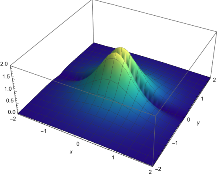
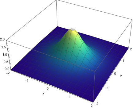
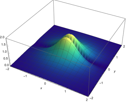
In figure 1 we have illustrated the Lagrangian density for the complex uniton defined by the particular holomorphic function (2.41). It is interesting to contrast this with the plots in [8], where instead a linear function $f(z)=\frac{z}{2}$ was used. In both cases there is a clear transition at the critical point $\zeta=\eta$. On the other hand, the concentric valley structure in [8] is not present here. Rather, in our case the density is not rotationally invariant, but only invariant under reflections $x\mapsto-x$ and $y\mapsto-y$. Of course, this can be explained by noting that the Lagrangian density is a function of $|f(z)|$.

It is also interesting to recall the $\mathbb{Z}_{2}$-symmetry (2.25) which maps the critical line to the co-critical line. Indeed, one finds that it acts on the Weil operator as

$$C(x,y)\mapsto\frac{i}{y}\begin{pmatrix}-1&-x\\ x&x^{2}+y^{2}\end{pmatrix}=C(x,y)\cdot\begin{pmatrix}0&i\\ i&0\end{pmatrix}\,.$$

(2.42)

Interestingly, the $\mathbb{Z}_{2}$ transformation can be described as a right-multiplication of $C(x,y)$ by an element in $\mathrm{SL}(2,\mathbb{C})$ (even in $\mathrm{SU}(2)$). However, as a result the transformed Weil operator is no longer real-valued. Therefore, it will define a solution to the co-critical $\mathrm{SL}(2,\mathbb{C})$ bi-Yang–Baxter model, as can be verified by explicit computation.

As a final comment, one can use the result (2.29), taking $f(z)$ as above, to find that the on-shell metric is given by

$$ds^{2}=\frac{4|\mathrm{d}z|^{2}}{(z-\bar{z})^{2}-4\eta^{2}(1+|z|^{2})^{2}}\,.$$

(2.43)

Note that in the limit $\eta\rightarrow 0$ one recovers the standard metric on the Poincaré upper half-plane.

As a result of the identification between the Weil operator and a complex uniton, one expects that the Weil operator provides a solution to the $\mathrm{SL}(2,\mathbb{R})$ bi-Yang–Baxter model. To make this precise, one should also identify the appropriate $R$-matrix by taking the $\mathrm{SU}(2)$ $R$-matrix in (2.20) and translating it to an endomorphism of $\mathrm{SL}(2,\mathbb{R})$ via the Cayley transform. Explicitly, this gives⁷⁷ 7 One can check that the $R$-matrix remains unchanged under the analytic continuation from $\mathrm{SU}(2)$ to $\mathrm{SU}(1,1)$.

$$R_{\mathrm{SL}(2,\mathbb{R})}=\mathrm{Ad}_{\rho^{-1}}\circ R_{\mathrm{SU}(2)}\circ\mathrm{Ad}_{\rho}\,.$$

(2.44)

One can verify that the resulting $R$-matrix acts as

$$R_{\mathrm{SL}(2,\mathbb{R})}\,H=-(E_{+}+E_{-})\,,\qquad R_{\mathrm{SL}(2,\mathbb{R})}\,E_{\pm}=\frac{1}{2}H\,,$$

(2.45)

and is manifestly real. The reader is invited to check that indeed the Weil operator (2.40) is a solution to the critical $\mathrm{SL}(2,\mathbb{R})$ bi-Yang–Baxter model defined by the $R$-matrix (2.45). One may wonder how this $R$-matrix differs from the Drinfeld’d–Jimbo solution we started with. The answer is that the $R$-matrix (2.45) is also a Drinfel’d–Jimbo solution, but for a different choice of Cartan generators. This will be explained further in section 3.1.

Let us return to the Weil operator (2.35) to elucidate a very particular underlying structure, which may not be immediately apparent from its matrix representation. Indeed, note that the Weil operator can be factorized in the following way

$$C(x,y)=h(x,y)C_{\infty}h(x,y)^{-1}\,,$$

(2.46)

where we have introduced

$$h(x,y)=\frac{1}{\sqrt{y}}\begin{pmatrix}1&0\\ x&y\end{pmatrix}\,,\qquad C_{\infty}=\begin{pmatrix}0&1\\ -1&0\end{pmatrix}\,.$$

(2.47)

More abstractly, both $h(x,y)$ and $C_{\infty}$ can be written in terms of $\mathfrak{sl}(2,\mathbb{R})$-valued objects as

$$h(x,y)=e^{xN^{-}}y^{-\frac{1}{2}N^{0}}\,,\qquad C_{\infty}=(-1)^{Q_{\infty}}\,,$$

(2.48)

where we have chosen to change our notation for the $\mathfrak{sl}(2,\mathbb{R})$ generators to

$$N^{\pm}=E_{\pm}\,,\qquad N^{0}=H\,,\qquad$$

(2.49)

and introduced another operator

$$Q_{\infty}=\frac{i}{2}\begin{pmatrix}0&-1\\ 1&0\end{pmatrix}\,,$$

(2.50)

for which $iQ_{\infty}$ is valued in $\mathfrak{sl}(2,\mathbb{R})$. At this point, there are a number of interesting observations we can make. First, the operator $h(x,y)$ in (2.47) is of the form of a so-called $\mathrm{Sl}(2)$-orbit, which features prominently in the study of variations of Hodge structure, as will be explained further in section 3. Second, there is the appearance of the operator $Q_{\infty}$, which in previous works has been referred to as a charge operator. One can verify that it satisfies the following commutation relations with the real $\mathfrak{sl}(2)$ triple $N^{+},N^{0},N^{-}$

$$[Q_{\infty},N^{0}]=i\left(N^{+}+N^{-}\right)\,,\qquad[Q_{\infty},N^{\pm}]=-\frac{i}{2}N^{0}\,.$$

(2.51)

Such $\mathfrak{sl}(2)$-triples are referred to as horizontal $\mathfrak{sl}(2)$-triples and we will discuss them in more generality in section 3. There is an intimate relationship between such horizontal $\mathfrak{sl}(2)$-triples and $\mathrm{Sl}(2)$-orbits, which will be elaborated upon in section 3.3.

As a final comment, one may compare (2.51) with the $R$-matrix (2.45) to find that

$$R_{\mathrm{SL}(2,\mathbb{R})}=\mathrm{ad}_{iQ_{\infty}}\,.$$

(2.52)

In other words, we have found that the solution we have obtained for the critical $\mathrm{SL}(2,\mathbb{R})$ bi-Yang–Baxter model can be completely characterized by an operator $Q_{\infty}$ and an $\mathfrak{sl}(2,\mathbb{R})$-triple $N^{+},N^{0},N^{-}$ that is horizontal with respect to $Q_{\infty}$. It turns out that by studying the abstract properties of horizontal $\mathfrak{sl}(2)$-triples one can greatly generalize the simple solution we have considered here to groups of larger rank. This is the topic of the next section.

The additional properties that a horizontal $\mathfrak{sl}(2)$-triple must satisfy are most easily described in terms of an element $Q_{\infty}\in\mathfrak{g}_{\mathbb{C}}$ which will be referred to as a charge operator. The charge operator should satisfy two important properties. First, it should be purely imaginary-valued, i.e.

$$\bar{Q}_{\infty}=-Q_{\infty}\,,$$

(3.2)

where the bar denotes complex conjugation. Second, $Q_{\infty}$ should be a so-called grading element. This means that the adjoint action $\mathrm{ad}\,Q_{\infty}$ has only integer eigenvalues. This definition of the charge operator has its origin in the study of Hodge structures. Indeed, as discussed in e.g. [26], one can think of a charge operator $Q_{\infty}$ as an infinitesimal Hodge structure. For the purpose of this section, however, it will not be necessary to employ this Hodge-theoretic interpretation.

As a first example, one can verify that the $Q_{\infty}$ defined in (2.50) defines a charge operator in $\mathfrak{sl}(2,\mathbb{C})$. However, we stress that for a given Lie algebra $\mathfrak{g}_{\mathbb{R}}$ there can be many inequivalent charge operators. Indeed, taking the algebra $\mathfrak{sp}(4,\mathbb{R})$ as a more non-trivial example, one can verify that the following elements

$$\frac{i}{2}\begin{pmatrix}0&0&0&-3\\ 0&0&-1&0\\ 0&1&0&0\\ 3&0&0&0\end{pmatrix}\,,\qquad\frac{i}{2}\begin{pmatrix}0&-2&-1&0\\ 2&0&0&-1\\ 1&0&0&-2\\ 0&1&2&0\end{pmatrix}\,,\qquad\frac{i}{2}\begin{pmatrix}0&-3&0&0\\ 1&0&-2&0\\ 0&2&0&-1\\ 0&0&3&0\end{pmatrix}$$

(3.3)

all define charge operators.⁸⁸ 8 The symplectic pairing used in each of these cases differs, we refer the reader to [3] for more details. A general classification of horizontal $\mathfrak{sl}(2)$-triples was given by C. Robles in [19], see also [20].

Given a standard $\mathfrak{sl}(2)$-triple and a charge operator $Q_{\infty}$, we say that the triple is horizontal (with respect to $Q_{\infty}$) if it satisfies the following commutation relations

$$[Q_{\infty},N^{0}]=i\left(N^{+}+N^{-}\right)\,,\qquad[Q_{\infty},N^{\pm}]=-\frac{i}{2}N^{0}\,.$$

(3.4)

At first sight, these particular commutation relations are not very illuminating. One way to gain some insight on their meaning is to map the $\mathfrak{sl}(2)$-triple to $\mathfrak{su}(1,1)$ using the Cayley transform. In general, this can be written as

$$\rho=e^{\frac{i\pi}{4}\left(N^{+}+N^{-}\right)}\,,$$

(3.5)

which reduces to (2.37) for the fundamental representation. Let us then introduce the complex triple

$$L_{\alpha}=\rho N^{\alpha}\rho^{-1}\,,\qquad\alpha=1,0,-1\,.$$

(3.6)

By explicit computation using the commutation relations (3.1) one finds

$$L_{\pm 1}=\frac{1}{2}\left(N^{+}+N^{-}\mp iN^{0}\right)\,,\qquad L_{0}=-i(N^{+}-N^{-})\,.$$

(3.7)

Furthermore, the relations (3.4) can be written in terms of the $L_{\alpha}$ as

$$[Q_{\infty},L_{\alpha}]=\alpha L_{\alpha}\,.$$

(3.8)

Importantly, we see that $L_{0}$ commutes with $Q_{\infty}$. In fact, defining $\hat{Q}_{\infty}=Q_{\infty}-\frac{1}{2}L_{0}$, one immediately sees that $\hat{Q}_{\infty}$ commutes with all $L_{\alpha}$. One similarly sees that $\hat{Q}_{\infty}$ commutes with all the $N^{\alpha}$ and that $i\hat{Q}_{\infty}$ is real. Therefore, one can think of the existence of a horizontal $\mathfrak{sl}(2)$-triple as an underlying $\mathrm{SL}(2,\mathbb{R})\times\mathrm{U}(1)$ symmetry. For this reason we refer to $Q_{\infty}$ as a charge operator, as it can be interpreted as parametrizing an additional $\mathrm{U}(1)$ symmetry. The reverse statement, however, is not necessarily true. Indeed, having an additional $\mathrm{U}(1)$ symmetry does not guarantee that the corresponding charge operator is really a grading operator. Furthermore, there are examples of horizontal $\mathfrak{sl}(2)$-triples for which the operator $\hat{Q}_{\infty}$ vanishes.

In the next section, we will argue that a horizontal $\mathfrak{sl}(2)$-triple provides a solution to the critical bi-Yang–Baxter model, for a particular class of $R$-matrices. These $R$-matrices must be compatible with the $\mathfrak{sl}(2)$-triple in the sense that they must act in the same way as we found in the simple example of section 2.3. Let us make this more precise.

Given a charge operator $Q_{\infty}$ and a horizontal $\mathfrak{sl}(2)$-triple in a Lie algebra $\mathfrak{g}$, we impose that the $R$-matrix acts as

$$R\,Q_{\infty}=0\,,\qquad R\,N^{0}=-(N^{+}+N^{-})\,,\qquad R\,N^{\pm}=\frac{1}{2}N^{0}\,.$$

(3.9)

One readily checks that the modified classical Yang–Baxter equation is then satisfied for this $\mathfrak{sl}(2)$-triple. In terms of the complex generators $L_{\alpha}$, it acts as

$$R\,Q_{\infty}=0\,,\qquad R\,L_{0}=0\,,\qquad R\,L_{\pm 1}=\pm iL_{\pm 1}\,.$$

(3.10)

Comparing this to (2.8), we see that this choice of $R$-matrix is nothing but the Drinfel’d–Jimbo solution, where we have chosen $L_{0}$ and $Q_{\infty}$ as the generators of a Cartan subalgebra of $\mathfrak{sl}(2,\mathbb{C})\times\mathfrak{u}(1)$ and $L_{\pm 1}$ correspond to the positive and negative roots. However, in general this does not yet specify the full $R$-matrix, as its action on the remaining generators of $\mathfrak{g}$ is not yet fixed. Indeed, if the rank of $\mathfrak{g}$ is greater than two, one must identify additional Cartan generators beyond $L_{0}$ and $Q_{\infty}$ to complete the full Drinfel’d–Jimbo solution.

In section 2.3 we highlighted a particular underlying structure in the Weil operator of the torus in terms of two elements $h(x,y)$ and $C_{\infty}$, see (2.47) and (2.48). The idea is simply to generalize this to arbitrary horizontal $\mathfrak{sl}(2)$-triples. In other words, we introduce

$$h(x,y)=e^{xN^{-}}y^{-\frac{1}{2}N^{0}}\,,\qquad C_{\infty}=(-1)^{Q_{\infty}}$$

(3.11)

and define

$$g(x,y)=h(-1)^{Q_{\infty}}h^{-1}\,.$$

(3.12)

We will refer to (3.12) as simply the Weil operator. To be precise, one should refer to $g(x,y)$ as the $\mathrm{Sl}(2)$-orbit of a boundary Weil operator, see section 3.3. Similarly $h(x,y)$ should be referred to as the $\mathrm{Sl}(2)$-orbit approximation of the period map. However, we will loosely refer to all these objects as $\mathrm{Sl}(2)$-orbits. Note that $g(x,y)$ satisfies a ‘twisted boundary condition’

$$g(x+1,y)=e^{N^{-}}g(x,y)e^{-N^{-}}\,,$$

(3.13)

which is similar to the adiabatic reduction used in [8] to reduce the $\mathrm{SU}(2)$ bi-Yang–Baxter model to a model of quantum mechanics.

We now explicitly show that the Weil operator $g$ in (3.12), together with the $R$-matrix defined in (3.9) solves the equations of motion of the critical bi-Yang–Baxter model. Here we will focus on the main steps in the calculation, and refer the reader to appendix A where further details are given. More precisely, throughout the calculation it is necessary to know how $\mathrm{Ad}_{h}$, $\mathrm{Ad}_{h^{-1}}$ and $\mathrm{Ad}_{g}$ act on the $\mathfrak{sl}(2,\mathbb{R})$-triple. This can be straightforwardly computed using the commutation relations, and the results are listed in equations (A.2)-(A.7) and (A.14)-(A.16).

To start, it will be most convenient to present the equations of motion in real coordinates $x,y$ in terms of which they read

$$\partial_{x}J_{y}-\partial_{y}J_{x}-\eta[J_{x},J_{y}]=0\,,$$

(3.14)

where we recall the $R$-bracket in (2.13) and denote

$$J_{x}=J_{+}+J_{-}\,,\qquad J_{y}=-i\left(J_{+}-J_{-}\right)\,,$$

(3.15)

with $J_{\pm}$ defined in (2.11). For clarity of presentation, we will divide the main computation into three steps.

As a first step, let us compute the simpler objects

$$j_{\mu}=g^{-1}\partial_{\mu}g\,.$$

(3.16)

Using (3.12) one has

$$j_{\mu}=h\left[(-1)^{\mathrm{ad}\,Q_{\infty}}h^{-1}\partial_{\mu}h-h^{-1}\partial_{\mu}h\right]h^{-1}\,.$$

(3.17)

Then, using the expression (3.11) for $h$, one readily computes

$$h^{-1}\partial_{x}h=\frac{1}{y}N^{-}\,,\qquad h^{-1}\partial_{y}h=-\frac{1}{2y}N^{0}\,.$$

(3.18)

Therefore, to compute $j_{\mu}$ it remains to apply the commutation relations (3.4) and evaluate the action of $\mathrm{Ad}_{h}$. For the first step we use the relations (A.9)-(A.11) and for the second step we use (A.2)-(A.4). The result of this computation is

	$\displaystyle j_{x}$	$\displaystyle=-\frac{1}{y^{2}}\left[N^{+}-xN^{0}-(x^{2}-y^{2})N^{-}\right]\,,$		(3.19)
	$\displaystyle j_{y}$	$\displaystyle=\frac{1}{y}\left[N^{0}+2xN^{-}\right]\,.$		(3.20)

References

- [1] B. Hoare, Integrable deformations of sigma models, J. Phys. A 55 (2022) 093001, [2109.14284].
- [2] S. Driezen, Modave Lectures on Classical Integrability in 2d Field Theories, PoS Modave2021 (2022) 002, [2112.14628].
- [3] T. W. Grimm and J. Monnee, Deformed WZW models and Hodge theory. Part I, JHEP 05 (2022) 103, [2112.00031].
- [4] C. Klimcik, On integrability of the Yang-Baxter sigma-model, J. Math. Phys. 50 (2009) 043508, [0802.3518].
- [5] V. Drinfeld, Hopf algebras and the quantum Yang-Baxter equation, Dokl. Akad. Nauk SSSR 283 (1985) 1060–1064.
- [6] M. Jimbo, A q-difference analogue of U(g) and the Yang-Baxter equation, Lett. Math. Phys. 10 (1985) 63–69.
- [7] A. A. Belavin and V. G. Drinfel’d, Solutions of the classical Yang–Baxter equation for simple Lie algebras, Functional Analysis and Its Applications 16 (1982) 159–180.
- [8] L. Schepers and D. C. Thompson, Resurgence in the bi-Yang–Baxter model, Nucl. Phys. B 964 (2021) 115308, [2007.03683].
- [9] C. Klimcik, Integrability of the bi-Yang–Baxter sigma-model, Lett. Math. Phys. 104 (2014) 1095–1106, [1402.2105].
- [10] F. Delduc, M. Magro and B. Vicedo, An integrable deformation of the superstring action, Phys. Rev. Lett. 112 (2014) 051601, [1309.5850].
- [11] B. Hoare, Towards a two-parameter q-deformation of AdS superstrings, Nucl. Phys. B 891 (2015) 259–295, [1411.1266].
- [12] S. Cecotti, Moduli spaces of Calabi–Yau -folds as gravitational-chiral instantons, JHEP 12 (2020) 008, [2007.09992].
- [13] T. W. Grimm, Moduli space holography and the finiteness of flux vacua, JHEP 10 (2021) 153, [2010.15838].
- [14] T. W. Grimm, J. Monnee and D. van de Heisteeg, Bulk reconstruction in moduli space holography, JHEP 05 (2022) 010, [2103.12746].
- [15] K. Uhlenbeck, Harmonic maps into Lie groups: classical solutions of the chiral model, Journal of Differential Geometry 30 (1989) 1 – 50.
- [16] S. Demulder, D. Dorigoni and D. C. Thompson, Resurgence in -deformed Principal Chiral Models, JHEP 07 (2016) 088, [1604.07851].
- [17] W. Schmid, Variation of Hodge structure: the singularities of the period mapping, Invent. Math. 22 (1973) 211–319.
- [18] E. Cattani, A. Kaplan and W. Schmid, Degeneration of Hodge Structures, Annals of Mathematics 123 (1986) 457–535.
- [19] C. Robles, Classification of horizontal ’s, Compositio Mathematica 152 (dec, 2015) 918–954, [1405.3163].
- [20] M. Kerr, G. J. Pearlstein and C. Robles, Polarized relations on horizontal ’s., Doc. Math. 24 (2019) 1295–1360.
- [21] V. Chari and A. N. Pressley, A Guide to Quantum Groups. Cambridge University Press, 1995.
- [22] C. Klimcik, Yang–Baxter sigma models and dS/AdS T duality, JHEP 12 (2002) 051, [hep-th/0210095].
- [23] K. Sfetsos, K. Siampos and D. C. Thompson, Generalised integrable - and -deformations and their relation, Nucl. Phys. B 899 (2015) 489–512, [1506.05784].
- [24] F. Delduc, S. Lacroix, M. Magro and B. Vicedo, On the Hamiltonian integrability of the bi-Yang–Baxter sigma-model, JHEP 03 (2016) 104, [1512.02462].
- [25] W. M. McGovern, Nilpotent Orbits In Semisimple Lie Algebras. Routledge, 1993.
- [26] C. Robles, Schubert varieties as variations of Hodge structure, Sel. Math. New Ser. 20 (2014) 719–768, [1208.5453].
- [27] C. Klimčík, Poisson–Lie T-duals of the bi-Yang-Baxter models, Phys. Lett. B 760 (2016) 345–349, [1606.03016].
- [28] C. Klimcik, and deformations as E -models, Nucl. Phys. B 900 (2015) 259–272, [1508.05832].
- [29] B. Vicedo, Deformed integrable -models, classical R-matrices and classical exchange algebra on Drinfel’d doubles, J. Phys. A 48 (2015) 355203, [1504.06303].
- [30] B. Hoare and A. A. Tseytlin, On integrable deformations of superstring sigma models related to supercosets, Nucl. Phys. B 897 (2015) 448–478, [1504.07213].
- [31] P. A. Griffiths, Periods of Integrals on Algebraic Manifolds, I. (Construction and Properties of the Modular Varieties), American Journal of Mathematics 90 (April, 1968) 568–626.
- [32] P. A. Griffiths, Periods of Integrals on Algebraic Manifolds, II: (Local Study of the Period Mapping), American Journal of Mathematics 90 (July, 1968) 805–865.
- [33] P. A. Griffiths, Periods of integrals on algebraic manifolds, III (Some global differential-geometric properties of the period mapping), Publications Mathématiques de l’IHÉS 38 (1970) 125–180.
- [34] T. W. Grimm, E. Palti and I. Valenzuela, Infinite Distances in Field Space and Massless Towers of States, JHEP 08 (2018) 143, [1802.08264].
- [35] T. W. Grimm, C. Li and E. Palti, Infinite Distance Networks in Field Space and Charge Orbits, JHEP 03 (2019) 016, [1811.02571].
- [36] T. W. Grimm, E. Plauschinn and D. van de Heisteeg, Moduli stabilization in asymptotic flux compactifications, JHEP 03 (2022) 117, [2110.05511].
- [37] T. W. Grimm, Taming the landscape of effective theories, JHEP 11 (2022) 003, [2112.08383].
- [38] M. R. Douglas, T. W. Grimm and L. Schlechter, The Tameness of Quantum Field Theory, Part I – Amplitudes, 2210.10057.
- [39] M. R. Douglas, T. W. Grimm and L. Schlechter, The Tameness of Quantum Field Theory, Part II, to appear .
- [40] B. Bakker and J. Tsimerman, The Ax–Schanuel conjecture for variations of Hodge structures, Inventiones mathematicae 217 (2019) 77–94, [1712.05088].
- [41] B. Bakker, B. Klingler and J. Tsimerman, Tame topology of arithmetic quotients and algebraicity of Hodge loci, J. Amer. Math. Soc. 33 (2020) 917–939, [1810.04801].
- [42] B. Bakker, T. W. Grimm, C. Schnell and J. Tsimerman, Finiteness for self-dual classes in integral variations of Hodge structure, 2112.06995.
- [43] V. V. Bazhanov, G. A. Kotousov and S. L. Lukyanov, On the Yang–Baxter Poisson algebra in non-ultralocal integrable systems, Nucl. Phys. B 934 (2018) 529–556, [1805.07417].
- [44] C. Teitelboim, Gravitation and Hamiltonian Structure in Two Space-Time Dimensions, Phys. Lett. B 126 (1983) 41–45.
- [45] R. Jackiw, Lower Dimensional Gravity, Nucl. Phys. B 252 (1985) 343–356.