A new lipid-structured model to investigate the opposing effects of LDL and HDL on atherosclerotic plaque macrophagesJournal: Mathematical Biosciences

We assume for simplicity that macrophages take up and offload lipid in increments of mass $\Delta a$, and decompose the MDM population into a series of compartments according to lipid load. Specifically, we let $m_{j}(t)\geq 0$ be the concentration of lesion MDMs with lipid content $a_{0}+j\Delta a$ at time $t\geq 0$. Here $a_{0}$ is the mass of endogenous lipid that macrophages contain due to their membrane structure. The index $j$ runs over integer values $j=0,1,\dots,J$, where $J>0$ defines the macrophage lipid capacity. It follows that the maximal macrophage lipid content, $\kappa$, is given by $\kappa=a_{0}+J\Delta a$. Finally, we denote the concentration of extracellular lipid by $L(t)$, and the total lipid capacity of the HDL particles in the lesion by $H(t)$, with $H(t)$ proportional to the concentration of unloaded HDL particles by a factor $\Delta a$.

We propose that the MDM population evolves according to the following ODEs:

Equations (1)-(3) account for lipid uptake and offloading via the Law of Mass Action. Lipid uptake is modelled via the reaction:

Here we assume that the rate of lipid uptake decreases linearly with lipid content; it takes its maximal value $k_{L}$ when $j=0$ and decreases to zero at $j=J$, so that macrophages cannot exceed $J$ units of ingested lipid. Our treatment of lipid uptake is consistent with current understanding that macrophages have a finite capacity for phagocytosis, and that phagocytosis is mediated by intracellular signalling [7]. Lipid offloading is modelled via the reaction:

so that the rate constant for offloading increases linearly from zero at $j=0$ to its maximal value $k_{H}H$ at $j=J$. This formulation is consistent with experimental evidence that intracellular accumulation of cholesterol leads to the up-regulation of transporters (e.g. ABCA1) that mediate the efflux of free cholesterol [8].

Equations (1)-(3) also account for macrophage recruitment, cell death and emigration. We assume that the rate at which macrophages are recruited to the lesion from the bloodstream can be described via a first-order Hill function in $L(t)$. The maximal recruitment rate is $\sigma_{M}$ and half-maximal recruitment occurs at the value $L=L_{c}$. We assume that newly recruited macrophages carry only endogenous lipid (corresponding to $j=0$). Therefore, the recruitment source term appears in equation (1) only. We further assume that all lesion macrophages undergo cell death at rate $\beta>0$, and emigrate from the lesion at rate $\gamma>0$.

We propose that the extracellular lipid dynamics are governed by:

In equation (6) we assume that extracellular lipid is sourced from the bloodstream at rate $\sigma_{L}$, due to LDL particle influx. We assume further that the lipid content of dying macrophages is transferred to the extracellular space, giving rise to the second source term in equation (6). Recall that $\kappa=a_{0}+J\Delta a$ is the maximal macrophage lipid content. The third term accounts for lipid removal from the extracellular space by macrophages, at a rate proportional to $k_{L}$ (see reaction (4)). Finally, we assume that extracellular lipid is lost to non-MDM interactions (e.g. uptake by the self-renewing population of tissue-resident cells [21]) at a constant rate $\delta_{L}$, which we will assume to be small.

We model the HDL dynamics via the equation:

The ODE (7) assumes that HDL lipid capacity is sourced at rate, $\sigma_{H}$, due to a constant influx of unloaded HDL particles from the bloodstream, and lost to macrophage offloading at a rate proportional to $k_{H}$ (according to the reaction (5)). The final term accounts for loss of unloaded HDL to non-MDM interactions (e.g. lipid-loading by tissue-resident cells) at the constant rate $\delta_{H}$, which we will assume to be small.

We close equations (1)-(3), (6) and (7) by imposing the following initial conditions:

These equations assume that the lesion is initially devoid of macrophages, extracellular lipid and HDL. We provide a schematic representation of the model in Figure 1.

A closed ODE subsystem can be derived from equations (1)-(8) by considering the total concentration of lesion macrophages, $M(t)$, and the total concentration of intracellular lipid, $A_{M}(t)$, where,

Summing equations (1)-(3), we find that $M(t)$ evolves according to the equation:

Equation (10) reflects our assumptions that lesion macrophages are sourced from the bloodstream at rate which is an increasing, saturating function of the extracellular lipid load, $L(t)$, and removed via apoptosis and emigration at constant rates $\beta$ and $\gamma$ respectively. By multiplying each of equations (1)-(3) by the corresponding index $j$ and then summing, it is straightforward to show that the dynamics of $A_{M}(t)$ are given by:

Equation (11) shows how intracellular lipid levels increase due to the influx of macrophages from the bloodstream and uptake of extracellular lipid. We note that the rate of uptake across the macrophage population is proportional to the quantity $\kappa M(t)-A_{M}(t)$, which represents the lipid capacity of the macrophage population at time $t$. Intracellular lipid is removed to offloading to HDL, apoptosis and emigration. The rate of lipid offloading across the macrophage population is proportional to $A_{M}(t)-a_{0}M(t)$, which is the total amount of ingested lipid (i.e. non-endogenous lipid) in the macrophage population.

Using definitions (9) we simplify equations (6) and (7) to obtain:

We note that equations (10)-(13) define a closed subsystem for $M$, $A_{M}$, $L$ and $H$, which we solve subject to the following initial conditions:

which we obtain from equations (8).

We recast the model in terms of the following dimensionless variables:

Under this rescaling, time is measured in units of average macrophage lifespan, $\beta^{-1}$, and the macrophage concentrations are normalised with respect to $\frac{\sigma_{M}}{\beta}$, the maximal concentration of MDMs supplied to the lesion per macrophage lifespan. The lipid concentrations $L(t)$, $A_{M}(t)$ and the HDL lipid capacity, $H(t)$, are scaled with respect to $a_{0}\sigma_{M}/\beta$, which is the maximal concentration of endogenous lipid entering the lesion per macrophage lifespan.

We also define a number of dimensionless parameters in Table 1. The first two parameters, $\hat{\kappa}$ and $J$, are lipid ratios. The remaining parameters pertain to the model kinetics: $\hat{\sigma}_{L}$ and $\hat{\sigma}_{H}$, determine the rates at which LDL and HDL respectively enter the lesion; $\hat{k}_{L}$ is the dimensionless phagocytosis rate per unit extracellular lipid; $\hat{k}_{H}$ is the dimensionless offloading rate per unit HDL capacity; $\hat{L}_{c}$ is the value of $\hat{L}(\hat{t})$ at which macrophage recruitment is half-maximal; $\hat{\gamma}$ is the dimensionless emigration rate; $\hat{\delta}_{L}$ is the dimensionless rate of extracellular lipid loss to non-MDM effects; and $\hat{\delta}_{H}$ determines the rate of unloaded HDL loss to non-MDM effects.

By applying the scaling (15) and the definitions of Table 1, and dropping the hats for notational convenience, we obtain the following dimensionless ODEs for the macrophage dynamics:

and the following closed subsystem for $M$, $A_{M}$, $L$ and $H$:

The initial conditions used to close equations (16)-(22) are unchanged and stated here for completeness:

In their dimensionless forms, $M(t)$ and $A_{M}(t)$ are related to the functions $m_{j}(t)$ via the summations:

In what follows, unless stated otherwise, we use the following dimensionless parameter values in our numerical simulations:

The influx ratios $\hat{\sigma}_{L}$ and $\sigma_{H}$ are varied over a range of positive values. We briefly justify these choices below.

The estimate for $\hat{\kappa}=\kappa/a_{0}$ is based on the experimental results presented in [22]. Ford et al. measured the rate at which macrophages uptake endogenous lipid from apoptotic cells and found that, even when extracellular lipid was in abundance, macrophages did not attain a lipid load exceeding $\sim 30a_{0}$.

The average unit of lipid exchange, $\Delta a$, is likely to be much smaller than the macrophage capacity, $\kappa-a_{0}$. Indeed, the largest increment of lipid exchange is likely to be due to apoptotic cell uptake (efferocytosis) or necrotic cell uptake, processes which are often reported to occur via piecemeal uptake or via nibbling respectively [23, 24]. Hence, a possible upper bound for $\Delta a$ in early atherosclerotic lesions is the endogenous lipid content: $\Delta a\lesssim a_{0}$. In light of our estimate for $\kappa$, it follows that $J^{-1}=\frac{\Delta a}{\kappa-a_{0}}\lesssim 0.03$.

The estimate for $\hat{\gamma}=\gamma/\beta$ is based on a macrophage death rate of $\beta=0.05$ h^-1 and an emigration rate of $\gamma=0.013$ h^-1. The stated death rate is the half-maximal value of the apoptosis rate reported in [25], where the authors fit an ODE model to in vitro data for macrophage lipid uptake. Thon et al. assume that the death rate increases with lipid content (by contrast we assume a constant death rate). Since our model distinguished between newly recruited and lipid-laden macrophages, we use the half-maximal rate rather than the maximal rate. The stated emigration rate is intermediate between the 12.6$\%$ transmigration rate reported in [26] and the 20h residence time reported in [27].

The remaining parameters are difficult to estimate due to the current lack of quantitative in vivo data. In the absence of such data, we fix $\hat{k}_{L}=\hat{k}_{H}=1$. These values ensure that macrophage phagocytosis and offloading are comparable and occur on the same timescale as the macrophage lifespan. We also fix $\delta_{L}=\delta_{H}=0.01$ so that loss of extracellular lipid and unloaded HDL to non-MDM interactions is small relative to MDM phagocytosis and offloading. This assumption is consistent with observations that the number of tissue-resident cells in atherosclerotic plaques is dominated by the number of recruited MDMs [21]. Finally, we set $\hat{L}_{c}=1$ so MDM recruitment also occurs on the $t=\mathcal{O}(1)$ macrophage lifespan timescale. The LDL and HDL influx ratios, $\hat{\sigma}_{L}$ and $\hat{\sigma}_{H}$, are likely to vary significantly between individuals since blood cholesterol levels depend sensitively on lifestyle factors such as diet [28]. Nonetheless, the estimates in [25] indicate that $\hat{\sigma}_{L}$ and $\sigma_{H}$ are likely to be $\mathcal{O}(1)$ quantities.

We use Wolfram Mathematica’s NDSolve routine to generate numerical solutions across a range of values of the influx parameters $\sigma_{L}$ and $\sigma_{H}$. The dynamics of the ODE subsystem (19)-(23) are shown in Figure 2. At early times, $t\lesssim 0.25$ (see insets of Figs. 2d, g), we observe quasi-linear growth in $L(t)$ and $H(t)$, which reflects LDL and HDL infiltrating a lesion that is initially devoid of monocyte-derived macrophages. The initial rise in $L(t)$ drives a rapid increase in $M(t)$ and $A_{M}(t)$ as macrophages are recruited to the lesion from the blood. The growth in $L(t)$ then slows substantially for $0.5\lesssim t\lesssim 1$ due to macrophage phagocytosis. We note that this initial wave of phagocytosis is sufficient to cause $L(t)$ to decrease in many of the cases shown, which indicates that the rate of phagocytosis exceeds the rate of LDL entry to the tissue during this period. For $1\lesssim t\lesssim 2$, growth in $H(t)$ slows, indicating that at this stage the macrophage population has ingested enough lipid for offloading to substantially impact the amount of unloaded HDL in the lesion. Indeed for sufficiently large values of $(\sigma_{L}-\sigma_{H})$ (see cases b,c,e,f,h,i), intracellular lipid loads are sufficiently large that offloading causes $H(t)$ to peak and decrease thereafter. We note also that macrophage cell death gives rise to a secondary increase in $L(t)$ in these cases during this time period; the increase in extracellular lipid due to cell death exceeds the loss due to phagocytosis for sufficiently large values of $\sigma_{L}$ relative to $\sigma_{H}$. Finally, we observe that $M(t)$, $A_{M}(t)$, $L(t)$ and $H(t)$ evolve to nonzero equilibrium values as $t\rightarrow\infty$.

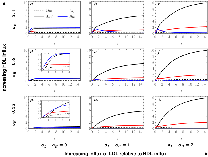
The numerical solutions suggest that plaque lipid content at equilibrium is more sensitive to the relative influx of LDL to HDL, $(\sigma_{L}-\sigma_{H})$, than to the individual influx rates $\sigma_{L}$ and $\sigma_{H}$. Indeed, when $\sigma_{L}-\sigma_{H}=2$ the trajectories of $A_{M}(t)$ and $L(t)$ are indistinguishable for $t\gtrapprox 4$ (see Fig.2, cases c,f,i). We note further that larger values of $(\sigma_{L}-\sigma_{H})$ give rise to larger increases in $A_{M}(t)$ than in $L(t)$ for the parameter values used in Figure 2. That is, increases to the relative influx of LDL to HDL yield greater changes in the macrophage lipid burden than the amount of extracellular lipid for these parameter values. These trends will be explored in more detail in Section 3.2.

The dynamics of the macrophage lipid distribution, $m_{j}(t)$, $j=0,1,\dots,J$, are shown in Figure 3. We see that, over time, $m_{j}(t)$ evolves in a wave-like manner towards a non-zero equilibrium. The wavefront proceeds from $j=0$ at $t=0$ to $j=j_{c}\in(0,J]$ as $t\rightarrow\infty$. We note, however, that the wavefront may change direction at later times (e.g. case a in Fig.3). This is likely due to offloading to HDL, given the dominance of $H(t)$ for these parameter values (see Fig.2a).

The lipid distribution $m_{j}$ adopts several qualitatively distinct profiles at equilibrium. The equilibrium profile may be monotone decreasing in $j$, and may be convex (as in case g) or concave (cases d and h); it may have a quasi-uniform profile (case e) or a peaked profile (cases a,b,c,f and i). The simulation results presented in Figure 3 suggest that the location of the wavefront at steady state is sensitive to the difference $(\sigma_{L}-\sigma_{H})$. However, the geometric features of the profile (e.g. existence of a local maximum) seem to depend on the individual magnitudes of $\sigma_{L}$ and $\sigma_{H}$. For instance, the spiked profile can manifest with low (e.g. case a), intermediate (e.g. case b) or high (e.g. case c) lipid loads. We study the equilibrium lipid distribution in more depth in Section 3.3.

Before proceeding to the steady state analysis, we pause to define two quantities which help to summarise the model behaviour:

Both variables are normalised such that $0\leq\mu(t),f(t)\leq 1$. The ratio $\mu(t)$ represents the average macrophage lipid burden, relative to the capacity for ingested lipid. Since

we note that another interpretation for $\mu$ is the fractional decrease in the phagocytosis rate of the macrophage population due to the lipid load at time $t$. The ratio $f(t)$ is the fraction of lipid in the lesion that is contained within the macrophage population.

The dynamics of $\mu(t)$ and $f(t)$ are shown in Figure 4 for $\sigma_{H}=1$ and $\sigma_{L}=0.75$, $1.5$, $3$, $6$ and $12$. Both variables tend to non-zero steady state values at long times: $\mu\rightarrow\mu^{\star}$ and $f\rightarrow f^{\star}$ as $t\rightarrow\infty$. We observe that as $\sigma_{L}$ increases, $\mu^{\star}$ increases towards $\mu^{\star}\rightarrow 1^{-}$, which corresponds to a plaque with macrophage lipid loads at capacity and, consequently, $100\%$ defective phagocytosis. By contrast, $f^{\star}$ depends non-monotonically on $\sigma_{L}$, attaining its largest value, $f^{\star}\approx 0.8$, when $1.5\lesssim\sigma_{L}\lesssim 3$. In order to understand these trends and those described above, we turn now to the steady state analysis.

Let $M^{\star}$, $A_{M}^{\star}$, $L^{\star}$ and $H^{\star}$ denote the steady values of the corresponding dependent variables. Expressions for these quantities can be found by setting the time derivatives to zero in equations (19)-(21). We find that $M^{\star}$, $A_{M}^{\star}$ and $H^{\star}$ can be expressed in term of $L^{\star}$:

and that $L^{\star}$ solves a quintic equation:

The coefficients $c_{i}$, $i=1,\dots,5$ are complicated combinations of the model parameters. Their expressions are given in Appendix A. We note that physically realistic steady state solutions must satisfy $A_{M}^{\star}\geq M^{\star}$ so that macrophage lipid content is not less than the endogenous lipid content. Re-writing this condition using the expressions for $A_{M}^{\star}$ and $M^{\star}$ in equations (28) supplies the following inequality for $L^{\star}$:

Hence, we seek positive solutions of the quintic (29) which satisfy inequality (30).

We used the Wolfram Mathematica routine NSolve to determine the positive solutions of equation (29) as $\sigma_{L}$ varies. The results, presented in Figure 5a, show that for fixed values of $\sigma_{L}$ polynomial (29) admits a unique physically realistic solution (with $L^{\star}\geq L^{\star}_{\text{min}}$). Further, $L^{\star}$ increases continuously with $\sigma_{L}$ and the solution branch can be decomposed into two main segments. On the left segment ($0\leq\sigma_{L}\lessapprox 0.8$ in Fig.5) $L^{\star}$ increases slowly with $\sigma_{L}$ and is well-approximated by $L^{\star}_{\text{min}}$. This regime corresponds to an HDL-dominant plaque where macrophage lipid loads are minimal ($A_{M}^{\star}\approx M^{\star}$) due to efficient offloading. In this regime, increasing LDL influx, $\sigma_{L}$, has little effect on extracellular lipid accumulation at equilibrium because macrophages rapidly offload the lipid they ingest and, therefore, only contribute their endogenous lipid content to the extracellular environment upon death. For large values of $\sigma_{L}$ ($\sigma_{L}\gtrapprox 0.8$ in Fig.5) $L^{\star}$ increases more rapidly with $\sigma_{L}$. For these plaques the LDL influx, $\sigma_{L}$, is sufficiently large to impact the quantity of unloaded HDL in the lesion at steady state.

While a closed-form expressions for $L^{\star}$ does not exist in full generality, we can approximate the individual segments of $L^{\star}$ via asymptotic analysis. Specifically, we seek approximate solutions to the polynomial (29) in the limit $\delta_{L}\sim\delta_{H}\ll 1$. Biologically, this corresponds to a regime in which loss of extracellular lipid and unloaded HDL to non-MDM interactions is negligible. It is possible to show that at leading order (see Appendix A), the coefficients scale as: $c_{0},\dots,c_{4}=\mathcal{O}(1)$ and $c_{5}=\mathcal{O}(\delta_{L},\delta_{H})$, so that equation (29) can be interpreted as a singular perturbation problem. We first consider the “outer" problem by setting $\delta_{L},\delta_{H}\rightarrow 0$ in equation (29). By factorising the resulting quartic polynomial into two quadratic equations for $L^{\star}$, we arrive at the following solutions:

where the constants $b_{0},b_{1}$ and $b_{2}$ of $L^{\star}_{2,\pm}$ are given by:

The remaining root is negative and scales as $L^{\star}_{0}=\mathcal{O}(\delta_{L}^{-1},\delta_{H}^{-1})$.

In Figure 5b we show how the solutions $L^{\star}_{1,+}$ and $L^{\star}_{2,+}$ change as $\sigma_{L}$ varies. We note that these expressions are good approximations for the left and right segments of $L^{\star}$ respectively. We note further that $L^{\star}_{\text{min}}$ reduces to $L^{\star}_{1,+}$ in the limit $\delta_{L}\rightarrow 0$, which indicates that $L^{\star}_{1,+}$ corresponds to a regime where $A_{M}^{\star}=M^{\star}+\mathcal{O}(\delta_{L},\delta_{H})$. Substituting this result into equations (28) shows that $H^{\star}=\mathcal{O}(\delta_{L}^{-1},\delta_{H}^{-1})$ at leading order, confirming that the slower increase with $\sigma_{L}$ on the left branch $L^{\star}_{1,+}$ is due to rapid offloading to HDL. The expression for $L^{\star}_{2,+}$ is more complicated and difficult to interpret. However, we note that the coefficients (33) which define $L^{\star}_{2,+}$ only depend on the influx parameters $\sigma_{L}$ and $\sigma_{H}$ through the combinations $\sigma_{L}-\sigma_{H}$ and $(1+\gamma)\sigma_{L}-\sigma_{H}$. This reinforces the notion that $L^{\star}$ is sensitive to the relative influx of LDL and HDL.

In Figure 6, we use the expressions (28) with the numerical solution for $L^{\star}$ in equation (29) to show how plaque composition at equilibrium changes as both $\sigma_{L}$ and $\sigma_{H}$ vary. We find that $M^{\star}$, $A_{M}^{\star}$ and $L^{\star}$ each increase with $\sigma_{L}$ and decrease with $\sigma_{H}$. By contrast, $H^{\star}$ decreases with $\sigma_{L}$ and increases with $\sigma_{H}$. We note that the approximately linear contours, which feature in all four plots, indicate that the dependent variables are sensitive to the difference $\sigma_{L}-\sigma_{H}$. This suggests that the relative influx of LDL lipid to HDL capacity not only determines $L^{\star}$ (as indicated by the asymptotics), but plaque composition more generally. When $\sigma_{L}-\sigma_{H}\lesssim 0$ (top left in plots of Fig.6), the plaque is HDL-dominant ($H^{\star}>25$) with low quantities of lipid ($A_{M}^{\star}$, $L^{\star}$) and a small macrophage population ($M^{\star}$). For $0\lesssim\sigma_{L}-\sigma_{H}\lesssim 5$ the plaque contains intermediate amounts of macrophages, lipid and HDL capacity. Finally, when $\sigma_{L}-\sigma_{H}\gtrsim 5$ the plaque is dominated by extracellular lipid ($L^{\star}>25$). In this regime, HDL capacity is exhausted ($H^{\star}\approx 0$) and macrophage lipid loads are near capacity ($A_{M}^{\star}\approx\kappa M^{\star}$) so that increases to the LDL lipid influx relative to HDL capacity, $(\sigma_{L}-\sigma_{H})$, directly increase the amount of extracellular lipid at steady state ($L^{\star}$).

We further explore plaque composition in Figure 7 where we focus on $\mu^{\star}$, the average macrophage lipid burden), $f^{\star}$, the fraction of lesion lipid that is intracellular and $A_{M}^{\star}+L^{\star}$, the total lesion lipid, as $\sigma_{L}$ and $\sigma_{H}$ vary. In contrast to the trends of $\mu^{\star}$ and $A_{M}^{\star}+L^{\star}$ (which both increase with $\sigma_{L}$ and decrease with $\sigma_{H}$), the fraction $f^{\star}$ exhibits non-monotonic dependence on both $\sigma_{L}$ and $\sigma_{H}$. It follows that $f^{\star}$ may be a poor metric for plaque progression since it can take the same value when plaque lipid content is low or high (e.g. $f^{\star}\approx 0.4$ at $(\sigma_{L},\sigma_{H})=(2,4)$ or $(6,2)$). We note further that $f^{\star}$ is approximately constant for $0\lesssim\sigma_{L}-\sigma_{H}\lesssim 5$, while $\mu^{\star}$ and $A_{M}^{\star}+L^{\star}$ vary substantially in this interval. This behaviour probably occurs because, in this region of parameter space, most of the lipid is contained in the macrophage population (compare plots for $A_{M}^{\star}$ and $L^{\star}$ in Fig.6), and so the primary source of extracellular lipid is cell death. Since the amount of lipid entering the extracellular environment via cell death is exactly the lipid content of the dying macrophages, cell death acts to equalise any changes in the amounts of intracellular and extracellular lipid. Finally, the plots confirm that the lesion is dominated by extracellular lipid in the region $\sigma_{L}-\sigma_{H}\gtrsim 5$, where macrophage lipid loads are comparable to the maximum lipid capacity.

It is not straightforward to analyse the lipid distribution $m_{j}(t)$, $j=0,1,\dots,J$ by directly considering equations (16)-(18). In Appendix B we show that closed-form solutions for the steady state values, $m_{j}^{\star}$, $j=0,1,\dots J$, can be obtained via the method of generating functions. The resulting steady state solutions read:

where $x^{(n)}=x(x+1)\cdots(x+n-1)$ is the $n$-th rising factorial of $x\in\mathbb{R}$, and $a_{c}$ and $p$ are the parameter groupings:

Although the solution (80) is exact, the complicated dependence of $m_{j}^{\star}$ on the index $j$ and the model parameters makes it difficult to analyse the geometric features of the distribution (e.g. the curvature, existence of a local maximum). We show below how this information can be readily extracted from a continuum approximation of equations (16)-(18).

References

- [1] M. Bäck, A. Yurdagul, I. Tabas, K. Öörni, P. T. Kovanen, Inflammation and its resolution in atherosclerosis: mediators and therapeutic opportunities, Nature Reviews Cardiology 16 (7) (2019) 389–406. doi:10.1038/s41569-019-0169-2.
- [2] I. Tabas, K. E. Bornfeldt, Macrophage phenotype and function in different stages of atherosclerosis, Circulation research 118 (4) (2016) 653–667. doi:10.1161/CIRCRESAHA.115.306256.
- [3] J. Boren, M. J. Chapman, R. M. Krauss, C. J. Packard, J. F. Bentzon, C. J. Binder, M. J. Daemen, L. L. Demer, R. A. Hegele, S. J. Nicholls, et al., Low-density lipoproteins cause atherosclerotic cardiovascular disease: pathophysiological, genetic, and therapeutic insights: a consensus statement from the european atherosclerosis society consensus panel, European heart journal 41 (24) (2020) 2313–2330. doi:10.1093/eurheartj/ehz962.
- [4] I. Razeghian-Jahromi, A. Karimi Akhormeh, M. Razmkhah, M. J. Zibaeenezhad, Immune system and atherosclerosis: Hostile or friendly relationship, International Journal of Immunopathology and Pharmacology 36 (2022) 03946320221092188. doi:10.1177/03946320221092188.
- [5] J. R. Guyton, K. F. Klemp, Development of the lipid-rich core in human atherosclerosis, Arteriosclerosis, thrombosis, and vascular biology 16 (1) (1996) 4–11. doi:10.1161/01.ATV.16.1.4.
- [6] M. Alique, C. Luna, J. Carracedo, R. Ramírez, Ldl biochemical modifications: a link between atherosclerosis and aging, Food & nutrition research 59 (1) (2015) 29240. doi:10.3402/fnr.v59.29240.
- [7] C. S. Zent, M. R. Elliott, Maxed out macs: physiologic cell clearance as a function of macrophage phagocytic capacity, The FEBS journal 284 (7) (2017) 1021–1039. doi:10.1111/febs.13961.
- [8] A. Remmerie, C. L. Scott, Macrophages and lipid metabolism, Cellular immunology 330 (2018) 27–42. doi:10.1016/j.cellimm.2018.01.020.
- [9] J. J. Pinney, F. Rivera-Escalera, C. C. Chu, H. E. Whitehead, K. R. VanDerMeid, A. M. Nelson, M. C. Barbeau, C. S. Zent, M. R. Elliott, Macrophage hypophagia as a mechanism of innate immune exhaustion in mab-induced cell clearance, Blood 136 (18) (2020) 2065–2079. doi:10.1182/blood.2020005571.
- [10] Y. Kojima, I. L. Weissman, N. J. Leeper, The role of efferocytosis in atherosclerosis, Circulation 135 (5) (2017) 476–489. doi:10.1161/CIRCULATIONAHA.116.025684.
- [11] A. Yurdagul Jr, A. C. Doran, B. Cai, G. Fredman, I. A. Tabas, Mechanisms and consequences of defective efferocytosis in atherosclerosis, Frontiers in cardiovascular medicine 4 (2018) 86. doi:10.3389/fcvm.2017.00086.
- [12] N. A. Avgerinos, P. Neofytou, Mathematical modelling and simulation of atherosclerosis formation and progress: a review, Annals of Biomedical Engineering 47 (8) (2019) 1764–1785. doi:10.1007/s10439-019-02268-3.
- [13] N. El Khatib, O. Kafi, A. Sequeira, S. Simakov, Y. Vassilevski, V. Volpert, Mathematical modelling of atherosclerosis, Mathematical modelling of natural phenomena 14 (6) (2019) 603. doi:10.1051/mmnp/2019050.
- [14] V. Calvez, A. Ebde, N. Meunier, A. Raoult, Mathematical modelling of the atherosclerotic plaque formation, in: Esaim: Proceedings, Vol. 28, EDP Sciences, 2009, pp. 1–12. doi:10.1051/proc/2009036.
- [15] A. D. Chalmers, C. A. Bursill, M. R. Myerscough, Nonlinear dynamics of early atherosclerotic plaque formation may determine the efficacy of high density lipoproteins (hdl) in plaque regression, PLoS One 12 (11) (2017) e0187674. doi:10.1371/journal.pone.0187674.
- [16] T. Silva, W. Jäger, M. Neuss-Radu, A. Sequeira, Modeling of the early stage of atherosclerosis with emphasis on the regulation of the endothelial permeability, Journal of Theoretical Biology 496 (2020) 110229. doi:10.1016/j.jtbi.2020.110229.
- [17] H. Z. Ford, H. M. Byrne, M. R. Myerscough, A lipid-structured model for macrophage populations in atherosclerotic plaques, Journal of Theoretical Biology 479 (2019) 48–63. doi:10.1016/j.jtbi.2019.07.003.
- [18] K. L. Chambers, M. G. Watson, M. R. Myerscough, A lipid-structured mathematical model of atherosclerosis with macrophage proliferation, arXiv preprint arXiv:2205.04715 (2022). doi:10.48550/arXiv.2205.04715.
- [19] M. G. Watson, K. L. Chambers, M. R. Myerscough, A lipid-structured model of atherosclerotic plaque macrophages with lipid-dependent kinetics, arXiv preprint arXiv:2205.05285 (2022). doi:10.48550/arXiv.2205.05285.
- [20] N. Meunier, N. Muller, Mathematical study of an inflammatory model for atherosclerosis: a nonlinear renewal equation, Acta Applicandae Mathematicae 161 (1) (2019) 107–126. doi:10.1007/s10440-018-0206-x.
- [21] J. W. Williams, K. Zaitsev, K.-W. Kim, S. Ivanov, B. T. Saunders, P. R. Schrank, K. Kim, A. Elvington, S. H. Kim, C. G. Tucker, et al., Limited proliferation capacity of aortic intima resident macrophages requires monocyte recruitment for atherosclerotic plaque progression, Nature immunology 21 (10) (2020) 1194–1204. doi:10.1038/s41590-020-0768-4.
- [22] H. Z. Ford, L. Zeboudj, G. S. Purvis, A. Ten Bokum, A. E. Zarebski, J. A. Bull, H. M. Byrne, M. R. Myerscough, D. R. Greaves, Efferocytosis perpetuates substance accumulation inside macrophage populations, Proceedings of the Royal Society B 286 (1904) (2019) 20190730. doi:10.1098/rspb.2019.0730.
- [23] N. Taefehshokr, C. Yin, B. Heit, Rab gtpases in the differential processing of phagocytosed pathogens versus efferocytosed apoptotic cells, Histol. Histopathol 36 (2021) 123–135. doi:10.14670/HH-18-252.
- [24] J. Westman, S. Grinstein, P. E. Marques, Phagocytosis of necrotic debris at sites of injury and inflammation, Frontiers in immunology 10 (2020) 3030. doi:10.3389/fimmu.2019.03030.
- [25] M. P. Thon, H. Z. Ford, M. W. Gee, M. R. Myerscough, A quantitative model of early atherosclerotic plaques parameterized using in vitro experiments, Bulletin of mathematical biology 80 (1) (2018) 175–214. doi:10.1007/s11538-017-0367-1.
- [26] T. A. Angelovich, A. C. Hearps, A. Maisa, T. Kelesidis, A. Jaworowski, Quantification of monocyte transmigration and foam cell formation from individuals with chronic inflammatory conditions, JoVE (Journal of Visualized Experiments) (2017) e56293doi:10.3791/56293.
- [27] A. Ghattas, H. R. Griffiths, A. Devitt, G. Y. Lip, E. Shantsila, Monocytes in coronary artery disease and atherosclerosis: where are we now?, Journal of the American College of Cardiology 62 (17) (2013) 1541–1551. doi:10.1016/j.jacc.2013.07.043.
- [28] E. Bruckert, D. Rosenbaum, Lowering ldl-cholesterol through diet: potential role in the statin era, Current opinion in lipidology 22 (1) (2011) 43–48. doi:10.1097/MOL.0b013e328340b8e7.
- [29] Kummer confluent hypergeometric function, https://functions.wolfram.com/HypergeometricFunctions/Hypergeometric1F1/.
- [30] Hermite hypergeometric function, https://functions.wolfram.com/HypergeometricFunctions/HermiteHGeneral/.
- [31] Y. Ge, M. Huang, Y.-m. Yao, Efferocytosis and its role in inflammatory disorders, Frontiers in Cell and Developmental Biology 10 (2022). doi:10.3389/fcell.2022.839248.
- [32] C. Yin, B. Heit, Cellular responses to the efferocytosis of apoptotic cells, Frontiers in Immunology 12 (2021) 631714. doi:10.3389/fimmu.2021.631714.
- [33] L. Chen, J. Zhang, X. Yang, Y. Liu, X. Deng, C. Yu, Lysophosphatidic acid decreased macrophage foam cell migration correlated with downregulation of fucosyltransferase 8 via hnf1, Atherosclerosis 290 (2019) 19–30. doi:10.1016/j.atherosclerosis.2019.09.001.
- [34] C. S. Robbins, I. Hilgendorf, G. F. Weber, I. Theurl, Y. Iwamoto, J.-L. Figueiredo, R. Gorbatov, G. K. Sukhova, L. Gerhardt, D. Smyth, et al., Local proliferation dominates lesional macrophage accumulation in atherosclerosis, Nature medicine 19 (9) (2013) 1166–1172. doi:10.1038/nm.3258.
- [35] G. L. Celora, H. M. Byrne, P. Kevrekidis, Spatio-temporal modelling of phenotypic heterogeneity in tumour tissues and its impact on radiotherapy treatment, Journal of Theoretical Biology 556 (2023) 111248. doi:10.1016/j.jtbi.2022.111248.
- [36] G. Fiandaca, S. Bernardi, M. Scianna, M. E. Delitala, A phenotype-structured model to reproduce the avascular growth of a tumor and its interaction with the surrounding environment, Journal of Theoretical Biology 535 (2022) 110980. doi:10.1016/j.jtbi.2021.110980.
- [37] K. Kim, D. Shim, J. S. Lee, K. Zaitsev, J. W. Williams, K.-W. Kim, M.-Y. Jang, H. Seok Jang, T. J. Yun, S. H. Lee, et al., Transcriptome analysis reveals nonfoamy rather than foamy plaque macrophages are proinflammatory in atherosclerotic murine models, Circulation research 123 (10) (2018) 1127–1142. doi:10.1161/CIRCRESAHA.118.312804.