Search for planets around stars with wide brown dwarfs
Abstract
Aims. The project aims to understand better the role of wide brown dwarf companions on planetary systems.
Methods. We obtained high-resolution spectra of six bright stars with co-moving wide substellar companions with the SONG, CARMENES, and STELLA high-resolution spectrographs. We used these spectra to derive radial velocities together with a complete set of stellar physical parameters. We then investigated radial velocities signals and discussed the fraction of planets in such systems. We also re-analyzed the ages of our targets, which were used to derive the physical parameters of wide brown dwarf companions. Finally, a compilation of systems with known planets from the literature is considered along with our sample to search for possible peculiarities in their parameter distributions.
Results. Based on the derived ages of six observed systems, we re-computed the masses of the wide companions, confirming their substellar nature. We confirmed planets in the HD 3651 and HIP 70849 systems and found a new planetary candidate in the HD 46588 system. In our survey, which is sensitive mostly to Neptune-mass planets at short periods of a few days and Saturn-mass planets at longer periods of hundreds of days, we derived a frequency of planets orbiting stars with wide brown dwarf companions below 70% with the uncertainties included. Comparing the parameter distributions of our sample with single stars, we observe the enhancement of planets with short periods below six days in systems with a wide stellar companion. Finally, planets in systems with wide BD companions follow their own eccentricity distribution with a maximum at and have periods larger than 40 days, masses larger than , and eccentricities larger than 0.4.
Key Words.
BDs – planetary systems – spectroscopy – radial velocity – stellar ages stars (individual): GJ 504, HD 3651, HD46588, HD203030, HN Peg, HD1188651 Introduction
Thousands of brown dwarfs (BDs) have been discovered so far; many come from all-sky infrared surveys (Martín et al. 1999; Tsvetanov et al. 2000; Cruz et al. 2007; Lodieu et al. 2007; Kirkpatrick et al. 2011; Lodieu et al. 2012; Deacon et al. 2014; Carnero Rosell et al. 2019, e.g.,), such as the Two-Micron All-Sky Survey (Skrutskie et al. 2006, 2MASS;), the Wide-field Infrared Survey Explorer (Wright et al. 2010, WISE;), the Deep Near-Infrared Survey of the Southern Sky (Epchtein et al. 1997, DENIS;), the UKIRT Infrared Deep Sky Survey (Lawrence et al. 2007, UKIDSS;), and the VISTA Hemisphere Survey (McMahon et al. 2013, VHS;). Additional discoveries come from large-scale optical surveys, such as the Dark Energy Survey (Abbott et al. 2018, DES;), the Sloan Digital Sky Survey (York et al. 2000, SDSS;), and the Panoramic Survey Telescope and Rapid Response System (Chambers et al. 2016, Pan-STARRS;).
Most of the discovered BDs are free-floating. Only a small fraction of them are confirmed as wide co-moving companions to stars (Deacon et al. 2014). However, the recent study by dal Ponte et al. 2020 provides almost 300 new candidate co-moving BDs using data from the Dark Energy Survey DR1 and DR2 (Gaia Collaboration et al. 2018b). dal Ponte et al. 2020 observed a wide binary fraction of BDs about 2–4% over most of the spectral types (L0–T8.5), more significantly for L dwarf companions with better statistics. We should also mention the rising group of transiting BDs (Persson et al. 2019; Šubjak et al. 2020; Carmichael et al. 2020; Carmichael et al. 2021; Palle et al. 2021, e.g.,) discovered lately mainly thanks to the space missions such as the CoRoT mission (Auvergne et al. 2009), the Kepler/K2 mission (Borucki et al. 2010), and currently the TESS mission (Ricker et al. 2015). The updated list of known transiting BDs can be found in Šubjak et al. 2020. BDs can be commonly found also in binaries. Tens of them are listed in Liu et al. 2010. Even two unique young systems with BDs in an eclipsing binary were reported by Stassun et al. 2006 and Triaud et al. 2020. Another unique structure has systems of two BDs orbiting a primary star, such as HIP 73990 (Hinkley et al. 2015) and Oph (Quirrenbach et al. 2019). We can hence find BDs in systems with different structures, which create opportunities to study different kinds of processes and interactions.
From this point of view are particularly interesting systems with wide BD companions around planet-host stars. To date, only nine such systems have been reported. If the mass of a companion is close to the stellar/substellar boundary, we include only a companion confirmed as a brown dwarf based on spectroscopic observations. The confirmed systems are: HD 3651 (Fischer et al. 2003; Mugrauer et al. 2006; Luhman et al. 2007; Burgasser 2007; Brewer et al. 2020, e.g.,), HIP 70849 (Ségransan et al. 2011; Lodieu et al. 2014), HD 168443 (Marcy et al. 2001; Pilyavsky et al. 2011), HD 65216 (Mayor et al. 2004; Mugrauer et al. 2007), HD 89744 (Korzennik et al. 2000; Mugrauer et al. 2004), HD 4113 (Tamuz et al. 2008; Ednie et al. 2018; Cheetham et al. 2018), GJ 229 (Geißler et al. 2008; Tuomi et al. 2014; Feng et al. 2020), HD 41004 (Santos et al. 2002; Zucker et al. 2003; Zucker et al. 2004), and Indi (Scholz et al. 2003; McCaughrean et al. 2004; Feng et al. 2019). However, HD 65216, HD 41004 and Indi have different architectures (see Appendix C).
Planets can be significantly affected by wide BD companions through different processes, such as gravitational instability, accretion, velocities of colliding planetesimals, dissipation, or Lidov-Kozai effects (Boss 2006; Nelson 2003; Moriwaki & Nakagawa 2004, e.g.,). If we look at multiple stellar systems with planets, possible peculiarities in parameter distributions of inner planets were searched by many teams (Butler et al. 1997; Mugrauer et al. 2005; Desidera & Barbieri 2007; Bonavita & Desidera 2007, e.g.,). Among them, we can highlight the peculiarities in the mass-period and eccentricity-period distributions (Eggenberger et al. 2004; Zucker & Mazeh 2002, e.g.,). Such peculiarities reflect the interaction between inner planets and wide companions, placing constraints on various scenarios proposed for their formation and evolution (Eggenberger et al. 2004). Thus, it is reasonable to search for peculiarities in systems with wide BD companions hosting planets.
The systems with wide BD companions and planets offer great potential and opportunities to enrich our knowledge about both groups of objects and test our planetary formation and evolution concepts. A large sample of such systems is needed to reveal possible peculiarities and provide a detailed discussion. It leads to fundamental questions like: What is the fraction of systems with wide BD companions that host planets? Are they common, or is there any process that disfavors this scenario? In this paper, we focus on a sub-sample of six stars with confirmed co-moving wide BD companions using high-resolution spectroscopic data. These systems are GJ 504 (Kuzuhara et al. 2013), HD 46588 (Loutrel et al. 2011), HD 203030 (Metchev & Hillenbrand 2006), HD 3651 (Mugrauer et al. 2006), HN Peg (Luhman et al. 2007), and HD 118865 (Burningham et al. 2013). We describe the target selection process in Section 2. We present new observations in Section 3 and make use of archival datasets described in Section 4. We derive the physical parameters of our targets in Section 5 and investigate the nature of radial velocity (RV) signals to search for planets in Section 6. In Section 7 we compare the sample of systems with confirmed planets and wide BD companions previously published in the literature with single planet-host-stars and planet-host-stars with wide stellar companions to discuss possible peculiarities in their parameter distributions. Finally, we summarize final conclusions in Section 8.
2 Target justification
Following the discovery of a T4.5 dwarf companion at 6.3′ (9000 au) from HIP 70849 (Lodieu et al. 2014), a K7V star which hosts a 9 MJup planet with an eccentric orbit (Ségransan et al. 2011), we searched the literature for other wide co-moving systems with one substellar component and a bright ( 6 mag) host suitable for intensive spectroscopic follow-up with the 1-m robotic Stellar Observations Network Group (SONG) telescope (Fredslund Andersen et al. 2019). Among the brightest primaries of wide substellar companions visible from the Northern hemisphere, we recovered HD 3651 (Mugrauer et al. 2006). The other targets suitable for our project were at that time: HD 46588 (Loutrel et al. 2011), HN Peg (Luhman et al. 2007), GJ 504 (Kuzuhara et al. 2013; Janson et al. 2013; Skemer et al. 2016). We subsequently added HD 203030 (Metchev & Hillenbrand 2006) when the magnitude limit of the SONG guiding was increased to = 8.5 mag as well as HD 118865 (Burningham et al. 2013) to gauge the performance of the STELLar Activity (STELLA) 1.2-m robotic telescopes (Strassmeier et al. 2004). These six sources constituted our sample when we started the project in 2015. The parameters of the observed sample of stars are listed in Table 1. We emphasize that the population of wide L and T dwarf companions has increased significantly over the past decade, as compiled in Deacon et al. 2012 and dal Ponte et al. 2020. Hence, this work can be considered as a pilot program and the statistical results should be considered as preliminary.
| System | GJ 504 | HD 3651 | HD 46588 | HD 203030 | HN Peg | HD 118865 | Source |
| RAJ2000 (hh:mm:ss.ss) | 13 16 46.52 | 00 39 21.81 | 06 46 14.15 | 21 18 58.22 | 21 44 31.33 | 13 39 34.33 | 2 |
| DecJ2000 (d:’:”) | 09 25 26.97 | 21 15 01.72 | 79 33 53.32 | 26 13 49.96 | 14 46 18.98 | 01 05 18.13 | 2 |
| TESS mag | 3 | ||||||
| mag | 1 | ||||||
| Tycho mag | 4 | ||||||
| Tycho mag | 4 | ||||||
| 2MASS mag | 5 | ||||||
| 2MASS mag | 5 | ||||||
| 2MASS mag | 5 | ||||||
| WISE1 mag | 6 | ||||||
| WISE2 mag | 6 | ||||||
| WISE3 mag | 6 | ||||||
| WISE4 mag | 6 | ||||||
| (mas/yr) | 1 | ||||||
| (mas/yr) | 1 | ||||||
| Parallax (mas) | 1 |
References: 1 - eDR3, Gaia Collaboration et al. 2021; 2 - DR2, Gaia Collaboration et al. 2018b;
3 - TESS, Stassun et al. 2018; 4 - Tycho, Høg et al. 2000; 5 - 2MASS, Cutri et al. 2003; 6 - WISE, Wright et al. 2010
3 Spectroscopic observations
We performed high-resolution spectroscopy with several telescopes and instruments whose observations are described below.
3.1 SONG spectroscopy
We observed our sample of stars with the robotic Stellar Observations Network Group (SONG) Hertzsprung telescope (Fredslund Andersen et al. 2019) through a dedicated program with nightly observations when weather permitted for two years ( 4 semesters) in most cases. The time interval of the observations, together with the number of acquired spectra, are reported in Table 2. We used the slit of 1.2 arcsec, yielding a spectral resolution of 90,000. To ensure sufficient count over the full wavelength range of SONG spectra, we employed exposure times between 360 and 600s, leading to a signal-to-noise ratio of at least 50 per resolution element for all observations. The numbers of gathered spectra for each system, together with the range of dates of observations, are in Table 2.
SONG is a 1–m telescope located in the Observatorio del Teide in Tenerife, Canary Islands. It is equipped with a high-resolution echelle spectrograph operating in the visible band between 440 and 690 nm with an average dispersion of 0.002 nm/pixel. The detector is an Ikon-L commercial charged-coupled device camera developed by Andor with a 2k2k chip size. The SONG spectra and the RVs have been kindly provided by the SONG team as derived by the iSONG software (Antoci et al. 2013) following the procedure described in (Grundahl et al. 2017).
3.2 Calar Alto/CARMENES spectroscopy
We collected visible and near-infrared spectra for each system with the Calar Alto high-resolution search for M dwarfs with Exoearths with Near-infrared and optical Echelle Spectrographs (Quirrenbach et al. 2014, CARMENES;). The time interval of the observations, together with the number of acquired spectra, are reported in Table 2. All observations were conducted in queue mode by the staff of the Calar Alto observatory, satisfying the requested conditions: seeing better than two arcsec and clear skies. We set the exposure times between 250-900 seconds depending on the star’s brightness, targeting the minimum signal-to-noise ratio (S/N) of 150 based on the estimates of the exposure time calculator.
CARMENES consists of two independent high-resolution echelle spectrographs in the visible (520–960 nm; R = 93,400) and near-infrared (960–1710 nm; R = 81,800) which are simultaneously fed through fibres.
The data were reduced using CARACAL (Caballero et al. 2016), and the visible and near-infrared radial velocities were obtained with SERVAL (Zechmeister et al. 2018). SERVAL determines radial velocity by co-adding all available spectra of the target with an S/N higher than 10 and creating a high-quality template of the star used as a reference spectrum. The radial velocities were corrected for barycentric motion, secular perspective acceleration, instrumental drift, and nightly zero points (Trifonov et al. 2018).
3.3 STELLA spectroscopy
We observed HD 118865 system with the STELLar Activity (STELLA) two 1.2-m robotic telescopes located at Izaña Observatory in Tenerife (Strassmeier et al. 2004). The fibre-fed Echelle Spectrograph of STELLA with an e2v 2k2k CCD detector covers the wavelength range between 390–880 nm and has the resolving power of R = 55,000. The spectra were automatically reduced using the IRAF-based STELLA data-reduction pipeline (Weber et al. 2008), and RVs were kindly provided by the STELLA team. The time interval of the observations, together with the number of acquired spectra, are reported in Table 2.
| Star | # spectra | Date |
| SONG spectrograph | ||
| GJ 504 | 262 | 2016-Feb-7 to 2017-Aug-19 |
| HD 3651 | 414 | 2014-Sep-03 to 2016-Feb-14 |
| HD 46588 | 352 | 2015-Apr-3 to 2017-Mar-6 |
| HD 203030 | 111 | 2017-Apr-17 to 2018-Sep-29 |
| HN Peg | 250 | 2015-Apr-22 to 2017-Jan-15 |
| CARMENES spectrograph | ||
| GJ 504 | 39 | 2019-Jan-04 to 2019-Jun-28 |
| HD 3651 | 19 | 2019-Jan-03 to 2019-Jun-29 |
| HD 46588 | 35 | 2019-Jan-04 to 2019-May-25 |
| HD 203030 | 32 | 2019-Jan-03 to 2019-Jun-29 |
| HN Peg | 25 | 2019-Jan-03 to 2019-Jun-29 |
| HD 118865 | 54 | 2019-Jan-04 to 2019-Jun-28 |
| STELLA spectrograph | ||
| HD 118865 | 101 | 2017-Feb-01 to 2017-Jul-29 |
| Archival data | ||
| GJ 504 | ||
| SOPHIE | 38 | 2013-Apr-01 to 2016-May-23 |
| Lick | 57 | 1987-Jun-12 to 2009-Feb-2 |
| HARPS-N | 106 | 2016-Jun-9 to 2018-Apr-1 |
| HD 3651 | ||
| EXPRES | 61 | 2019-Aug-18 to 2020-Feb-1 |
| HIRES | 161 | 1996-Oct-10 to 2013-Dec-14 |
| LICK | 155 | 1987-Sep-9 to 2011-Oct-12 |
| HRS | 35 | 2005-Jul-29 to 2007-Nov-19 |
| Tull | 4 | 2005-Sep-20 to 2006-Oct-12 |
| HD 203030 | ||
| HIRES | 17 | 2002-Aug-28 to 2013-Aug-26 |
| HN Peg | ||
| LICK | 37 | 1987-Sep-9 to 2004-Aug-2 |
| HARPS | 22 | 2013-Oct-10 to 2017-Jun-3 |
4 Supporting observational data
We searched for archival spectroscopic observations, which we used as supplemental data in our analyses. In addition, we also downloaded photometric data from the Transiting Exoplanet Survey Satellite (TESS) (Ricker et al. 2015) available for the stars from our sample.
4.1 Archival spectroscopy
GJ 504, HD 3651, HN Peg and HD 203030 are systems that were already observed spectroscopically. We downloaded public archival data to complement our own observational datasets.
For GJ 504, we checked the HARPS-N archive and noticed that additional spectra had been collected with the HARPS-N (Cosentino et al. 2012) by the GAPS team between 9 June 2016 and 01 April 2018, amounting to a total of 106 spectra. We re-processed all HARPS-N spectra with the SERVAL pipeline to get RV measurements and activity indicators. Additionally, we found 58 spectra (Fischer et al. 2014) collected with the LICK spectrograph (Vogt 1987); however, their relatively low cadence over the long baseline do not make them very useful as the star shows a high level of activity (we do not see any significant signal in the periodograms). For the same reason, we did not use 38 RVs (Bonnefoy et al. 2018) collected with the SOPHIE spectrograph (Bouchy & Sophie Team 2006). In their periodogram, we only see peaks close to the rotation period of the stars visible in all used datasets.
For HD 3651, we also used RVs published in Brewer et al. 2020. These authors report 61 spectra from the EXPRES spectrograph (Jurgenson et al. 2016) mounted on the 4.3-m Lowell Observatory Discovery Channel Telescope (DCT). We also included an additional 161 archival Keck HIRES data (Vogt et al. 1994) with the 17-year time baseline (Butler et al. 2017), 155 archival LICK RVs (Fischer et al. 2014), 35 archival RVs obtained with the High Resolution Spectrograph (HRS) (Tull 1998) mounted at the 9.2m Hobby–Eberly Telescope (HET) (Wittenmyer et al. 2009), and four archival RVs obtained with the Tull spectrograph (Tull et al. 1995) at the 2.7m Harlan J.Smith Telescope (Wittenmyer et al. 2009).
For HD 203030, we found 17 Keck HIRES RVs (Butler et al. 2017). However, with the 17-year time baseline and the star’s level of activity, these data are not helpful, and we do not observe any significant signal in the periodogram.
Finally, for HN Peg, we found 37 LICK RVs (Fischer et al. 2014) and 22 HARPS RVs. However, because of the RV scatter caused by the stellar activity, such small datasets are also not helpful compared to the SONG dataset. The complete list of available archival data is reported in Table 2.

4.2 TESS photometry
TESS observed each of our targets except HN Peg at least in one sector at a two-minute cadence mode during its prime mission. The full list of observations is summarized in Table 3. We used the lightkurve package in Python (Lightkurve Collaboration et al. 2018) to download TESS target pixel files from the Mikulski Archive for Space Telescopes (MAST)11 1 https://mast.stsci.edu/portal/Mashup/Clients/Mast/Portal.html. We then selected optimal aperture masks to extract light curves (LCs) for each system, which we corrected for outliers and normalized. On them, we performed the Pixel Level Decorrelation method (Deming et al. 2015) to remove systematics. The final TESS LCs are shown in the middle of Fig. 1. None of our targets is recognized as TESS Object of Interest (TOI), meaning that no obvious transit-like feature has been identified in the LCs.
We used Tpfplotter (Aller et al. 2020) to overplot the DR2 catalogue to the TESS target pixel file (tpf) to investigate possible diluting sources in TESS photometry with the limiting difference in magnitude of 10. Tpf images for our sample of stars created with tpfplotter can be seen on the left-hand side of Fig. 1. There is only one additional source between TESS pixels used in SAP in the case of GJ 504. This star has identification ID 3732539649257672704 and magnitude of 14. According to colour bands, we classify this object as K7–K9 spectral type, with mag corresponding to K8–K9, and mag corresponding to K7--K8. To compute the spectral type we used the up-to-date version22 2 https://www.pas.rochester.edu/~emamajek/EEM_dwarf_UBVIJHK_colors_Teff.txt of the dwarf color sequence from Pecaut & Mamajek 2013. For HD 203030, there are five additional sources within the aperture of the TESS pixels. The full list of these sources with relevant information is displayed in Table 4. We conclude that these sources are too faint compared to GJ 504, HD 203030, respectively, to yield any significant dilution. We did not find any diluting sources in the TESS apertures for the rest of the systems in our sample.
| Star | Sector | Date |
|---|---|---|
| GJ 504 | 23 | 2020-Mar-20 to 2020-Apr-15 |
| 50 | 2022-Mar-26 to 2022-Apr-22 | |
| HD 3651 | 17 | 2019-OCt-7 to 2019-Nov-2 |
| HD 46588 | 19 | 2019-Nov-27 to 2019-Dec-24 |
| 20 | 2019-Dec-24 to 2020-Jan-21 | |
| 26 | 2020-Jun-08 to 2020-Jul-04 | |
| 40 | 2021-Jun-24 to 2021-Jul-23 | |
| 47 | 2021-Dec-30 to 2022-Jan-28 | |
| 53 | 2022-Jun-13 to 2022-Jul-09 | |
| HD 203030 | 15 | 2019-Aug-15 to 2019-Sep-11 |
| 55 | 2022-Aug-5 to 2022-Sep-1 | |
| HD 118865 | 23 | 2020-Mar-18 to 2019-Apr-16 |
| 45 | 2021-Dec-02 to 2021-Dec-30 | |
| 50 | 2022-Mar-26 to 2022-Apr-22 | |
| HN Peg | 55 | 2022-Aug-5 to 2022-Sep-1 |
| ID | mag | Spectral type | close to |
|---|---|---|---|
| 3732539649257672704 | 14.0 | K7–9 | GJ 504 |
| 1846882426008946304 | 15.2 | K3–4/K5–6 | HD 203030 |
| 1846882219850515968 | 17.2 | K1–3 | HD 203030 |
| 1846882430304186112 | 15.6 | G9–K0 | HD 203030 |
| 1846882533383405696 | 17.7 | K4–6 | HD 203030 |
| 1846882322929096704 | 18.1 | K3–4 | HD 203030 |
5 Stellar and brown dwarf parameters
In this section, we derive the stellar parameters of stars in our sample as well as the ages of individual systems, which are then used to infer the ages of wide companions and derive their parameters. We need to know the parameters of the host stars if we want to derive parameters of potential planets, and if we want later discuss peculiarities in the parameter distributions of these planets, it is crucial to describe every known object in these systems. We have done this for all studied systems regardless of whether we found any planetary candidate.
5.1 Stellar parameters with iSpec and VOSA
We used the iSpec framework (Blanco-Cuaresma et al. 2014; Blanco-Cuaresma 2019) to derive the parameters of the host stars from the co-added CARMENES spectra. iSpec determines stellar parameters by minimalization of the value between the calculated synthetic spectrum and observed spectrum. To determine the effective temperature , metallicity , surface gravity , and the projected stellar equatorial velocity we followed the same procedure as in Fridlund et al. 2017. The whole procedure is described in detail in Appendix A.1, and we report the stellar parameters for the stars of our sample in Table 5.
As a sanity check, we also analyzed the spectral energy distribution with the Virtual Observatory SED Analyser (Bayo et al. 2008, VOSA33 3 http://svo2.cab.inta-csic.es/theory/vosa/;). VOSA performs the minimization procedure to compare theoretical models with the observed photometry. For our SED fitting, we use the Strömgren-Crawford uvby (Paunzen 2015), Tycho (Høg et al. 2000), DR2 (Gaia Collaboration et al. 2018b), eDR3 (Gaia Collaboration et al. 2021), 2MASS (Cutri et al. 2003), AKARI (Ishihara et al. 2010), and WISE (Cutri et al. 2021) photometry. The whole procedure is described in detail in Appendix A.2, and we report the stellar parameters for the stars of our sample in Table 5.
| System | GJ 504 | HD 3651 | HD 46588 | HD 203030 | HN Peg | HD 118865 |
|---|---|---|---|---|---|---|
| iSpec & PARAM 1.5 analysis | ||||||
| (km/s) | ||||||
| (Å) | 0.087 | ¡0.010 | 0.051 | 0.050 | 0.103 | 0.076 |
| () | ||||||
| () | ||||||
| (days) | 4.59–5.17 (7) | |||||
| VOSA analysis | ||||||
| 5900–6200 | 5200–5400 | 6100–6300 | 5400–5600 | 5900–6100 | 6000–6200 | |
| 0.0–0.5 | 0.0–0.5 | 0.0–0.5 | 0.0–0.5 | –0.5 | 0.0–0.5 | |
| 4–5 | 4–5 | 4–5 | 4–5 | 4–5 | 4–5 | |
| () | 1.25–1.40 | 0.81–0.89 | 1.12–1.21 | 0.81–0.88 | 0.94–1.03 | 1.19–1.29 |
| () | 2.05–2.16 | 0.50–0.54 | 1.77–1.92 | 0.57–0.60 | 1.11–1.20 | 1.89–2.02 |
| Sp. type | G0V (1) | K0V (2) | F8V (3) | G8V (4) | G0V (5) | F7V (6) |
| (W) | 22.5 (8) | 20.2 (8) | 21.0 (8) | 21.8 (8) | 22.2 (8) | — |
References: (1) - Anderson et al. 2010, (2) - Keenan & McNeil 1989, (3) - Abt 2009, (4) - Frasca et al. 2018
(5) - Gray et al. 2001, (6) - Houk & Swift 1999, (7) - Messina & Guinan 2003, (8) - Voges et al. 1999
5.2 Analysing the surface rotation
To determine the rotation period from the TESS light curves (LCs), we apply generalised Lomb-Scargle (GLS) periodograms (Zechmeister & Kürster 2009) investigating the most dominant signals. Plots of periodograms for individual stars can be found in Fig. 1. GJ 504 and HD 203030 show clear variations with the periods of 3.4 days and 6.7 days, respectively, which we interpret as the rotation periods. HD 3651 does not show clear variations but only a long trend; hence we interpret the rotation period to be larger than the TESS data baseline. It is consistent with the period of 44.5 days derived through the calibration from the value of log by Fischer et al. 2003. Brewer et al. 2020 then searched for photometric variations using 1192 photometric observations collected over the period of 25 yr with the 0.75m Automatic Photoelectric Telescope (APT) at Fairborn Observatory in southern Arizona. However, they did not find any significant variability within any observing season. Finally, after we removed long trends in the HD 46588 and HD 118865 datasets, we could identify variations with the periods of 10.3 days and 6.2 days that we interpret as the rotation periods. The variations in the HD 118865 LC are not so clear as for other objects; however, we used this period only to derive the bottom limit for the age, as can be seen in the next section. We did not find any contradictions with rotation periods reported in the literature. For example, in the catalogue of rotation periods by Wright et al. 2011 we can see the rotation period of 6.67 d for HD 203030, 4.86 d for HN Peg and 48 d for HD 3651. Donahue et al. 1996 then reported the rotation period of 3.33 d for GJ 504.
5.3 Age analysis
To determine the age of the sample stars, we provide an extensive analysis of several complementary age indicators. We include stellar isochrones fitting, gyrochronology analysis, lithium equivalent width, X-ray luminosity, and membership to young associations. Our effort is to examine each age indicator separately to provide the age intervals for each of them and to determine the final age as an overlap between these intervals. Detailed description of each age indicator can be found in Appendix B and the results are listed in Table 6.
We found that all age indicators for our sample of stars are quite consistent with each other. Two inconsistencies are that the gyrochronology predicts a slightly lower age of HD 203030 and the isochrone fitting for the GJ 504, HD 203030 and HD 46588 gives older ages than the rest of the indicators. However, we found agreement in most cases when considering 95% confidence intervals from isochrone fitting. The GJ 504 age is intensively discussed in the literature. Kuzuhara et al. 2013 estimated the age of GJ 504 to be Myr using gyrochronology and chromosphere activity of the star. Fuhrmann & Chini 2015; D’Orazi et al. 2017 have found that the isochrones comparison suggests an older age between 1.8 and 3.5 Gyr. Authors speculated that the recent merging of hot Jupiter companion could explain the star’s high activity level. Bonnefoy et al. 2018 have recently revisited the system parameters. Instead of using an effective temperature as an input to isochrone fitting, they used an interferometric radius of for GJ 504. However, the fact that we got, as an output from isochrone fitting, the radius with similar uncertainty as these authors measured suggests that both analyses should be equivalent in terms of age determination. They found two isochronal age scenarios: the young one with an age of Myr and the old one with an age of Gyr.

We confirm that most age indicators lead toward the relatively young age of several hundred Myr. Similarly to Bonnefoy et al. 2018, we also found that isochrone fitting gives two possible age scenarios. It can be seen in Figure 2, where we plot GJ 504’s luminosity from the SED analysis and effective temperature, together with the MIST stellar evolutionary tracks (Choi et al. 2016). We also note that the age depends on the isochrone model used. Using the PARSEC isochrones (Bressan et al. 2012) we found the age of Gyr, while for the MIST isochrones we found Gyr. Similarly to other stars in our sample, in Table 6 we provide an age for GJ 504 as an overlap of most of the activity indicators. However, we do not consider this age final, and we are open to both younger and older scenarios. That’s why we keep this system in or sample as a system with the potential wide BD companion.
If we consider that BDs cool down with age, their detection becomes more challenging as they get older. In this context, it is not surprising that a lot of the stars in our sample are relatively young, i.e. 1 Gyr or lower. Nonetheless, we found few systems older than 2.5 Gyr.
| System age (Gyr) | GJ 504 | HD 3651 | HD 46588 | HD 203030 | HN Peg | HD 118865 |
|---|---|---|---|---|---|---|
| Isochrones | ||||||
| Gyrochronology | 0.12–0.55 | 2.5 | 0.8–2.5 | 0.35–0.55 | 0.35–0.65 | 0.60–1.2 |
| (Pleiades–M37) | ( Ruprecht 147) | (NGC 6811–Ruprecht 147) | (M37) | (M37–Praesepe) | (Praesepe–NGC 6811) | |
| Lithium EW | 0.20–0.65 | 0.20 | 0.6–4.0 | 0.60–0.65 | 0.20–0.65 | 0.6–4.0 |
| (M34–Prasepe) | ( M34) | (Praesepe–M67) | (Praesepe) | (M34–Praesepe) | (Praesepe–M67) | |
| X-ray luminosity | 0.65 | 0.60 | 0.60 | 0.60–0.65 | 0.65 | — |
| ( Praesepe) | ( Praesepe) | ( Praesepe) | (Praesepe) | ( Praesepe) | (—) | |
| Membership to YMGs | no | no | no | no | no | no |
| Final age | 0.20–0.55 | 2.5–10.0 | 0.8–2.5 | 0.35–0.65 | 0.35–0.65 | 0.6–1.2 |
| (M34–M37) | ( Ruprecht 147) | (NGC 6811–Ruprecht 147) | (M37–Praesepe) | (M37–Praesepe) | (Praesepe–NGC 6811) |
5.4 Revised parameters of the wide BD companions
We used the SpeX Prism Library Analysis Toolkit (SPLAT) (Burgasser & Splat Development Team 2017) to derive the parameters of the wide BD companions in our sample. SPLAT is a python-based package designed to interface with the SpeX Prism Library (SPL) (Burgasser 2014), which is an online repository of over 2000 low-resolution, near-infrared spectra of stars and BDs. The package enables conversion between observable (temperature, luminosity, surface gravity) and physical parameters (mass, radius, age) of BDs using published evolutionary model grids. A more detailed description can be found in Appendix A.3, and results are summarized in Table 7.
According to the derived mass intervals, we confirm all companions except GJ 504b to be BDs. Using the adopted age from Table 3, we find GJ 504b in the planetary regime. However, as previously discussed, we do not exclude older age from isochrone fitting, which places the companion in the brown dwarf regime.
| System | GJ 504b | HD 3651b | HD 46588b | HD 203030b | HN Pegb | HD 118865b | Model |
|---|---|---|---|---|---|---|---|
| Age (Gyr) | 0.200.55 (4) | 2.510.0 (4) | 0.82.5 (4) | 0.350.65 (4) | 0.350.65 (4) | 0.61.2 (4) | |
| Luminosity (log /) | (5) | (6) | (7) | (8) | (9) | (10) | |
| 440544 | 738854 | 12201377 | 11221211 | 11151191 | 854932 | (1) | |
| Temperature (K) | 450553 | 746862 | 12251383 | 11141225 | 11081203 | 864941 | (2) |
| 441543 | 737849 | 12121370 | 11151212 | 11081190 | 850928 | (3a) | |
| 437539 | 729841 | 11001196 | 841917 | (3b) | |||
| Adopted | 437544 | 729862 | 12121383 | 11001225 | 11081203 | 841941 | |
| 478615 (*) | |||||||
| 3.894.34 | 5.015.46 | 5.055.41 | 4.765.00 | 4.764.98 | 4.724.97 | (1) | |
| Gravity () | 3.854.32 | 4.975.40 | 5.015.37 | 4.714.95 | 4.714.94 | 4.694.94 | (2) |
| 3.884.32 | 4.965.41 | 5.015.36 | 4.734.95 | 4.724.94 | 4.694.94 | (3a) | |
| 3.854.29 | 4.945.38 | 4.694.91 | 4.654.90 | (3b) | |||
| Adopted | 3.854.34 | 4.945.46 | 5.015.41 | 4.695.00 | 4.714.98 | 4.654.97 | |
| 4.625.08 (*) | |||||||
| 4.310.7 | 34.167.8 | 40.069.3 | 25.137.0 | 24.936.0 | 21.733.2 | (1) | |
| Mass () | 3.89.6 | 30.757.9 | 36.663.3 | 23.033.7 | 22.932.9 | 20.030.8 | (2) |
| 4.210.1 | 31.061.9 | 37.264.1 | 23.734.3 | 23.533.5 | 20.731.2 | (3a) | |
| 4.19.9 | 30.360.4 | 22.933.0 | 20.030.2 | (3b) | |||
| Adopted | 3.810.7 | 30.367.8 | 36.669.3 | 22.937.0 | 22.936.0 | 20.033.2 | |
| 16.537.1 (*) | |||||||
| 1.101.18 | 0.760.91 | 0.820.94 | 0.961.04 | 0.961.04 | 0.941.02 | (1) | |
| Radius () | 1.071.15 | 0.750.90 | 0.820.94 | 0.961.05 | 0.961.05 | 0.931.01 | (2) |
| 1.101.18 | 0.770.91 | 0.830.95 | 0.971.05 | 0.981.05 | 0.951.03 | (3a) | |
| 1.121.20 | 0.790.93 | 1.001.08 | 0.971.05 | (3b) | |||
| Adopted | 1.071.20 | 0.750.93 | 0.820.95 | 0.961.08 | 0.961.05 | 0.931.05 | |
| 0.871.00 (*) |
References: (1) - Burrows et al. 2001, (2) - Baraffe et al. 2003, (3a) - case = from Saumon & Marley 2008
(3b) - case = from Saumon & Marley 2008, (4) - this work, (5) - Bonnefoy et al. 2018, (6) - Liu et al. 2007,
(7) - Loutrel et al. 2011, (8) - Miles-Páez et al. 2017, (9) - Luhman et al. 2007, (10) - Burningham et al. 2013
(*) - using an age of from isochrone fitting
6 Frequency Analysis and Stellar Activity
We performed a frequency analysis using GLS periodograms of RV measurements for each target to look for possible companions. We note that TESS LCs do not reveal obvious transits during the 27 days of observations per sector, implying that we cannot confirm any short-periodic Keplerian signal. Instead, we investigate various stellar activity indicators to discuss the nature of the most significant signals found in periodograms. The SONG, STELLA and CARMENES RV measurements for all stars in our sample are available at CDS.
The SONG datasets create the core of our project. The timescales and frequencies of observations make them the most suitable for frequency analysis. Unfortunately, we cannot provide many stellar activity indicators for SONG data as spectra are calibrated using the iodine cell technique, whose lines contaminate the spectrum. Furthermore, the SONG spectrograph’s wavelength coverage does not cover the Ca H&K doublet below 400 nm (393.366 & 396.847 nm). However, we modified an in-house python pipeline designed to measure activity indicators in STELLA spectra (Weber et al. 2008) to be usable on SONG datasets. The pipeline corrects spectra for RVs, computes fluxes in selected wavelength regions, and compares the flux of the continuum with the flux in selected spectral features to track the changes in line profiles. We considered windows around well-known spectral features (e.g., H at 656.281 nm, NaD at 589.592 & 588.995 nm, He at 587.564 nm) and continuum regions from the literature (Cincunegui et al. 2007; Boisse et al. 2009, e.g.,), or set them manually. We also check the results with CARMENES activity indicators to verify the method. Based on the observed signals and the comparison with CARMENES activity indicators, the H line appears to be the most reliable stellar activity tracker.
Additionally, we used archival HARPS-N observations for GJ 504, which we reduced with the SERVAL pipeline (Zechmeister et al. 2018) to derive RVs and measure different activity indicators (H, CRX, dLW, NaD). We also collected CARMENES RVs for each star, also reduced with SERVAL. These observations complement the SONG datasets in spite of the small number of epochs over a short baseline.
6.1 HD3651
In the SONG periodogram of RVs, we observe the strongest signal at the period of the confirmed planet (see Fig. 3). The periodogram of RVs shows a forest of peaks with a maximum at 62 days, consistent with the orbital period of the existing planet (Fischer et al. 2003; Brewer et al. 2020). To explore further the origin of this signal, we investigated the H activity indicator derived specifically for the SONG dataset, whose periodograms are displayed in Fig. 3. A similar forest as in the periodogram of RVs is also seen in the periodogram of H. However, there is no peak at 62 days, and we found only a weak correlation between RVs and H. These peaks can be linked with stellar rotation, which Fischer et al. 2003 derived from the Ca II H and K line emission to be days. Fitting the orbital solution using SONG observations, we obtained a residual RMS of 5.87 m s-1, using the CARMENES dataset of 2.32 m s-1, and only of 58 cm s-1 using the EXPRES dataset (Brewer et al. 2020), suggesting a low level of activity.
After subtracting the Doppler reflex motion of this planet, we can see significant peaks close to one year. We interpret this signal as the 1-year window function of the SONG dataset. We used a sinusoidal fit to derive the semi-amplitude of about 3 m/s, much smaller than those discussed below.
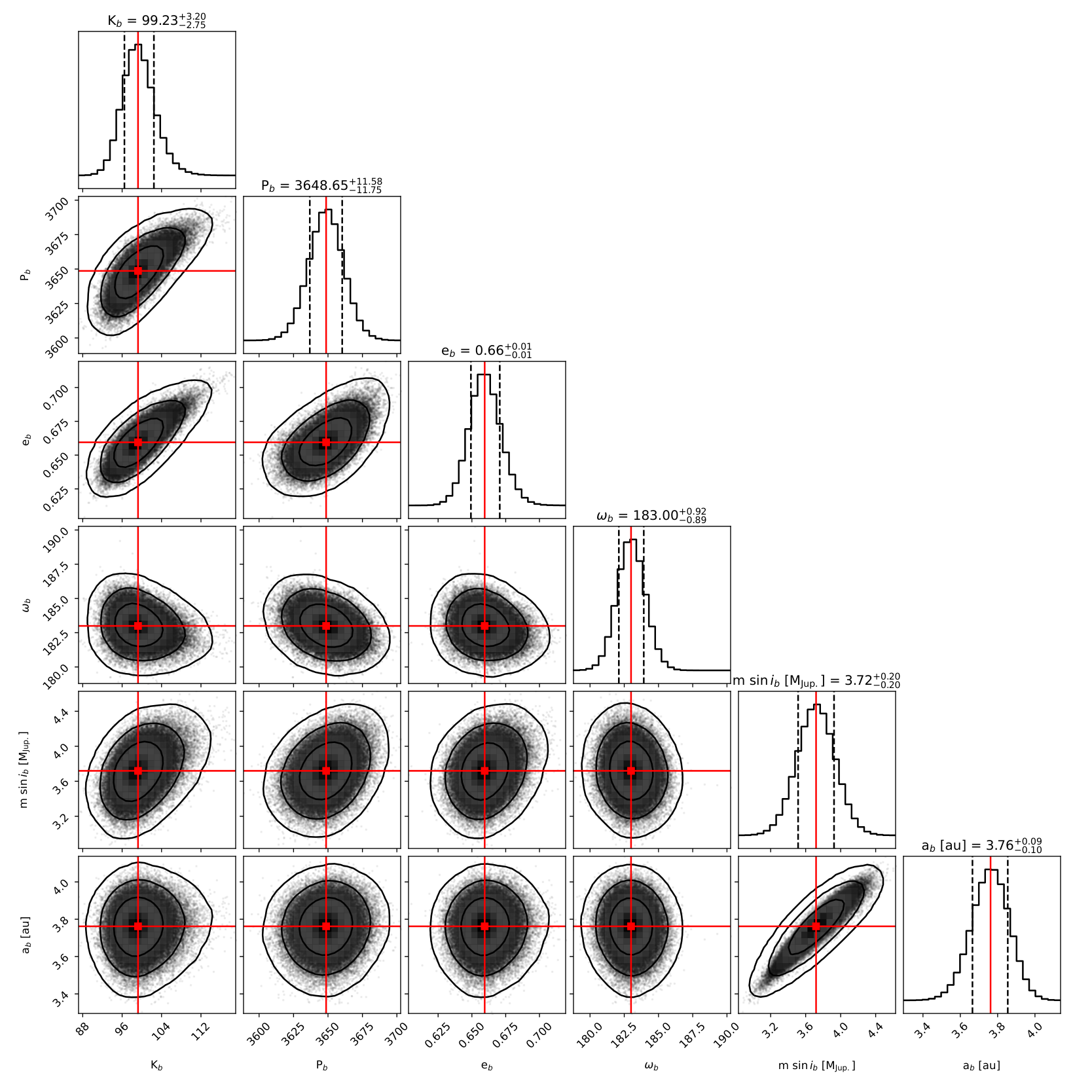
We recovered the RV signal with LICK, KECK, SONG, CARMENES and EXPRES using the Monte Carlo-Markov Chain (MCMC) method implemented in the Exo-Striker package (Trifonov 2019). We set 20 walkers and ran 1,000 burning phase steps and 10,000 MCMC phase steps in our analysis. We consider velocity offsets as the free parameters to fit simultaneously datasets originating from different spectrographs. We summarize the updated planetary parameters in Table 8. The orbital solution is plotted in Fig. 4 and the correlations between parameters together with the derived MCMC posterior probability distributions are presented in Fig. C.29 in the appendix.
In summary, we confirm the presence of a planet in this system. We agree with previous studies that the low levels of stellar activity (Wright et al. 2004) and photometric variability, along with the low scatter in RV measurements, make it very unlikely that the RV variations are caused by stellar activity. We did not find evidence of an additional companion in the system. Wittenmyer et al. 2013 proposed a 2-planet solution for HD3651, with the second planet in 2:1 resonance. We can rule out such a solution and confirm that the solution with a single eccentric planet also leads to the lowest fitted value. We also checked if the transit would be visible in the TESS data. Unfortunately, transits are just outside of the observing window in both sectors 17 and 57.


6.2 GJ 504
The GLS periodogram of the SONG data shows a significant peak at 3.67 days and another at 1.39 days (Fig. 5), which we assign to the rotation period and its 1-day alias. These two peaks also stand out in the periodograms of the HARPS-N and CARMENES datasets. In Section 5.2 we derive a rotation period of 3.4 days from the TESS LC.
The signal of the rotational period is not the most significant in SONG data. The highest peak is found at 300 days. We can see a similar peak even in the HARPS-N dataset despite the shorter timescale of observations. The short timescale makes the CARMENES dataset unsuitable for interpreting such a long signal; however, the observed trend looks to agree with the period of 300 days. To investigate this signal in more detail, we used the SONG H activity indicator together with the HARPS-N H activity indicator (Fig. 5). In the SONG H we see the signal at 300 days, and a similar peak can also be seen in the HARPS-N H, suggesting that this signal is most likely associated with stellar activity.
We plot the fit of the signal at 300 days for SONG, HARPS-N and CARMENES RVs in Fig. 6. Such a short activity cycle was previously observed for F-type stars (see Section 6.4); however, it was not observed for a G-type star.


6.3 HN Peg
The GLS periodogram of the SONG RVs shows the most significant peak at 5.1 days and another peak at 1.24 days (Fig. 7), which is a 1-day alias of the 5.1-day signal. The periodogram of RVs also shows a peak at 2.54 days and its 1-day alias at 1.64 days. The periodogram of the CARMENES data does not reveal any significant signal.
TESS did not observe this target yet; however, Messina & Guinan 2003 determined the rotation period of the star. They performed photometric observations with three different Automatic Photoelectric Telescopes at Fairborn Observatory in southern Arizona and inferred a variable stellar rotation between 4.59 and 5.17 days. Hence, we interpret the 5.10-day signal in RVs as a rotational period of the star and the 2.54-day signal to be the first harmonic of the rotation period.
We can see the peak at 5.1 days with its 1-day alias in the H activity indicator. This signal becomes more significant after removing a 420-day signal, which we interpret as systematic due to the window function. We confirm that the 5.1-day signal is linked with stellar activity. To conclude, we interpreted all signals to be linked to the stellar activity and did not find any evidence of a planetary companion.


6.4 HD 46588
The most dominant peak in the GLS periodogram of the SONG RVs is at 127 days (Fig. 9). In the CARMENES VIS RVs, we also detect a peak close to 127 days but poorly defined because of the short baseline. We find a strong correlation of 0.79 between the chromatic index (CRX) and the CARMENES RVs at 127 days, suggesting that this peak is associated with stellar activity. This interpretation is corroborated by the SONG H indicator of the SONG dataset. We interpret this signal as the magnetic cycle of the star. We plot the fit of this signal for the SONG and CARMENES RVs in Fig. 10.
In the SONG periodogram, we observe two other significant peaks at 224 days and 1 yr. The 1-yr peak is visible in the H indicator, representing the 1-year window function of the SONG dataset. However, this is not the case for the peak at 224 days; hence, there might be a chance it might have a Keplerian origin. We computed the statistical significance of the peak at days via the bootstrap randomisation process with realisations (Murdoch et al. 1993). We found a false-alarm probability lower than one per cent suggesting that it is unlikely that this peak is due to random noise. However, we cannot say whether this signal is due to a planetary companion or connected to the stellar magnetic cycle, as the SONG data does not always behave as the simple sinusoidal model predicts, making the magnetic activity more complex. Further monitoring is needed to understand this system better; however, we report this system to have a possible planetary candidate. Fitted planetary parameters are summarized in Table 8. The fit was performed on the RV residuals after removal of the activity cycle with a period of 127 days. The orbital solution is plotted in Fig. 11 and the correlations between parameters together with the derived MCMC posterior probability distributions are presented in Fig. C.30 in the appendix. We also performed a multidimensional GP approach (Rajpaul et al. 2015) to characterise the stellar and planetary signals in the SONG data using the PYANETI code (Barragán et al. 2022). We used the H indicator to constrain the stellar signal. We set wide priors for planet parameters based on the periodogram and the initial fit (see Figure 11). We found planetary parameters consistent in with the previous fit. Derived planetary parameters are summarized in Table 8. The plot of H and RV time series and inferred stellar and planetary models is shown in Figure C.28. We can see that the stellar+planetary model can describe the observed RVs quite well.
HD 46588 is extremely interesting in terms of stellar activity. The Sun has a 22-yr magnetic cycle. However, the physics underlying this phenomenon is still not well understood, similarly to activity cycles in other Sun-like stars. Long-term observations and monitoring of stars’ chromospheric activity can be used to study activity cycles and determine their periods (Wilson 1978; Baliunas et al. 1995; Hall et al. 2007; Isaacson & Fischer 2010; Hempelmann et al. 2016). Baliunas et al. 1995 measured activity cycles for more than 40 stars, with periods ranging between 2.5 and 20 years.

Baliunas et al. 1995 observed the star Boo (HD 120136), which first appears to have a typical chromospheric cycle of 11.60.5 years. Boo is an F7 spectral type star with an M2 type companion on a close orbit of 3.3 days. The rotation period is determined to be close to this value, indicating synchronization. However, what makes this star interesting is evidence of additional variability in the CaII line with a significantly shorter period than the original chromospheric cycle. Baliunas et al. 1997 determined a period of 116 days, later confirmed by Mengel et al. 2016 and Mittag et al. 2017 investigating the S-index with the NARVAL and TIGRE instruments, respectively. Mittag et al. 2017 also showed that the X-ray data support a periodicity of about 120 days, addressing an interesting question: if the fast activity period of Boo is representative of main-sequence F stars? Mittag et al. 2019 used analysis of S-index time series of F-type stars taken with the TIGRE telescope to discuss this question. They detect three more short-term cycles and one candidate between 0.5–1 year. They do not provide the number of investigated F-type stars, preventing us from discussing the statistics. However, Boo is still the star with the fastest magnetic cycle ever observed.


In this context, HD 46588 is a twin of Boo. The star has the same F7 spectral type and hosts an L9 type companion at the projected physical separation of 1420 au (Loutrel et al. 2011). We found evidence for a chromospheric cycle at 127 days. New discoveries indeed support that short-term activity cycles can be typical in F-type stars. Furthermore, we derived the age of HD 46588 about 2.5 Gyr, which indicates that such short-term activity cycles can cause strong RV variations also for relatively old stars. HD 118865 is the other F7 star in our sample. Our observations are only about 150 days for HD 118865, and we observe just a linear trend in RVs (Section 6.6). Further monitoring of F stars will bring more light to the discussion. However, the population of such stars with short-term activity cycles is starting to grow.
| HD 3651 | HD 46588 | HD 46588 (GP) | |
| () | |||
| (m/s) | |||
| (days) | |||
| (days) | |||
| (deg) | |||
| (days) | - | - | |
| (m/s) | - | - | |
| (days) | - | - | |
| - | - | ||
| (days) | - | - |
6.5 HD 203030
In the periodogram of the TESS LC, we observed two strong peaks at 6.5 and 13 days. Typically we would attribute peaks to be the rotation period with the first harmonic. However, visual investigation of the LC reveals strong variations at 6.5 days and the gap in the data so that the middle period is missing. Hence, the 13-day peak is an artefact of data sampling. We can confirm such a hypothesis with the vsini value derived from spectra. Assuming an inclination of 90 degrees, we can derive the upper limit for the rotation period, which is 7.2 days, close to 6.5 days but much lower than 13 days.

The GLS periodograms for the SONG RVs show a significant peak at 2.23 days, with its 1-day alias at 1.81 days. After fitting this signal with a simple sinusoidal, we observe a peak at 6.5 days, representing the stellar rotation. We found an RMS scatter due to activity to be about 35 m s-1, higher than the semi-amplitude of signals in the periodogram of HD 203030 and much higher than 5.87 m s-1 inferred for the quiet star HD 3651. Hence, we conclude that stellar activity plays a dominant role in RVs, and the 2.2-day signal is probably just the second harmonic of the rotation period. In the periodogram of CARMENES RVs, we do not see any significant peak. SONG H indicator reveals a signal at 7.14 days, while the CARMENES H and S-index indicators both reveal a signal at 6.62 days, confirming the star’s rotation period. We can also see a peak close to 2.23 days in S-index. All in all, we report that the variations in RVs are probably associated with stellar activity.

6.6 HD 118865
In the STELLA RVs, we observe a decreasing trend, which is not observed in the CARMENES dataset. It leads to a variety of possible solutions. In Fig. 15 we illustrate one solution at a period of 575 days. We observe a similar trend in the STELLA He activity indicator (He I line at 587.56 nm) (Fig. 14). Hence, we prefer the stellar activity scenario over the planetary companion even though the relatively large semi-amplitude and the fact that the star has an age of about 1 Gyr or older. The star has an F spectral type, and as we discussed above, the magnetic cycle with a period of hundreds of days would not be surprising even for relatively old stars. Further spectroscopic monitoring is needed to constrain the period of this signal.


7 Discussion
7.1 The role of wide companions on planet formation and evolution
Wide stellar companions can significantly affect the physical parameters of inner planets. Peculiarities in their parameter distributions were predicted (Mayer et al. 2005; Kraus et al. 2012; Kaib et al. 2013, e.g.,) and observed (Zucker & Mazeh 2002; Eggenberger et al. 2004; Fontanive & Bardalez Gagliuffi 2021, e.g.,). Eggenberger et al. 2004 compared orbital period, minimum planetary mass, and eccentricity for a sample of planets in systems with and without a wide stellar companion. They discussed two possible peculiarities identified in the distributions of short periodic planets. First, planets with periods below 40 days appear to have lower eccentricities when part of multi-stellar systems compared to planets around single stars. Second, the most massive short-periodic planets in their sample all belong to multi-stellar systems. However, at that time, only about a dozen multiple stellar systems with an exoplanet were known. Fontanive & Bardalez Gagliuffi 2021 performed an extensive search for visual co-moving binary companions to exoplanet-host stars using DR2 data in addition to known systems from literature. They compiled 938 stars, from which 186 are binaries, and 32 belong to hierarchical triples. They used all systems to study peculiarities in their parameter distributions similarly to Eggenberger et al. 2004. Specifically, they studied the mass and RV semi-amplitudes of planets, masses of primaries, and masses and separations of wide companions in these systems. To highlight some of their results, they found that (i) more massive planet-host stars are more often in multi-stellar systems, (ii) only close binaries ( 1000 au) seem to influence the formation or evolution of inner planets and (iii) the mass of the stellar companions has no significant effect on planetary properties.
We did not find any planets in our sample of stars with wide BD companions (only one planetary candidate in HD 46588), so we used a different approach to discuss possible peculiarities in parameter distributions. We downloaded the catalogues of systems of single planet-host stars and planet-host stars with wide stellar binaries from Fontanive & Bardalez Gagliuffi 2021 to produce similar plots as in Eggenberger et al. 2004 and Fontanive & Bardalez Gagliuffi 2021. We also consider the planet’s eccentricity distribution as it was not discussed in Fontanive & Bardalez Gagliuffi 2021. To these plots, we added for comparison the HD 3651 planet, HD 46588b planetary candidate and the four planets from systems with known wide BD companions from the literature (red points in Fig. 18) discussed in detail in Appendix C. We excluded HD 65216, HD 41004 and Indi, as these systems have different architectures. We also excluded GJ 229 because we are sceptic about the planetary nature of the reported signals.
To better understand our data, we may firstly compare the separations and masses of wide BD companions from the sample of the systems with known planets (discussed in Appendix C) and our sample of five systems (we put HD 3651 to the first group). Both samples are small; however, we did not notice any crucial differences. The first sample spans separations from 3 au up to 9000 au (3, 23, 476, 2500, 9000) while the second from 487 au to 9200 au (487, 784, 1420, 9200). With the current mass uncertainties, both samples practically span companion masses through the whole range typical for BDs.
The plot of the minimum planetary mass versus the orbital period of planets can be seen in Fig. 18. We also divided systems of single planet-host stars into two categories: Group 1 contains systems with one planet orbiting a star (black points in Fig. 18), and Group 2 is made of systems with multiple planets orbiting a star (grey points)44 4 We need to note, that such division reflects our current information about these systems. For example, systems from Group 1 can be, in fact, members of Group 2 with an undetected additional companion(s).. Similarly, we divided multi-stellar systems into two categories: Group 3 contains systems with one planet and a stellar companion orbiting a primary star (blue points in Fig. 18), and Group 4 is made of systems with a stellar companion and multiple planets (green points). The final sample consists of 504 systems in Group 1, 479 systems in Group 2, 173 systems in Group 3, and 103 systems in Group 4.


We do not see many planets more massive than from Group 2 and Group 4 at close orbital periods. Multi-planetary systems with a planet’s orbital periods below days mostly host less massive planets. The inward migration of more massive planets would disrupt the orbits of inner planets, which would lead to collisions or their ejection (Mustill et al. 2015; Saffe et al. 2017). We can also see that the upper end of the minimum planetary mass actually represents the population of BDs. While this paper focuses on the wide BD companions, here, we can also see BDs in closer orbits. Most of the systems in this mass region are from Group 1 and Group 3; hence, no additional planets are detected, suggesting that close BDs might prevent their existence. However, one would need to check how many of these systems were spectroscopically followed up with sufficient precision to detect planets. We also observe that the most distant companions in the plot are BDs, which is not so surprising because they are brighter than planets, hence, easier to detect by direct imaging.
As the majority of planets in systems with wide BDs lies in the mass region of Jovian planets between (Mordasini 2018; Spiegel et al. 2011), we took only planets from this region to create kernel density estimates (KDEs) of the distributions of planet period. We chose a Gaussian kernel and used the cross-validation approach to derive the KDE bandwidths providing good insights into potential underlying trends. The only planetary system with a wide BD that does not lie in this mass region is GJ 229, and we reported the RV signal in GJ 229 as a planetary candidate rather than a confirmed planet (Appendix C). We created the KDEs for three groups: planets in systems with a one star (Group 1 + Group 2), planets in systems with multiple stars (Group 3 + Group 4), and planets in systems with known wide BD companions. The distributions of the planetary period can be seen in Fig. 16. We observe the bimodal distribution of giant planets in the first two groups, which have two maxima around 5 days and 1000 days. However, both maxima are slightly shifted, and we observe an enhancement of short periodic planets in systems with a wide stellar companion. Giant planets are thought to form via core accretion in a proto-planetary disk at larger distances from stars than are often observed. Subsequent inward migration thus plays an important role in the existence of planets across a large variety of observed orbital periods (Lin et al. 1996; Bodenheimer et al. 2001, e.g.). Hence, enhanced migration seems to work for a large number of short-period planets. We do not observe such bimodal behaviour in the distribution of planets in the systems with a wide BD, as no short periodic planet with an orbital period below ten days is known so far. Our survey is sensitive to such planets, so we should have easily detected them (Section 7.2). To investigate the significance of these results, we performed two-sided Kolmogorov-Smirnov tests comparing each sub-population of planets using the python package Scipy, specifically the scipy.stats.ks_2samp55 5 https://docs.scipy.org/doc/scipy/reference/generated/scipy.stats.ks_2samp.html function. In other words, we tested the null hypothesis that the samples are drawn from the same distribution and used a p-value to support or reject this hypothesis. Comparing the distribution of planets around single stars with planets around stars with a stellar companion, we obtained the p-value of 0.029. However, comparing the group of planets around stars with a wide BD with planets around single stars, we obtained a p-value of 0.59, and with planets around stars with a stellar companion, we obtained a p-value of 0.41. Hence, we cannot confirm that the group of planets around stars with a wide BD follows its own distribution.
The distribution of minimum planetary mass can be seen in Fig. 17. Here we used all planets and divided them into the same three groups. Except for the population of planets around stars with a wide BD, we observe the bimodal distributions with two maxima around and . Using the two-sided Kolmogorov-Smirnov test, we obtained the p-value of 0.08 comparing the planets around stars with a BD companion to planets around single stars and the p-value of 0.34 comparing the planets around stars with a BD companion to planets around stars with a stellar companion. It can suggest that a wide BD influences the mass distribution of planets in a similar way as a wide stellar companion, and these planets follow a similar distribution. Or there may be even a gap against low-mass planets in systems with a wide BD. However, these results can be affected by several factors. As BDs cool in time and become less luminous, their detection is easier when the system is young. The stellar activity of such young stars then influences the detection limits of RV campaigns and can cause bias in the non-detection of low-massive planets. In Section 7.2 we show our detection limits, which are often not sufficient to detect such low-massive planets. These insufficient detection limits are also caused by typically relatively massive primary stars in systems with a wide BD. We also observe that sub-Jovian planets () are more often around single stars than around stars with a stellar companion, the trend already mentioned in Fontanive & Bardalez Gagliuffi 2021. The trend is probably caused by the fact that low-massive planets are easier to detect around low-mass M stars causing deeper transits and larger RV semi-amplitudes, and such stars have a lower rate of multiplicity in comparison to more massive stars (Salama et al. 2022).
The plot of the eccentricity versus the orbital period of planets can be seen in Fig. 19. Colours represent the previous division into four groups plus planets around stars with a wide BD companion (red). To compare different groups, we used the same approach as before, creating KDEs for each group (see Fig. 20). Group 1 has visually a slightly different distribution than Group 3 with an enhancement of small () and high () eccentricities. Comparing these two samples, we obtained a p-value of 0.012 from the two-sided Kolmogorov-Smirnov test, which means that these differences have a relatively high confidence level. Such enhancement of low eccentric planets is not surprising if we link it with the enhancement of short-period planets in systems with a wide stellar companion discussed above. We also compared Group 1 with Group 2 and found a p-value of 0.0008, which mean that planets in multi-planetary systems have a different distribution than single planets. We can see that planets in multi-planetary systems have lower eccentricities, and we observe only a few planets with an eccentricity larger than 0.5. Comparing Group 2 with Group 4, we obtained a p-value of 0.28; hence, we cannot rule out that these groups follow the same distribution.
As the planets in systems with wide BDs have periods larger than 50 days, we took only planets from this region to create kernel density estimates (KDEs) of the distributions of planet eccentricity (Fig. 21). We obtained the p-value of 0.0007 comparing this population to the Group 1 (black line in Fig. 21), 0.00002 comparing to the Group 2 (grey line), 0.002 comparing to the Group 3 (blue line) and 0.0001 comparing to the Group 4 (green line). It means that these planets, with a high confidence level, follow their own distribution with a maximum at . All of these planets in Fig. 19 have periods larger than 40 days and eccentricities larger than 0.4. One planet that does not meet these criteria is GJ 229 b. We reported in Appendix C the RV signal in GJ 229 as a planetary candidate rather than a confirmed planet. So far, systems with wide BD companions do not follow the trend of the decreasing number of systems toward higher eccentricities observed for the other groups. It can suggest that wide BDs significantly affect planetary systems or that the formation mechanisms differ.


7.2 Frequency of planets in our sample
We estimate individual detection limits before drawing any conclusions about the fraction of planets orbiting stars with wide BD companions. First, we used RV observations to measure the RMS scatter caused by stellar activity/error bars of observations for each star. Before the procedure, we subtracted signals observed in periodograms, which we linked to the activity to reduce the RMS scatter as much as possible (see Section 6). Specifically, we subtracted the best fit sinusoidal function with the given period. Each star shows a different level of activity, mainly due to age differences, from the less active star HD 3651 with RMS of 6 m/s consistent with error bars of SONG data, GJ 504 with RMS of 19 m/s, up to HD 118865 with RMS of 63.5 m/s from STELLA observations. Second, we simulated the data with the same cadence and baseline as our observations and added Gaussian noise with a sigma equal to the RMS scatter. These data simulate our observations taking into account their error bars and the activity level of each star. Then, we inserted a sinusoidal signal into these data (higher eccentricity with sufficient phase coverage would further improve our detection limits). On such prepared datasets, we used the Exo-Striker to perform the Keplerian fit of the inserted signal and ran MCMC analysis with 20 walkers, 1,000 burning phase steps, and 10,000 MCMC phase steps to compute the 3 error bars for the semi-amplitude of this signal, hence, 3 detection limits. We note that such detection limits would drop for specific periods based on the cadence or gaps in individual datasets; however, the cadences and timescales of our observations would enable us to detect most of the signals from several days up to several hundreds of days, so it is a reasonable simplification. Finally, we transformed the semi-amplitudes into minimum masses for all periods, as shown in Fig. 22. HD 3651 is the less active star, so the detection limit derived for the star is equal to the instrumental limit of the SONG spectrograph for a given number of observations. We see that the activity in other systems significantly affects our detection limits. The HD 118865 system observed with STELLA has lower RV precision than the targets observed with SONG. Based on our detection limits, we can often exclude more massive planets than Neptune for orbital periods of a few days and Saturn for orbital periods longer than hundreds of days, respectively. For quiet stars, we would be able to detect all planets from the literature.
Before driving any conclusion about the frequency of planets orbiting stars with wide BD companions, we need to decide whether to include the HD 3651 system in the statistical analysis. Our decision will greatly impact the results as it is the only system with a confirmed planet. One can argue that we should exclude HD 3651b because this planet was known prior to our project. However, our target selection process was based on the starting criteria that this system fulfils; hence, we would include it regardless of the presence of a known planet. However, the discovery of the wide BD companion (Mugrauer et al. 2006) was actually triggered by the known planet companion as authors studied the multiplicity of exoplanet host stars. It is making it no longer independent from the presence of the planet in the system. However, Luhman et al. 2007 later independently presented the discovery of the wide BD companion observing a large number of stars in the solar neighbourhood with the Spitzer Space Telescope. It suggests that the wide BD companion would probably be discovered regardless of the presence of a known planet; hence we decided to include HD 3651 in our statistical analysis. In any case, we provide the frequency of planets also for the case we do not include HD 3651.
Based on our sample of six systems, the frequency of planets orbiting stars with wide BD companions is between % (without the planetary candidate in the HD 46588 system included) and %66 6 The uncertainty of the frequency was estimated as (1) following Bonavita & Desidera 2007. (with the planetary candidate included). If we do not include HD 3651b, then the frequency of planets orbiting stars with wide BD companions is between 0 and %. The study by Bonavita & Desidera 2020 compares the frequency of giant planets around binaries and single stars, including different observable biases. The study did not reveal statistically significant difference with 5.1 ± 1.57 % occurrence rate for binaries and 6.3 ± 1.36 % occurrence rate for single stars. Given the small sample of studied systems, comparing the frequency of planets orbiting stars with wide BD companions to these frequencies has no informative value.
8 Summary
We characterise a sample of five systems with a wide BD companion and search for exoplanets with the radial velocity technique. One additional system with a known exoplanet, HD 3651, was used as a benchmark to test our detection capabilities, and we recovered the orbital solution and improved the precision of planet parameters.
We used spectroscopic observations and available photometry to derive a complete list of physical parameters for the systems in our sample, with a special focus on the age of the systems using complementary age techniques. We found our sample to be relatively young, with three systems in order of hundreds of millions of years, one with age close to one Gyr, and two with ages older than 2.5 Gyr. We used ages to improve the physical parameters of the wide companions considering several substellar evolutionary models. We confirm the BD nature of all companions and place GJ 504B in the planetary regime with a mass below the deuterium-burning limit.
In our sample of five stars, only one planetary candidate was identified in the HD 46588 system, while the other signals are attributed to stellar activity. Our lower sensitivity limit is for Neptune-mass planets at short periods of a few days and Saturn-mass planets at longer periods of hundreds of days. For less active systems such as HD 3651, we are sensitive to Neptune-mass planets at all periods up to 300 days, while for HD 118865, we are sensitive only to Jupiter-mass planets at all periods. With one planetary candidate and one confirmed planet in six observed systems, we derive a frequency of planets orbiting stars with wide BD companions of below 70% with the uncertainties included.
We summarised the properties of known planets orbiting five stars with wide BD companions. We considered planets in these systems together with the full sample of planet host stars with and without wide stellar companions to identify potential peculiarities in their parameter distributions. We detected the enhancement of planets with short periods below six days in systems with wide companions. We interpret it as a consequence of enhanced migration inwards closer to the host star. We also observe a break at the eccentricity of 0.5 with a small number of planets with higher eccentricities in multi-planetary systems. Finally, planets in systems with wide BD companions follow their own eccentricity distribution with a maximum at and have periods larger than 40 days, masses larger than , and eccentricities larger than 0.4.
Acknowledgements.
JS and PK would like to acknowledge support from MSMT grant LTT-20015. JS and PK acknowledge a travel budget from ERASMUS+ grant 2020-1-CZ01-KA203-078200. JS would like to acknowledge support from the Grant Agency of Charles University: GAUK No. 314421. NL was financially supported by the Ministerio de Economia y Competitividad and the Fondo Europeo de Desarrollo Regional (FEDER) under AYA2015-69350-C3-2-P. We thank warmly Matthias Zechmeister for running the SERVAL pipeline and sending us the CARMENES radial velocities.This research has made use of the Simbad and Vizier databases, operated at the centre de Données Astronomiques de Strasbourg (CDS), and of NASA’s Astrophysics Data System Bibliographic Services (ADS).
This work has made use of data from the European Space Agency (ESA) mission Gaia (https://www.cosmos.esa.int/gaia), processed by the Gaia Data Processing and Analysis Consortium (DPAC, https://www.cosmos.esa.int/web/gaia/dpac/consortium). Funding for the DPAC has been provided by national institutions, in particular the institutions participating in the Gaia Multilateral Agreement. We acknowledge the use of public TESS data from pipelines at the TESS Science Office and at the TESS Science Processing Operations Center. Resources supporting this work were provided by the NASA High-End Computing (HEC) Program through the NASA Advanced Supercomputing (NAS) Division at Ames Research Center for the production of the SPOC data products. This paper includes data collected with the TESS mission, obtained from the MAST data archive at the Space Telescope Science Institute (STScI). Funding for the TESS mission is provided by the NASA Explorer Program. STScI is operated by the Association of Universities for Research in Astronomy, Inc., under NASA contract NAS 5–26555. This publication makes use of VOSA, developed under the Spanish Virtual Observatory project supported by the Spanish MINECO through grant AyA2017-84089. VOSA has been partially updated by using funding from the European Union’s Horizon 2020 Research and Innovation Programme, under Grant Agreement nº 776403 (EXOPLANETS-A). The SONG data were obtained over several semesters through programme numbers P02-10, P03-08, P04-02, and P05-02 (PI Lodieu). The Danish SONG telescope in Tenerife, the Hertzsprung SONG telescope, is owned and operated by Aarhus University and the University of Copenhagen in collaboration with the Astrophysics Institute of the Canary Islands (IAC). It is financed by the Villum Kann Rasmussen Foundation, Carlsberg Foundation, the Danish Council for Independent Research — Natural Sciences (FNU), European Research Council, Danish National Research Foundation, Aarhus University, University of Copenhagen and Instituto de Astrofísica de Canarias.
Based on observations collected at the Centro Astronómico Hispano-Alemán (CAHA) at Calar Alto, operated jointly by Junta de Andalucía and Consejo Superior de Investigaciones Científicas (IAA-CSIC). The CARMENES dataset was obtained as part of programme number F19-3.5-011 (PI Lodieu). CARMENES is an instrument for the Centro Astronómico Hispano-Alemán de Calar Alto (CAHA, Almería, Spain). CARMENES is funded by the German Max-Planck-Gesellschaft (MPG), the Spanish Consejo Superior de Investigaciones Científicas (CSIC), the European Union through FEDER/ERF FICTS-2011-02 funds, and the members of the CARMENES Consortium (Max-Planck-Institut für Astronomie, Instituto de Astrofísica de Andalucía, Landessternwarte Königstuhl, Institut de Ciencies de l’Espai, Insitut für Astrophysik Göttingen, Universidad Complutense de Madrid, Thüringer Landessternwarte Tautenburg, Instituto de Astrofísica de Canarias, Hamburger Sternwarte, Centro de Astrobiología and Centro Astronómico Hispano-Alemán), with additional contri-butions by the Spanish Ministry of Economy, the German Science Foundation through the Major Research Instrumentation Programme and DFG Research Unit FOR2544 ”Blue Planets around Red Stars”, the Klaus Tschira Stiftung, the states of Baden-Württemberg and Niedersachsen, and by the Junta de Andalucía.
Based on observations made with the Italian Telescopio Nazionale Galileo (TNG) operated on the island of La Palma by the Fundación Galileo Galilei of the INAF (Istituto Nazionale di Astrofisica) at the Spanish Observatorio del Roque de los Muchachos of the Instituto de Astrofísica de Canarias. Part of the HARPS-N data used in this work have been downloaded from the TNG archive. Based on observations collected at the European Organisation for Astronomical Research in the Southern Hemisphere under ESO programmes 072.C-0488, 183.C-0972, 085.C-0019, 087.C-0831, 183.C-0972, 089.C-0732, 090.C-0421, 091.C-0034, 093.C-0409, 095.C-0551, 096.C-0460, 196.C-1006, 098.C-0366, 099.C-0458, 0100.C-0097, 0101.C-0379, 0102.C-0558, 0103.C-0432.
References
- Abbott et al. (2018) Abbott, T. M. C., Abdalla, F. B., Allam, S., et al. 2018, ApJS, 239, 18
- Abt (2009) Abt, H. A. 2009, ApJS, 180, 117
- Allard et al. (2012) Allard, F., Homeier, D., & Freytag, B. 2012, Philosophical Transactions of the Royal Society of London Series A, 370, 2765
- Aller et al. (2020) Aller, A., Lillo-Box, J., Jones, D., Miranda, L. F., & Barceló Forteza, S. 2020, A&A, 635, A128
- Anderson et al. (2010) Anderson, R. I., Reiners, A., & Solanki, S. K. 2010, A&A, 522, A81
- Angus et al. (2019) Angus, R., Morton, T. D., Foreman-Mackey, D., et al. 2019, AJ, 158, 173
- Antoci et al. (2013) Antoci, V., Handler, G., Grundahl, F., et al. 2013, MNRAS, 435, 1563
- Asplund et al. (2009) Asplund, M., Grevesse, N., Sauval, A. J., & Scott, P. 2009, ARA&A, 47, 481
- Auvergne et al. (2009) Auvergne, M., Bodin, P., Boisnard, L., et al. 2009, A&A, 506, 411
- Baliunas et al. (1995) Baliunas, S. L., Donahue, R. A., Soon, W. H., et al. 1995, ApJ, 438, 269
- Baliunas et al. (1997) Baliunas, S. L., Henry, G. W., Donahue, R. A., Fekel, F. C., & Soon, W. H. 1997, ApJ, 474, L119
- Baraffe et al. (2003) Baraffe, I., Chabrier, G., Barman, T. S., Allard, F., & Hauschildt, P. H. 2003, A&A, 402, 701
- Barber et al. (2006) Barber, R. J., Tennyson, J., Harris, G. J., & Tolchenov, R. N. 2006, MNRAS, 368, 1087
- Barragán et al. (2022) Barragán, O., Aigrain, S., Rajpaul, V. M., & Zicher, N. 2022, MNRAS, 509, 866
- Bayo et al. (2008) Bayo, A., Rodrigo, C., Barrado Y Navascués, D., et al. 2008, A&A, 492, 277
- Bensby et al. (2003) Bensby, T., Feltzing, S., & Lundström, I. 2003, A&A, 410, 527
- Blanco-Cuaresma (2019) Blanco-Cuaresma, S. 2019, MNRAS, 486, 2075
- Blanco-Cuaresma et al. (2014) Blanco-Cuaresma, S., Soubiran, C., Heiter, U., & Jofré, P. 2014, A&A, 569, A111
- Bodenheimer et al. (2001) Bodenheimer, P., Lin, D. N. C., & Mardling, R. A. 2001, ApJ, 548, 466
- Boisse et al. (2009) Boisse, I., Moutou, C., Vidal-Madjar, A., et al. 2009, A&A, 495, 959
- Bonavita & Desidera (2007) Bonavita, M. & Desidera, S. 2007, A&A, 468, 721
- Bonavita & Desidera (2020) Bonavita, M. & Desidera, S. 2020, Galaxies, 8, 16
- Bonnefoy et al. (2018) Bonnefoy, M., Perraut, K., Lagrange, A. M., et al. 2018, A&A, 618, A63
- Borucki et al. (2010) Borucki, W. J., Koch, D., Basri, G., et al. 2010, Science, 327, 977
- Boss (2006) Boss, A. P. 2006, ApJ, 641, 1148
- Bouchy & Sophie Team (2006) Bouchy, F. & Sophie Team. 2006, in Tenth Anniversary of 51 Peg-b: Status of and prospects for hot Jupiter studies, ed. L. Arnold, F. Bouchy, & C. Moutou, 319–325
- Brandt et al. (2020) Brandt, T. D., Dupuy, T. J., Bowler, B. P., et al. 2020, AJ, 160, 196
- Bressan et al. (2012) Bressan, A., Marigo, P., Girardi, L., et al. 2012, MNRAS, 427, 127
- Brewer et al. (2020) Brewer, J. M., Fischer, D. A., Blackman, R. T., et al. 2020, AJ, 160, 67
- Burgasser (2007) Burgasser, A. J. 2007, ApJ, 658, 617
- Burgasser (2014) Burgasser, A. J. 2014, in Astronomical Society of India Conference Series, Vol. 11, Astronomical Society of India Conference Series, 7–16
- Burgasser & Splat Development Team (2017) Burgasser, A. J. & Splat Development Team. 2017, in Astronomical Society of India Conference Series, Vol. 14, Astronomical Society of India Conference Series, 7–12
- Burningham et al. (2013) Burningham, B., Cardoso, C. V., Smith, L., et al. 2013, MNRAS, 433, 457
- Burrows et al. (2001) Burrows, A., Hubbard, W. B., Lunine, J. I., & Liebert, J. 2001, Reviews of Modern Physics, 73, 719
- Butler et al. (1997) Butler, R. P., Marcy, G. W., Williams, E., Hauser, H., & Shirts, P. 1997, ApJ, 474, L115
- Butler et al. (2017) Butler, R. P., Vogt, S. S., Laughlin, G., et al. 2017, AJ, 153, 208
- Caballero et al. (2016) Caballero, J. A., Guàrdia, J., López del Fresno, M., et al. 2016, in Society of Photo-Optical Instrumentation Engineers (SPIE) Conference Series, Vol. 9910, Observatory Operations: Strategies, Processes, and Systems VI, ed. A. B. Peck, R. L. Seaman, & C. R. Benn, 99100E
- Caffau et al. (2011) Caffau, E., Ludwig, H. G., Steffen, M., Freytag, B., & Bonifacio, P. 2011, Sol. Phys., 268, 255
- Carmichael et al. (2020) Carmichael, T. W., Quinn, S. N., Mustill, A. J., et al. 2020, AJ, 160, 53
- Carmichael et al. (2021) Carmichael, T. W., Quinn, S. N., Zhou, G., et al. 2021, AJ, 161, 97
- Carnero Rosell et al. (2019) Carnero Rosell, A., Santiago, B., dal Ponte, M., et al. 2019, MNRAS, 489, 5301
- Cayrel et al. (2011) Cayrel, R., van’t Veer-Menneret, C., Allard, N. F., & Stehlé, C. 2011, A&A, 531, A83
- Chambers et al. (2016) Chambers, K. C., Magnier, E. A., Metcalfe, N., et al. 2016, arXiv e-prints, arXiv:1612.05560
- Cheetham et al. (2018) Cheetham, A., Ségransan, D., Peretti, S., et al. 2018, A&A, 614, A16
- Choi et al. (2016) Choi, J., Dotter, A., Conroy, C., et al. 2016, ApJ, 823, 102
- Cincunegui et al. (2007) Cincunegui, C., Díaz, R. F., & Mauas, P. J. D. 2007, A&A, 469, 309
- Coelho (2014) Coelho, P. R. T. 2014, MNRAS, 440, 1027
- Cosentino et al. (2012) Cosentino, R., Lovis, C., Pepe, F., et al. 2012, in Society of Photo-Optical Instrumentation Engineers (SPIE) Conference Series, Vol. 8446, Ground-based and Airborne Instrumentation for Astronomy IV, ed. I. S. McLean, S. K. Ramsay, & H. Takami, 84461V
- Cruz et al. (2007) Cruz, K. L., Reid, I. N., Kirkpatrick, J. D., et al. 2007, AJ, 133, 439
- Curtis et al. (2020) Curtis, J. L., Agüeros, M. A., Matt, S. P., et al. 2020, ApJ, 904, 140
- Cutri et al. (2003) Cutri, R. M., Skrutskie, M. F., van Dyk, S., et al. 2003, VizieR Online Data Catalog, II/246
- Cutri et al. (2021) Cutri, R. M., Wright, E. L., Conrow, T., et al. 2021, VizieR Online Data Catalog, II/328
- da Silva et al. (2006) da Silva, L., Girardi, L., Pasquini, L., et al. 2006, A&A, 458, 609
- dal Ponte et al. (2020) dal Ponte, M., Santiago, B., Carnero Rosell, A., et al. 2020, MNRAS, 499, 5302
- Deacon et al. (2014) Deacon, N. R., Liu, M. C., Magnier, E. A., et al. 2014, ApJ, 792, 119
- Deacon et al. (2012) Deacon, N. R., Liu, M. C., Magnier, E. A., et al. 2012, ApJ, 755, 94
- Deming et al. (2015) Deming, D., Knutson, H., Kammer, J., et al. 2015, ApJ, 805, 132
- Desidera & Barbieri (2007) Desidera, S. & Barbieri, M. 2007, A&A, 462, 345
- Dieterich et al. (2018) Dieterich, S. B., Weinberger, A. J., Boss, A. P., et al. 2018, ApJ, 865, 28
- Donahue et al. (1996) Donahue, R. A., Saar, S. H., & Baliunas, S. L. 1996, ApJ, 466, 384
- D’Orazi et al. (2017) D’Orazi, V., Desidera, S., Gratton, R. G., et al. 2017, A&A, 598, A19
- Ednie et al. (2018) Ednie, M., Follette, K., & Ward-Duong, K. 2018, in American Astronomical Society Meeting Abstracts, Vol. 231, American Astronomical Society Meeting Abstracts #231, 349.15
- Eggenberger et al. (2004) Eggenberger, A., Udry, S., & Mayor, M. 2004, A&A, 417, 353
- Endl et al. (2002) Endl, M., Kürster, M., Els, S., et al. 2002, A&A, 392, 671
- Epchtein et al. (1997) Epchtein, N., de Batz, B., Capoani, L., et al. 1997, The Messenger, 87, 27
- Feng et al. (2019) Feng, F., Anglada-Escudé, G., Tuomi, M., et al. 2019, MNRAS, 490, 5002
- Feng et al. (2020) Feng, F., Butler, R. P., Shectman, S. A., et al. 2020, ApJS, 246, 11
- Fischer et al. (2003) Fischer, D. A., Butler, R. P., Marcy, G. W., Vogt, S. S., & Henry, G. W. 2003, ApJ, 590, 1081
- Fischer et al. (2014) Fischer, D. A., Marcy, G. W., & Spronck, J. F. P. 2014, ApJS, 210, 5
- Fontanive & Bardalez Gagliuffi (2021) Fontanive, C. & Bardalez Gagliuffi, D. 2021, Frontiers in Astronomy and Space Sciences, 8, 16
- Frasca et al. (2018) Frasca, A., Guillout, P., Klutsch, A., et al. 2018, A&A, 612, A96
- Fredslund Andersen et al. (2019) Fredslund Andersen, M., Handberg, R., Weiss, E., et al. 2019, PASP, 131, 045003
- Fridlund et al. (2017) Fridlund, M., Gaidos, E., Barragán, O., et al. 2017, A&A, 604, A16
- Fuhrmann & Chini (2015) Fuhrmann, K. & Chini, R. 2015, ApJ, 806, 163
- Gagné et al. (2018) Gagné, J., Mamajek, E. E., Malo, L., et al. 2018, ApJ, 856, 23
- Gaia Collaboration et al. (2018a) Gaia Collaboration, Babusiaux, C., van Leeuwen, F., et al. 2018a, A&A, 616, A10
- Gaia Collaboration et al. (2018b) Gaia Collaboration, Brown, A. G. A., Vallenari, A., et al. 2018b, A&A, 616, A1
- Gaia Collaboration et al. (2021) Gaia Collaboration, Brown, A. G. A., Vallenari, A., et al. 2021, A&A, 649, A1
- Gaidos (1998) Gaidos, E. J. 1998, PASP, 110, 1259
- Geißler et al. (2008) Geißler, K., Chauvin, G., & Sterzik, M. F. 2008, A&A, 480, 193
- Ghezzi et al. (2010) Ghezzi, L., Cunha, K., Smith, V. V., et al. 2010, ApJ, 720, 1290
- Godoy-Rivera et al. (2021) Godoy-Rivera, D., Pinsonneault, M. H., & Rebull, L. M. 2021, ApJS, 257, 46
- Gray et al. (2001) Gray, R. O., Napier, M. G., & Winkler, L. I. 2001, AJ, 121, 2148
- Green (2018) Green, G. M. 2018, The Journal of Open Source Software, 3, 695
- Green et al. (2019) Green, G. M., Schlafly, E., Zucker, C., Speagle, J. S., & Finkbeiner, D. 2019, ApJ, 887, 93
- Grevesse et al. (1993) Grevesse, N., Noels, A., & Sauval, A. J. 1993, A&A, 271, 587
- Grundahl et al. (2017) Grundahl, F., Fredslund Andersen, M., Christensen-Dalsgaard, J., et al. 2017, ApJ, 836, 142
- Gustafsson et al. (2008) Gustafsson, B., Edvardsson, B., Eriksson, K., et al. 2008, A&A, 486, 951
- Hall et al. (2007) Hall, J. C., Lockwood, G. W., & Skiff, B. A. 2007, AJ, 133, 862
- Heiter et al. (2015) Heiter, U., Lind, K., Asplund, M., et al. 2015, Phys. Scr, 90, 054010
- Hempelmann et al. (2016) Hempelmann, A., Mittag, M., Gonzalez-Perez, J. N., et al. 2016, A&A, 586, A14
- Hinkley et al. (2015) Hinkley, S., Kraus, A. L., Ireland, M. J., et al. 2015, ApJ, 806, L9
- Høg et al. (2000) Høg, E., Fabricius, C., Makarov, V. V., et al. 2000, A&A, 357, 367
- Houk & Swift (1999) Houk, N. & Swift, C. 1999, Michigan Spectral Survey, 5, 0
- Isaacson & Fischer (2010) Isaacson, H. & Fischer, D. 2010, ApJ, 725, 875
- Ishihara et al. (2010) Ishihara, D., Onaka, T., Kataza, H., et al. 2010, A&A, 514, A1
- Jackson et al. (2012) Jackson, A. P., Davis, T. A., & Wheatley, P. J. 2012, MNRAS, 422, 2024
- Janson et al. (2013) Janson, M., Brandt, T. D., Kuzuhara, M., et al. 2013, ApJ, 778, L4
- Jones et al. (1997) Jones, B. F., Fischer, D., Shetrone, M., & Soderblom, D. R. 1997, AJ, 114, 352
- Jones et al. (1999) Jones, B. F., Fischer, D., & Soderblom, D. R. 1999, AJ, 117, 330
- Jurgenson et al. (2016) Jurgenson, C., Fischer, D., McCracken, T., et al. 2016, in Society of Photo-Optical Instrumentation Engineers (SPIE) Conference Series, Vol. 9908, Ground-based and Airborne Instrumentation for Astronomy VI, ed. C. J. Evans, L. Simard, & H. Takami, 99086T
- Kaib et al. (2013) Kaib, N. A., Raymond, S. N., & Duncan, M. 2013, Nature, 493, 381
- Keenan & McNeil (1989) Keenan, P. C. & McNeil, R. C. 1989, ApJS, 71, 245
- Kirkpatrick et al. (2011) Kirkpatrick, J. D., Cushing, M. C., Gelino, C. R., et al. 2011, ApJS, 197, 19
- Korzennik et al. (2000) Korzennik, S. G., Brown, T. M., Fischer, D. A., Nisenson, P., & Noyes, R. W. 2000, ApJ, 533, L147
- Kraus et al. (2012) Kraus, A. L., Ireland, M. J., Hillenbrand, L. A., & Martinache, F. 2012, ApJ, 745, 19
- Kuzuhara et al. (2013) Kuzuhara, M., Tamura, M., Kudo, T., et al. 2013, ApJ, 774, 11
- Lawrence et al. (2007) Lawrence, A., Warren, S. J., Almaini, O., et al. 2007, MNRAS, 379, 1599
- Leggett (1992) Leggett, S. K. 1992, ApJS, 82, 351
- Lightkurve Collaboration et al. (2018) Lightkurve Collaboration, Cardoso, J. V. d. M., Hedges, C., et al. 2018, Lightkurve: Kepler and TESS time series analysis in Python, Astrophysics Source Code Library
- Lin et al. (1996) Lin, D. N. C., Bodenheimer, P., & Richardson, D. C. 1996, Nature, 380, 606
- Liu et al. (2010) Liu, M. C., Dupuy, T. J., & Leggett, S. K. 2010, ApJ, 722, 311
- Liu et al. (2007) Liu, M. C., Leggett, S. K., & Chiu, K. 2007, ApJ, 660, 1507
- Lodieu et al. (2012) Lodieu, N., Burningham, B., Day-Jones, A., et al. 2012, A&A, 548, A53
- Lodieu et al. (2014) Lodieu, N., Pérez-Garrido, A., Béjar, V. J. S., et al. 2014, A&A, 569, A120
- Lodieu et al. (2007) Lodieu, N., Pinfield, D. J., Leggett, S. K., et al. 2007, MNRAS, 379, 1423
- Loutrel et al. (2011) Loutrel, N. P., Luhman, K. L., Lowrance, P. J., & Bochanski, J. J. 2011, ApJ, 739, 81
- Luhman et al. (2007) Luhman, K. L., Patten, B. M., Marengo, M., et al. 2007, ApJ, 654, 570
- Marcy et al. (2001) Marcy, G. W., Butler, R. P., Vogt, S. S., et al. 2001, ApJ, 555, 418
- Martín et al. (1999) Martín, E. L., Delfosse, X., Basri, G., et al. 1999, AJ, 118, 2466
- Mayer et al. (2005) Mayer, L., Wadsley, J., Quinn, T., & Stadel, J. 2005, MNRAS, 363, 641
- Mayor et al. (2004) Mayor, M., Udry, S., Naef, D., et al. 2004, A&A, 415, 391
- McCaughrean et al. (2004) McCaughrean, M. J., Close, L. M., Scholz, R. D., et al. 2004, A&A, 413, 1029
- McMahon et al. (2013) McMahon, R. G., Banerji, M., Gonzalez, E., et al. 2013, The Messenger, 154, 35
- Mengel et al. (2016) Mengel, M. W., Fares, R., Marsden, S. C., et al. 2016, MNRAS, 459, 4325
- Mentuch et al. (2008) Mentuch, E., Brandeker, A., van Kerkwijk, M. H., Jayawardhana, R., & Hauschildt, P. H. 2008, ApJ, 689, 1127
- Messina & Guinan (2003) Messina, S. & Guinan, E. F. 2003, A&A, 409, 1017
- Metchev & Hillenbrand (2006) Metchev, S. A. & Hillenbrand, L. A. 2006, ApJ, 651, 1166
- Miles-Páez et al. (2017) Miles-Páez, P. A., Metchev, S., Luhman, K. L., Marengo, M., & Hulsebus, A. 2017, AJ, 154, 262
- Mittag et al. (2017) Mittag, M., Robrade, J., Schmitt, J. H. M. M., et al. 2017, A&A, 600, A119
- Mittag et al. (2019) Mittag, M., Schmitt, J. H. M. M., Hempelmann, A., & Schröder, K. P. 2019, A&A, 621, A136
- Mordasini (2018) Mordasini, C. 2018, in Handbook of Exoplanets, ed. H. J. Deeg & J. A. Belmonte, 143
- Moriwaki & Nakagawa (2004) Moriwaki, K. & Nakagawa, Y. 2004, ApJ, 609, 1065
- Mugrauer et al. (2004) Mugrauer, M., Neuhäuser, R., Mazeh, T., Guenther, E., & Fernández, M. 2004, Astronomische Nachrichten, 325, 718
- Mugrauer et al. (2005) Mugrauer, M., Neuhäuser, R., Seifahrt, A., Mazeh, T., & Guenther, E. 2005, A&A, 440, 1051
- Mugrauer et al. (2007) Mugrauer, M., Seifahrt, A., & Neuhäuser, R. 2007, MNRAS, 378, 1328
- Mugrauer et al. (2006) Mugrauer, M., Seifahrt, A., Neuhäuser, R., & Mazeh, T. 2006, MNRAS, 373, L31
- Murdoch et al. (1993) Murdoch, K. A., Hearnshaw, J. B., & Clark, M. 1993, ApJ, 413, 349
- Mustill et al. (2015) Mustill, A. J., Davies, M. B., & Johansen, A. 2015, ApJ, 808, 14
- Nakajima et al. (1995) Nakajima, T., Oppenheimer, B. R., Kulkarni, S. R., et al. 1995, Nature, 378, 463
- Nelson (2003) Nelson, R. P. 2003, MNRAS, 345, 233
- Palle et al. (2021) Palle, E., Luque, R., Zapatero Osorio, M. R., et al. 2021, A&A, 650, A55
- Paunzen (2015) Paunzen, E. 2015, A&A, 580, A23
- Pecaut & Mamajek (2013) Pecaut, M. J. & Mamajek, E. E. 2013, ApJS, 208, 9
- Persson et al. (2019) Persson, C. M., Csizmadia, S., Mustill, A. J., et al. 2019, A&A, 628, A64
- Pilyavsky et al. (2011) Pilyavsky, G., Mahadevan, S., Kane, S. R., et al. 2011, ApJ, 743, 162
- Piskunov & Valenti (2017) Piskunov, N. & Valenti, J. A. 2017, A&A, 597, A16
- Quirrenbach et al. (2014) Quirrenbach, A., Amado, P. J., Caballero, J. A., et al. 2014, in Society of Photo-Optical Instrumentation Engineers (SPIE) Conference Series, Vol. 9147, Ground-based and Airborne Instrumentation for Astronomy V, ed. S. K. Ramsay, I. S. McLean, & H. Takami, 91471F
- Quirrenbach et al. (2019) Quirrenbach, A., Trifonov, T., Lee, M. H., & Reffert, S. 2019, A&A, 624, A18
- Rajpaul et al. (2015) Rajpaul, V., Aigrain, S., Osborne, M. A., Reece, S., & Roberts, S. 2015, MNRAS, 452, 2269
- Ricker et al. (2015) Ricker, G. R., Winn, J. N., Vanderspek, R., et al. 2015, Journal of Astronomical Telescopes, Instruments, and Systems, 1, 014003
- Riedel et al. (2017) Riedel, A. R., Blunt, S. C., Lambrides, E. L., et al. 2017, AJ, 153, 95
- Rodrigues et al. (2017) Rodrigues, T. S., Bossini, D., Miglio, A., et al. 2017, MNRAS, 467, 1433
- Rodrigues et al. (2014) Rodrigues, T. S., Girardi, L., Miglio, A., et al. 2014, MNRAS, 445, 2758
- Rosenthal et al. (2021) Rosenthal, L. J., Fulton, B. J., Hirsch, L. A., et al. 2021, ApJS, 255, 8
- Saffe et al. (2017) Saffe, C., Jofré, E., Martioli, E., et al. 2017, A&A, 604, L4
- Salama et al. (2022) Salama, M., Ziegler, C., Baranec, C., et al. 2022, AJ, 163, 200
- Santos et al. (2002) Santos, N. C., Mayor, M., Naef, D., et al. 2002, A&A, 392, 215
- Saumon & Marley (2008) Saumon, D. & Marley, M. S. 2008, ApJ, 689, 1327
- Scholz et al. (2003) Scholz, R. D., McCaughrean, M. J., Lodieu, N., & Kuhlbrodt, B. 2003, A&A, 398, L29
- Ségransan et al. (2011) Ségransan, D., Mayor, M., Udry, S., et al. 2011, A&A, 535, A54
- Skemer et al. (2016) Skemer, A. J., Morley, C. V., Zimmerman, N. T., et al. 2016, ApJ, 817, 166
- Skrutskie et al. (2006) Skrutskie, M. F., Cutri, R. M., Stiening, R., et al. 2006, AJ, 131, 1163
- Soderblom et al. (1993a) Soderblom, D. R., Fedele, S. B., Jones, B. F., Stauffer, J. R., & Prosser, C. F. 1993a, AJ, 106, 1080
- Soderblom et al. (1993b) Soderblom, D. R., Jones, B. F., Balachandran, S., et al. 1993b, AJ, 106, 1059
- Soderblom et al. (1990) Soderblom, D. R., Oey, M. S., Johnson, D. R. H., & Stone, R. P. S. 1990, AJ, 99, 595
- Soderblom et al. (1993c) Soderblom, D. R., Pilachowski, C. A., Fedele, S. B., & Jones, B. F. 1993c, AJ, 105, 2299
- Spiegel et al. (2011) Spiegel, D. S., Burrows, A., & Milsom, J. A. 2011, ApJ, 727, 57
- Stassun et al. (2017) Stassun, K. G., Collins, K. A., & Gaudi, B. S. 2017, AJ, 153, 136
- Stassun et al. (2006) Stassun, K. G., Mathieu, R. D., & Valenti, J. A. 2006, Nature, 440, 311
- Stassun et al. (2019) Stassun, K. G., Oelkers, R. J., Paegert, M., et al. 2019, AJ, 158, 138
- Stassun et al. (2018) Stassun, K. G., Oelkers, R. J., Pepper, J., et al. 2018, AJ, 156, 102
- Strassmeier et al. (2004) Strassmeier, K. G., Granzer, T., Weber, M., et al. 2004, Astronomische Nachrichten, 325, 527
- Takeda et al. (2007) Takeda, G., Ford, E. B., Sills, A., et al. 2007, ApJS, 168, 297
- Tamuz et al. (2008) Tamuz, O., Ségransan, D., Udry, S., et al. 2008, A&A, 480, L33
- Triaud et al. (2020) Triaud, A. H. M. J., Burgasser, A. J., Burdanov, A., et al. 2020, Nature Astronomy, 4, 650
- Trifonov (2019) Trifonov, T. 2019, The Exo-Striker: Transit and radial velocity interactive fitting tool for orbital analysis and N-body simulations
- Trifonov et al. (2018) Trifonov, T., Kürster, M., Zechmeister, M., et al. 2018, A&A, 609, A117
- Tsantaki et al. (2014) Tsantaki, M., Sousa, S. G., Santos, N. C., et al. 2014, A&A, 570, A80
- Tsvetanov et al. (2000) Tsvetanov, Z. I., Golimowski, D. A., Zheng, W., et al. 2000, ApJ, 531, L61
- Tull (1998) Tull, R. G. 1998, in Society of Photo-Optical Instrumentation Engineers (SPIE) Conference Series, Vol. 3355, Optical Astronomical Instrumentation, ed. S. D’Odorico, 387–398
- Tull et al. (1995) Tull, R. G., MacQueen, P. J., Sneden, C., & Lambert, D. L. 1995, PASP, 107, 251
- Tuomi et al. (2014) Tuomi, M., Jones, H. R. A., Barnes, J. R., Anglada-Escudé, G., & Jenkins, J. S. 2014, MNRAS, 441, 1545
- Valenti & Piskunov (1996) Valenti, J. A. & Piskunov, N. 1996, A&AS, 118, 595
- Voges et al. (1999) Voges, W., Aschenbach, B., Boller, T., et al. 1999, A&A, 349, 389
- Vogt (1987) Vogt, S. S. 1987, PASP, 99, 1214
- Vogt et al. (1994) Vogt, S. S., Allen, S. L., Bigelow, B. C., et al. 1994, in Society of Photo-Optical Instrumentation Engineers (SPIE) Conference Series, Vol. 2198, Instrumentation in Astronomy VIII, ed. D. L. Crawford & E. R. Craine, 362
- Šubjak et al. (2020) Šubjak, J., Sharma, R., Carmichael, T. W., et al. 2020, AJ, 159, 151
- Weber et al. (2008) Weber, M., Granzer, T., Strassmeier, K. G., & Woche, M. 2008, in Society of Photo-Optical Instrumentation Engineers (SPIE) Conference Series, Vol. 7019, Advanced Software and Control for Astronomy II, ed. A. Bridger & N. M. Radziwill, 70190L
- Wilson et al. (2001) Wilson, J. C., Kirkpatrick, J. D., Gizis, J. E., et al. 2001, AJ, 122, 1989
- Wilson (1978) Wilson, O. C. 1978, ApJ, 226, 379
- Wittenmyer et al. (2019) Wittenmyer, R. A., Clark, J. T., Zhao, J., et al. 2019, MNRAS, 484, 5859
- Wittenmyer et al. (2009) Wittenmyer, R. A., Endl, M., Cochran, W. D., Levison, H. F., & Henry, G. W. 2009, ApJS, 182, 97
- Wittenmyer et al. (2013) Wittenmyer, R. A., Wang, S., Horner, J., et al. 2013, ApJS, 208, 2
- Wright et al. (2010) Wright, E. L., Eisenhardt, P. R. M., Mainzer, A. K., et al. 2010, AJ, 140, 1868
- Wright et al. (2004) Wright, J. T., Marcy, G. W., Butler, R. P., & Vogt, S. S. 2004, ApJS, 152, 261
- Wright et al. (2011) Wright, N. J., Drake, J. J., Mamajek, E. E., & Henry, G. W. 2011, ApJ, 743, 48
- York et al. (2000) York, D. G., Adelman, J., Anderson, John E., J., et al. 2000, AJ, 120, 1579
- Zechmeister & Kürster (2009) Zechmeister, M. & Kürster, M. 2009, A&A, 496, 577
- Zechmeister et al. (2018) Zechmeister, M., Reiners, A., Amado, P. J., et al. 2018, A&A, 609, A12
- Zucker & Mazeh (2002) Zucker, S. & Mazeh, T. 2002, ApJ, 568, L113
- Zucker et al. (2003) Zucker, S., Mazeh, T., Santos, N. C., Udry, S., & Mayor, M. 2003, A&A, 404, 775
- Zucker et al. (2004) Zucker, S., Mazeh, T., Santos, N. C., Udry, S., & Mayor, M. 2004, A&A, 426, 695
- Zuckerman (2019) Zuckerman, B. 2019, ApJ, 870, 27
Appendix A Stellar and brown dwarf parameters
A.1 Stellar parameters with iSpec
We used the iSpec framework (Blanco-Cuaresma et al. 2014; Blanco-Cuaresma 2019) to derive the parameters of the host stars. We used the Spectroscopy Made Easy radiative transfer code (Valenti & Piskunov 1996; Piskunov & Valenti 2017, SME;) incorporated into the iSpec framework, and complementary to it, we use the MARCS atmosphere models (Gustafsson et al. 2008), and version 5 of the GES atomic line list (Heiter et al. 2015). The spectral fitting technique minimizes the value between the calculated synthetic spectrum and the observed spectrum.
We used SERVAL to co-add all CARMENES spectra to the very high signal-to-noise final spectrum. We then used these final spectra for each system from our sample to determine the effective temperature , metallicity , surface gravity , the projected stellar equatorial velocity , and the lithium equivalent width of the Li I line at 670.8 nm following the same procedure as in Fridlund et al. 2017. In our analysis, we computed values for the micro-turbulence and macro-turbulence velocities (Vmic, Vmac) from empirical relations incorporated into the iSpec framework. To determine , we fit the wings of H Balmer line (Cayrel et al. 2011). We then used this temperature to fit the line wings of the Ca I triplet (610.27 nm) to derive a value of . We also used a large sample of clean and unblended Fe I lines in the interval from 597 nm to 643 nm to derive and . We report the stellar parameters for the stars of our sample in Table 5.
To estimate stellar mass and radius, we used the Bayesian parameter estimation code PARAM 1.577 7 http://stev.oapd.inaf.it/cgi-bin/param_1.3 (da Silva et al. 2006; Rodrigues et al. 2014; Rodrigues et al. 2017) based on the PARSEC isochrones. As input parameters, we set eDR3 parallaxes, DR2 magnitudes, luminosities from VOSA, and with derived from iSpec. We report all derived parameters in Table 5.
A.2 SED analysis with VOSA
As an independent check, we used the Virtual Observatory SED Analyser (Bayo et al. 2008, VOSA88 8 http://svo2.cab.inta-csic.es/theory/vosa/;) to determine stellar parameters. To model the spectral energy distribution of the stars in our sample we used grids of five different models: BT-Settl-AGSS2009 (Barber et al. 2006; Asplund et al. 2009; Allard et al. 2012), BT-Settl-CIFIST (Barber et al. 2006; Caffau et al. 2011; Allard et al. 2012), BT-NextGen GNS93 (Grevesse et al. 1993; Barber et al. 2006; Allard et al. 2012), BT-NextGen AGSS2009 (Barber et al. 2006; Asplund et al. 2009; Allard et al. 2012), and Coelho Synthetic stellar library (Coelho 2014) and performed the minimization procedure to compare theoretical models with the observed photometry. We used the available photometric measurements, specifically, the Strömgren-Crawford uvby (Paunzen 2015), Tycho (Høg et al. 2000), DR2 (Gaia Collaboration et al. 2018b), eDR3 (Gaia Collaboration et al. 2021), 2MASS (Cutri et al. 2003), AKARI (Ishihara et al. 2010), and WISE (Cutri et al. 2021) photometry. We set priors for the Teff = 4000–7000 K, (g) = 4.0–5.0 dex, and [Fe/H] = 0.5–0.5 based on results from iSpec. For each model, we take only results with the lowest , and use them to create the final intervals of derived parameters. We report the final intervals in Table 5. In Table 5, we also compare the stellar radii computed from stellar isochrones with ones from VOSA determined via the Stefan–Boltzmann law.
A.3 Revised parameters of the wide BD companions
We used the SpeX Prism Library Analysis Toolkit (SPLAT) (Burgasser & Splat Development Team 2017) to derive the parameters of the wide BD companions in our sample. SPLAT is a python-based package designed to interface with the SpeX Prism Library (SPL) (Burgasser 2014), which is an online repository of over 2000 low-resolution, near-infrared spectra of stars and BDs. The package enables conversion between observable (temperature, luminosity, surface gravity) and physical parameters (mass, radius, age) of BDs using published evolutionary model grids. First, we input the age of the stars in our sample as derived in Section 5.3. We used the BD luminosities published in the literature and compiled them in Table 7. The SPLAT output parameters include mass, temperature, surface gravity, and radius. We considered different BD evolutionary models from Burrows et al. 2001; Baraffe et al. 2003; Saumon & Marley 2008 incorporated in the package. The models of Burrows et al. 2001 and Baraffe et al. 2003 models are only for the solar metallicity, while models of Saumon & Marley 2008 incorporate the solar metallicity and 0.3, 0.3 dex. As several stars in our sample have metallicities of 0.2 dex, we provide two solutions for them: solar metallicity and 0.3 dex based on the Saumon & Marley 2008 models. We do not consider the metallicity of 0.3 dex because none of our targets has metallicity below solar (the ones with slightly negative values are still consistent with solar in terms of error bars). The results are summarized in Table 7. The minimum and maximum values for each parameter (temperature, gravity, mass, radius) take into account the full interval of errors in age and luminosities as well as the discrepancies between models The ranges of the physical parameters of the BDs quoted in Table 7; hence, our conclusions do not strongly depend on the models. According to the derived mass intervals, all companions are BDs, except GJ 504B, whose mass estimates place it in the planetary mass rather than the substellar regime. Bonnefoy et al. 2018 discussed that two possible age scenarios (212 Myr and 4.01.8 Gyr) make that companion either a BD or a planet. Our analysis favours the young case over the older option, hence, the lowest mass.
Appendix B Age analysis
B.1 Stellar isochrones
We use the PARAM 1.5 code (da Silva et al. 2006; Rodrigues et al. 2014; Rodrigues et al. 2017) code to infer stellar ages. It is based on the PARSEC and MIST stellar evolution tracks (Bressan et al. 2012; Choi et al. 2016). PARAM 1.5 derives stellar parameters by comparing a variety of observational inputs, such as photometric colours, spectroscopic properties or asteroseismic parameters, to interpolated model values. We use the PARSEC isochrones, and as inputs for modelling, we use eDR3 parallax, the DR2 colours, luminosities derived from VOSA modelling, together with Teff, log g, and [Fe/H] derived from iSpec modelling from Table 5. Results are listed in Table 6.

B.2 Gyrochronology
As described in Angus et al. 2019, the gyrochronology relation used in the stardate code is derived based on the Praesepe cluster fitting a broken power-law to observed rotation periods of stars from this cluster in form:
| (2) |
where defines the age of a cluster. To study the ages of the stars in our sample, we used this empirical relation, with coefficients derived on the Praesepe cluster, to compute curves for ages 100, 400, 650, and 2500 Myr and plot them together with the members of the well-defined clusters studied in Godoy-Rivera et al. 2021: Pleiades cluster (120 Myr), M37 cluster (400 Myr), Praesepe cluster (650 Myr), NGC 6811 cluster (1 Gyr), together with the Ruuprecht 147 + NGC 6819 clusters studied in Curtis et al. 2020. We calculated reddening E(B-V) for each star in the clusters using the dustmaps code (Green 2018) and three-dimensional Bayestar dust maps (Green et al. 2019). We then followed the approach from Gaia Collaboration et al. 2018a to compute reddening in the Gaia colours. In Fig. B.23, we overplot our sample highlighted with cyan star symbols, specifically, rotation periods derived from TESS SPOC LCs in Section 5.2, and eDR3 , magnitudes. Using empirical relations together with cluster members, we are able to make assumptions for the ages of our systems.
We conclude that HD 3651 is older than Ruprecht 147. HD 46588 looks to have an age between NGC 6811 and Ruprecht 147. HD 118865 has an age between Praesepe and NGC 6811. HN Peg, and HD 203030 are probably younger than Praesepe and have ages consistent with M37. Finally, GJ 504, has an age between Pleiades and M37. It looks like the youngest system in our sample; however, we cannot exclude the older scenario previously discussed.
B.3 Lithium EW
We used the lithium line at 6708 Å to measure the equivalent width with iSpec. We fitted the line with a Gaussian profile, and the EW corresponds to the area within the gaussian fit. Similarly, as with the rotation period, we compare the EW of Li vs colour to members of well-studied clusters. We use the Tuc-Hor young moving group (Mentuch et al. 2008, 45 Myr;), the Pleiades (Soderblom et al. 1993b, 120 Myr;), M34 (Jones et al. 1997, 220 Myr;), Ursa Major Group (Soderblom et al. 1993c, 400 Myr;), Praesepe (Soderblom et al. 1993a, 650 Myr;), Hyades (Soderblom et al. 1990, 650 Myr;), and M67 clusters (Jones et al. 1999, 4 Gyr;). If needed, we deredden clusters using E(B-V) values from Gaia Collaboration et al. 2018a. According to Li EW, two of our systems look younger than the rest. They are HN Peg, and GJ 504, with ages between the M34 and Praesepe/Hyades. HD 46588 and HD 118865 are consistent with Praesepe or older. HD 203030 is consistent with Praesepe. Finally, in HD 3651, we plot the upper limit as we did not detect any lithium, setting a minimum age of 220 Myr (age of M34).

B.4 X-ray luminosity
We used clusters listed in Jackson et al. 2012 and ROSAT observations99 9 https://heasarc.gsfc.nasa.gov/cgi-bin/W3Browse/w3browse.pl (Voges et al. 1999) of our systems to compare the X-ray luminosity of our sample with clusters of known ages. We found ROSAT data available for all systems except for HD 118865, which is missing in this analysis. The X-ray luminosities are listed in Table 5. The final plot can be found in Fig. B.25. According to this plot, systems HD 3651 and HD 46588 are older than the Praesepe and Hyades. HD 203030 seems to have an age similar to the Praesepe and Hyades. HN Peg can have any age between the Pleiades and Praesepe/Hyades included, while GJ 504 is probably younger than the Praesepe/Hyades.


B.5 Membership to young associations
We used the BANYAN code (Gagné et al. 2018) to derive membership probabilities for our sample of stars. BANYAN includes 27 young associations with ages between 1–800 Myr. As an independent check, we also used the LocAting Constituent mEmbers In Nearby Groups code (Riedel et al. 2017, LACEwING;). LACEwING includes 13 YMGs and three open clusters within 100 pc. All YMGs are in common with Gagné et al. 2018. The eDR3 astrometric data, which can be found in Table 1, were used as input parameters. BANYAN code does not confirm membership to any association and derives that all stars in our sample are field stars. The LACEwING code found 23% probability for HD 203030 and 10% probability for HN Peg to be the member of Argus association (Zuckerman 2019, 50 Myr;). Given the age indicators from previous subsections, we consider these stars to be older than the Argus association and hence unlikely members of this YMG. The results for the rest of the stars are in agreement with the BANYAN code, and they appear to be field stars belonging to the Thin disk (Leggett 1992; Bensby et al. 2003). Gaidos 1998 discovered that HN Peg is a member of the Her–Lyr moving group, which is not included in BANYAN and LACEwING.
In Fig. B.26, we plot the 1-sigma position of young stellar associations in space velocities U, V, W taken from Gagné et al. 2018 together with our sample of stars. To determine U, V, W velocities for our systems used in this figure, we used the python package PyAstronomy, specifically the gal_uvw1010 10 https://pyastronomy.readthedocs.io/en/latest/pyaslDoc/aslDoc/gal_uvw.html function.
Appendix C The family of planet host stars with BD companions
Besides HD 3651, eight systems are known with exoplanet-host stars and wide BD companions: HIP 70849, HD 89744, HD 168443, GJ 229, HD 4113, HD 65216, HD 41004 and Indi. We looked at original discoveries papers, and in this section, we summarized the parameters derived by other authors. For HIP 70849, we have revised stellar parameters and updated orbital parameters as we found a large number of available HARPS spectra not previously reported, which significantly improved the parameters of the system.
C.1 HIP 70849
We processed all 54 HARPS archival spectra observed between April 2006 and August 2019 with SERVAL (Zechmeister et al. 2018) to derive stellar parameters, refine the orbital solution of the planet, and discuss the star’s activity level. We co-added all HARPS spectra to produce a very high signal-to-noise final spectrum input in the iSpec/PARAM 1.5 tools to determine a stellar mass of 0.530.04 , a radius of = 0.470.04 , an effective temperature of = 411272 K, and a metallicity of 0.310.08 dex. Ségransan et al. 2011 reported an age of 32 Gyr, while we derived an age of 0.6–3.0 Gyr (Section 5.3). A T4.5 dwarf companion orbits the star at the separation of 6.3 arcmins ( 9000 au) (Lodieu et al. 2014). Ségransan et al. 2011 reported an additional long-period companion with a period between 5 and 75 years, a minimum mass of between 3.5–15 , and an eccentricity of 0.4–0.98 using data from the HARPS Echelle spectrograph. The large uncertainties of the derived parameters are due to the (1) small number of RV measurements with only one observation close to the periastron and (2) large eccentricity, causing the period to be insufficiently covered. Hence, we downloaded the 18 archival HARPS spectra used in Ségransan et al. 2011 as well as the additional spectra obtained since then, not yet reported in the literature.
With this enhanced dataset, we observe an RVs signal at 364812 days in the periodogram. To confirm the planetary nature of this signal, we used SERVAL to derive various activity indicators. We can not see any counterpart at this period in any periodogram of activity indicators supporting the planetary origin of the signal. We used Exo-Striker to fit the orbital solution with the revised stellar parameters. We set 14 walkers and ran 1,000 burning phase steps and 10,000 MCMC phase steps. Two more observations were obtained close to the periastron, significantly improving the orbital solution given HARPS precision and low RMS scatter. We summarize the updated planetary parameters in Table 9. The orbital solution is plotted in Fig. C.27 and the plot of correlations between parameters together with the derived posterior probability distributions from MCMC is in Fig. C.31 in Appendix. We do not detect additional signals in RVs.
| () | |
|---|---|
| (m/s) | |
| (days) | |
| (days) | |
| (deg) |

C.2 HD 89744
HD 89744 is an F7V star with a mass of = 1.560.05 , radius of = 2.140.20 , and age of Gyr (Takeda et al. 2007). The star has an effective temperature of = 630030 K, and a metallicity of 0.240.03 dex (Tsantaki et al. 2014). Wilson et al. 2001 reported a wide massive brown dwarf candidate of spectral type L0V based on spectroscopic observations. Mugrauer et al. 2004 then confirmed this companion at a separation of 63 arcsec (2500 au) with the mass between 0.072–0.081 , and temperature of 2200K at the stellar/substellar boundary. Korzennik et al. 2000 earlier reported a massive planet using the Advanced Fiber-Optic Echelle spectrograph at the Whipple Observatory. The solution was later revised by Wittenmyer et al. 2019 using four different instruments to = 8.40.2 with the period of = 256.780.02 days and eccentricity of = 0.6770.003. The discovery paper and later papers about this system agree that the semi-amplitude of 270m/s is too large to be solely associated with the stellar activity of a late-F star.
C.3 HD 168443
HD 168443 is an G6V star with a mass of = 1.000.02 , radius of = 1.520.07 , and age of Gyr (Takeda et al. 2007). The star has an effective temperature of = 553097 K, and a metallicity of 0.080.06 dex (Rosenthal et al. 2021). Marcy et al. 2001 reported two companions observed in 4.4 yr long period of the Keck/HIRES observations. The wide BD companion has = 18.01.8 , the period of = 1753.10.8 days and eccentricity of = 0.2100.003. The giant planet has = 7.60.6 , the period of = 58.11190.0002 days and eccentricity of = 0.5300.002.
C.4 GJ 229
GJ 229 is an M1.5V dwarf with a mass of , a radius of , and a temperature of = 3564K (Tuomi et al. 2014). The star hosts a BD companion detected through direct imaging (Nakajima et al. 1995). In a new analysis of the system, Brandt et al. 2020 derived a mass of 705 MJ for the BD with a semi-major axis of 34.71.9 au, and eccentricity of 0.8460.015 combining Keck/HIRES RVs, Hipparcos and DR2 astrometry, and HiCIAO–Subaru and the Hubble Space Telescope imaging.
Tuomi et al. 2014 reported a two-sigma detection of a possible additional planet with , a period of 471 days, and an eccentricity of 0.1 using the HARPS and UVES observations. However, Brandt et al. 2020 did not find evidence for this planet in 47 Keck/HIRES RVs. Feng et al. 2020 discuss the system using all data available: 47 Keck/HIRES, 74 UVES, 200 HARPS RVs. They report two planets in the system, one with mass , the period of days and eccentricity of and the second with , days and . They also provide different activity indicators for each instrument besides UVES (see Fig. 10 in Feng et al. 2020).
We have visually investigated the plots and results of the work by Feng et al. 2020. The periodograms of HARPS activity indicators with the largest number of observations reveal significant signals close to the 526-day peak reported as a planet. The authors also reported activity signal at 278 days, which can be just the first harmonic. Hence, we argue that the 526-day peak seen in RVs might be associated with stellar activity. The signal with a period of 122 days has a better chance of being the planet; however, it can also be the higher-order harmonics. For example, this peak is visible in the HARPS RHK activity indicator. Furthermore, the semi-amplitudes of both signals are below 2m/s, smaller than the RMS scatter of both datasets. Because of our scepticism regarding the planetary nature of these signals, we decided not to include them in our analyses.
C.5 HD 4113
HD 4113 is an G5V star with a mass of = 1.050.10 , a radius of = 1.090.09 , a temperature of = 564670 K, and a metallicity of 0.190.05 dex (Ghezzi et al. 2010). Tamuz et al. 2008 reported a massive planet in the system with = 1.560.04 , a period of = 526.60.3 days, and an eccentricity of = 0.9030.005 using the CORALIE spectrograph. These authors also observed a long trend in RVs, predicting a possible second companion with a minimum mass of 10 and minimum semi-major axis of 8 au. Mugrauer et al. 2004 later reported a wide M-dwarf companion at a separation of 49 arcsec (2000 au) with the mass of , too far away to explain the long trend in RVs. Cheetham et al. 2018 finally detected a third companion responsible for this trend, using CORALIE and KECK/HIRES RVs, and high-contrast imaging with SPHERE: it is a BD with a mass of 665 MJ, period of 10529 yr, and an eccentricity of 0.380.08.
C.6 HD 65216, HD 41004 and Indi
All three systems have different architectures from the previous ones. HD 65216 is a G5V star with a mass of , a radius of , an effective temperature of = 564520 K, and a metallicity of 0.160.02 dex (Stassun et al. 2017). The star forms a hierarchical triple system with the binary companion at a separation of 253 au. The two wide components, HD 65216BC, are separated by 6 au and consist of an M2–M3L2–L3 pair (Mugrauer et al. 2007). The star also hosts a planet with a period of 613 days and an eccentricity of 0.41 (Mayor et al. 2004) using 52 spectra obtained with CORALIE spectrograph. Another 24 HARPS spectra were added to the analysis by Wittenmyer et al. 2019 to report a second potential companion with a period of 5370 days and eccentricity 0.17, which would refine the orbital parameters of the inner planet to P = 578 days and e = 0.27.
HD 41004 A is a K1V star with a mass of = 0.950.10 , a radius of = 0.850.07 , an effective temperature of = 531065 K, and a metallicity of 0.230.04 dex (Ghezzi et al. 2010). This star hosts an exoplanet and is the primary of a system with a wide companion hosting a BD. Zucker et al. 2004 analysed 149 CORALIE spectra to derive the parameters of the system by separating the RVs of the two stellar components. The primary star host an exoplanet with = 2.50.7 , a period of 96338 days, and an eccentricity of 0.740.20. The secondary, HD 41004 B (M2), is separated by 0.5 arcsec (21 au) from HD 41004 A has a mass of 0.4 , and host the BD companion with = 18.370.22 , a period of 1.3283000.000012 days, and eccentricity of 0.0810.012 (Zucker et al. 2004).
Indi is a nearby triple system with a K5V spectral type primary exoplanet-host star and wide BD binary at a separation of 402.3 arcsec, whose components have a projected separation of 0.7 arcsec (Scholz et al. 2003; McCaughrean et al. 2004). The primary star has a mass of = 0.730.09 , a radius of = 0.740.07 , an effective temperature of = 4611157 K, and a metallicity of 0.130.03 dex (Stassun et al. 2019). Dieterich et al. 2018 determined dynamical masses of the BD binary, which consists of T1.5 dwarf with a mass of 75.00.8 and a T6 secondary with a mass of 70.10.7 . Both objects have masses very close to the transition between low-mass stars and BDs. Endl et al. 2002 reported a linear trend in RVs of the primary star using the Coude Echelle Spectrometer (CES) at ESO La Silla. Feng et al. 2019 used spectroscopic data from CES, HARPSpre, HARPSpost, and UVES together with astrometric data from Hipparcos and to derive the parameters of the planet to = 3.25 with a period of 45.2 years and e = 0.26.