GLeaD: Improving GANs with A Generator-Leading Task

Qingyan Bai Affiliation: Tsinghua Shenzhen International Graduate School, Tsinghua University Ceyuan Yang Affiliation: Shanghai AI Laboratory Yinghao Xu Affiliation: The Chinese University of Hong Kong Xihui Liu Affiliation: The University of Hong Kong Yujiu Yang Yujun Shen Affiliation: Ant Group

Abstract

Generative adversarial network (GAN) is formulated as a two-player game between a generator (G) and a discriminator (D), where D is asked to differentiate whether an image comes from real data or is produced by G. Under such a formulation, D plays as the rule maker and hence tends to dominate the competition. Towards a fairer game in GANs, we propose a new paradigm for adversarial training, which makes G assign a task to D as well. Specifically, given an image, we expect D to extract representative features that can be adequately decoded by G to reconstruct the input. That way, instead of learning freely, D is urged to align with the view of G for domain classification. Experimental results on various datasets demonstrate the substantial superiority of our approach over the baselines. For instance, we improve the FID of StyleGAN2 from 4.30 to 2.55 on LSUN Bedroom and from 4.04 to 2.82 on LSUN Church. We believe that the pioneering attempt present in this work could inspire the community with better designed generator-leading tasks for GAN improvement. Project page is at https://ezioby.github.io/glead/.

^†^†

*

This work was done during an internship at Ant Group.

\dagger

Corresponding author. This work was partly supported by the National Natural Science Foundation of China (Grant No. U1903213) and the Shenzhen Science and Technology Program (JCYJ20220818101014030).

1 Introduction

Generative adversarial networks (GANs) goodfellow2014gan have significantly advanced image synthesis, which is typically formulated as a two-player game. The generator (G) aims at synthesizing realistic data to fool the discriminator (D), while D pours attention on distinguishing the synthesized samples from the real ones. Ideally, it would come to an optimal solution where G can recover the real data distribution, and D can hardly tell the source of images anymore goodfellow2014gan.

However, the competition between G and D seems to be unfair. Specifically, on the one hand, D acts as a player in this adversarial game by measuring the discrepancy between the real and synthesized samples. But on the other hand, the learning signals (i.e., gradients) of G are only derived from D, making the latter naturally become a referee in the competition. Such a formulation easily allows D to rule the game. Massive experimental results could serve as supporting evidence for the theoretical analysis. For instance, in practice, D can successfully distinguish real and fake samples from a pretty early stage of training and is able to maintain its advantage in the entire training process wang2021eqgan. Accordingly, the capability of the discriminator usually determines the generation performance more or less. For instance, a discriminator that has over-fitted the whole training set always results in synthesis with limited diversity and poor visual quality karras2020ada. Following this philosophy, many attempts jolicoeur2018relativistic; yang2021insgen; jeong2021training; shi2022improving; lee2022ggdr; kumari2022ensembling have been made for discriminator improvement.

Refer to caption — Figure 1: Concept diagram of our proposed generator-leading task (bottom), as complementary to the discriminator-leading task in the original formulation of GANs (upper). D is required to extract representative features that can be adequately decoded by G to reconstruct the input.

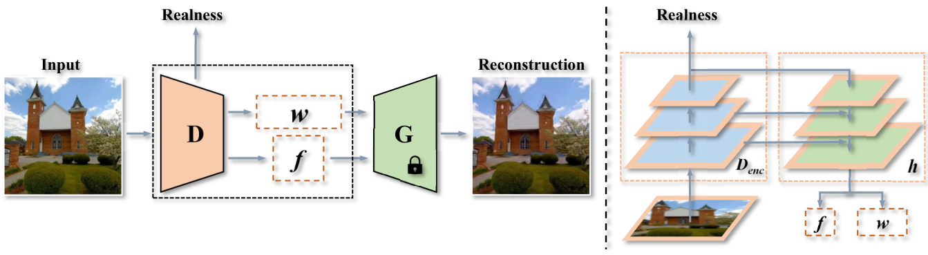
This work offers a different perspective on GAN improvement. In particular, we propose a new adversarial paradigm where G is assigned a new role, i.e., playing as the referee as well to guide D. Recall that producing realistic images usually requires $G$ to generate all-level concepts adequately. Nevertheless, due to the asymmetrical status of G and D, D is able to tell apart the real and synthesized data merely from limited discriminative regions wang2021eqgan. We, therefore, would like to encourage D to extract as much information from an image as possible, such that the features learned by D could be rendered back to the input with a frozen G, as in Fig. 1. That is, D is enforced to align with the view of G (i.e. focusing on the entire image region) instead of learning freely for domain classification.

Our method is termed as GLeaD because we propose to assign D a generator-leading task. In particular, given a real or synthesized image, the discriminator would deliver extra spatial representations and latent representations that are then fed into a frozen generator to reproduce the original image. Reconstruction loss (perceptual loss is adopted in practice) penalties the difference between the input image and the reconstructed image and derives gradients from updating the parameters of the discriminator. Moreover, comprehensive experiments are then conducted on various datasets, demonstrating the effectiveness of the proposed method. Particularly, our method improves Frechet Inception Distance (FID) fid from 4.30 to 2.55 on LSUN Bedroom and 4.04 to 2.82 on LSUN Church. We also manage to improve Recall kynkaanniemi2019improvedpr largely (56%) from 0.25 to 0.39 on LSUN Bedroom. In addition, thorough ablation studies also suggest that applying generator-leading tasks to require D to reconstruct only real or fake images could boost synthesis quality. While a larger improvement would be gained if both real and synthesized images were incorporated. Last but not least, experimental results in Sec. 4 reveal that our method can indeed boost the fairness between G and D as well as improve the spatial attention of D.

2 Related Work

Generative adversarial networks. As one of the popular paradigms for generative models, generative adversarial networks (GANs) goodfellow2014gan have significantly advanced image synthesis mirza2014conditional; radford2015unsupervised; gulrajani2017improved; brock2018biggan; karras2017progressive; karras2019stylegan; karras2020stylegan2; karras2020training; liu2021FastGAN; karras2021alias; esser2021taming, as well as various tasks like image manipulation shen2020interfacegan; harkonen2020ganspace; tov2021designing; patashnik2021styleclip; wu2021stylespace; zhu2021low, image translation isola2017image; liu2017unsupervised; zhu2017cyclegan; tang2020xinggan; choi2020stargan; wan2020bringing, image restoration agustsson2019generative; gu2020image; pan2021exploiting; wang2021towards, 3D-aware image synthsis zhou2021cips; chan2021pi; gu2021stylenerf; xu2022volumeGAN; shi20223daware, and talking head generation wu2018reenactgan; hong2022depth; yin2022styleheat. In the traditional setting of GAN training, D serves as the referee of synthesis quality and thus tends to dominate the competition. As a result, in practice D can always tell the real and fake samples apart and the equilibrium between G and D turns out hard to be achieved as expected goodfellow2014gan; arjovsky2017wgan. Some earlier work arjovsky2017wgan; berthelot2017began; fedus2017many tries to boost GAN equilibrium to stabilize GAN training and improve synthesis quality. Recently, EqGAN-SA wang2021eqgan proposes to boost GAN equilibrium by raising the spatial awareness of G. Concretely, the spatial attention of D is utilized to supervise and strengthen G. While our method forces D to fulfill a reconstruction task provided by G without improving the capacity of G for the first time. To learn useful feature representations with weak supervision, BiGAN donahue2016bigan proposes to learn an encoder, to project real samples back into GAN latent space in addition to the original G and D. And D is required to discriminate samples jointly in data and latent space. In this way, the well-trained encoder could serve as a feature extractor in a weak-supervised training manner. Differently, we directly adopt D to extract features of both real and synthesized samples to reconstruct them with G for a fairer setting instead of representation learning.

Improving GANs with the enhanced discriminator. Considering D largely dominates the competition with G, many prior works attempt to boost synthesis quality by improving D. Jolicoeur employs a relativistic discriminator jolicoeur2018relativistic to estimate the probability that the given real data is more realistic than fake data for better training stability and synthesis quality. Yang et al. yang2021insgen propose to improve D representation by additionally requiring D to distinguish every individual real and fake image. Kumari et al. kumari2022ensembling propose to ensemble selected backbones pre-trained on visual understanding tasks in addition to the original D as a strengthened D. The effect of various capacity of discriminator on training a generator is also investigated in yang2022improving. Based on the finding of OASIS sushko2020oasis that dense supervision such as segmentation labels could improve the representation of D in conditional synthesis, GGDR lee2022ggdr leverages the feature map of G to supervise the output features of D for unconditional synthesis. However, different from the discrimination process, G does not backward any gradient to D in this work. Contrasted with GGDR, our method aims at a fairer setting rather than gaining more supervision for D. Also, our D receives gradients from G, leading to fairer competition.

Image reconstruction with GANs. GAN inversion xia2022gan aims to reconstruct the input image with a pre-trained GAN generator. Mainstream GAN inversion methods include predicting desirable latent codes corresponding to the images through learning an encoder pidhorskyi2020alae; zhu2020idinvert; richardson2021pSp; tov2021e4e; alaluf2021restyle or optimization image2stylegan; abdal2020image2stylegan++; roich2021pivotal; creswell2018inverting; gu2020image; pan2020dgp. Most work chooses to predict latent codes in the native latent space of StyleGAN such as $\mathcal{Z}$ , $\mathcal{W}$ or $\mathcal{W+}$ . Recently there are also some work bai2022high; kang2021bdinvert extending the latent space or fine-tuing dinh2022hyperinverter; alaluf2022hyperstyle the generator for better reconstruction. Note that although our method could achieve image reconstruction with the well-trained D and G, our motivation lies in boosting generative quality by making G assign the generator-leading reconstruction task to D, instead of the reconstruction performance. Another significant difference lies in that we adopt D to extract representative features for reconstruction, which is simultaneously trained with G, while in GAN inversion the feature extractor (namely the encoder) is learned based on a pre-trained G.

3 Method

As mentioned before, it seems to be unfair that a discriminator (D) competes against a generator (G) since D does not only join the two-player game as a player but also guides the learning of G, namely serves as a referee for G. Section 3.1 presents the vanilla formulation. To chase a fairer game, Section 3.2 introduces a new adversarial paradigm GLeaD that assigns a new generator-leading task for D which in turn is judged by G.

3.1 Preliminary

GAN usually consists of two components: a generator $G(\cdot)$ and a discriminator $D(\cdot)$ . The former aims at mapping a random latent code ${\rm\bf z}$ to an image, while the latter learns to distinguish the synthesized image $G({\rm\bf z})$ from the real one ${\rm\bf x}$ . These two networks compete with each other and are jointly optimized with the learning objectives as follows:

	$\displaystyle{\mathcal{L}}_{G}$	$\displaystyle=-\mathbb{E}_{{\rm\bf z}\in\mathcal{Z}}[\log(D(G({\rm\bf z})))],$		(1)
	$\displaystyle{\mathcal{L}}_{D}$	$\displaystyle=-\mathbb{E}_{{\rm\bf x}\in\mathcal{X}}[\log(D({\rm\bf x}))]-\mathbb{E}_{{\rm\bf z}\in\mathcal{Z}}[\log(1-D(G({\rm\bf z})))],$		(2)

where $\mathcal{Z}$ and $\mathcal{X}$ denote a pre-defined latent distribution and data distribution respectively.

Ideally, the optimal solution is that G manages to reproduce the realistic data distribution while D is not able to tell the real and synthesized samples apart goodfellow2014gan. However, during the iterative training of the generator and discriminator, there exists an unfair competition since D plays the player and referee roles simultaneously. Thus the ideal solution is hard to be achieved in practice wang2021eqgan; farnia2020gans.

3.2 Generator-leading Task

Considering the unfair division of labor in this two-player game, we turn to assign a new role to G that could supervise the learning of D in turn. Recall that the target of generation is to produce realistic samples which usually requires all concepts well-synthesized. However, it is suggested wang2021eqgan that the most discriminative regions of given real or synthesized images are sufficient for domain classification. Therefore, we propose a generator-leading task that enforces D to extract as many representative features as possible to retain adequate information that could reconstruct a given image through a frozen generator, as described in Fig. 2 and Algorithm 1. Note that we empirically validate that requiring D to extract spatial representations is essential to improve synthesis quality in Section 4.3. Taking StyleGAN2 karras2020stylegan2 as an example, we will introduce the detailed instantiations in the following context.

Extracting representations through D. The original D of StyleGAN is a convolutional network composed of a series of downsampling convolution layers. To make it convenient, the backbone network of the original D (namely, parts of D except the final head predicting realness score) is denoted as $D_{enc}$ in the following statement. In order to predict the representative features of a given image while retaining various information from low-level to high-level, we additionally affiliate $D_{enc}$ with a decoder $h(\cdot)$ to construct our new D with a multi-level feature pyramid lin2017fpn. Based on such feature hierarchy ending with a convolutional head, spatial representations ${\rm\bf f}$ and latent representations ${\rm\bf w}$ are predicted respectively. In particular, the newly-attached parts over the backbone adopt convolution layers with the kernel size of $1\times 1$ . This is because the crucial part in D that influences the synthesis quality of G is the backbone while introducing too many parameters for $h$ will encourage the optimization to focus on this reconstruction branch (decoder). Moreover, considering the residual architecture of G, the spatial representation ${\rm\bf f}$ consists of a low-level feature and a high-level one in total. More details are available in Supplementary Material. Therefore, given one real image ${\rm\bf x}$ or a synthesized one $G({\rm\bf z})$ , the corresponding representative features could be obtained by:

	$\displaystyle{\rm\bf f}_{real},{\rm\bf w}_{real}$	$\displaystyle=h(D_{enc}({\rm\bf x})),$		(3)
	$\displaystyle{\rm\bf f}_{fake},{\rm\bf w}_{fake}$	$\displaystyle=h(D_{enc}(G({\rm\bf z}))).$		(4)

Reconstructing images via a frozen G. For a fair comparison, the generator of the original StyleGAN2 is adopted without any modification, which stacks a series of convolutional “synthesis blocks”. Notably, the StyleGAN2 generator is designed with a residual architecture, which synthesizes images progressively from a lower resolution to the higher one. For instance, the $16\times 16$ synthesized result of the synthesis block corresponding to a lower resolution is firstly upsampled to $32\times 32$ , and then the $32\times 32$ synthesis block only predicts the residual between the upsampled result and the desirable $32\times 32$ image. As mentioned before, our predicted spatial representations indeed contain two features that could serve as the basis and the residual respectively. And the latent representation is sent to the synthesis blocks to modulate the features to generate the final output just as in karras2019stylegan; karras2020stylegan2. Such that, the reconstructed images could be derived from:

	$\displaystyle{\rm\bf x}_{real}^{\prime}$	$\displaystyle=G({\rm\bf f}_{real},{\rm\bf w}_{real}),$		(5)
	$\displaystyle{\rm\bf x}_{fake}^{\prime}$	$\displaystyle=G({\rm\bf f}_{fake},{\rm\bf w}_{fake}),$		(6)

where G is fully frozen.

Reconstruction loss.

Algorithm 1 GAN training with the proposed generator-leading task.

G

and our

D

(including

h

) that are initialized with random parameters. Training data

\{\rm\bf x_{i}\}

T

: maximum number of training iterations.

3: for

t=1

T

4: Sample

{\rm\bf z}\sim\mathbb{P}(\mathcal{Z})

\triangleright

Begin training of

G

5: Update

G

with Eq. 1

6: Sample

{\rm\bf z}\sim\mathbb{P}(\mathcal{Z})

\triangleright

Begin training of

D

7: Reconstruct

G({\rm\bf z})

with Eq. 4 and Eq. 6

8: Sample

{\rm\bf x}\sim\{\rm\bf x_{i}\}

9: Reconstruct

{\rm\bf x}

with Eq. 3 and Eq. 5

10: Discriminate images by

D(G({\rm\bf z}))

and

D({\rm\bf x})

11: Update

D

with Eq. 2, Eq. 7, and Eq. 9

12: end for

13:

G

with best training set FID.

After gathering the reconstructed real and synthesized images, we could easily penalize the differences between the original images and reconstructed ones. Here, perceptual loss zhang2018perceptual ${\mathcal{L}}_{per}$ is adopted as the loss function:

\displaystyle{\mathcal{L}}_{rec}=\lambda_{1}{\mathcal{L}}_{per}({\rm\bf x},{\rm\bf x}_{real}^{\prime})+\lambda_{2}{\mathcal{L}}_{per}(G({\rm\bf z}),{\rm\bf x}_{fake}^{\prime}),

(7)

where $\lambda_{1}$ and $\lambda_{2}$ denote the weights for different terms. Note that setting one weight as zero is identical to disabling the reconstruction tasks on real/synthesized images, which may deteriorate the synthesis performance to some extent. Our final algorithm is summarized as in Algorithm 1.

Full objective. With the updated D architecture and the generator-leading task, the discriminator and generator are jointly optimized with

	$\displaystyle{\mathcal{L}}_{G}^{\prime}$	$\displaystyle={\mathcal{L}}_{G},$		(8)
	$\displaystyle{\mathcal{L}}_{D}^{\prime}$	$\displaystyle={\mathcal{L}}_{D}+{\mathcal{L}}_{rec}.$		(9)

4 Experiments

Table 1: Comparisons on FFHQ karras2019stylegan, LSUN Bedroom and LSUN Church yu2015lsun. Our method improves StyleGAN2 karras2020stylegan2 in large datasets in terms of FID fid and recall. P and R denote precision and recall kynkaanniemi2019improvedpr. Lower FID and higher precision and recall indicate better performance. The bold numbers indicate the best metrics for each dataset. The blue numbers in the brackets indicate the improvements.

Method	FFHQ karras2019stylegan			LSUN Bedroom yu2015lsun			LSUN Church yu2015lsun
Method	FID $\downarrow$	P $\uparrow$	R $\uparrow$	FID $\downarrow$	P $\uparrow$	R $\uparrow$	FID $\downarrow$	P $\uparrow$	R $\uparrow$
UT bond2021unleashing	6.11	0.73	0.48	-	-	-	4.07	0.71	0.45
Polarity humayun2022polarity	-	-	-	-	-	-	3.92	0.61	0.39
StyleGAN2 karras2020stylegan2	3.79	0.68	0.44	4.30	0.59	0.25	4.04	0.58	0.40
Ours	3.24 ( $-$ 0.55)	0.69	0.47	2.55 ( $-$ 1.75)	0.62	0.39	2.82 ( $-$ 1.22)	0.62	0.43
GGDR lee2022ggdr	3.25	0.66	0.51	3.71	0.62	0.33	2.81	0.61	0.46
Ours*	2.90 ( $-$ 0.35)	0.69	0.50	2.72 ( $-$ 0.99)	0.62	0.37	2.15 ( $-$ 0.66)	0.61	0.48

We conduct extensive experiments on various benchmark datasets to demonstrate the effectiveness of the proposed method and the superiority of the specific settings. The subsections are arranged as follows: Section 4.1 introduces our detailed experiment settings. In Table 1 we demonstrate the qualitative and quantitative superiority of GLeaD . Section 4.3 includes comprehensive ablation studies of the designed components. Then we visualize the realness score curves of D to validate the improvement of fairness in Section 4.4. At last, we provide qualitative reconstruction results and validate the improvement of D’s spatial attention respectively in Section 4.5 and Section 4.6.

4.1 Experimental Setup

Datasets. We conduct experiments on FFHQ karras2019stylegan consisting of 70K high-resolution portraits for face synthesis. We also adopt the training set of LSUN Bedroom and Church yu2015lsun respectively for indoor and outdoor scene synthesis, which respectively contains about 126K and 3M $256\times 256$ images.

Evaluation. We mainly adopt the prevalent Frechet Inception Distance (FID) fid for evaluation. Precision & Recall (P&R) kynkaanniemi2019improvedpr is also adopted as the supplement of FID for more grounded evaluation. In particular, we calculate FID and P&R between all the real samples and 50K synthesized ones for experiments on FFHQ and LSUN Church. While for LSUN Bedroom we calculate FID and P&R between 50K real samples and 50K synthesized ones because feature extracting of 3M samples is rather costly.

Other settings. For all the baseline and our models, on FFHQ we keep training the model until D has been shown 25M images with mirror augmentation. While models on LSUN Church and Bedroom are trained until 50M images have been shown to D for more sufficient convergence. We adopt VGG simonyan2014vgg as the pre-trained feature extractor for perceptual loss calculation. As for the loss weights, we set $\lambda_{1}$ = 10 and $\lambda_{2}$ = 3.

4.2 Main Results

Quantitative comparisons. In order to compare our GLeaD against prior works, e.g., UT bond2021unleashing, Polarity humayun2022polarity, and StyleGAN2 karras2020stylegan2, we calculate the FID and Precision and Recall kynkaanniemi2019improvedpr (P & R) to measure the synthesis. In particular, Precision and Recall could reflect the synthesis quality and diversity to some extent. Moreover, considering that recent work GGDR lee2022ggdr also leverages the G to enhance the representations of D, we further incorporate it with our method to check whether exists a consistent gain.

Table 1 presents the results. From the perspective of FID, our direct baseline StyleGAN2 could be substantially improved with the proposed GLeaD, outperforming other approaches by a clear margin. These results strongly demonstrate the effectiveness of our GLeaD. Moreover, combined with GGDR (Ours* in the table), our GLeaD could further introduce significant gains, achieving new state-of-the-art performance on various datasets. Namely, the proposed GLeaD could be compatible with the recent work GGDR that also considers improving D through G.

Regarding Precision and Recall, clear gains are also observed on multiple benchmarks. Importantly, the improvements mainly come from the Recall side, i.e., the synthesis diversity is further improved. This matches our motivation that the generator-leading task could further urge D to extract more representative features rather than focus on the limited discriminative regions. As a result, G has to synthesize images with a variety of modes to fool D in turn. Moreover, the diversity is significantly improved in the LSUN bedrooms from 0.25 to 0.39 (56%). This may imply that our GLeaD could continuously benefit from the larger-scale reconstruction task, which we leave in future studies.

Qualitative results. Fig. 3 presents the synthesized samples by our GLeaD. The models are respectively trained on FFHQ, LSUN Bedroom, and LSUN Church. Obviously, all models could generate images with desirable quality and coverage.

Computational costs. We evaluate the proposed model in terms of parameter amount and inference time. The specific results could be found in Supplementary Material.

4.3 Ablation Studies

Table 2: Ablation studies on the loss weights

\lambda_{1}

and

\lambda_{2}

. The numbers in bold indicate the best FID in each sub-table.

$\lambda_{1}$	$\lambda_{2}$	FID
0	0	4.04
100	0	331
10	0	3.10
1	0	3.27

$\lambda_{1}$	$\lambda_{2}$	FID
0	10	3.32
10	10	3.15
10	3	2.82
10	1	2.85

Table 3: Ablation studies on the resolution of

{\rm\bf f}

. The upper line indicates the resolution settings and the bottom line concludes the corresponding FID performance. The number in bold indicates the best FID in the table.

Baseline	$1\times 1$	$8\times 8$	$16\times 16$	$32\times 32$	$64\times 64$
4.04	4.68	3.27	3.01	2.82	2.88

Constraint strength. Here we ablate the specific target of the proposed generator-leading task on LSUN Church. Recall that we have $\lambda_{1}$ and $\lambda_{2}$ that respectively control the constraint strength when reconstructing real and fake images in Eq. 7. As shown in the left sub-table of Table 2, we first set $\lambda_{1}=\lambda_{2}=0$ to get the baseline performance. Then we set $\lambda_{2}$ as 0 and explore a proper $\lambda_{1}$ for only reconstructing real images. Experiments suggest that an overlarge weight like 100 will make the proposed task interfere with the adversarial training and the model cannot converge. And 10 turns out to be a proper choice for $\lambda_{1}$ , improving FID from 4.04 to 3.10. The results incorporating the reconstruction of fake images are demonstrated in the sub-table on the right of Table 2. We first set $\lambda_{1}=0$ and $\lambda_{2}=10$ to validate that merely reconstructing fake images benefits the synthesis quality. Then we try to find an appropriate $\lambda_{2}$ when the reconstruction of real images has been incorporated in the task ( $\lambda_{1}=10$ ). Through the aforementioned experiments, reconstructing both real and fake images when $\lambda_{1}=10$ and $\lambda_{2}=3$ turns out to be the best strategy.

Resolution of ${\rm\bf f}$ . Recall that we require D to extract spatial features ${\rm\bf f}$ as the basis of the image reconstruction. And the predicted latent codes ${\rm\bf w}$ modulate the latter features of G to generate the reconstructed image based on ${\rm\bf f}$ . Here we conduct ablation studies on the resolution of ${\rm\bf f}$ on LSUN Church. As in Table 3, extracting ${\rm\bf f}$ whose resolution is $32\times 32$ brings the best synthesis quality. And $1\times 1$ in the table indicates the setting where D only predicts latent codes $w$ without spatial dimension. Notably, the model performance under this setting is even inferior than the baseline, suggesting the necessity of extracting spatial features.

4.4 Validation of the Fairer Game

Recall that aiming to improve the synthesis quality through a fairer setting between G and D, we provide the generator-leading task for D to extract representative features adequate for reconstruction. Thus we validate the boosted fairness in this subsection through experiments.

Following wang2021eqgan, we visualize the mean score in terms of realness extracted by discriminators throughout the training process on LSUN Bedroom. Note that the curves are smoothed with exponentially weighted averages hunter1986exponentially for clearer understanding. The top of Fig. 4 describes the visualization results for the real images while the bottom includes score curves for the synthesized images. The colors of the curves indicate various settings for training GANs, as labeled on the right of Fig. 4. From the aforementioned figure, it can be found that equipped with our generator-leading task, the absolute score values of our methods become smaller than the baseline. While GGDR lee2022ggdr (the red curve) just maintains and even enlarges the gap between the absolute values and zero compared to the baseline, though it can improve FID.

We can thus draw a conclusion that with the aid of the generator-leading task, it becomes much more challenging for D to distinguish the real and fake samples. In other words, GLeaD can improve the fairness between G and D, as well as the synthesis quality. On the contrary, the effectiveness of GGDR is not brought by the improvement of fairness, which emphasizes the viewpoint that, in order to boost fairness between G and D, it is necessary to pass gradients of G to D like our method.

4.5 Reconstruction Results

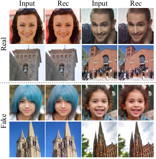
Recall that we instantiate the generator-leading task as a reconstruction task. In this subsection, we provide reconstruction results of real and fake images with the well-trained D and G. To explore the reconstruction ability of D more accurately, we provide it with unseen real and synthesized images to extract features. These features are then fed into the corresponding G to reconstruct the images inputted to D, as in the training stage. As mentioned in Section 4.1, we train GANs on FFHQ for the face domain and training set of LSUN Church for outdoor scenes. Thus, here we randomly sample real images from CelebA-HQ progan; liu2015faceattributes (another widely-used face dataset) and the validation set of LSUN Church. Fake images are sampled with the generators corresponding to the tested discriminators.

As shown in Fig. 5, though some out-of-domain objects (e.g., crowds in Church) and high-frequency details (e.g., teeth of the child) are not perfectly well-reconstructed, our well-trained discriminator manages to extract representative features and reproduce the input real and fake images with G. This indicates that our D could learn features aligned with the domain of G, matching our motivation.

4.6 Spatial Attention Visualization for D

We also visualize the spatial attention of the well-trained discriminators with the help of GradCAM selvaraju2017grad. As mentioned in Section 1, we expect D to avoid focusing on some limited regions or objects, by extracting spatial representative features. Here, the discriminators of the baseline and our method are chosen to validate the improvement in terms of spatial attention. Considering the discriminators have been fully trained, we pick some generated images with unacceptable artifacts, expecting D aware of these regions with artifacts. For fair comparison, G of GGDR is adopted to synthesize the images rather than the baseline or ours. The spatial attention maps are demonstrated in Fig. 6, note that we pick the gradient map with a relatively higher resolution (64 $\times$ 64) because it is more spatially aligned with the original image than an abstract one (e.g., 8 $\times$ 8).

As in Fig. 6, the provided fake images contain various kinds of unpleasant artifacts. The background of the portrait is full of unidentified filamentous artifacts. And there is a weird object on the bed in the bedroom picture. Compared with the baseline D, our D pays much more attention to the artifacts instead of focusing on the face and the bed, which are well synthesized as the subject. Recall that under the generator-leading task, D is forced to extract representative spatial features to faithfully reconstruct the inputs. To achieve this additional task, the backbone of D (namely $D_{enc}$ ) is naturally forced to learn a much stronger representation than only fulfilling the binary classification task. Moreover, it is suggested that the strengthened representation of D is strong enough to better detect the generated artifacts. In contrast, the red regions in the attention map of the baseline are mainly distributed on the face or bed, which means D pays more attention to the subject of the training set, even though there are artifacts generated by G. Naturally, D’s success in detecting and penalizing the artifacts will improve the synthesis capability of G. And this could serve as one of the reasons why GLeaD can boost the synthesis quality of GANs.

5 Conclusion

Generative adversarial network (GAN) is formulated as a two-player game between a generator (G) and a discriminator (D). In order to establish a fairer game setting between G and D, we propose a new adversarial paradigm additionally assigning D a generator-leading task, which is termed as GLeaD. Specifically, we urge D to extract adequate features from the input real and fake images. These features should be representative enough that G can reconstruct the original inputs with them. As a result, D is forced to learn a stronger representation aligned with G instead of learning and discriminating freely. Thus the unfairness between G and D could be alleviated. Massive experiments demonstrate GLeaD can significantly improve the synthesis quality over the baseline.

References

(1) Rameen Abdal, Yipeng Qin, and Peter Wonka. Image2StyleGAN++: How to edit the embedded images? In IEEE Conf. Comput. Vis. Pattern Recog., 2020.
(2) Eirikur Agustsson, Michael Tschannen, Fabian Mentzer, Radu Timofte, and Luc Van Gool. Generative adversarial networks for extreme learned image compression. In IEEE Conf. Comput. Vis. Pattern Recog., pages 221–231, 2019.
(3) Yuval Alaluf, Or Patashnik, and Daniel Cohen-Or. ReStyle: A residual-based StyleGAN encoder via iterative refinement. In Int. Conf. Comput. Vis., 2021.
(4) Yuval Alaluf, Omer Tov, Ron Mokady, Rinon Gal, and Amit Bermano. Hyperstyle: StyleGAN inversion with hypernetworks for real image editing. In IEEE Conf. Comput. Vis. Pattern Recog., 2022.
(5) Martin Arjovsky, Soumith Chintala, and Léon Bottou. Wasserstein generative adversarial networks. In Int. Conf. Mach. Learn., 2017.
(6) Qingyan Bai, Yinghao Xu, Jiapeng Zhu, Weihao Xia, Yujiu Yang, and Yujun Shen. High-fidelity GAN inversion with padding space. In Eur. Conf. Comput. Vis., 2022.
(7) David Berthelot, Thomas Schumm, and Luke Metz. Began: Boundary equilibrium generative adversarial networks. In arXiv preprint arXiv:1703.10717, 2017.
(8) Sam Bond-Taylor, Peter Hessey, Hiroshi Sasaki, Toby P Breckon, and Chris G Willcocks. Unleashing transformers: Parallel token prediction with discrete absorbing diffusion for fast high-resolution image generation from vector-quantized codes. In Eur. Conf. Comput. Vis., 2022.
(9) Andrew Brock, Jeff Donahue, and Karen Simonyan. Large scale GAN training for high fidelity natural image synthesis. In Int. Conf. Learn. Represent., 2019.
(10) Eric R Chan, Marco Monteiro, Petr Kellnhofer, Jiajun Wu, and Gordon Wetzstein. pi-gan: Periodic implicit generative adversarial networks for 3d-aware image synthesis. In IEEE Conf. Comput. Vis. Pattern Recog., 2021.
(11) Yunjey Choi, Youngjung Uh, Jaejun Yoo, and Jung-Woo Ha. Stargan v2: Diverse image synthesis for multiple domains. In IEEE Conf. Comput. Vis. Pattern Recog., 2020.
(12) Antonia Creswell and Anil Anthony Bharath. Inverting the generator of a generative adversarial network. IEEE Trans. Neur. Network. Learn. Syst., 2018.
(13) Tan M Dinh, Anh Tuan Tran, Rang Nguyen, and Binh-Son Hua. Hyperinverter: Improving StyleGAN inversion via hypernetwork. In IEEE Conf. Comput. Vis. Pattern Recog., 2022.
(14) Jeff Donahue, Philipp Krähenbühl, and Trevor Darrell. Adversarial feature learning. In Int. Conf. Learn. Represent., 2017.
(15) Patrick Esser, Robin Rombach, and Bjorn Ommer. Taming transformers for high-resolution image synthesis. In IEEE Conf. Comput. Vis. Pattern Recog., 2021.
(16) Farzan Farnia and Asuman Ozdaglar. Do GANs always have nash equilibria? In Int. Conf. Mach. Learn., 2020.
(17) William Fedus, Mihaela Rosca, Balaji Lakshminarayanan, Andrew M Dai, Shakir Mohamed, and Ian Goodfellow. Many paths to equilibrium: GANs do not need to decrease a divergence at every step. In Int. Conf. Learn. Represent., 2018.
(18) Ian Goodfellow, Jean Pouget-Abadie, Mehdi Mirza, Bing Xu, David Warde-Farley, Sherjil Ozair, Aaron Courville, and Yoshua Bengio. Generative adversarial networks. In Adv. Neural Inform. Process. Syst., 2014.
(19) Jiatao Gu, Lingjie Liu, Peng Wang, and Christian Theobalt. Stylenerf: A style-based 3d-aware generator for high-resolution image synthesis. In Int. Conf. Learn. Represent., 2022.
(20) Jinjin Gu, Yujun Shen, and Bolei Zhou. Image processing using multi-code GAN prior. In IEEE Conf. Comput. Vis. Pattern Recog., 2020.
(21) Ishaan Gulrajani, Faruk Ahmed, Martin Arjovsky, Vincent Dumoulin, and Aaron C Courville. Improved training of wasserstein gans. In Adv. Neural Inform. Process. Syst., 2017.
(22) Erik Härkönen, Aaron Hertzmann, Jaakko Lehtinen, and Sylvain Paris. Ganspace: Discovering interpretable GAN controls. In Adv. Neural Inform. Process. Syst., 2020.
(23) Martin Heusel, Hubert Ramsauer, Thomas Unterthiner, Bernhard Nessler, and Sepp Hochreiter. GANs trained by a two time-scale update rule converge to a local nash equilibrium. In Adv. Neural Inform. Process. Syst., 2017.
(24) Fa-Ting Hong, Longhao Zhang, Li Shen, and Dan Xu. Depth-aware generative adversarial network for talking head video generation. In IEEE Conf. Comput. Vis. Pattern Recog., 2022.
(25) Ahmed Imtiaz Humayun, Randall Balestriero, and Richard Baraniuk. Polarity sampling: Quality and diversity control of pre-trained generative networks via singular values. In IEEE Conf. Comput. Vis. Pattern Recog., 2022.
(26) J Stuart Hunter. The exponentially weighted moving average. Journal of quality technology, 18(4), 1986.
(27) Phillip Isola, Jun-Yan Zhu, Tinghui Zhou, and Alexei A Efros. Image-to-image translation with conditional adversarial networks. In IEEE Conf. Comput. Vis. Pattern Recog., 2017.
(28) Jongheon Jeong and Jinwoo Shin. Training GANs with stronger augmentations via contrastive discriminator. In Int. Conf. Learn. Represent., 2021.
(29) Alexia Jolicoeur-Martineau. The relativistic discriminator: a key element missing from standard GAN. In Int. Conf. Learn. Represent., 2019.
(30) Kyoungkook Kang, Seongtae Kim, and Sunghyun Cho. GAN inversion for out-of-range images with geometric transformations. In IEEE Conf. Comput. Vis. Pattern Recog., 2021.
(31) Tero Karras, Timo Aila, Samuli Laine, and Jaakko Lehtinen. Progressive growing of GANs for improved quality, stability, and variation. In Int. Conf. Learn. Represent., 2018.
(32) Tero Karras, Timo Aila, Samuli Laine, and Jaakko Lehtinen. Progressive growing of GANs for improved quality, stability, and variation. In Int. Conf. Learn. Represent., 2018.
(33) Tero Karras, Miika Aittala, Janne Hellsten, Samuli Laine, Jaakko Lehtinen, and Timo Aila. Training generative adversarial networks with limited data. In Adv. Neural Inform. Process. Syst., 2020.
(34) Tero Karras, Miika Aittala, Janne Hellsten, Samuli Laine, Jaakko Lehtinen, and Timo Aila. Training generative adversarial networks with limited data. In Adv. Neural Inform. Process. Syst., volume 33, 2020.
(35) Tero Karras, Miika Aittala, Samuli Laine, Erik Härkönen, Janne Hellsten, Jaakko Lehtinen, and Timo Aila. Alias-free generative adversarial networks. In Adv. Neural Inform. Process. Syst., volume 34, 2021.
(36) Tero Karras, Samuli Laine, and Timo Aila. A style-based generator architecture for generative adversarial networks. In IEEE Conf. Comput. Vis. Pattern Recog., 2019.
(37) Tero Karras, Samuli Laine, Miika Aittala, Janne Hellsten, Jaakko Lehtinen, and Timo Aila. Analyzing and improving the image quality of StyleGAN. In IEEE Conf. Comput. Vis. Pattern Recog., 2020.
(38) Nupur Kumari, Richard Zhang, Eli Shechtman, and Jun-Yan Zhu. Ensembling off-the-shelf models for GAN training. In IEEE Conf. Comput. Vis. Pattern Recog., 2022.
(39) Tuomas Kynkäänniemi, Tero Karras, Samuli Laine, Jaakko Lehtinen, and Timo Aila. Improved precision and recall metric for assessing generative models. In Adv. Neural Inform. Process. Syst., 2019.
(40) Gayoung Lee, Hyunsu Kim, Junho Kim, Seonghyeon Kim, Jung-Woo Ha, and Yunjey Choi. Generator knows what discriminator should learn in unconditional GANs. In Eur. Conf. Comput. Vis., 2022.
(41) Tsung-Yi Lin, Piotr Dollár, Ross Girshick, Kaiming He, Bharath Hariharan, and Serge Belongie. Feature pyramid networks for object detection. In IEEE Conf. Comput. Vis. Pattern Recog., 2017.
(42) Bingchen Liu, Yizhe Zhu, Kunpeng Song, and Ahmed Elgammal. Towards faster and stabilized GAN training for high-fidelity few-shot image synthesis. In Int. Conf. Learn. Represent., 2021.
(43) Ming-Yu Liu, Thomas Breuel, and Jan Kautz. Unsupervised image-to-image translation networks. In Adv. Neural Inform. Process. Syst., 2017.
(44) Ziwei Liu, Ping Luo, Xiaogang Wang, and Xiaoou Tang. Deep learning face attributes in the wild. In Int. Conf. Comput. Vis., 2015.
(45) Mehdi Mirza and Simon Osindero. Conditional generative adversarial nets. arXiv preprint arXiv:1411.1784, 2014.
(46) Xingang Pan, Xiaohang Zhan, Bo Dai, Dahua Lin, Chen Change Loy, and Ping Luo. Exploiting deep generative prior for versatile image restoration and manipulation. In Eur. Conf. Comput. Vis., 2020.
(47) Xingang Pan, Xiaohang Zhan, Bo Dai, Dahua Lin, Chen Change Loy, and Ping Luo. Exploiting deep generative prior for versatile image restoration and manipulation. IEEE Trans. Pattern Anal. Mach. Intell., 2021.
(48) Or Patashnik, Zongze Wu, Eli Shechtman, Daniel Cohen-Or, and Dani Lischinski. Styleclip: Text-driven manipulation of StyleGAN imagery. In Int. Conf. Comput. Vis., 2021.
(49) Stanislav Pidhorskyi, Donald A Adjeroh, and Gianfranco Doretto. Adversarial latent autoencoders. In IEEE Conf. Comput. Vis. Pattern Recog., 2020.
(50) Alec Radford, Luke Metz, and Soumith Chintala. Unsupervised representation learning with deep convolutional generative adversarial networks. In Int. Conf. Learn. Represent., 2016.
(51) Abdal Rameen, Qin Yipeng, and Wonka Peter. Image2StyleGAN: How to embed images into the StyleGAN latent space? In Int. Conf. Comput. Vis., 2019.
(52) Elad Richardson, Yuval Alaluf, Or Patashnik, Yotam Nitzan, Yaniv Azar, Stav Shapiro, and Daniel Cohen-Or. Encoding in style: a StyleGAN encoder for image-to-image translation. In IEEE Conf. Comput. Vis. Pattern Recog., 2021.
(53) Daniel Roich, Ron Mokady, Amit H Bermano, and Daniel Cohen-Or. Pivotal tuning for latent-based editing of real images. ACM Trans. Graph., 2021.
(54) Ramprasaath R Selvaraju, Michael Cogswell, Abhishek Das, Ramakrishna Vedantam, Devi Parikh, and Dhruv Batra. Grad-cam: Visual explanations from deep networks via gradient-based localization. In IEEE Conf. Comput. Vis. Pattern Recog., 2017.
(55) Yujun Shen, Jinjin Gu, Xiaoou Tang, and Bolei Zhou. Interpreting the latent space of GANs for semantic face editing. In IEEE Conf. Comput. Vis. Pattern Recog., 2020.
(56) Zifan Shi, Yujun Shen, Jiapeng Zhu, Dit-Yan Yeung, and Qifeng Chen. 3d-aware indoor scene synthesis with depth priors. In Eur. Conf. Comput. Vis., 2022.
(57) Zifan Shi, Yinghao Xu, Yujun Shen, Deli Zhao, Qifeng Chen, and Dit-Yan Yeung. Improving 3d-aware image synthesis with a geometry-aware discriminator. In Adv. Neural Inform. Process. Syst., 2022.
(58) Karen Simonyan and Andrew Zisserman. Very deep convolutional networks for large-scale image recognition. In Int. Conf. Learn. Represent., 2015.
(59) Vadim Sushko, Edgar Schönfeld, Dan Zhang, Juergen Gall, Bernt Schiele, and Anna Khoreva. You only need adversarial supervision for semantic image synthesis. In Int. Conf. Learn. Represent., 2021.
(60) Hao Tang, Song Bai, Li Zhang, Philip HS Torr, and Nicu Sebe. Xinggan for person image generation. In Eur. Conf. Comput. Vis., pages 717–734. Springer, 2020.
(61) Omer Tov, Yuval Alaluf, Yotam Nitzan, Or Patashnik, and Daniel Cohen-Or. Designing an encoder for StyleGAN image manipulation. ACM Trans. Graph., 40(4):1–14, 2021.
(62) Omer Tov, Yuval Alaluf, Yotam Nitzan, Or Patashnik, and Daniel Cohen-Or. Designing an encoder for StyleGAN image manipulation. ACM Trans. Graph., 2021.
(63) Ziyu Wan, Bo Zhang, Dongdong Chen, Pan Zhang, Dong Chen, Jing Liao, and Fang Wen. Bringing old photos back to life. In IEEE Conf. Comput. Vis. Pattern Recog., 2020.
(64) Jianyuan Wang, Ceyuan Yang, Yinghao Xu, Yujun Shen, Hongdong Li, and Bolei Zhou. Improving GAN equilibrium by raising spatial awareness. In IEEE Conf. Comput. Vis. Pattern Recog., 2022.
(65) Xintao Wang, Yu Li, Honglun Zhang, and Ying Shan. Towards real-world blind face restoration with generative facial prior. In IEEE Conf. Comput. Vis. Pattern Recog., 2021.
(66) Wayne Wu, Yunxuan Zhang, Cheng Li, Chen Qian, and Chen Change Loy. Reenactgan: Learning to reenact faces via boundary transfer. In Eur. Conf. Comput. Vis., 2018.
(67) Zongze Wu, Dani Lischinski, and Eli Shechtman. Stylespace analysis: Disentangled controls for StyleGAN image generation. In IEEE Conf. Comput. Vis. Pattern Recog., 2021.
(68) Weihao Xia, Yulun Zhang, Yujiu Yang, Jing-Hao Xue, Bolei Zhou, and Ming-Hsuan Yang. GAN inversion: A survey. IEEE Trans. Pattern Anal. Mach. Intell., 2022.
(69) Yinghao Xu, Sida Peng, Ceyuan Yang, Yujun Shen, and Bolei Zhou. 3d-aware image synthesis via learning structural and textural representations. In IEEE Conf. Comput. Vis. Pattern Recog., 2022.
(70) Ceyuan Yang, Yujun Shen, Yinghao Xu, Deli Zhao, Bo Dai, and Bolei Zhou. Improving gans with a dynamic discriminator. In Adv. Neural Inform. Process. Syst., 2022.
(71) Ceyuan Yang, Yujun Shen, Yinghao Xu, and Bolei Zhou. Data-efficient instance generation from instance discrimination. In Adv. Neural Inform. Process. Syst., 2021.
(72) Fei Yin, Yong Zhang, Xiaodong Cun, Mingdeng Cao, Yanbo Fan, Xuan Wang, Qingyan Bai, Baoyuan Wu, Jue Wang, and Yujiu Yang. Styleheat: One-shot high-resolution editable talking face generation via pretrained StyleGAN. In Eur. Conf. Comput. Vis., 2022.
(73) Fisher Yu, Ari Seff, Yinda Zhang, Shuran Song, Thomas Funkhouser, and Jianxiong Xiao. Lsun: Construction of a large-scale image dataset using deep learning with humans in the loop. arXiv preprint arXiv:1506.03365, 2015.
(74) Richard Zhang, Phillip Isola, Alexei A Efros, Eli Shechtman, and Oliver Wang. The unreasonable effectiveness of deep features as a perceptual metric. In IEEE Conf. Comput. Vis. Pattern Recog., 2018.
(75) Peng Zhou, Lingxi Xie, Bingbing Ni, and Qi Tian. Cips-3d: A 3d-aware generator of GANs based on conditionally-independent pixel synthesis. arXiv preprint arXiv:2110.09788, 2021.
(76) Jiapeng Zhu, Ruili Feng, Yujun Shen, Deli Zhao, Zheng-Jun Zha, Jingren Zhou, and Qifeng Chen. Low-rank subspaces in GANs. In Adv. Neural Inform. Process. Syst., volume 34, 2021.
(77) Jiapeng Zhu, Yujun Shen, Deli Zhao, and Bolei Zhou. In-domain GAN inversion for real image editing. In Eur. Conf. Comput. Vis., 2020.
(78) Jun-Yan Zhu, Taesung Park, Phillip Isola, and Alexei A Efros. Unpaired image-to-image translation using cycle-consistent adversarial networks. In IEEE Conf. Comput. Vis. Pattern Recog., 2017.

Appendix

Appendix A Discriminator Network Structure

Recall that, our D includes a backbone $D_{enc}$ , a head predicting realness scores, and a decoder $h$ for predicting representative features $f$ and $w$ . Taking an image whose resolution is $256\times 256$ as an instance, the backbone $D_{enc}$ is first employed to extract features from the input image. The very last feature map of $4\times 4$ is sent to the scoring head to extract the realness score while the multi-level feature maps are sent to the decoder $h$ to predict the representative features adequate for G to reconstruct the original image. As described in the submission, the representative features consist of latent codes $w$ and the spatial representations $f$ , which include a low-level representation and a high-level representation. Recall that, these spatial representations will be sent to the fixed generator to serve as the basis of the reconstruction and will be modulated by latent codes to predict the final results. We illustrate the architectures of the three aforementioned components of D in Table 4, Table 5, and Table 6, respectively.

Table 4: Network structure of the backbone

D_{enc}

. The output size is with order

\{C\times H\times W\}

, where

C

H

, and

W

respectively denotes the channel dimension, height and weight of the output.

Stage	Block	Output Size
input	-	$3\times 256\times 256$
block₁	$\left[\begin{array}[]{c}\text{1$\times$1 $\mathtt{Conv}$, {128}}\\[-1.00006pt] \text{2$\times$3$\times$3 $\mathtt{Conv}$, {128}}\\[-1.00006pt] \text{1$\times$1 $\mathtt{Conv}$, {128}}\\[-1.00006pt] \text{$\mathtt{Downsample}$ }\\[-1.00006pt] \text{$\mathtt{LeakyReLU}$, 0.2}\end{array}\right]$	$128\times 128\times 128$
block₂	$\left[\begin{array}[]{c}\text{2$\times$3$\times$3 $\mathtt{Conv}$, {256}}\\[-1.00006pt] \text{1$\times$1 $\mathtt{Conv}$, {256}}\\[-1.00006pt] \text{$\mathtt{Downsample}$ }\\[-1.00006pt] \text{$\mathtt{LeakyReLU}$, 0.2}\end{array}\right]$	$256\times 64\times 64$
block₃	$\left[\begin{array}[]{c}\text{2$\times$3$\times$3 $\mathtt{Conv}$, {512}}\\[-1.00006pt] \text{1$\times$1 $\mathtt{Conv}$, {512}}\\[-1.00006pt] \text{$\mathtt{Downsample}$ }\\[-1.00006pt] \text{$\mathtt{LeakyReLU}$, 0.2}\end{array}\right]$	$512\times 32\times 32$
block₄	$\left[\begin{array}[]{c}\text{2$\times$3$\times$3 $\mathtt{Conv}$, {512}}\\[-1.00006pt] \text{1$\times$1 $\mathtt{Conv}$, {512}}\\[-1.00006pt] \text{$\mathtt{Downsample}$ }\\[-1.00006pt] \text{$\mathtt{LeakyReLU}$, 0.2}\end{array}\right]$	$512\times 16\times 16$
block₅	$\left[\begin{array}[]{c}\text{2$\times$3$\times$3 $\mathtt{Conv}$, {512}}\\[-1.00006pt] \text{1$\times$1 $\mathtt{Conv}$, {512}}\\[-1.00006pt] \text{$\mathtt{Downsample}$ }\\[-1.00006pt] \text{$\mathtt{LeakyReLU}$, 0.2}\end{array}\right]$	$512\times 8\times 8$
block₆	$\left[\begin{array}[]{c}\text{2$\times$3$\times$3 $\mathtt{Conv}$, {512}}\\[-1.00006pt] \text{1$\times$1 $\mathtt{Conv}$, {512}}\\[-1.00006pt] \text{$\mathtt{Downsample}$ }\\[-1.00006pt] \text{$\mathtt{LeakyReLU}$, 0.2}\end{array}\right]$	$512\times 4\times 4$

Table 5: Network structure of the decoder

h

predicting the low-level spatial representation, the high-level spatial representation and the 512-channel latent codes. Note that

h

receives multi-level features as inputs due to its feature pyramid architecture lin2017fpn. The output size is with order

\{C\times H\times W\}

Stage	Block	Output Size
input	$-$	$512\times 32\times 32$
		$512\times 16\times 16$
		$512\times 8\times 8$
		$512\times 4\times 4$
block₁	$\left[\begin{array}[]{c}\text{1$\times$1 $\mathtt{Conv}$, {512}}\\[-1.00006pt] \text{$\mathtt{Upsample}$}\end{array}\right]$	$512\times 8\times 8$
block₂	$\left[\begin{array}[]{c}\text{1$\times$1 $\mathtt{Conv}$, {512}}\\[-1.00006pt] \text{$\mathtt{Upsample}$}\end{array}\right]$	$512\times 16\times 16$
block₃	$\left[\begin{array}[]{c}\text{1$\times$1 $\mathtt{Conv}$, {512}}\\[-1.00006pt] \text{$\mathtt{Upsample}$}\end{array}\right]$	$512\times 32\times 32$
block₄	$\left[\begin{array}[]{c}\text{1$\times$1 $\mathtt{Conv}$, 3}\\[-1.00006pt] \text{2$\times$1$\times$1 $\mathtt{Conv}$, {512}}\\[-1.00006pt] \text{$\mathtt{Downsample}$}\end{array}\right]$	$3\times 32\times 32$
		$512\times 32\times 32$
		$512$

Table 6: Network structure of the head predicting realness scores which are scalars. The output size is with order

\{C\times H\times W\}

Stage	Block	Output Size
input	$-$	$512\times 4\times 4$
block₁	$\left[\begin{array}[]{c}\text{$\mathtt{Mbstd}$, 1}\\[-1.00006pt] \text{3$\times$3 $\mathtt{Conv}$, {512}}\\[-1.00006pt] \text{$\mathtt{LeakyReLU}$, 0.2}\\[-1.00006pt] \text{$\mathtt{Downsample}$}\\[-1.00006pt] \text{$\mathtt{FC}$, {512}}\\[-1.00006pt] \text{$\mathtt{LeakyReLU}$, 0.2}\\[-1.00006pt] \text{$\mathtt{FC}$, 1}\\[-1.00006pt] \end{array}\right]$	1

Table 7: Computational cost comparisons.

Method	# params	inference time(s)	training time(h)
Baseline	24.00M	0.0184	43.83
GLeaD	25.77M	0.0219	55.78

Appendix B Computational Costs

We first compute the discriminator parameter amounts of the baseline and our method. As in Table 7, our method merely brings 7.4% additional parameters over baseline, which is brought by the proposed lightweight design of $h$ composed of $1\times 1$ convolutions. Then we compare the inference time of the discriminators with a single A6000 GPU. At last, we make comparisons on the training time. We separately train the baseline model karras2020stylegan2 and our model with 8 A100 GPUs on LSUN Church and record how much time the training costs. From the numbers in Table 7, we can conclude that our method improves the synthesis quality without much additional computational burden.