Next-to-next-to-leading-order QCD corrections to $J/\psi$ plus $\eta_{c}$ production at the $B$ factories

Since the discovery of $J/\psi$ in 1974, the heavy quarkonium production has been a focus of theoretical and experimental researches, which presents an ideal laboratory for the study of the interaction between quarks in two body systems. It plays an important role in the development of quantum chromodynamics (QCD). Perturbative QCD is essential to calculate the theoretical prediction for the large momentum transfer processes. In order to apply it to the quarkonium production, the colour-evaporation model Fritzsch:1977ay; Halzen:1977rs, the color-singlet model Chang:1979nn; Berger:1980ni; Matsui:1986dk and the nonrelativistic QCD (NRQCD) factorization formalism Bodwin:1994jh have been introduced. Among them, the NRQCD factorization formalism provides a rigorous way to calculate the theoretical prediction perturbatively, whose result can be improved by including higher order corrections of the QCD coupling constant $\alpha_{s}$ and the heavy-quark relative velocity $v$. It is very successful when applied to many quarkonium production processes, especially the unpolarized cross section of the $J/\psi$ hadroproduction Brambilla:2010cs; Andronic:2015wma; Lansberg:2019adr; Chen:2021tmf. However, there are still some discrepancies between the NRQCD predictions and the experimental measurements of the heavy quarkonium production. To test the NRQCD factorization, it is significant to investigate more processes about heavy quarkonium production.

In 2002, the total cross section of $e^{+}e^{-}\to J/\psi+\eta_{c}$ measured by BELLE at $\sqrt{s}=10.58$ GeV Belle:2002tfa is $\sigma[J/\psi+\eta_{c}]\times B^{\eta_{c}}[\geq 4]=(33^{+7}_{-6}\pm 9)\mathrm{~fb}$, where $B^{\eta_{c}}[\geq n]$ denotes the branching ratio of $\eta_{c}$ into $n$ or more charged tracks. This measurement was improved as $\sigma[J/\psi+\eta_{c}]\times B^{\eta_{c}}[\geq 2]=(25.6\pm 2.8\pm 3.4)\mathrm{~fb}$ Belle:2004abn in 2004. Later in the year 2005, another independent measurement was finished by BABAR BaBar:2005nic, and the total cross section is $\sigma[J/\psi+\eta_{c}]\times B^{\eta_{c}}[\geq 2]=(17.6\pm 2.8^{+1.5}_{-2.1})\mathrm{~fb}$. Meanwhile, the calculation at NRQCD leading order (LO) of the QCD coupling constant $\alpha_{s}$ and the charm quark relative velocity $v$, gives a theoretical prediction for the total cross section $2.3\sim 5.5\mathrm{~fb}$ Braaten:2002fi; Liu:2002wq; Hagiwara:2003cw, which is much smaller than the experimental measurements. A lot of theoretical studies have been performed to explain this large discrepancy. The relativistic corrections have been studied by several groups Bodwin:2006ke; He:2007te; Bodwin:2007ga. Some other attempts have also been suggested to solve this discrepancy, such as the light-cone factorization approach Ma:2004qf; Bondar:2004sv; Bodwin:2006dm or light-cone sum rules Braguta:2008tg; Zeng:2021hwt. The next-to-leading-order (NLO) QCD correction of the process has been regarded as a breakthrough Zhang:2005cha; Gong:2007db, which can greatly enhance the size of cross section and reduce the large discrepancy. The joint NLO QCD and relativistic correction has been investigated in Refs. Dong:2012xx; Li:2013otv. The improved NLO prediction has been given in Ref. Sun:2018rgx by applying the principle of maximum conformality Brodsky:2013vpa; Shen:2017pdu; Wu:2019mky; Huang:2021hzr, which shows excellent agreement with the experimental measurements.

However, the NLO prediction shows very poor convergence, the relative magnitudes of each order is about $1:1$. The NNLO QCD correction is still important to verify its perturbative property. In 2019, the challenging NNLO correction of this process was calculated in Ref. Feng:2019zmt, however the precision of master integrals is not satisfied. In 2022, a powerful algorithm named Auxiliary Mass Flow has been pioneered by Liu and Ma Liu:2017jxz; Liu:2020kpc; Liu:2021wks, which can be used to compute the Feynman integrals with very high precision. In this paper, we will calculate the NNLO QCD correction to $e^{+}e^{-}\to J/\psi+\eta_{c}$ with the help of the package AMFlow Liu:2022chg and further include the contribution from bottom quark¹¹ 1 Recently, the author of Ref. Feng:2019zmt update their numerical results in the newest version by using the package AMFlow Liu:2022chg too, where the contribution from bottom quark has been also considered. We will compare their numerical results with ours in the following part..

The remaining parts of the paper are organized as follows. In Sec. 2, we will present useful formulas for the process $e^{+}e^{-}\to J/\psi+\eta_{c}$ and give a brief description on the calculation procedures. In Sec. 3, we will show the numerical results and discussions. Sec. 4 is reserved as a summary.

To do the numerical calculation, the input parameters are taken as follows:

where the bottom pole mass and running QCD coupling constant at scale $m_{{}_{Z}}$ are taken from Particle Data Group ParticleDataGroup:2022pth. The QED coupling constant and NRQCD LDMEs are taken from Ref. Bodwin:2007ga. For simplicity, we take the central value of the LDMEs to perform the phenomenological discussion. We use the package RunDec3 Herren:2017osy to evaluate the running QCD coupling constant $\alpha_{s}(\mu_{R})$ at three-loop accuracy.

The numerical results of the NNLO QCD corrections to $J/\psi+\eta_{c}$ production at the $B$ factories with three typical $m_{c}$ values are

where $n_{l}$ is the number of light flavors ($u$, $d$ and $s$). Note that we do not distinguish the contribution from the light-by-light Feynman diagrams in Eqs. (20-22). To guarantee our result reliable, we have also reproduced the NNLO corrections to $e^{+}e^{-}\to\eta_{c}+\gamma$ process Yu:2020tri.

Assuming $m_{c}=1.5$ GeV and the factorization scale $\mu_{\Lambda}=m_{c}$ (or $\mu_{\Lambda}=1$ GeV), we show the total cross section for two typical choices of renormalization scale in Table 1. It shows that the contribution from bottom quark is about $0.9\thicksim 2.4\%$ of the total prediction. It is also found that the $\alpha_{s}^{4}$-terms of present process is sizable and smaller than $\alpha_{s}^{3}$-terms. The perturbative expansion of the NNLO prediction has exhibited a convergent signature. More explicitly, the relative magnitudes of the $\alpha_{s}^{2}$-terms: $\alpha_{s}^{3}$-terms: $\alpha_{s}^{4}$-terms is about $1:97\%:33\%$ for the case of $\mu_{R}=2m_{c}$ and $1:109\%:66\%$ for the case of $\mu_{R}=\sqrt{s}/2$. As regards to the renormalization scale $\mu_{R}$ dependence, it is found that $\sigma\in[13.93,17.02]$ fb for $\mu_{R}\in[2m_{c},\sqrt{s}/2]$ with $\mu_{\Lambda}=m_{c}$; i.e., the scale uncertainty of NLO (NNLO) prediction is $\thicksim 27\%$ ($18\%$), respectively²² 2 We attempt to eliminate the renormalization scale ambiguity by using the principle of maximum conformality Brodsky:2013vpa; Shen:2017pdu; Wu:2019mky; Huang:2021hzr. Due to the fact that the effective scale $Q_{*}$ is found to be $0.37$ GeV, which is already in the non-perturbative region. Thus, we have to give up the discussion in present paper.. Nevertheless, the renormalization scale dependence of the total cross section is improved $\thicksim 9\%$ by including NNLO correction.

To study the factorization scale uncertainty, we also present the numerical NNLO prediction at the factorization scale $\mu_{\Lambda}=1$ GeV in Table 1. It shows that the $\alpha_{s}^{4}$-terms will change about $34\thicksim 99.5\%$ comparing with that of the case $\mu_{\Lambda}=m_{c}$. It also indicates that our results are consistent with Table I of Ref. Feng:2019zmt. The net small difference are caused by the different choices of bottom quark pole mass and the significant digits of $\alpha_{s}(\sqrt{s}/2)$.

In Table 2, we list the numerical results of the NNLO prediction with $m_{c}=1.3$ GeV, $m_{c}=1.5$ GeV and $m_{c}=1.7$ GeV, respectively. It indicates the predicted cross section is rather sensitive to the charm mass. By taking $m_{c}=1.5$ GeV as center value, the relative uncertainties of $\alpha_{s}^{2}$-, $\alpha_{s}^{3}$- and $\alpha_{s}^{4}$-terms are about $59\%$, $91\%$, and $197\%$ for $\mu_{R}=2m_{c}$ and $38\%$, $64\%$, and $120\%$ for $\mu_{R}=\sqrt{s}/2$, respectively. It can be found that the prediction with $m_{c}=1.5$ GeV is much closer to the BABAR measurements and the prediction with $m_{c}=1.3$ GeV is much closer to the BELLE measurements.

In Fig. 2, we plot the $\mu_{R}$ dependence of the predicted cross sections at LO, NLO and NNLO levels, respectively. The three black lines are obtained by taking $m_{c}=1.5$ GeV. The red bound denotes the uncertainty from $m_{c}$ within $[1.3,1.7]$ GeV. The factorization scale are taken as $\mu_{\Lambda}=m_{c}$ and $\mu_{\Lambda}=1$ GeV, respectively. Fig. 2 shows that: 1) the NNLO prediction has a milder dependence on the renormalization scale than the NLO prediction in the case of $\mu_{\Lambda}=m_{c}$; 2) the NNLO prediction with $\mu_{\Lambda}=1$ GeV are much closer to the experimental value, but much larger $\mu_{R}$ dependence than that in the case of $\mu_{\Lambda}=m_{c}$; 3) the predicted results with $\mu_{R}=2m_{c}$ agree with the experimental results better than the results with $\mu_{R}=\sqrt{s}/2$. Comparing our Fig. 2 with Fig. 2 of Ref. Feng:2019zmt, it can be found that our result is smaller than their result in the case of $\mu_{\Lambda}=m_{c}$ ³³ 3 It can be found from Eqs. (3-11) of Ref. Feng:2019zmt that the numerical result of $\sigma_{\rm NNLO,\mu_{\Lambda}=1GeV}$ is larger than that of $\sigma_{\rm NNLO,\mu_{\Lambda}=m_{c}}$. Fig. 2 of our work shows the same conclusion. However, Fig. 2 of Ref. Feng:2019zmt shows that the numerical result of $\sigma_{\rm NNLO,\mu_{\Lambda}=m_{c}}$ is larger than that of $\sigma_{\rm NNLO,\mu_{\Lambda}=1GeV}$..

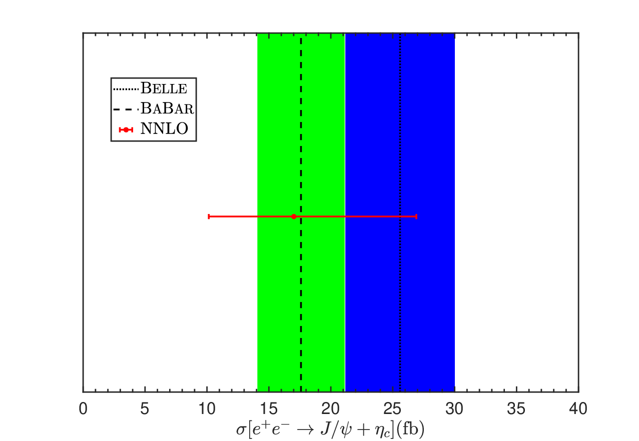
As a summary, we have calculated the NNLO QCD corrections of $J/\psi+\eta_{c}$ production in $e^{+}e^{-}$ annihilation at center-of-mass energy $\sqrt{s}=10.58$ GeV. The NNLO corrections to the total cross section for $e^{+}e^{-}\to J/\psi+\eta_{c}$ is sizable, but not comparable to the NLO corrections. It exhibits reasonable perturbative convergence behavior. More explicitly, the total cross section for $e^{+}e^{-}\to J/\psi+\eta_{c}$ is enhanced by $17\%$ in the case of $\mu_{R}=2m_{c}$ after including the NNLO corrections. From Fig. 2, we find that the $\mu_{R}$ dependence of the total cross section is reduced at the NNLO level for $\mu_{\Lambda}=m_{c}$, and the predicted cross section is sensitive to the charm quark pole mass. Combining the results shown in Table 1 and 2, we obtain the final NNLO QCD corrections to $J/\psi+\eta_{c}$ production at the $B$ factories, i.e.,

where the central value is obtained by taking $m_{c}=1.5{\rm GeV}$, $\mu_{R}=2m_{c}$ and $\mu_{\Lambda}=m_{c}$. The first uncertainty is estimated by varying $m_{c}\in[1.3,1.7]{\rm GeV}$, the second uncertainty is caused by varying $\mu_{R}\in[2m_{c},\sqrt{s}/2]$ and the third uncertainty is obtained by varying $\mu_{\Lambda}\in[1{\rm GeV},m_{c}]$. Fig. 3 shows that this prediction can both overlap with the BABAR and BELLE measurements within errors. The following work of this process is focus on improving the $\mu_{R}$ dependence.

References

- (1) H. Fritzsch, Producing Heavy Quark Flavors in Hadronic Collisions: A Test of Quantum Chromodynamics, Phys. Lett. B 67 (1977) 217–221.
- (2) F. Halzen, Cvc for Gluons and Hadroproduction of Quark Flavors, Phys. Lett. B 69 (1977) 105–108.
- (3) C.-H. Chang, Hadronic Production of Associated With a Gluon, Nucl. Phys. B 172 (1980) 425–434.
- (4) E. L. Berger and D. L. Jones, Inelastic Photoproduction of J/psi and Upsilon by Gluons, Phys. Rev. D 23 (1981) 1521–1530.
- (5) T. Matsui and H. Satz, Suppression by Quark-Gluon Plasma Formation, Phys. Lett. B 178 (1986) 416–422.
- (6) G. T. Bodwin, E. Braaten, and G. P. Lepage, Rigorous QCD analysis of inclusive annihilation and production of heavy quarkonium, Phys. Rev. D 51 (1995) 1125–1171, [hep-ph/9407339]. [Erratum: Phys.Rev.D 55, 5853 (1997)].
- (7) N. Brambilla et al., Heavy Quarkonium: Progress, Puzzles, and Opportunities, Eur. Phys. J. C 71 (2011) 1534, [arXiv:1010.5827].
- (8) A. Andronic et al., Heavy-flavour and quarkonium production in the LHC era: from proton–proton to heavy-ion collisions, Eur. Phys. J. C 76 (2016), no. 3 107, [arXiv:1506.03981].
- (9) J.-P. Lansberg, New Observables in Inclusive Production of Quarkonia, Phys. Rept. 889 (2020) 1–106, [arXiv:1903.09185].
- (10) A.-P. Chen, Y.-Q. Ma, and H. Zhang, A Short Theoretical Review of Charmonium Production, Adv. High Energy Phys. 2022 (2022) 7475923, [arXiv:2109.04028].
- (11) Belle Collaboration, K. Abe et al., Observation of double c anti-c production in e+ e- annihilation at s**(1/2) approximately 10.6-GeV, Phys. Rev. Lett. 89 (2002) 142001, [hep-ex/0205104].
- (12) Belle Collaboration, K. Abe et al., Study of double charmonium production in e+ e- annihilation at s**(1/2) ~ 10.6-GeV, Phys. Rev. D 70 (2004) 071102, [hep-ex/0407009].
- (13) BaBar Collaboration, B. Aubert et al., Measurement of double charmonium production in annihilations at GeV, Phys. Rev. D 72 (2005) 031101, [hep-ex/0506062].
- (14) E. Braaten and J. Lee, Exclusive Double Charmonium Production from Annihilation into a Virtual Photon, Phys. Rev. D 67 (2003) 054007, [hep-ph/0211085]. [Erratum: Phys.Rev.D 72, 099901 (2005)].
- (15) K.-Y. Liu, Z.-G. He, and K.-T. Chao, Problems of double charm production in e+ e- annihilation at s**(1/2) = 10.6-GeV, Phys. Lett. B 557 (2003) 45–54, [hep-ph/0211181].
- (16) K. Hagiwara, E. Kou, and C.-F. Qiao, Exclusive productions at colliders, Phys. Lett. B 570 (2003) 39–45, [hep-ph/0305102].
- (17) G. T. Bodwin, D. Kang, T. Kim, J. Lee, and C. Yu, Relativistic Corrections to e+ e- — J/psi + eta(c) in a Potential Model, AIP Conf. Proc. 892 (2007), no. 1 315–317, [hep-ph/0611002].
- (18) Z.-G. He, Y. Fan, and K.-T. Chao, Relativistic corrections to J/psi exclusive and inclusive double charm production at B factories, Phys. Rev. D 75 (2007) 074011, [hep-ph/0702239].
- (19) G. T. Bodwin, J. Lee, and C. Yu, Resummation of Relativistic Corrections to e+ e- — J/psi + eta(c), Phys. Rev. D 77 (2008) 094018, [arXiv:0710.0995].
- (20) J. P. Ma and Z. G. Si, Predictions for e+ e- — J/psi eta(c) with light-cone wave-functions, Phys. Rev. D 70 (2004) 074007, [hep-ph/0405111].
- (21) A. E. Bondar and V. L. Chernyak, Is the BELLE result for the cross section sigma(e+ e- — J / psi + eta(c)) a real difficulty for QCD?, Phys. Lett. B 612 (2005) 215–222, [hep-ph/0412335].
- (22) G. T. Bodwin, D. Kang, and J. Lee, Reconciling the light-cone and NRQCD approaches to calculating e+ e- — J/psi + eta(c), Phys. Rev. D 74 (2006) 114028, [hep-ph/0603185].
- (23) V. V. Braguta, Double charmonium production at B-factories within light cone formalism, Phys. Rev. D 79 (2009) 074018, [arXiv:0811.2640].
- (24) L. Zeng, H.-B. Fu, D.-D. Hu, L.-L. Chen, W. Cheng, and X.-G. Wu, Revisiting the production of via the annihilation within the QCD light-cone sum rules, Phys. Rev. D 103 (2021), no. 5 056012, [arXiv:2102.01842].
- (25) Y.-J. Zhang, Y.-j. Gao, and K.-T. Chao, Next-to-leading order QCD correction to e+ e- — J / psi + eta(c) at s**(1/2) = 10.6-GeV, Phys. Rev. Lett. 96 (2006) 092001, [hep-ph/0506076].
- (26) B. Gong and J.-X. Wang, QCD corrections to plus production in annihilation at = 10.6-GeV, Phys. Rev. D 77 (2008) 054028, [arXiv:0712.4220].
- (27) H.-R. Dong, F. Feng, and Y. Jia, correction to at factories, Phys. Rev. D 85 (2012) 114018, [arXiv:1204.4128].
- (28) X.-H. Li and J.-X. Wang, correction to plus production in annihilation at 10.6 GeV, Chin. Phys. C 38 (2014) 043101, [arXiv:1301.0376].
- (29) Z. Sun, X.-G. Wu, Y. Ma, and S. J. Brodsky, Exclusive production of at the factories Belle and Babar using the principle of maximum conformality, Phys. Rev. D 98 (2018), no. 9 094001, [arXiv:1807.04503].
- (30) S. J. Brodsky, M. Mojaza, and X.-G. Wu, Systematic Scale-Setting to All Orders: The Principle of Maximum Conformality and Commensurate Scale Relations, Phys. Rev. D 89 (2014) 014027, [arXiv:1304.4631].
- (31) J.-M. Shen, X.-G. Wu, B.-L. Du, and S. J. Brodsky, Novel All-Orders Single-Scale Approach to QCD Renormalization Scale-Setting, Phys. Rev. D 95 (2017), no. 9 094006, [arXiv:1701.08245].
- (32) X.-G. Wu, J.-M. Shen, B.-L. Du, X.-D. Huang, S.-Q. Wang, and S. J. Brodsky, The QCD renormalization group equation and the elimination of fixed-order scheme-and-scale ambiguities using the principle of maximum conformality, Prog. Part. Nucl. Phys. 108 (2019) 103706, [arXiv:1903.12177].
- (33) X.-D. Huang, J. Yan, H.-H. Ma, L. Di Giustino, J.-M. Shen, X.-G. Wu, and S. J. Brodsky, Detailed Comparison of Renormalization Scale-Setting Procedures based on the Principle of Maximum Conformality, arXiv:2109.12356.
- (34) F. Feng, Y. Jia, Z. Mo, W.-L. Sang, and J.-Y. Zhang, Next-to-next-to-leading-order QCD corrections to at factories, arXiv:1901.08447.
- (35) X. Liu, Y.-Q. Ma, and C.-Y. Wang, A Systematic and Efficient Method to Compute Multi-loop Master Integrals, Phys. Lett. B 779 (2018) 353–357, [arXiv:1711.09572].
- (36) X. Liu, Y.-Q. Ma, W. Tao, and P. Zhang, Calculation of Feynman loop integration and phase-space integration via auxiliary mass flow, Chin. Phys. C 45 (2021), no. 1 013115, [arXiv:2009.07987].
- (37) X. Liu and Y.-Q. Ma, Multiloop corrections for collider processes using auxiliary mass flow, Phys. Rev. D 105 (2022), no. 5 L051503, [arXiv:2107.01864].
- (38) X. Liu and Y.-Q. Ma, AMFlow: A Mathematica package for Feynman integrals computation via auxiliary mass flow, Comput. Phys. Commun. 283 (2023) 108565, [arXiv:2201.11669].
- (39) A. Czarnecki and K. Melnikov, Two loop QCD corrections to the heavy quark pair production cross-section in e+ e- annihilation near the threshold, Phys. Rev. Lett. 80 (1998) 2531–2534, [hep-ph/9712222].
- (40) M. Beneke, A. Signer, and V. A. Smirnov, Two loop correction to the leptonic decay of quarkonium, Phys. Rev. Lett. 80 (1998) 2535–2538, [hep-ph/9712302].
- (41) A. Czarnecki and K. Melnikov, Charmonium decays: J / psi — e+ e- and eta(c) — gamma gamma, Phys. Lett. B 519 (2001) 212–218, [hep-ph/0109054].
- (42) B. A. Kniehl, A. Onishchenko, J. H. Piclum, and M. Steinhauser, Two-loop matching coefficients for heavy quark currents, Phys. Lett. B 638 (2006) 209–213, [hep-ph/0604072].
- (43) A. H. Hoang and P. Ruiz-Femenia, Heavy pair production currents with general quantum numbers in dimensionally regularized NRQCD, Phys. Rev. D 74 (2006) 114016, [hep-ph/0609151].
- (44) H. S. Chung, renormalization of -wave quarkonium wavefunctions at the origin, JHEP 12 (2020) 065, [arXiv:2007.01737].
- (45) CTEQ Collaboration, R. Brock et al., Handbook of perturbative QCD: Version 1.0, Rev. Mod. Phys. 67 (1995) 157–248.
- (46) Z. Sun, Next-to-leading-order study of angular distributions in at GeV, JHEP 09 (2021) 073, [arXiv:2107.02047].
- (47) B. Gong and J.-X. Wang, Next-to-leading-order QCD corrections to e+e- – J/psi(cc) at the B factories, Phys. Rev. D 80 (2009) 054015, [arXiv:0904.1103].
- (48) T. Hahn, Generating Feynman diagrams and amplitudes with FeynArts 3, Comput. Phys. Commun. 140 (2001) 418–431, [hep-ph/0012260].
- (49) R. Mertig, M. Bohm, and A. Denner, FEYN CALC: Computer algebraic calculation of Feynman amplitudes, Comput. Phys. Commun. 64 (1991) 345–359.
- (50) V. Shtabovenko, R. Mertig, and F. Orellana, New Developments in FeynCalc 9.0, Comput. Phys. Commun. 207 (2016) 432–444, [arXiv:1601.01167].
- (51) J. Klappert, F. Lange, P. Maierhöfer, and J. Usovitsch, Integral reduction with Kira 2.0 and finite field methods, Comput. Phys. Commun. 266 (2021) 108024, [arXiv:2008.06494].
- (52) M. Krämer, QCD corrections to inelastic J / psi photoproduction, Nucl. Phys. B 459 (1996) 3–50, [hep-ph/9508409].
- (53) D. J. Broadhurst, N. Gray, and K. Schilcher, Gauge invariant on-shell Z(2) in QED, QCD and the effective field theory of a static quark, Z. Phys. C 52 (1991) 111–122.
- (54) S. Bekavac, A. Grozin, D. Seidel, and M. Steinhauser, Light quark mass effects in the on-shell renormalization constants, JHEP 10 (2007) 006, [arXiv:0708.1729].
- (55) M. Czakon, A. Mitov, and S. Moch, Heavy-quark production in massless quark scattering at two loops in QCD, Phys. Lett. B 651 (2007) 147–159, [arXiv:0705.1975].
- (56) M. Czakon, A. Mitov, and S. Moch, Heavy-quark production in gluon fusion at two loops in QCD, Nucl. Phys. B 798 (2008) 210–250, [arXiv:0707.4139].
- (57) M. Fael, K. Schönwald, and M. Steinhauser, Exact results for and with two mass scales and up to three loops, JHEP 10 (2020) 087, [arXiv:2008.01102].
- (58) P. Bärnreuther, M. Czakon, and P. Fiedler, Virtual amplitudes and threshold behaviour of hadronic top-quark pair-production cross sections, JHEP 02 (2014) 078, [arXiv:1312.6279].
- (59) W. Tao, R. Zhu, and Z.-J. Xiao, Next-to-next-to-leading order matching of beauty-charmed meson and decay constants, arXiv:2209.15521.
- (60) Particle Data Group Collaboration, R. L. Workman et al., Review of Particle Physics, PTEP 2022 (2022) 083C01.
- (61) F. Herren and M. Steinhauser, Version 3 of RunDec and CRunDec, Comput. Phys. Commun. 224 (2018) 333–345, [arXiv:1703.03751].
- (62) H.-M. Yu, W.-L. Sang, X.-D. Huang, J. Zeng, X.-G. Wu, and S. J. Brodsky, Scale-fixed predictions for production in electron-positron collisions at NNLO in perturbative QCD, JHEP 01 (2021) 131, [arXiv:2007.14553].