AsyInst: Asymmetric Affinity with DepthGrad and Color for Box-Supervised Instance Segmentation
Abstract
The weakly supervised instance segmentation is a challenging task. The existing methods typically use bounding boxes as supervision and optimize the network with a regularization loss term such as pairwise color affinity loss for instance segmentation. Through systematic analysis, we found that the commonly used pairwise affinity loss has two limitations: (1) it works with color affinity but leads to inferior performance with other modalities such as depth gradient, (2)the original affinity loss does not prevent trivial predictions as intended but actually accelerates this process due to the affinity loss term being symmetric. To overcome these two limitations, in this paper, we propose a novel asymmetric affinity loss which provides the penalty against the trivial prediction and generalizes well with affinity loss from different modalities. With the proposed asymmetric affinity loss, our method outperforms the state-of-the-art methods on the Cityscapes dataset and outperforms our baseline method by 3.5% in mask AP.
1 Introduction
Instance segmentation is an important yet challenging task in computer vision he2017mask; huang2019mask; chen2020blendmask; cheng2020boundary; wang2020solo; tian2020conditional; wang2020solov2; li2017fully; liu2018path; chen2019hybrid; de2017semantic; newell2017associative; liu2017sgn; gao2019ssap; bolya2019yolact. It requires models to predict the localization of the object and to predict the fine-grained segmentation masks of objects. The training of instance segmentation models requires fine-grained pixel-wised annotations which are expensive and time-consuming to obtain.
To avoid annotating large-scale fine-grained pixel-wised datasets, recently, there are a few attempts to train the model with bounding box labels Khoreva_2017_CVPR; NEURIPS2019_e6e71329; tian2021boxinst; li2022box; lan2021discobox. By training with box-level labels, the cost of training data collection can be greatly reduced. Normally, these methods supervise the model training by using the pairwise loss based on different kinds of inductive prior from images including color similarity tian2021boxinst or bounding box tightness NEURIPS2019_e6e71329. Among all the work, BoxInst tian2021boxinst proposed to use pairwise color affinity loss to optimize the model and achieved promising results. The proposed pairwise color affinity loss enables the model to be learned with pixel-wised fine-level supervision based on the prior knowledge of the color information. Furthermore, this pairwise affinity loss doesn’t necessarily depend on color similarity alone and should be capable to be generalized to other modalities as well.
As the existing work mainly relies on RGB images for box-supervised instance segmentation, other modalities are less explored for this task. For example, depth images have a natural advantage in identifying the boundary of objects compared to color information. Therefore, an intuitive idea would be applying the pairwise affinity loss with depth gradient affinity under a simple observation that depth gradient tends to be more consistent in the non-boundary area of objects but only encounters performance drop in mask accuracy. However, we observed that simply adopting the affinity loss on the depth gradient would lead to inferior performance. And our study shows that the original affinity loss being symmetric is the reason behind low performance which not only makes the pairwise affinity loss incompatible with other modalities such as depth gradient but also hurt performance with color affinity.
To understand the limitation of the affinity loss, we visualized the optimization surface of the loss in 3D space in Fig. 4. The saddle-shaped landscape of symmetric affinity loss consists of two halves one of which converges to produce double-negative pixel pairs whereas the other one converges to produce double-positive pixel pairs In addition to the symmetry, the double-positive half of the affinity loss is more effective than the other one under the influence of non-positive gradient from the projection loss tian2021boxinst, which is a widely used method to provide box-level supervision tian2021boxinst; li2022box. This behavior results in trivial predictions such as box-shaped masks. More details related to the interaction between symmetric affinity loss and projection loss can be found in Section 4.
Therefore, we intend to propose an asymmetric affinity loss to increase the chance of a pixel pair falling on the affinity loss’s double-negative half to compensate for the bias towards positive pixels from the projection loss. More specifically, we add an offset into the original symmetric affinity loss which controls the degree of asymmetry of the affinity loss. Although a large increases the asymmetry level, it also causes gradient vanishing, thus leading to slow convergence towards double-negative pixel pairs, which decreases the desired compensating bias. A smoothness hyper-parameter is then introduced to reshape the loss function and alleviate gradient vanishing. Some qualitative results shown in demonstrate that the original symmetric affinity loss worsens convergence to trivial box-shaped predictions while our proposed asymmetric affinity loss prevents it.
The proposed asymmetric affinity loss not only works well with depth-grad affinity but also improves the previously proposed symmetric affinity loss with color affinity, demonstrating that the proposed asymmetric affinity loss can be a general form of pairwise regularization with both color and depth-grad affinity while the symmetric one can only work with color affinity.
To summarise, the main contribution of this paper is threefold:
- •
We propose a novel approach to improve the box-supervised instance segmentation model with depth information via depth gradient affinity.
- •
Through extensive analysis, we reveal a previously overlooked common flaw in symmetric affinity loss and propose a simple yet effective solution to address it by making it asymmetric.
- •
We conduct thorough and conclusive experiments showing the effectiveness of the proposed asymmetric affinity loss. And the proposed AsyInst with both color and depth affinity achieves a total performance improvement of 3.54% compared to our baseline on Cityscapes Cordts2016Cityscapes.
2 Related Work
Instance Segmentation:
is a challenging task requiring both instance-level and pixel-level predictions and has attracted increasing attention. The existing work can be classified into three categories. The top-down methods li2017fully; he2017mask; liu2018path; chen2019hybrid tackle instance segmentation by detecting objects first and then predicting masks inside the detected bounding box. The bottom-up methods de2017semantic; newell2017associative; liu2017sgn; gao2019ssap adopt a classify-then-cluster paradigm in which semantic segmentation is first performed on an image before pixels are clustered into objects with pixel-wise embeddings. Some recent methods bolya2019yolact; tian2020conditional; chen2020blendmask; wang2020solo; wang2020solov2 follow a hybrid pattern by combining both top-down and bottom-up approaches which achieve high performance with a computational cost comparable to detection models. Although performing pixel-level predictions in addition to instance-level predictions with little computation overhead, instance segmentation models are still not used as widely as object detection models in the industry mainly due to the highly expensive mask annotations, demonstrating the urgency and importance of box-supervised instance segmentation methods.
Box-supervised Instance Segmentation:
The Box-supervised instance segmentation with deep learning has been less explored so far. SDI Khoreva_2017_CVPR is the first instance segmentation model with deep learning and uses GrabCut to generate pseudo segmentation ground-truth providing pixel-wise supervision. BBTP NEURIPS2019_e6e71329 formulates the box-supervised instance segmentation as a multiple instance learning problem where the positive and negative bags are sampled according to box annotations on which unary loss is applied. BBTP also utilizes pairwise affinity loss but both the unary loss and pairwise affinity loss are defined only based on box annotation and there is no supervision for segmentation finer than box annotation. BoxInst tian2021boxinst proposes to use projection loss and color affinity loss to supervise segmentation prediction on the box level and pixel-pair level respectively. Despite the proposed color affinity loss appearing to be very effective, its performance is sub-optimal and can be further improved due to its symmetry based on our analysis and experiment results. None of the above mentioned methods use depth information alone with box annotations, which have a natural advantage at identifying objects’ boundaries and is cheap to acquire in contrast to actual fine-grained mask annotations.
3 Depth-Grad Affinity Regularization
In this section, we give a formal definition of the depth gradient affinity and a detailed design of a pairwise affinity loss based on this depth gradient affinity.
3.1 Definition of Depth Gradient Affinity

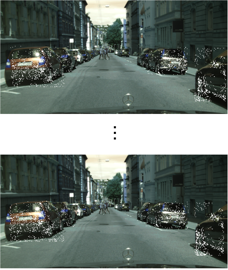
Naturally, depth maps contain more information about objects’ shapes and boundaries. As shown in Fig. 1, it can be observed that depth gradient (depth-grad) values are more consistent near non-boundary areas. Thus, it is intuitive to assume the pixels with similar depth-grad should have the same pixel-wise mask label and vice versa.
However, such an assumption isn’t always applicable in the real world. Pixels on the uneven surface of objects may have different gradient values but still share the same pixel label. For example, as shown in Fig. 1, pixels around the cube’s edge located inside the green bounding box are less consistent. In other words, the label relationship between pixels which doesn’t share similar depth gradient can be agnostic. Therefore, we only consider the pixels with similar depth gradient values in the definition of depth gradient affinity.
Considering an arbitrary pixel in the image connected with first-order neighbours while each has a corresponding second-order neighbour as shown in Fig. 2(a), the depth gradient between and is denoted as while where are respectively the depth values of . Then an edge connecting and is determined as a positive edge in which and have the same label when the difference between and is smaller than a threshold , i.e.
| (1) |
where is the gradient difference of the edge and is the threshold for gradient difference
3.2 Depth-Grad Affinity Loss
Similar to the color affinity loss of BoxInst tian2021boxinst, we only consider the situation that in which the edge’s label should be since the can be agnostic when due to the reasons discussed in Section 3.1.
As being a positive edge implies that and linked by have the same label, the probability of is
| (2) |
where the and are the logits of pixels and , and the sigmoid function meaning that and are the probability of and being the foreground pixel while and are the probability of and being the negative pixel.
Thus, the depth-grad affinity loss is defined as
| (3) |
where is the set of edges where the corresponding all have a valid depth value and at least one end in the bounding box, and is the number of edges in which also satisfy . The purpose of only using edges in is to focus the regularization inside the box since projection loss can already provide sufficient regularization outside the box.
4 Coupling between Projection Loss and Symmetric Affinity loss
The proposed depth gradient affinity loss is very reasonably defined based on the experience of color affinity loss proposed in BoxInst tian2021boxinst. However, naively adopting this fashion of pairwise affinity loss with depth gradient affinity has a negative impact on model performance. As illustrated in , the models trained with depth gradient affinity loss tend to produce trivial box-shaped masks. This is due to that the symmetric property of pairwise affinity loss leads to harmful coupling interaction between the projection loss tian2021boxinst and the pairwise affinity loss.
4.1 Preference of towards False Positive Pixels
The projection loss, originally proposed by Boxinst tian2021boxinst, requires the projection of a predicted probability score mask to be aligned with the corresponding bounding box horizontally and vertically. The horizontal and vertical projection of are acquired with a max operation along each axis, i.e.
| (4) |
where are the horizontal and vertical projection of respectively.
Similarly, we can obtain the horizontal and vertical projection of a bounding box noted as , which will be used as ground-truth for . Thus, the projection loss tian2021boxinst is defined as
| (5) |
where is the Dice loss defined as
| (6) |
Considering the horizontal term of the projection loss in Eq. 5, the gradient of to is
| (7) |
For a pixel in the horizontal projection with the probability score and the corresponding ground-truth score , the if the pixel is horizontal inside the bounding box and if otherwise.
The gradient of to is
| (8) |
The horizontal projection of the predicted mask is acquired through max operation based on Eq. 4 meaning that all the elements in the gradient are non-negative. We can infer that the gradient of to any probability scores from the in-box part of is non-positive while vice versa for probability scores from the out-box part of .

As a similar conclusion applies for the gradient of the vertical term in Eq. 5, the pixels inside the box can only receive a non-positive gradient from the projection loss which tends to increase the probability scores while vice versa for the pixels outside the box. Thus, the projection loss encourages false positives inside the box leading to trivial predictions such as box-shaped masks as shown in Fig. 3.
4.2 Problem with Symmetric Affinity Loss
BoxInst tian2021boxinst introduces color affinity loss to provide finer supervision in compensation for the coarse supervision from the projection loss which encourages the model to produce false positive pixels leading to trivial predictions such as bbox-shaped masks, but it does little to alleviate this problem if not worsen it. As shown in the Fig. 4, symmetric affinity loss encourages pixel pairs linked by edges to be double-positive pairs as well as double-negative pairs. However, under the influence of non-positive gradient from the projection loss which constantly tends to increase the probability score , it is far more likely for a pixel pair to land on the double-positive half of the affinity loss than the double-negative one, accelerating the process to produce trivial solutions.
This results in a significant performance drop when naively adopting depth-grad affinity regularization in the form of Eq. 3. Although color affinity loss proposed in Boxinst improve the performance by a stable and substantial margin, it shares this flaw leading to its current sub-optimal performance. More analysis about this will be discussed in Sections 6.2 and 6.3.
5 Asymmetric Pairwise Affinity Loss
Since this harmful coupling process which leads to trivial predictions is due to the affinity loss being symmetric, we intend to tackle this optimization problem by adjusting the landscape of affinity loss thus introducing asymmetry, which can provide a penalty against trivial predictions. We hence introduce our simple yet effective solution.
5.1 Introducing Asymmetry with
An intuitive solution to address this flaw of the affinity loss is by making it asymmetric therefore increasing the chance of pixel pairs falling on the double-negative half to compensate for the existing bias from the projection loss towards positive predictions. We hence make a simple modification to the original affinity loss by adding an offset to the Eq. 2, i.e.
| (9) |
.
As shown in Fig. 5(a), pairwise affinity loss with a positive is more likely to converge at compared to hence reduce the model’s tendency to produce trivial predictions.
5.2 Gradient Vanishing with Large
While introducing a strong bias, large results in a large plain area in the landscape of affinity loss causing gradient vanishing and slow convergence which undermine the purpose of using asymmetric affinity loss to introduce a bias towards negative predictions. We therefore propose to increase the gradient at a lower loss value by adding a modulating factor with a smoothness parameter to the Eq. 3. We then define the final formula of asymmetric depth-grad affinity loss as
| (10) |
As illustrated in Fig. 5(b), the proposed modulating factor in Eq. 10 greatly helps to alleviate the gradient vanishing issue caused by large .

5.3 Overall Learning Objective
The affinity loss functions for color and depth are defined in a similar fashion, therefore, we can propose a general form of asymmetric affinity loss as:
| (11) |
Then the color affinity and depth affinity can be formulated as
| (12) |
where is the set of edges that at least has one pixel inside the box, and is color similarity threshold.
The overall learning objective for prediction in our AsyInst is defined as
| (13) |
where and as the respective loss weight for color and depth affinity loss which are linearly warmed up during the early iterations to stabilize the training.
| Method | col. affinity | dep. affinity | AP | ||
| Sym. | Asy. | Sym. | Asy. | ||
| w/o color affinity: | |||||
| Baseline | 18.596 | ||||
| AsyInst | 15.413 | ||||
| AsyInst | 19.547 | ||||
| w/ color affinity: | |||||
| Baseline | 21.145 | ||||
| AsyInst | 19.948 | ||||
| AsyInst | 21.669 | ||||
| AsyInst | 24.687 | ||||
| Method | AP | AP50 | person | rider | car | truck | bus | train | motor-cycle | bicycle |
|---|---|---|---|---|---|---|---|---|---|---|
| BoxInst tian2021boxinst | 21.15 | 49.50 | 20.30 | 5.84 | 37.17 | 23.16 | 43.63 | 21.19 | 10.87 | 7.04 |
| BoxLevelSet li2022box | 17.9 | 38.0 | 11.4 | 6.01 | 28.14 | 20.76 | 38.72 | 24.09 | 7.67 | 6.33 |
| AsyInst (w/o depth) | 24.10 | 52.27 | 23.29 | 9.33 | 39.32 | 26.57 | 43.47 | 27.14 | 13.60 | 9.37 |
| AsyInst | 24.69 | 53.01 | 22.91 | 9.89 | 39.24 | 26.38 | 46.62 | 31.89 | 12.52 | 8.05 |
6 Experiments
We conduct ablation studies about detailed designs in our model AsyInst and compare AsyInst’s performance with other state-of-the-art box-supervised instance segmentation methods on Cityscapes Cordts2016Cityscapes.
6.1 Experimental Settings
Dataset.
We evaluate our method on Cityscapes Cordts2016Cityscapes. Disparity maps from Cityscapes are converted to depth maps according to official instructions11 1 https://github.com/mcordts/cityscapesScripts/blob/master/README.md. Ablation studies are trained on Cityscapes training set and evaluated on Cityscapes validation set by default.
Model.
We use ResNet-50 he2016deep with FPN lin2017feature as the backbone in all the experiments. The first stage of ResNet-50 and all the batchnorm layers are frozen following the default setting in Detectron2 wu2019detectron2. We use BoxInst tian2021boxinst as the baseline model with or without symmetric color affinity loss. The depth gradient threshold is 0.01. , , , are respectively 2.5, 1.5, 3.5, 2.5. Loss weights and are set as 1.0 and 0.1 respectively, which are linearly warmed up during the first 10k iterations. All the remaining hyper-parameters regarding affinity loss including color similarity threshold and dilation size are the same as ones in BoxInst unless specified.
Training Details.
Experiments on Cityscapes follow the training details in Detectron2wu2019detectron2 that models are trained with a total batch size of 8 on 8 GPUs (i.e. NVIDIA RTX Titan) for 24k iterations using SGD optimizer with base learning rate set as 0.01 and reduced to 0.001 at iteration 18k. Weight decay and momentum for both datasets are set as 1e-4 and 0.9 respectively. Random flipping and scaling are applied sequentially for experiments on both Cityscapes. Due to the high resolution of images on Cityscapes, images are first randomly cropped to half size (512 * 1024) during training. No augmentation is applied during inference. Same as CondInst tian2020conditional which is the fully-supervised model our AsyInst is based on, the stride of output segmentation masks is set to 2. BoxLevelSet li2022box in Table 2 is a re-implementation based on the offical code 22 2 https://github.com/LiWentomng/boxlevelset which does not support the Cityscapes dataset. To adapt to it, with some hyper parameter tuning, we set the learning rate as 1e-4.
| Sym. | ||||
|---|---|---|---|---|
| col. affinity: | 21.145 | / | / | / |
| / | 22.868 | 23.144 | 17.927 | |
| / | 23.821 | 24.095 | 23.410 | |
| / | 24.076 | 24.062 | 23.933 | |
| dep. affinity: | 15.413 | / | / | / |
| / | 18.127 | 18.308 | 18.653 | |
| / | 18.505 | 18.861 | 19.465 | |
| / | 18.379 | 19.069 | 19.547 | |
6.2 Performance Improvement from Asymmetry
Here we study how the introduced asymmetry in the affinity loss can reverse the negative impact of symmetric affinity loss with depth gradient affinity. We trained two sets of baseline models and AsyInst with and without color affinity loss.
As shown in Table 1, naively adopting symmetric affinity loss with depth gradient hurts performance regardless of whether color affinity is applied. However, the performance is improved in both cases after changing the depth gradient affinity loss from being symmetric to being asymmetric. We further discover that the performance of color affinity loss can still be improved by 3.018% in mask AP when made asymmetric, proving that although the symmetric color affinity loss improves performance, it is sill sub-optimal due to its symmetry. These results indicate that our proposed asymmetric affinity loss can be used as a general form of affinity loss while the original symmetric affinity loss is only compatible with color affinity.
6.3 Asymmetry Preventing Trivial Prediction
As discussed in Sections 4 and 5, the original symmetric affinity loss accelerates convergence to trivial predictions while the asymmetric affinity in our AsyInst prevents this. Here we study the effect of asymmetric affinity loss preventing trivial prediction with qualitative results on Cityscapes. To enhance the visual effect, we also conducted experiments with increased loss weight for color or depth gradient affinity loss to the 5 times of the original setting described in Section 5.3, i.e. . To study the color and depth gradient affinity individually, color and depth gradient affinity loss are not utilized simultaneously during training in this ablation study.
The qualitative results shown in Fig. 6 demonstrate that asymmetry is the key to affinity loss to prevent trivial predictions, especially when utilized with depth gradient affinity. Mask predictions from models trained with symmetric affinity loss are usually squarer and fill more blank space inside boxes compared to models trained with asymmetric affinity.
6.4 Effect of and
We introduce the in Section 5.1 and in Section 5.2 to control the affinity loss’s asymmetry degree and gradient vanishing respectively. To examine whether these two hyper-parameters work as intended, we conduct the following ablation studies.
Performance of AsyInst trained with different combinations of and are shown in Table 3. For better comparison, we only use color affinity or depth gradient affinity for each experiment in this ablation study. As shown in Fig. 7, performance tends to get improved with larger which enhances asymmetry and introduces stronger penalties against trivial predictions. However, extremely large could hurt performance due to gradient vanishing as discussed in Section 5.2 while increasing mitigates this performance drop.
6.5 Comparison with State-of-the-art
We compare AsyInst with state-of-the-art box-supervised instance segmentation methods on Cityscapes Cordts2016Cityscapes. As shown in Table 2, AsyInst outperforms all the previous methods by a noticeable margin with or without depth information, demonstrating the superiority of the proposed methods. AsyInst without depth affinity still surpasses the BoxInst tian2021boxinst which is also our baseline model, by 3.09% in mask AP. With additional depth information, AsyInst outperforms BoxInst by a significant margin of 3.54% in mask AP. It should also be noted that the BoxLevelSet is based on a stronger fully-supervised model that is SOLOv2 wang2020solov2 while AsyInst is based on CondInst tian2020conditional.
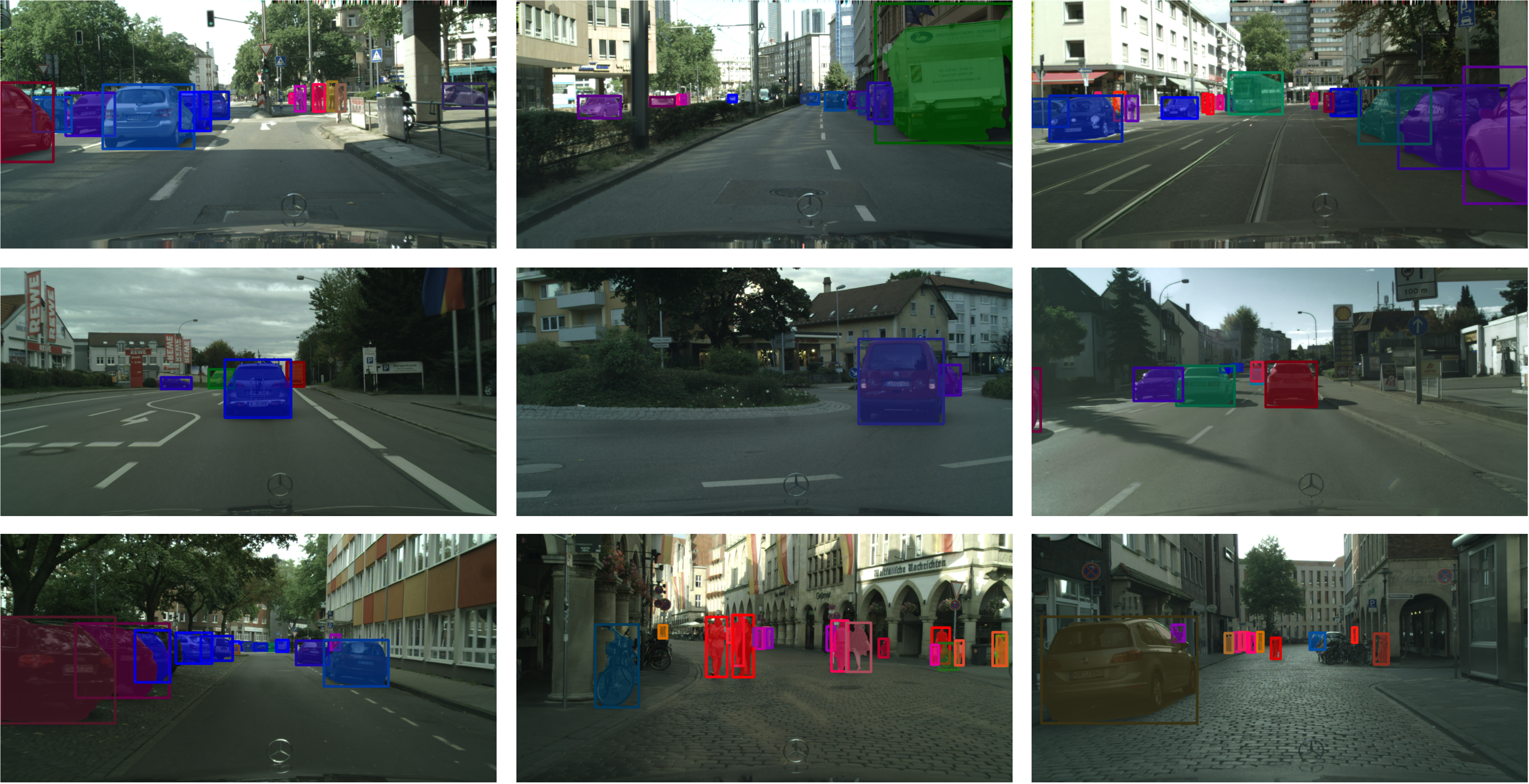
Some qualitative results from our AsyInst with the highest performance on Cityscapes validation set are illustrated in Fig. 8.
7 Conclusion
In this work, we reveal that the coupling interaction during the optimization between the projection loss and the affinity loss can lead to trivial box-shaped mask predictions when affinity loss is symmetric. This flaw of symmetry has a negative impact on the performance of affinity loss and makes it totally incompatible with other potentially helpful modalities such as depth gradients. Our proposed asymmetric affinity loss tackles this issue and can act as a general form of affinity loss with both color and depth gradient affinity. We believe this work can inspire future exploration into pairwise affinity regularization with various modalities.
References
- (1) Daniel Bolya, Chong Zhou, Fanyi Xiao, and Yong Jae Lee. Yolact: Real-time instance segmentation. In Proceedings of the IEEE/CVF international conference on computer vision, pages 9157–9166, 2019.
- (2) Hao Chen, Kunyang Sun, Zhi Tian, Chunhua Shen, Yongming Huang, and Youliang Yan. Blendmask: Top-down meets bottom-up for instance segmentation. In Proceedings of the IEEE/CVF conference on computer vision and pattern recognition, pages 8573–8581, 2020.
- (3) Kai Chen, Jiangmiao Pang, Jiaqi Wang, Yu Xiong, Xiaoxiao Li, Shuyang Sun, Wansen Feng, Ziwei Liu, Jianping Shi, Wanli Ouyang, et al. Hybrid task cascade for instance segmentation. In Proceedings of the IEEE/CVF Conference on Computer Vision and Pattern Recognition, pages 4974–4983, 2019.
- (4) Tianheng Cheng, Xinggang Wang, Lichao Huang, and Wenyu Liu. Boundary-preserving mask r-cnn. In European conference on computer vision, pages 660–676. Springer, 2020.
- (5) Marius Cordts, Mohamed Omran, Sebastian Ramos, Timo Rehfeld, Markus Enzweiler, Rodrigo Benenson, Uwe Franke, Stefan Roth, and Bernt Schiele. The cityscapes dataset for semantic urban scene understanding. In Proc. of the IEEE Conference on Computer Vision and Pattern Recognition (CVPR), 2016.
- (6) Bert De Brabandere, Davy Neven, and Luc Van Gool. Semantic instance segmentation with a discriminative loss function. arXiv preprint arXiv:1708.02551, 2017.
- (7) Naiyu Gao, Yanhu Shan, Yupei Wang, Xin Zhao, Yinan Yu, Ming Yang, and Kaiqi Huang. Ssap: Single-shot instance segmentation with affinity pyramid. In Proceedings of the IEEE/CVF International Conference on Computer Vision, pages 642–651, 2019.
- (8) Kaiming He, Georgia Gkioxari, Piotr Dollár, and Ross Girshick. Mask r-cnn. In Proceedings of the IEEE international conference on computer vision, pages 2961–2969, 2017.
- (9) Kaiming He, Xiangyu Zhang, Shaoqing Ren, and Jian Sun. Deep residual learning for image recognition. In Proceedings of the IEEE conference on computer vision and pattern recognition, pages 770–778, 2016.
- (10) Cheng-Chun Hsu, Kuang-Jui Hsu, Chung-Chi Tsai, Yen-Yu Lin, and Yung-Yu Chuang. Weakly supervised instance segmentation using the bounding box tightness prior. In H. Wallach, H. Larochelle, A. Beygelzimer, F. d'Alché-Buc, E. Fox, and R. Garnett, editors, Advances in Neural Information Processing Systems, volume 32. Curran Associates, Inc., 2019.
- (11) Zhaojin Huang, Lichao Huang, Yongchao Gong, Chang Huang, and Xinggang Wang. Mask scoring r-cnn. In Proceedings of the IEEE/CVF conference on computer vision and pattern recognition, pages 6409–6418, 2019.
- (12) Anna Khoreva, Rodrigo Benenson, Jan Hosang, Matthias Hein, and Bernt Schiele. Simple does it: Weakly supervised instance and semantic segmentation. In Proceedings of the IEEE Conference on Computer Vision and Pattern Recognition (CVPR), July 2017.
- (13) Shiyi Lan, Zhiding Yu, Christopher Choy, Subhashree Radhakrishnan, Guilin Liu, Yuke Zhu, Larry S Davis, and Anima Anandkumar. Discobox: Weakly supervised instance segmentation and semantic correspondence from box supervision. In Proceedings of the IEEE/CVF International Conference on Computer Vision, pages 3406–3416, 2021.
- (14) Wentong Li, Wenyu Liu, Jianke Zhu, Miaomiao Cui, Xian-Sheng Hua, and Lei Zhang. Box-supervised instance segmentation with level set evolution. In European Conference on Computer Vision, pages 1–18. Springer, 2022.
- (15) Yi Li, Haozhi Qi, Jifeng Dai, Xiangyang Ji, and Yichen Wei. Fully convolutional instance-aware semantic segmentation. In Proceedings of the IEEE conference on computer vision and pattern recognition, pages 2359–2367, 2017.
- (16) Tsung-Yi Lin, Piotr Dollár, Ross Girshick, Kaiming He, Bharath Hariharan, and Serge Belongie. Feature pyramid networks for object detection. In Proceedings of the IEEE conference on computer vision and pattern recognition, pages 2117–2125, 2017.
- (17) Shu Liu, Jiaya Jia, Sanja Fidler, and Raquel Urtasun. Sgn: Sequential grouping networks for instance segmentation. In Proceedings of the IEEE International Conference on Computer Vision, pages 3496–3504, 2017.
- (18) Shu Liu, Lu Qi, Haifang Qin, Jianping Shi, and Jiaya Jia. Path aggregation network for instance segmentation. In Proceedings of the IEEE conference on computer vision and pattern recognition, pages 8759–8768, 2018.
- (19) Alejandro Newell, Zhiao Huang, and Jia Deng. Associative embedding: End-to-end learning for joint detection and grouping. Advances in neural information processing systems, 30, 2017.
- (20) Zhi Tian, Chunhua Shen, and Hao Chen. Conditional convolutions for instance segmentation. In European conference on computer vision, pages 282–298. Springer, 2020.
- (21) Zhi Tian, Chunhua Shen, Xinlong Wang, and Hao Chen. Boxinst: High-performance instance segmentation with box annotations. In Proceedings of the IEEE/CVF Conference on Computer Vision and Pattern Recognition, pages 5443–5452, 2021.
- (22) Xinlong Wang, Tao Kong, Chunhua Shen, Yuning Jiang, and Lei Li. Solo: Segmenting objects by locations. In European Conference on Computer Vision, pages 649–665. Springer, 2020.
- (23) Xinlong Wang, Rufeng Zhang, Tao Kong, Lei Li, and Chunhua Shen. Solov2: Dynamic and fast instance segmentation. Advances in Neural information processing systems, 33:17721–17732, 2020.
- (24) Syed Waqas Zamir, Aditya Arora, Akshita Gupta, Salman Khan, Guolei Sun, Fahad Shahbaz Khan, Fan Zhu, Ling Shao, Gui-Song Xia, and Xiang Bai. isaid: A large-scale dataset for instance segmentation in aerial images. In Proceedings of the IEEE Conference on Computer Vision and Pattern Recognition Workshops, pages 28–37, 2019.
- (25) Yuxin Wu, Alexander Kirillov, Francisco Massa, Wan-Yen Lo, and Ross Girshick. Detectron2. https://github.com/facebookresearch/detectron2, 2019.
AsyInst: Asymmetric Affinity with DepthGrad and Color for Box-Supervised Instance
Appendix
Appendix A The upper limit for
As illustrated in Fig. 9 and Fig. 10, a () too large can increase the number of local maxima and make the previous maxima location another local minima, therefore there should be an upper limit for , i.e. .
A.1 Notations
Let . Similarly, we have . Specifically when , we define . Also let . Then we have
| (14) |
The gradient of sigmoid function is
| (15) |

A.2 Proof
The affinity loss having only one maxima means that there is only one solution for and .
Considering , we have
| (16) |
where
| (17) |
Similarly, we have
| (18) |
Obviously, one solution of
| (19) |
is , i.e. .
Since the Eq. 19 should have only one solution, , which is equivalent to according to Eq. 17, should have only one solution which is , or no solution at all. when .
Let . Then must be always positive, or . is at minima when , i.e.
| (20) |
Suppose , then , which contradicts with according to Eq. 20.
Suppose is always positive, then , then we have .
To Summarize,
| (21) |
Appendix B Experiments on iSAID
The iSAID waqas2019isaid is a high-resolution remote sensing dataset with annotations for instance segmentation, featuring a large number of small objects with complex backgrounds.
We train AsyInst and BoxInst tian2021boxinst, which is also our baseline, on iSAID for 12 epochs with only random horizontal flip as augmentation following BoxLevelSet li2022box. The learning rate is reduced by a scale factor of 0.1 at the 9-th and 11-th epoch. The number of proposals per image is restricted to 512 during training to reduce memory consumption. Other settings are the same as the ones used for experiments on Cityscapes Cordts2016Cityscapes.
| Method | backbone | mAP |
|---|---|---|
| BoxInst | ResNet-50-FPN | 19.2 |
| BoxLevelSet | ResNet-50-FPN | 20.1 |
| AsyInst | ResNet-50-FPN | 20.2 |
B.1 Comparison with State-of-the-art on iSAID
As shown in Table 4, AsyInst achieves highest performance on iSAID compared to former SOTA BoxLevelSet li2022box while BoxLevelSet is built based on a stronger fully-supervised model that is SOLOv2 wang2020solov2. Some qualitative results are shown in Fig. 11.
B.2 Ablation study about and on iSAID
We also conducted a ablation study about the effect of and on iSAID. Since iSAID doesn’t provide depth maps, we only study and ’s effect on color affinity here.
| Sym. | |||||
|---|---|---|---|---|---|
| col. affinity: | 19.2 | / | / | / | / |
| / | 19.5 | 19.8 | 19.3 | 14.9 | |
| / | 19.7 | 20.2 | 20.0 | 19.2 |
As shown in Table 5, these results is very similar to ones in Tab. 3 as discussed in Sec. 6.4. It can be observed that asymmetry improves the performance of color affinity loss but extremely large may hurt performance. Increasing may help mitigating this performance drop.