On Spectral Bias Reduction of Multi-scale Neural Networks for Regression Problems Thanks: October 16, 2023, submitted to SIAM J. Numerical Analysis
Abstract
In this paper, we derive diffusion equation models in the spectral domain for the evolution of training errors of two-layer multi-scale deep neural networks (MscaleDNN) [6, 30], designed to reduce the spectral bias of fully connected deep neural networks in approximating oscillatory functions. The diffusion models are obtained from the spectral form of the error equation of the MscaleDNN, derived with a neural tangent kernel approach and gradient descent training and a sine activation function, assuming a vanishing learning rate and infinite network width and domain size. The involved diffusion coefficients are shown to have larger supports if more scales are used in the MscaleDNN, and thus, the proposed diffusion equation models in the frequency domain explain the MscaleDNN’s spectral bias reduction capability. Numerical results of the diffusion models for a two-layer MscaleDNN training match with the error evolution of actual gradient descent training with a reasonably large network width, thus validating the effectiveness of the diffusion models. Meanwhile, the numerical results for MscaleDNN show error decay over a wide frequency range and confirm the advantage of using the MscaleDNN in approximating functions with a wide range of frequencies.
keywords
multi-scale deep neural network, spectral bias, diffusion equation, gradient descent method.AMS
35Q68, 65N35, 65T99,65K101 Introduction
Deep learning algorithms have achieved great success in computer vision [20, 42, 44], natural language processing [53, 35, 22] and many other areas. Their computational power with the help of graphics processing units (GPUs) and capability of handling high dimensional problems have led the computational community to investigate their potentials in applied mathematics research. As a result, a new research field known as scientific machine learning has became active in the past few years.
One important task in scientific machine learning is to use deep neural networks (DNNs) to approximate functions or solutions of partial differential equations (PDEs). The idea of using neural networks to solve PDEs goes back to the 1990’s [9, 21]. In general, four categories of deep PDE solvers have been investigated. The first category is to use deep neural networks to improve classical numerical methods [14, 17, 46]. In the second category, the solution operators between infinite-dimensional spaces are approximated by neural networks [1, 27, 26]. In the third category, the deep neural networks are utilized to approximate the solutions of PDEs directly such as the physics-informed neural networks (PINNs) [29, 38, 39], the deep Ritz method [11, 34, 28, 18], and Garkerkin methods with weak adversarial networks (WAN) [54, 7]. Lastly, Feynman-Kac formula approaches utilize the connection between linear and nonlinear PDEs and (backward) stochastic differential equations to construct loss functions for the learning algorithms [10, 16, 15, 3, 56, 4].
Despite their many successes for a wide range of applications, recent studies on the convergence of the deep learning algorithms in theories and practical computations show that standard fully connected DNNs have difficulties in learning high frequency functions, a phenomenon referred as ”spectral bias” [37] or ”F-Principle” [51, 52] in the literature. To overcome this bias, several strategies have been introduced to design neural networks with better frequency resolution, producing promising results. For solving PDEs, a multi-scale DNN (MscaleDNN) [6, 30, 47, 31, 25, 55], which consists of a series of parallel fully connected sub-neural networks receiving scaled inputs, has been proposed to learn highly oscillating solutions. Each individual scaled sub-network in the MscaleDNN is designed to approximate a segment of frequency content of the target function, and the effect of the scaling is to convert a specific range of high frequency content to a lower one so that the learning can be accomplished much faster. It was also proposed in [6, 30] that the MscaleDNN should use activation functions with a localized frequency profile, such as the sine function and compact supported functions (hat functions and B-splines, etc). In a related work for image and 3D shape reconstruction, the Fourier feature networks, which in fact can be obtained from the MscaleDNN with a sine activation function in their first layer, use the sinusoidal mapping on their inputs and dramatically improve the performance of learning [33, 57, 43].
To analyze the convergence of deep learning algorithms, the neural tangent kernel (NTK), introduced in [19], has been a very effective tool to study the evolution of DNNs in function spaces during training [2, 23, 12, 32, 36], and the eigenvector space for the NTK provides many information on the convergence of the DNNs. The convergence and spectral bias of the standard fully connected models and the improved performance of the afore-mentioned Fourier feature embedded neural networks can be explained by using the NTK. In fact, the NTK theory suggests that standard fully connected DNN have a kernel with a rapid frequency falloff, which prevents them from being able to represent the high-frequency contents of target functions effectively. Fourier feature embedded neural networks have been designed to modify the Fourier spectrum of the NTK so that a faster training convergence for high frequency components can be achieved [33, 57, 43, 48].
Most of the convergence analysis so far has been done in the physical domain [43, 32, 36, 40, 23]. Some explicit formulas of NTKs have been reported for two layers neural networks with the ReLU activation function [49, 8, 40, 2, 50, 45]. The behaviors of the NTK are usually obtained by analyzing the eigenvalues of the corresponding Gram matrix [43, 36]. In this paper, in order to illuminate the mechanism behind the observed reduced spectral bias in the convergence of the MscaleDNN in approximating highly oscillatory functions and PDE solutions [6, 30, 47], we will derive an error diffusion model, using the NTK approach, in the spectral domain for a two-layered MscaleDNN with a sine activation function for the case of vanishing learning rate and infinite network width and domain size. Our contribution is three folds: i) we prove that the gradient descent training is equivalent to a diffusion problem in the Fourier spectral domain; ii) the diffusion coefficients can be determined by the Fourier transform of the NTK; iii) the MscaleDNNs with more scales result in diffusion coefficients with larger value and support in the frequency domain. Therefore, our theoretical results provide clear a mathematical explanation why the MscaleDNN can learn much faster over a wider range of frequency. Also, due to the connection between the MscaleDNN and Fourier feature network [43], the presented theory can be applied to the latter, as well.
The rest of the paper is organized as follows. In Section 2, a brief review of the MscaleDNN is given. Section 3 derives the diffusion equation models for the training error of high dimensional fitting problem. Analysis of the spectral bias reduction of a two layer MscaleDNN will be done by solving the error diffusion equation models using a Hermite spectral method in Section 4. The numerical results show that the MscaleDNN leads to faster convergence over wider range of frequencies when the number of scales is increased. Finally, section 5 gives a conclusion and future work.
2 A review of the multi-scale DNN (MscaleDNN)
The frequency bias behavior of the deep learning algorithms [37, 51] has inspired the development and usage of the MscaleDNN in various applications. The MscaleDNN is simply a combination of several fully connected DNNs with different scales on their inputs. It is very convenient to replace a fully connected DNN by a MscaleDNN with equal number of total neurons in a deep learning algorithm while much better results can be expected. The main idea of the MscaleDNN is to do a radial scaling in the frequency domain such that the learning is performed on functions of scaled-down frequency ranges [30, 47, 55].
To illustrate the idea, let us consider the DNN approximation of a given band-limited target function , , whose Fourier transform
| (1) |
has a compact support, i.e.,
| (2) |
Note that the hyper-sphere in the frequency domain can be partitioned into a union of concentric annulus with uniform or non-uniform radial dimension, e.g., for the case of uniform radial dimension,
| (3) |
Then, the target function in the frequency domain has a decomposition
| (4) |
where is the indicator function of the set . From its definition, the component has a , for . A corresponding decomposition of (4) in the physical domain is given by
| (5) |
with being the inverse Fourier transform
| (6) |
With the decomposition (4), an appropriate scaling can be used to transform the component from the high frequency region to a low frequency region . The scaled version of is defined as
| (7) |
where is an appropriate scaling factor for . By the identity
| (8) |
the scaling (7) in the frequency domain leads to
| (9) |
or equivalently
| (10) |
By choosing an appropriate scale , we are able to make the Fourier spectrum of into a lower frequency range, i.e.,
| (11) |
As a result of the spectral bias of DNN, a fully connected DNN with parameters can be trained to learn very fast if is small enough. Therefore, the decomposition (5) and scaling formula (10) implies that a deep learning algorithm using a neural network in the form
| (12) |
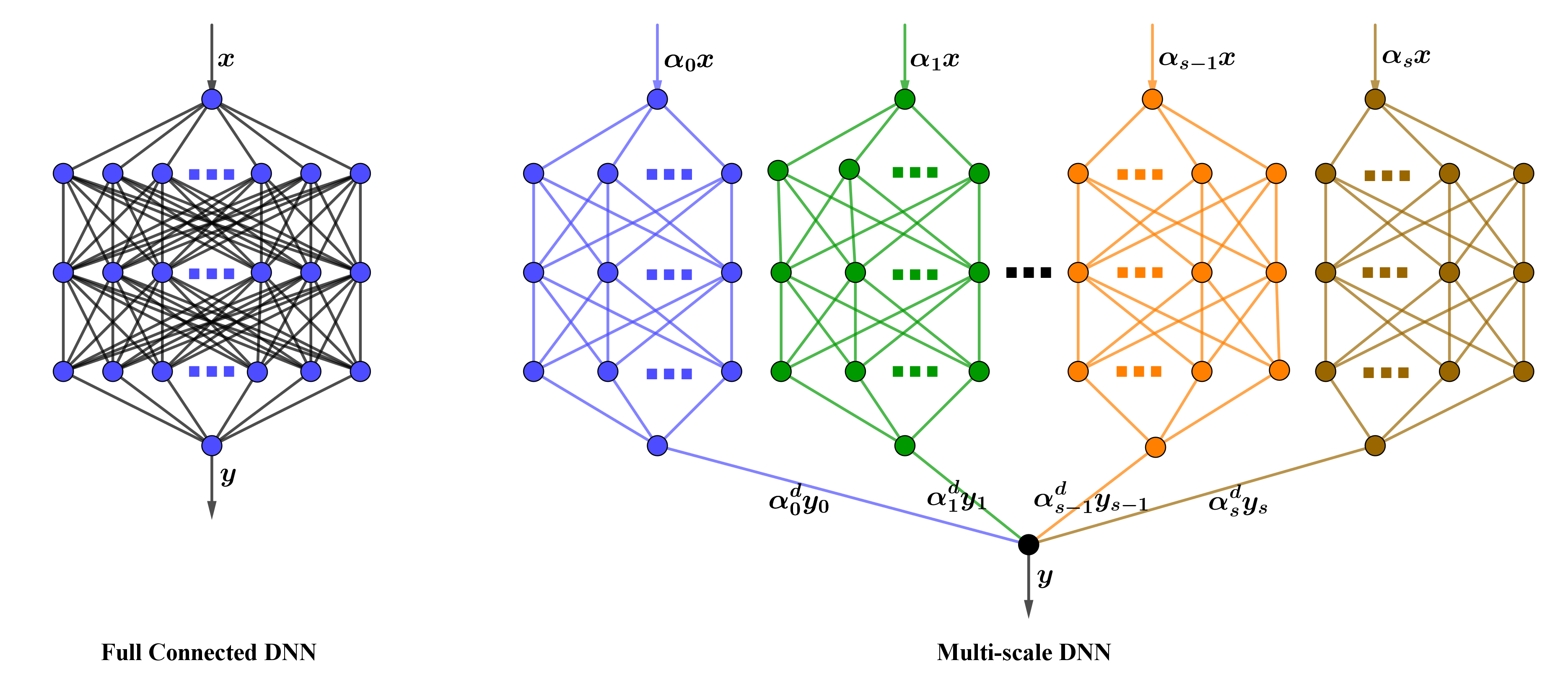
can be expected to have a more uniform convergence and less spectral bias, i.e., frequency uniform approximation to any band-limited function . Deep neural networks defined by (12) are named as the MscaleDNN and a schematic comparison between fully connected DNN and MscaleDNN is shown in Fig. 1.
Previous work presented in [6, 30, 47] have shown that the MscaleDNN can reduce spectral bias significantly in learning highly oscillatory functions, however, mathematical analysis on the mechanism has not been presented in the literature. The following analysis will build a foundation for the MscaleDNN and provide a strategy to manipulate the neural networks.
3 Error diffusion equation model of a two-layer MscaleDNN
In this section, the convergence of a machine learning algorithm for -dimensional regression problems with two layers multi-scale neural networks is analyzed. We will show that the evolution of the error can be modeled by a diffusion equation in the Fourier frequency domain as the width of the network goes to infinity and learning rate approaches to zero.
Consider a regression problem with an objective function defined in a bounded domain . The machine learning algorithm with a neural network denoted by and mean square loss
| (13) |
will be discussed in the following analysis.
The gradient descent dynamics based on the loss functional (13) is
| (14) |
where is the learning rate. By regarding as the time step size, the continuum limit dynamics at is
| (15) |
With the mean square loss function (13) and the chain rule of differentiation, we obtain
| (16) |
for the dynamics of the network function , where
| (17) |
is the neural tangent kernel (NTK) proposed in [19].
A multi-scale neural network with one hidden layer (see. Fig. 1 (right)) is given as
| (18) |
where is the number of scales, are the scaling factors, is the number of neurons for each scale, is the total number of neurons in the hidden layer. Apparently, the network includes the standard fully connected neural network with one hidden layer as a special case of . For this two-layer multi-scale neural network, a direct calculation gives its NTK
| (19) |
Setting the activation function
| (20) |
and assuming all the parameters in , are independent random variables of normal distribution, then, by the law of large numbers and identity
we have
| (21) |
Apparently, can replaced by the parameters of any neuron in the hidden layer. According to the analysis in [19], the NTK will be static during the training assuming the width of the neural network tends to infinity. In addition, the limit NTK is also a convolution kernel as presented in [8, 40]. Suppose and are located on the unit sphere, i.e., , then the limit NTK is a function of the angle between and . The NTKs of some multi-scale neural networks with finite width are compared with their infinite width limit in Fig. 2. We can see that the NTK (19) has an limit given above as .
In order to validate the static property of the limit NTK, we train a multi-scale neural network with , to fit a 3-dimensional function in the domain . The scaling parameters are set to be . The NTKs of the multi-scale neural network after training epochs are compared with the limit NTK in Fig. 3. The results clearly show that the NTK is static during training.
Consequently, as the width of the network goes to infinity, the dynamics of the gradient descent learning (16) tends to
| (22) |
where
| (23) |
is the scaled Gaussian function.
Next, we define a zero extension of the error function by
| (24) |
then, the dynamic system (22) can be rewritten as
| (25) |
where an indicator function is used to extend the equation to the whole space.
Existing works on DNN convergence analysis employ a discrete version of (25) in the physical space by analyzing the eigenvalues of the Gram matrix [43, 32, 36, 40, 23]. However, to get a precise information on the spectral bias phenomena, it is more natural to study the convergence behavior in the Fourier domain as follows.
Given any , the Fourier transform defined in (1) has the following identities
| (26) |
and
| (27) |
In addition, given two functions , , their cross-correlation and convolution are defined as
| (28) |
and we have teh following identities,
| (29) |
Taking Fourier transform (1) on both sides of (25) with respect to and then applying (26)-(29) to rearrange the terms gives a integral-differential equation
| (30) |
where
| (31) |
The convolution with makes the model too complicate to analyze. Nevertheless, if we consider the limit of infinite large domain, i.e., , the limit of is the Dirac delta function and then (30) simplifies to
| (32) |
Define
| (33) |
and denote by the real and imaginary parts of , i.e.,
(Diffusion Model) As the coefficients in (32) are real valued functions, we can rewrite (32) into two independent equations
| (34) |
with respect to the real and imaginary parts of , respectively.
A simpler diffusion equation can be derived if the bias are set to zero in the network. In fact, a function represented by the network without bias has the form
| (35) |
and the neural tangent kernel is given by
| (36) |
Setting the activation function again, and assuming all the parameters are independent random variables of normal distribution, then, by law of large numbers, we have
| (37) |
As the width of the network goes to infinity, the dynamics of the gradient descent learning tends to
| (38) |
Mimicking the derivation for (32), we obtain from (38) that
| (39) |
where . The dynamic system (38) in the Fourier frequency domain implies that only the imaginary part of the error evolves during the gradient descent training if a two layer multi-scale neural network with activation function and zero bias is used. This conclusion is consistent with the fact that the network function (35) can only be used to fit odd functions. Actually, the necessity of non-zero biases in a two layer neural network has been emphasized in [40, 23].
Note that defined in (33) are positive functions in . Therefore, the solution of (34) has an energy equality
| (40) |
which implies that the solution for any as . That means the gradient descent learning for a fitting problem with one hidden layer neural network is convergent assuming that the learning rate is sufficiently small and the width of the neural network is sufficiently large. It is clear that the diffusion coefficients plays a key role in the error decay speed. Several plots of the coefficients are given in Fig. 4 for different scales. We can see that both and have larger support and maximum values with an increasing scale . This implies that larger will leads to fast error reduction in a wider frequency region.
4 Spectral bias analysis of a two layer MscaleDNN using the diffusion equation model
The analysis in previous section has shown that the error dynamics of the gradient descent learning can be approximately described by the diffusion equations (34) in the Fourier spectral domain when the network width and the domain size go to infinity and the learning rate to zero. In this section, we will first propose a Hermite spectral method to obtain highly accurate numerical solutions of the diffusion equation. Some numerical results will be presented to show that the error dynamics predicted by the diffusion model matches well with that of the MscaleDNN during realistic training. Moreover, the results also validate the capability of spectral bias reduction of the MscaleDNNs for wider range of frequencies. For simplicity, we only consider the 1-dimensional case to illustrate the main results.
4.1 Hermite spectral method for the diffusion equation problem
In order to examine quantitatively the decay of the error in the Fourier domain, we will solve numerically the equations in (34) with a Hermite spectral method for the -variable of the equations in (34) on the unbounded computational domain. For this purpose, we introduce the Hermite functions (cf. [41]) defined by
| (41) |
where are Hermite polynomials. The Hermite functions are orthogonal
| (42) |
where is Kronecker symbol.
We discretize the computational time interval into equally-spaced intervals for , where . Then, the Hermite spectral method together with backward Euler time discretization is to find approximation
| (43) |
for at time s.t.,
| (44) |
for all . Here, is a scaling parameter to achieve resolution near , and the bilinear form is defined as
| (45) |
Next, with the unknown vector denoted by , the numerical scheme (44) gives a linear system
| (46) |
where , , are matrices with entries given by
| (47) |
By using the recurrence formula of the Hermite functions, formulations for the matrices , can be derived analytically (see the appendix A).
4.2 Spectral bias reduction of a two layer MscaleDNN
Some numerical examples will be presented to show the capability of the diffusion model in predicting the error dynamics of a two layer MscaleDNN. The predicted results will be compared with the training error of the two-layer MscaleDNN with a large network width and sine activation function. The spectral bias reduction phenomena of MscaleDNNs is validated by the numerical solution of the diffusion model.
Test 1 (Decaying behavior predicted by the diffusion model). We first study the decay speed and range of the solution of the diffusion model (34). Considering an initial condition for the error function in the frequency domain
| (48) |
we will test the diffusion model (34) with three sets of coefficients , . For the numerical discretization of the PDE, we take , in (43). The numerical solutions at different time are plotted in Fig. 5. The numerical results clearly show that the initial error function decays faster over wider frequency ranges with an increasing of . It is worthy to emphasize that diffusion coefficients only produce fast decay in only a small neighborhood of the zero frequency, which corresponds to exactly the spectral bias of a fully connected DNN [37, 51]. These observations are consistent with the performance of the MscaleDNN, which has faster convergence in the approximation of highly oscillated functions.
Test 2 (Validation of error diffusion model with real MscaleDNN training). In this test, we will show that the error dynamics of a finite but wide enough 2-layered multi-scale neural network can be predicted by the diffusion equation model quite well.
We consider a fitting problem with an objective function
| (49) |
on the interval . The Fourier transform of with zero extension outside is
For the two layers multi-scale neural network, the Fourier transform of with zero extension outside can be calculated as
where
and
We will show that the error of the MscaleDNN by the gradient descent learning agrees with that predicted by the diffusion equation (34). We take , , and the initial errors are given by with parameters initialized by sampling from independent random variables of normal distribution. In the gradient descent training for the , the training data set consists of uniformly distributed points in and learning rate is adopted. In this example, a two layers neural network with , and scale is tested and the training is performed in full batch.
Meanwhile, in the Fourier spectral domain, the diffusion equation (34) with initial function will be solved with a -th order the Hermite spectral method introduced above. We take and in the discretization.
The Fourier transform of , denoted by
are compared with at , see Fig. 6. Although many approximations have been used in deriving the diffusion model, the results show that the prediction produced by the diffusion model captured the main features of the error over a long time training process.
On the other hand, we can also compare the training error with the diffusion model prediction in the physical domain. Using the fact that [13, 24]
| (50) |
the Hermite approximation of the error predicted by the diffusion model, i.e.,
| (51) |
can be analytically transformed back to the physical domain as
| (52) |
Then, in the physical domain the errors from the MscaleDNN training and predicted by the diffusion equation can be compared in Fig. 7. Clearly, the evolution of the errors matches quite well in physical domain. It is worthy to point out that the fitting domain is not large. However, the diffusion model can still be a satisfactory predictor for the real error through the training of the MScaleDNN with a large enough network width.
Test 3 (Reduction of spectral bias predicted by error diffusion model). With the confirmation of predicting capability of the diffusion equation model (34) for the error decay of the MscaleDNN with a large enough network width, we will use the model to demonstrate the spectral bias reduction of MscaleDNNs with increasing scales.
Again, We set the network width at , and , and the initial errors are given by with parameters initialized by sampling from independent random variables of normal distribution. In the Hermite spectral method approximation of the diffusion equation (34), we take and . The numerical solution of the diffusion equations at different time for a standard fully connected network (FCN) corresponding to coefficients and a 3-scales MscaleDNN corresponding to coefficients are plotted in Fig. 6-Fig. 7. We can see clearly that FCN with diffusion coefficients only produce decay in a very small neighborhood of the zero frequency while the 3-scale MscaleDNN with coefficients produce much faster decay in a larger frequency interval. Although the initial errors at are different, for FCN and for 3-scale MscaleDNN, the numerical results all verify that multi-scale neural networks has better performance in spectral bias reduction compared with the FCN.
5 Conclusion and future work
In this paper, we investigated the convergence and spectral bias reduction properties of a two-layer multi-scale neural network for regression problems by deriving diffusion equation models in the frequency domain for predicting its error evolution. With the sine activation function, the gradient descent learning of MscaleDNNs leads to the diffusion equation models for the error assuming that the width of the neural network goes to infinity, the learning rate to zero and the fitting domain to the whole space. The diffusion coefficients of the diffusion equations are shown to have wider support in the frequency domain with more scales used in the MscaleDNNs, resulting in a reduction of spectral bias for the MscaleDNNs. This is consistent with the performance of the MscaleDNN with faster convergence in approximating highly oscillated functions from various applications. Moreover, the derived diffusion equation can predict the convergence of the MscaleDNNs learning algorithm even with a finite and reasonably wide network in a finite domain.
The analysis of the MScaleDNNs with more layers, and other popular activation functions, e.g., ReLU, Sigmoid, etc, will be studied following a similar approach of this paper.
Acknowledgments
The first and second authors acknowledges the support provided by NSFC (grant 12022104). W. Z. Zhang acknowledges the support provided by NSFC (grant 12201603). The work of W. Cai is supported by the US National Science Foundation grant DMS-2207449.
Appendix A Analytic formula for the computation of matrices
Then, by the recurrence formula (54), we have
| (55) |
and
| (56) | ||||
for all . Therefore,
| (57) |
where Otherwise, for all ,
| (58) |
Noting that
| (59) |
and , are linear combination of Gaussian functions as presented in (33), the computation of and can be reduced to compute the weighted inner products
| (60) |
where is the normalized Hermite polynomial defined by . In fact, for , given in (33), we have
| (61) |
Next, we present formulas for the calculation of the integrals . Given any scaling factor , scaled Hermite polynomial can be represented by as follows
| (62) |
where can be calculated via recurrence formulas (67). Therefore,
| (63) | ||||
Next, we derive recurrence formulas for the computation of the coefficients . We drop the explicit dependence on without confusion in the following derivation. By the definition of and the recurrence formula (53), we have
| (64) |
Substituting the expansion (62) into (64) gives for
| (65) |
Noting that
| (66) |
direct calculation from (65) gives
Therefore, (65) can be rearranged into
Matching the coefficients on both sides of the above equation gives us
| (67) | ||||
for all , while the initial values are given by
| (68) |
By induction, has explicit formula for all
| (69) |
References
- [1] A. Anandkumar, K. Azizzadenesheli, K. Bhattacharya, N. Kovachki, Z. Y. Li, B. Liu, and A. Stuart. Neural operator: Graph kernel network for partial differential equations. In In: ICLR 2020 Workshop on Integration of Deep Neural Models and Differential Equations, 2020.
- [2] S. Arora, S. Du, W. Hu, Z. Y. Li, and R. Wang. Fine-grained analysis of optimization and generalization for overparameterized two-layer neural networks. In International Conference on Machine Learning, pages 322–332. PMLR, 2019.
- [3] C. Beck, W. E, and A. Jentzen. Machine learning approximation algorithms for high-dimensional fully nonlinear partial differential equations and second-order backward stochastic differential equations. J. Nonlinear Sci., 29:1563–1619, 2019.
- [4] W. Cai, DeepMartNet – A Martingale based deep neural network learning algorithm for eigenvalue/BVP problems and optimal stochastic controls, arXiv preprint arXiv:2307.11942v3, August, 2023.
- [5] W. Cai, X. G. Li, and L. Z. Liu. A phase shift deep neural network for high frequency approximation and wave problems. SIAM J. Sci. Comput., 42(5):A3285–A3312, 2020.
- [6] W. Cai, Z.Q. Xu. Multi-scale deep neural networks for solving high dimensional PDEs. arXiv preprint arXiv:1910.11710. 2019 Oct 25.
- [7] F. Chen, J. Huang, C. Wang, H. Yang. Friedrichs learning: Weak solutions of partial differential equations via deep learning. SIAM Jour. on Scientific Computing. 2023 Jun 30;45(3):A1271-99.
- [8] Y. Cho and L. Saul. Kernel methods for deep learning. NeurIPS, 22:295–301, 2009.
- [9] M. Dissanayake and N. Phan-Thien. Neural-network-based approximations for solving partial differential equations. Commun. Numer. Meth. En., 10(3):195–201, 1994.
- [10] W. E, J. Han, A. Jentzen. Deep learning-based numerical methods for high-dimensional parabolic partial differential equations and backward stochastic differential equations. Commun. Math. Stat., 5(4):349–380, 2017.
- [11] W. E. and B. Yu. The deep ritz method: a deep learning-based numerical algorithm for solving variational problems. Commun. Math. Stat., 6(1):1–12, 2018.
- [12] W. E, C. Ma, L. Wu Machine learning from a continuous viewpoint, i. Sci. China Math., 63(11):2233–2266, 2020.
- [13] I. S. Gradshteyn and I. M. Ryzhik. Table of integrals, series, and products. Academic press, 2014.
- [14] D. Greenfeld, M. Galun, R. Basri, I. Yavneh, and R. Kimmel. Learning to optimize multigrid pde solvers. In In: International Conference on Machine Learning, pages 2415–2423. PMLR, 2019.
- [15] J. Han, A. Jentzen, and W. E. Solving high-dimensional partial differential equations using deep learning. Proc. Nat. Acad. Sci., 115(34):8505–8510, 2018.
- [16] J. Han and J. H. Long. Convergence of the deep bsde method for coupled fbsdes. Probab. Uncertain. Quant. Risk, 5:1–33, 2020.
- [17] J. T. Hsieh, S. J. Zhao, S. Eismann, L. Mirabella, and S. Ermon. Learning neural PDE solvers with convergence guarantees. In: International Conference on Learning Representations, 2018.
- [18] T. H. Hu, B. T. Jin, and Z. Zhou. Solving elliptic problems with singular sources using singularity splitting deep Ritz method. arXiv preprint arXiv:2209.02931, 2022.
- [19] A. Jacot, F. Gabriel, and C. Hongler. Neural tangent kernel: Convergence and generalization in neural networks. Proc. Adv. Neural Inf. Process. Syst., 31, 2018.
- [20] A. Krizhevsky, I. Sutskever, and G. E. Hinton. Imagenet classification with deep convolutional neural networks. In: Advances in Neural Information Processing Systems 25 (NeurIPS 2012), pages 1097–1105, 2012.
- [21] I. E. Lagaris, A. Likas, and D. I. Fotiadis. Artificial neural networks for solving ordinary and partial differential equations. IEEE Trans. Neural Networks, 9(5):987–1000, 1998.
- [22] I. Lauriola, A. Lavelli, and F. Aiolli. An introduction to deep learning in natural language processing: Models, techniques, and tools. Neurocomputing, 470:443–456, 2022.
- [23] J. Lee, L. Xiao, S. Schoenholz, Y. Bahri, R. Novak, J. Sohl-Dickstein, and J. Pennington. Wide neural networks of any depth evolve as linear models under gradient descent. NeurIPS, 32, 2019.
- [24] H. Y. Li, R. Q. Liu, and L. L. Wang. Efficient hermite spectral-Galerkin methods for nonlocal diffusion equations in unbounded domains. Numer. Math-Theory Me., 2022.
- [25] X. A. Li, Z. Q. John Xu, and L. Zhang. A multi-scale dnn algorithm for nonlinear elliptic equations with multiple scales. Commun. Comput. Phys., 28:1886–1906, 2020.
- [26] Z. Y. Li, N. Kovachki, K. Azizzadenesheli, B. Liu, K. Bhattacharya, A. Stuart, and A. Anandkumar. Fourier neural operator for parametric partial differential equations. In: International Conference on Learning Representations, 2021.
- [27] Z. Y. Li, N. Kovachki, K. Azizzadenesheli, B. Liu, A. Stuart, K. Bhattacharya, and A. Anandkumar. Multipole graph neural operator for parametric partial differential equations. In: Advances in Neural Information Processing Systems, 33:6755–6766, 2020.
- [28] Y. Liao and P. Ming. Deep Nitsche method: Deep Ritz method with essential boundary conditions. arXiv preprint arXiv:1912.01309, 2019.
- [29] Y. J. Liu and C. Yang. Vpvnet: a velocity-pressure-vorticity neural network method for the stokes’ equations under reduced regularity. arXiv preprint arXiv:2112.07131, 2021.
- [30] Z. Q. Liu, W. Cai, and John Z. Q. Xu. Multi-scale deep neural network (MscaleDNN) for solving poisson-boltzmann equation in complex domains. Commun. Comput. Phys., 28(5):1970–2001, 2020.
- [31] D. H. Lu, K. Popuri, Gavin W. Ding, R. Balachandar, and M. F. Beg. Multimodal and multiscale deep neural networks for the early diagnosis of alzheimer’s disease using structural mr and fdg-pet images. Sci. Rep., 8(1):5697, 2018.
- [32] T. Luo, Z. Ma, Z. Q. John Xu, and Y. Zhang. On the exact computation of linear frequency principle dynamics and its generalization. SIAM J. Math. Data Sci., 4(4):1272–1292, 2022.
- [33] B. Mildenhall, P. P. Srinivasan, M. Tancik, J. T. Barron, R. Ramamoorthi, and R. Ng. Nerf: Representing scenes as neural radiance fields for view synthesis. Commun. ACM, 65(1):99–106, 2021.
- [34] J. Müller and M. Zeinhofer. Deep ritz revisited. arXiv preprint arXiv:1912.03937, 2019.
- [35] D. W. Otter, J. R Medina, and J. K. Kalita. A survey of the usages of deep learning for natural language processing. IEEE Trans. Neural Netw. Learn. Syst., 32(2):604–624, 2020.
- [36] Y. Peng, D. Hu, and Z. Q. John Xu. A non-gradient method for solving elliptic partial differential equations with deep neural networks. J. Computat. Phys., 472:111690, 2023.
- [37] N. Rahaman, A. Baratin, D. Arpit, F. Draxler, M. Lin, F. Hamprecht, Y. Bengio, and A. Courville. On the spectral bias of neural networks. In International Conference on Machine Learning, pages 5301–5310. PMLR, 2019.
- [38] M. Raissi and G. E. Karniadakis. Hidden physics models: Machine learning of nonlinear partial differential equations. J. Comput. Phys., 357:125–141, 2018.
- [39] M. Raissi, P. Perdikaris, and G. E. Karniadakis. Physics-informed neural networks: A deep learning framework for solving forward and inverse problems involving nonlinear partial differential equations. J. Computat. Phys., 378:686–707, 2019.
- [40] B. Ronen, D. Jacobs, Y. Kasten, and S. Kritchman. The convergence rate of neural networks for learned functions of different frequencies. NeurIPS, 32, 2019.
- [41] J. Shen, T. Tang, and L.L. Wang. Spectral Methods: Algorithms, Analysis and Applications, volume 41 of Springer Series in Computational Mathematics. Springer-Verlag, 2011.
- [42] K. Simonyan and A. Zisserman. Very deep convolutional networks for large-scale image recognition. In: Proceedings of the 2015 Int. Conf. on Learning Representations (ICLR), 2015.
- [43] M. Tancik, P. Srinivasan, B. Mildenhall, S. Fridovich-Keil, N. Raghavan, U. Singhal, R. Ramamoorthi, J. Barron, and R. Ng. Fourier features let networks learn high frequency functions in low dimensional domains. In: Advances in Neural Information Processing Systems, 33:7537–7547, 2020.
- [44] B. B. Traore, B. Kamsu-Foguem, and F. Tangara. Deep convolution neural network for image recognition. Ecol. Inform., 48:257–268, 2018.
- [45] R. Tsuchida, F. Roosta, and M. Gallagher. Invariance of weight distributions in rectified mlps. In International Conference on Machine Learning, pages 4995–5004. PMLR, 2018.
- [46] K. Um, R. Brand, Y. R. Fei, P. Holl, and N. Thuerey. Solver-in-the-loop: Learning from differentiable physics to interact with iterative PDE-solvers. In: Advances in Neural Information Processing Systems, 33:6111–6122, 2020.
- [47] B. Wang, W. Z. Zhang, and W. Cai. Multi-scale deep neural network (MscaleDNN) methods for oscillatory stokes flows in complex domains. Commun. Comput. Phys., 28(5):2139–2157, 2020.
- [48] S. Wang, H. Wang, P. Perdikaris. On the eigenvector bias of Fourier feature networks: From regression to solving multi-scale PDEs with physics-informed neural networks. Computer Methods in Applied Mechanics and Engineering. 2021 Oct 1;384:113938.
- [49] C. Williams. Computing with infinite networks. NeurIPS, 9:295–301, 1996.
- [50] B. Xie, Y. Liang, and L. Song. Diverse neural network learns true target functions. In Artificial Intelligence and Statistics, pages 1216–1224. PMLR, 2017.
- [51] Z. Q. J. Xu, Y. Y. Zhang, T. Luo, Y. Y. Xiao, and Z. Ma. Frequency principle: Fourier analysis sheds light on deep neural networks. Commun. Comput. Phys., 28(5):1746–1767, 2020.
- [52] Z. Q. J. Xu, Y. Zhang, and T. Luo. Overview frequency principle/spectral bias in deep learning. arXiv preprint arXiv:2201.07395, 2022.
- [53] T. Young, D. Hazarika, S. Poria, and E. Cambria. Recent trends in deep learning based natural language processing. IEEE Comput. Intell. M., 13(3):55–75, 2018.
- [54] Y. H. Zang, G. Bao, X. J. Ye, and H. M. Zhou. Weak adversarial networks for high-dimensional partial differential equations. J. Comput. Phys., 411:109409, 2020.
- [55] L. Zhang, W. Cai, and Z. Q. John Xu. A correction and comments on ”multi-scale deep neural network (mscalednn) for solving poisson-boltzmann equation in complex domains. cicp, 28(5):1970–2001,2020”. Commun. Comput. Phys., 33(5):1509–1513, 2023.
- [56] W. Z. Zhang and W. Cai. Fbsde based neural network algorithms for high-dimensional quasilinear parabolic pdes. J. Comput. Phys., 470:111557, 2022.
- [57] E. D. Zhong, T. Bepler, B. Berger, and J. H. Davis. Cryodrgn: reconstruction of heterogeneous cryo-em structures using neural networks. Nat. Methods, 18(2):176–185, 2021.