跳到论文正文
W Papers独立论文阅读器 arXiv:2212.03225 论文正文 计算阅读时间 · 0%
引用这篇论文根据当前论文元数据生成,正式投稿前建议核对。


License: arXiv.org perpetual non-exclusive license
arXiv:2212.03225v1 [math.OC] 06 Dec 2022

Robust Local Stabilization of Nonlinear Systems with Controller-Dependent Norm Bounds: A Convex Approach with Input-Output Sampling

Sze Kwan Cheah    Diganta Bhattacharjee    Maziar S. Hemati       Ryan J. Caverly Thanks: This work is supported by the Office of the Under Secretary of Defense for Research and Engineering under award number FA9550-21-1-0213. DB and MSH acknowledge partial support from the Air Force Office of Scientific Research under award numbers FA9550-21-1-0106 and FA9550-22-1-0004, the Army Research Office under award number W911NF-20-1-0156, and the National Science Foundation under award number CBET-1943988. (SKC and DB are co-first authors.) Thanks: The authors are with the Department of Aerospace Engineering & Mechanics, University of Minnesota, Minneapolis, MN 55455, USA. Email: {cheah013, dbhattac, mhemati, rcaverly}@umn.edu
Abstract

This letter presents a framework for synthesizing a robust full-state feedback controller for systems with unknown nonlinearities. Our approach characterizes input-output behavior of the nonlinearities in terms of local norm bounds using available sampled data corresponding to a known region about an equilibrium point. A challenge in this approach is that if the nonlinearities have explicit dependence on the control inputs, an a priori selection of the control input sampling region is required to determine the local norm bounds. This leads to a “chicken and egg” problem, where the local norm bounds are required for controller synthesis, but the region of control inputs needed to be characterized cannot be known prior to synthesis of the controller. To tackle this issue, we constrain the closed-loop control inputs within the sampling region while synthesizing the controller. As the resulting synthesis problem is non-convex, three semi-definite programs (SDPs) are obtained through convex relaxations of the main problem, and an iterative algorithm is constructed using these SDPs for control synthesis. Two numerical examples are included to demonstrate the effectiveness of the proposed algorithm.

I Introduction

A large portion of the existing literature on nonlinear control comprises model-based approaches (e.g., backstepping, feedback linearization [1]) that depend on the availability of a sufficiently accurate analytical model of the system or plant to be controlled. There is an inherent assumption that such an analytic model can be obtained from the fundamental laws governing the system. However, there are many instances where a reliable and/or accurate analytical model of the system cannot be obtained in practice. Robust control theory can also be used to design a stabilizing controller for a nonlinear system under the assumption that at least a nominal realization of the system, either linear time-invariant (LTI) or linear time-varying (LTV), can be obtained (see, e.g., [2, 3, 4, Chapter 9]). In this setting, the system is described in linear fractional transformation (LFT) form, where the nominal system is connected in feedback with a ‘perturbation’ that captures all aspects of the system that do not fit within an LTI or LTV framework (e.g., nonlinearity, uncertainty, time delays). The control synthesis is then based on the input-output (I/O) properties of the perturbation, which are assumed to hold for some known structure and/or set of perturbations (e.g., integral quadratic constraints [5], structured singular value [6]). For a complex system, however, it is not trivial to quantify these I/O properties and ascertain if the accompanying assumptions hold, especially when the analytical form of the perturbation is not explicitly known.

Data-driven techniques are now becoming increasingly popular to overcome these issues[7]. For example, strategies are being proposed for determining I/O properties from sampled data (like dissipation inequalities [8] and passivity [9]). Also, data-driven approaches for robust control, with a focus on perturbations representing parametric uncertainties and unknown nonlinearity driven by states and/or parameters, are gaining popularity [10, 11, 12]. However, the class of perturbations for which the unknown nonlinearity is a function of both the states and control inputs is relatively less studied. Existing data-driven methods for this class of perturbations are either guaranteed to work in a small neighborhood of the equilibrium [13] or require extensive tuning of the associated control parameters to satisfy the underlying assumptions [14]. In light of these challenges associated with purely data-driven control, we have adopted an approach where I/O properties of the perturbation are established through data and subsequently used for control synthesis.

We consider a general nonlinear system and partition it into an LFT form, where the nominal system captures the system’s LTI dynamics about an equilibrium and the perturbation comprises higher-order nonlinearities, which are functions of both the states and control inputs and are not necessarily known analytically. Assuming I/O samples of the perturbation are available, local norm bounds are derived. A robust state-feedback controller is synthesized that asymptotically stabilizes the nonlinear system locally within the sampled region for all perturbations satisfying the norm bounds. Since the norm bounds, which depend on control inputs, are used in the synthesis, the synthesized controller must ensure that the control inputs remain within the sampling set. Moreover, the main synthesis problem involves non-convex constraints. We relax the main problem into three semi-definite programs (SDPs) that are solved iteratively. To summarize, the contribution of this work is an iterative control synthesis method that results in local asymptotic stabilization of a nonlinear system, where the system’s nonlinearities are analytically unknown, but available through sampling, and depend explicitly on control inputs.

Notation: The symbol 𝒩n\mathcal{N}_{n} is a shorthand for the set {1,2,…,n}\{1,2,\dots,n\}, and ‖⋅‖\left\|\cdot\right\| denotes the 2-norm for vectors and spectral norm for matrices. An nn-dimensional vector of zeros with the ii-th entry equal to one is denoted by 𝟏𝐧𝐢\mbf{1}_{n_{i}}. We use 𝐀>𝟎\mbf{A}>0 to denote a symmetric, positive definite matrix 𝐀\mbf{A}. The maximum singular value of 𝐌\mbf{M} is denoted by σ¯​(𝐌)\bar{\sigma}(\mbf{M}). For a given 𝐄>𝟎\mbf{E}>0, an ellipsoid centered at the origin is denoted by ℰn​(𝐄)={𝐱∈ℝ𝐧|‖𝐄−𝟏​𝐱‖≤𝟏}\mathcal{E}_{n}(\mbf{E})=\{\mbf{x}\in\mathbb{R}^{n}|\left\|\mbf{E}^{-1}\mbf{x}\right\|\leq 1\}. Finally, ℬn\mathcal{B}_{n} denotes the closed unit-norm ball in ℝn\mathbb{R}^{n}.

II Problem Formulation

Consider a nonlinear dynamic system of the form

𝐱˙=𝐟⁡(𝐱,𝐮),\dot{\mbf{x}}=\mbf{f}(\mbf{x},\mbf{u}), (1)

where 𝐱∈ℝ𝐧𝐱\mbf{x}\in\mathbb{R}^{n_{x}} and 𝐮∈ℝ𝐧𝐮\mbf{u}\in\mathbb{R}^{n_{u}} are the state and control input vectors, respectively, and 𝐟:ℝ𝐧𝐱×ℝ𝐧𝐮→ℝ𝐧𝐱\mbf{f}:\mathbb{R}^{n_{x}}\times\mathbb{R}^{n_{u}}\rightarrow\mathbb{R}^{n_{x}} is a nonlinear function subject to the following assumption.

Assumption II.1

𝐟\mbf{f} is not precisely known. However, there exists at least one equilibrium (𝐱𝟎,𝐮𝟎)(\mbf{x}_{0},\mbf{u}_{0}) such that 𝐟⁡(𝐱𝟎,𝐮𝟎)=𝟎\mbf{f}(\mbf{x}_{0},\mbf{u}_{0})=\mbf{0}, and 𝐀=∂𝐟∂𝐱|(𝐱𝟎,𝐮𝟎)\mbf{A}=\frac{\partial\mbf{f}}{\partial\mbf{x}}|_{(\mbf{x}_{0},\mbf{u}_{0})}, 𝐁𝟏=∂𝐟∂𝐮|(𝐱𝟎,𝐮𝟎)\mbf{B}_{1}=\frac{\partial\mbf{f}}{\partial\mbf{u}}|_{(\mbf{x}_{0},\mbf{u}_{0})} are known.

All the developments in this letter are based on the above assumption. If multiple equilibria are known, we choose the one that is relevant for the problem at hand. Next, by setting 𝐱=𝐱𝟎+δ​𝐱\mbf{x}=\mbf{x}_{0}+\delta\mbf{x}, 𝐮=𝐮𝟎+δ​𝐮\mbf{u}=\mbf{u}_{0}+\delta\mbf{u}, we can rewrite (1) as

δ​𝐱˙=𝐀​δ​𝐱+𝐁𝟏​δ​𝐮+𝚫⁡(δ​𝐱,δ​𝐮),\delta\dot{\mbf{x}}=\mbf{A}\delta\mbf{x}+\mbf{B}_{1}\delta\mbf{u}+{\boldsymbol{\Delta}}(\delta\mbf{x},\delta\mbf{u}), (2)

where 𝐀,𝐁𝟏\mbf{A},\mbf{B}_{1} are as defined in Assumption II.1, and 𝚫:ℝnx×ℝnu→ℝnx{\boldsymbol{\Delta}}:\mathbb{R}^{n_{x}}\times\mathbb{R}^{n_{u}}\rightarrow\mathbb{R}^{n_{x}} is a function that captures the higher-order terms. Note that 𝚫{\boldsymbol{\Delta}}, whose analytical form is not available, is a function of both δ​𝐱,δ​𝐮\delta\mbf{x},\delta\mbf{u}. Also, we assume that 𝚫{\boldsymbol{\Delta}} is memoryless and static. Thus, system (2) can be expressed in an LFT form having the nominal LTI dynamics δ​𝐱˙=𝐀​δ​𝐱+𝐁𝟏​δ​𝐮\delta\dot{\mbf{x}}=\mbf{A}\delta\mbf{x}+\mbf{B}_{1}\delta\mbf{u} and the perturbation 𝚫{\boldsymbol{\Delta}}.

Although 𝚫{\boldsymbol{\Delta}} is not known analytically, we assume that a finite number of input-output samples of 𝚫{\boldsymbol{\Delta}} are available from either experiments or high-fidelity numerical simulations. We also assume that the sampling is carried out in a known region around the equilibrium, such as over a NN-point grid where NN is large. We refer to this region as the sampling region 𝒮=𝕏×𝕌,\mathcal{S}=\mathbb{X}\times\mathbb{U}, where 𝕏⊂ℝnx\mathbb{X}\subset\mathbb{R}^{n_{x}} and 𝕌⊂ℝnu\mathbb{U}\subset\mathbb{R}^{n_{u}} are known, compact sets that contain the respective origins in the interiors. Therefore, we have access to NN input-output samples {(δ​𝐱(𝐤),δ​𝐮(𝐤)),𝚫⁡(δ​𝐱(𝐤),δ​𝐮(𝐤))}k∈𝒩N\{\left(\delta\mbf{x}^{(k)},\delta\mbf{u}^{(k)}\right),{\boldsymbol{\Delta}}\left(\delta\mbf{x}^{(k)},\delta\mbf{u}^{(k)}\right)\}_{k\in\mathcal{N}_{N}}, where (δ​𝐱(𝐤),δ​𝐮(𝐤))∈𝒮\left(\delta\mbf{x}^{(k)},\delta\mbf{u}^{(k)}\right)\in\mathcal{S} for all k∈𝒩Nk\in\mathcal{N}_{N}. Upon investigating these samples, we can deduce the following:

  • •

    If the vector 𝚫⁡(δ​𝐱(𝐤),δ​𝐮(𝐤)){\boldsymbol{\Delta}}\left(\delta\mbf{x}^{(k)},\delta\mbf{u}^{(k)}\right) corresponding to δ​𝐱(𝐤)≠𝟎\delta\mbf{x}^{(k)}\neq\mbf{0} and δ​𝐮(𝐤)≠𝟎\delta\mbf{u}^{(k)}\neq\mbf{0} contains elements that are identically 0, then the original system (1) has states that are governed by purely LTI dynamics. This, in conjunction with the nonzero entries (say, nwn_{w} of those), can be used to find a realization of 𝚫⁡(δ​𝐱(𝐤),δ​𝐮(𝐤)){\boldsymbol{\Delta}}\left(\delta\mbf{x}^{(k)},\delta\mbf{u}^{(k)}\right) of the form 𝚫⁡(δ​𝐱(𝐤),δ​𝐮(𝐤))=[Δ1⋯0Δnw⋯]𝖳,{\boldsymbol{\Delta}}\left(\delta\mbf{x}^{(k)},\delta\mbf{u}^{(k)}\right)=\begin{bmatrix}\Delta_{1}&\cdots&0&\Delta_{n_{w}}&\cdots\end{bmatrix}^{\mathsf{T}}, where Δi:ℝnx×ℝnu→ℝ,i∈𝒩nw\Delta_{i}:\mathbb{R}^{n_{x}}\times\mathbb{R}^{n_{u}}\rightarrow\mathbb{R},\ i\in\mathcal{N}_{n_{w}} are the nonlinearties corresponding to the nonzero entries. Thus, the above can be reformulated as 𝚫⁡(δ​𝐱(𝐤),δ​𝐮(𝐤))=𝐁𝟐​𝐰(𝐤){\boldsymbol{\Delta}}\left(\delta\mbf{x}^{(k)},\delta\mbf{u}^{(k)}\right)=\mbf{B}_{2}\mbf{w}^{(k)} where 𝐰(𝐤)=[𝐰𝟏(𝐤)𝐰𝟐(𝐤)…𝐰𝐧𝐰(𝐤)]𝖳∈ℝ𝐧𝐰\mbf{w}^{(k)}=\begin{bmatrix}w_{1}^{(k)}&w_{2}^{(k)}&\ldots&w_{n_{w}}^{(k)}\end{bmatrix}^{\mathsf{T}}\in\mathbb{R}^{n_{w}} contains outputs of all the nonlinearities and 𝐁𝟐∈ℝ𝐧𝐱×𝐧𝐰\mbf{B}_{2}\in\mathbb{R}^{n_{x}\times n_{w}} properly distributes the elements of 𝐰(𝐤)\mbf{w}^{(k)}.

  • •

    We can also identify the individual states and control inputs that drive each nonlinear function Δi\Delta_{i}. Based on this, the sampled input to Δi\Delta_{i} takes the form 𝐯𝐢(𝐤)=[δ𝐱𝟏(𝐤)⋯ 0⋯δ𝐮𝟏(𝐤)⋯ 0⋯]𝖳∈ℝ𝐧𝐱+𝐧𝐮\mbf{v}_{i}^{(k)}=\left[\delta x_{1}^{(k)}\ \cdots\ 0\ \cdots\ \delta u_{1}^{(k)}\ \cdots\ 0\ \cdots\right]^{\mathsf{T}}\in\mathbb{R}^{n_{x}+n_{u}} which is equivalent to 𝐯𝐢(𝐤)=𝐂𝐢​δ​𝐱(𝐤)+𝐃𝐢​δ​𝐮(𝐤)\mbf{v}_{i}^{(k)}=\mbf{C}_{i}\delta\mbf{x}^{(k)}+\mbf{D}_{i}\delta\mbf{u}^{(k)} with 𝐂𝐢∈ℝ(𝐧𝐱+𝐧𝐮)×𝐧𝐱,𝐃𝐢∈ℝ(𝐧𝐱+𝐧𝐮)×𝐧𝐮\mbf{C}_{i}\in\mathbb{R}^{(n_{x}+n_{u})\times n_{x}},\ \mbf{D}_{i}\in\mathbb{R}^{(n_{x}+n_{u})\times n_{u}} known. Therefore, for each k∈𝒩Nk\in\mathcal{N}_{N}, we have wi(k)=Δi​(𝐯𝐢(𝐤)),𝐢∈𝒩𝐧𝐰w_{i}^{(k)}=\Delta_{i}(\mbf{v}_{i}^{(k)}),\ i\in\mathcal{N}_{n_{w}}. Although expressed in this form, it is understood that each Δi\Delta_{i} maps ℝnx×ℝnu\mathbb{R}^{n_{x}}\times\mathbb{R}^{n_{u}} to ℝ\mathbb{R}.

  • •

    The samples can be used to prescribe empirical norm bounds on the inputs-outputs of each Δi\Delta_{i}. Specifically, we intend to find γi>0\gamma_{i}>0 for each i∈𝒩nwi\in\mathcal{N}_{n_{w}} such that (wi(k))2≤γi2​‖𝐯𝐢(𝐤)‖2\left(w_{i}^{(k)}\right)^{2}\leq\gamma_{i}^{2}\left\|\mbf{v}_{i}^{(k)}\right\|^{2} holds for all k∈𝒩Nk\in\mathcal{N}_{N}. To this end, for each pair (i,k)∈𝒩nw×𝒩N(i,k)\in\mathcal{N}_{n_{w}}\times\mathcal{N}_{N}, we define γi(k)=((wi(k))2/‖𝐯𝐢(𝐤)‖2)1/2\gamma_{i}^{(k)}=\left(\left(w_{i}^{(k)}\right)^{2}\big/\left\|\mbf{v}_{i}^{(k)}\right\|^{2}\right)^{1/2} and stack all such bounds in a matrix Γ=[Γ1Γ2⋯Γnw],\Gamma=\begin{bmatrix}\Gamma_{1}&\Gamma_{2}&\cdots&\Gamma_{n_{w}}\end{bmatrix}, where Γi=[γi(1)γi(2)…γi(N)]𝖳\Gamma_{i}=\begin{bmatrix}\gamma^{(1)}_{i}&\gamma^{(2)}_{i}&\dots&\gamma^{(N)}_{i}\end{bmatrix}^{\mathsf{T}}. The empirical bounds are then specified as the maximum over each column, i.e., γi=max⁡Γi\gamma_{i}=\max\Gamma_{i}. If we seek the bounds over a region 𝔻⊆𝒮\mathbb{D}\subseteq\mathcal{S}, the same procedure can be repeated with the sampled data corresponding to 𝔻\mathbb{D}.

Using the above information, system (2) can be rewritten as

δ​𝐱˙\displaystyle\delta\dot{\mbf{x}} =𝐀​δ​𝐱+𝐁𝟏​δ​𝐮+𝐁𝟐​𝐰,\displaystyle=\mbf{A}\delta\mbf{x}+\mbf{B}_{1}\delta\mbf{u}+\mbf{B}_{2}\mbf{w},
wi\displaystyle w_{i} =Δi​(𝐯𝐢),𝐢∈𝒩𝐧𝐰,\displaystyle=\Delta_{i}(\mbf{v}_{i}),\ i\in\mathcal{N}_{n_{w}}, (3)
𝐯𝐢\displaystyle\mbf{v}_{i} =(𝐂𝐢​δ​𝐱+𝐃𝐢​δ​𝐮),i∈𝒩nw,\displaystyle=\left(\mbf{C}_{i}\delta\mbf{x}+\mbf{D}_{i}\delta\mbf{u}\right),\ i\in\mathcal{N}_{n_{w}},

with the following standing assumption for a given 𝔻⊆𝒮\mathbb{D}\subseteq\mathcal{S}.

Assumption II.2

Let γi,i∈𝒩nw\gamma_{i},\ i\in\mathcal{N}_{n_{w}} be the empirical bounds corresponding to 𝔻\mathbb{D}. Each input-output tuple (𝐯𝐢,𝐰𝐢)\left(\mbf{v}_{i},w_{i}\right) satisfies the bound γi\gamma_{i} in 𝔻\mathbb{D}, i.e., wi2≤γi2​‖𝐯𝐢‖2w_{i}^{2}\leq\gamma_{i}^{2}\left\|\mbf{v}_{i}\right\|^{2}, for all (δ​𝐱,δ​𝐮)∈𝔻\left(\delta\mbf{x},\delta\mbf{u}\right)\in\mathbb{D} and for all i∈𝒩nwi\in\mathcal{N}_{n_{w}}. Also, for each i∈𝒩nwi\in\mathcal{N}_{n_{w}}, let 𝚫𝔻i{\boldsymbol{\Delta}}_{\mathbb{D}_{i}} be the set of functions Δi:𝔻→ℝ\Delta_{i}:\mathbb{D}\rightarrow\mathbb{R} for which the bound γi\gamma_{i} holds.

The above assumption is reasonable since our knowledge is restricted to the extent provided by the sampled data and analytical forms of Δi\Delta_{i}s are unknown. Now, we are interested in designing a state-feedback control law δ​𝐮=𝐊​δ​𝐱\delta\mbf{u}=\mbf{K}\delta\mbf{x} for the open-loop system (3), under Assumption II.2 with 𝔻=𝕏c×𝕌c\mathbb{D}=\mathbb{X}_{c}\times\mathbb{U}_{c} for some 𝕏c⊆𝕏\mathbb{X}_{c}\subseteq\mathbb{X}, 𝕌c⊆𝕌\mathbb{U}_{c}\subseteq\mathbb{U} containing the respective origins in the interiors. The closed-loop system thus becomes

δ​𝐱˙\displaystyle\delta\dot{\mbf{x}} =(𝐀+𝐁𝟏​𝐊)​δ​𝐱+𝐁𝟐​𝐰,\displaystyle=\left(\mbf{A}+\mbf{B}_{1}\mbf{K}\right)\delta\mbf{x}+\mbf{B}_{2}\mbf{w},
wi\displaystyle w_{i} =Δi​(𝐯𝐢),𝐢∈𝒩𝐧𝐰,\displaystyle=\Delta_{i}(\mbf{v}_{i}),\ i\in\mathcal{N}_{n_{w}}, (4)
𝐯𝐢\displaystyle\mbf{v}_{i} =(𝐂𝐢+𝐃𝐢​𝐊)​δ​𝐱,𝐢∈𝒩𝐧𝐰.\displaystyle=\left(\mbf{C}_{i}+\mbf{D}_{i}\mbf{K}\right)\delta\mbf{x},\ i\in\mathcal{N}_{n_{w}}.

The goal is to synthesize 𝐊\mbf{K} to certify the closed-loop system (4) asymptotically stable in the largest local region 𝕏c⊆𝕏\mathbb{X}_{c}\subseteq\mathbb{X}, for a choice of 𝕌c⊆𝕌\mathbb{U}_{c}\subseteq\mathbb{U} and the corresponding bounds γi\gamma_{i} and set of functions 𝚫𝔻i{\boldsymbol{\Delta}}_{\mathbb{D}_{i}}, i∈𝒩nwi\in\mathcal{N}_{n_{w}}. However, as the synthesis uses γi\gamma_{i}, we need to verify whether the closed-loop control trajectories satisfy δ​𝐮=𝐊​δ​𝐱∈𝕌𝐜\delta\mbf{u}=\mbf{K}\delta\mbf{x}\in\mathbb{U}_{c} for 𝐊\mbf{K} to be consistent with the data. This requires the use of an iterative approach, which is described in detail in the synthesis presented in the next section. Before discussing the control synthesis, we outline a few useful matrix inequality results.

Lemma II.1

(Young’s Relation [15]): Consider 𝐗∈ℝ𝐦×𝐧\mbf{X}\in\mathbb{R}^{m\times n} and 𝐘∈ℝ𝐦×𝐧\mbf{Y}\in\mathbb{R}^{m\times n}. For any 𝐒>𝟎\mbf{S}>0, it holds that

𝐗𝖳​𝐘+𝐘𝖳​𝐗≤𝐗𝖳​𝐒−𝟏​𝐗+𝐘𝖳​𝐒𝐘.\displaystyle\mbf{X}^{\mathsf{T}}\mbf{Y}+\mbf{Y}^{\mathsf{T}}\mbf{X}\leq\mbf{X}^{\mathsf{T}}\mbf{S}^{-1}\mbf{X}+\mbf{Y}^{\mathsf{T}}\mbf{S}\mbf{Y}. (5)

A special case of Lemma II.1 that will prove useful in the control synthesis presented in the next section considers 𝐒=𝐈\mbf{S}=\mbf{I}, 𝐗=𝐇∈ℝ𝐧𝐱×𝐧𝐱\mbf{X}=\mbf{H}\in\mathbb{R}^{n_{x}\times n_{x}} and 𝐘=𝐇𝟎∈ℝ𝐧𝐱×𝐧𝐱\mbf{Y}=\mbf{H}_{0}\in\mathbb{R}^{n_{x}\times n_{x}}, which leads to

𝐇𝖳​𝐇\displaystyle\mbf{H}^{\mathsf{T}}\mbf{H} ≥𝐇𝖳​𝐇𝟎+𝐇𝟎𝖳​𝐇−𝐇𝟎𝖳​𝐇𝟎.\displaystyle\geq\mbf{H}^{\mathsf{T}}\mbf{H}_{0}+\mbf{H}^{\mathsf{T}}_{0}\mbf{H}-\mbf{H}^{\mathsf{T}}_{0}\mbf{H}_{0}. (6)

III Control Synthesis

This section describes the synthesis of a static state-feedback controller 𝐊\mbf{K}, which requires breaking the main synthesis problem into different sub-problems and iterating over these sub-problems to obtain a controller that is certified to render the closed-loop system (4) asymptotically stable within 𝕏c\mathbb{X}_{c}. We will start by specifying structures of the sets 𝕏c\mathbb{X}_{c} and 𝕌c\mathbb{U}_{c} that will be used in the remainder of the letter. The local region 𝕏c\mathbb{X}_{c} is taken to be a family of ellipsoids parameterized by 𝐖>𝟎\mbf{W}>0, i.e., 𝕏c=ℰnx​(𝐖)\mathbb{X}_{c}=\mathcal{E}_{n_{x}}(\mbf{W}), where 𝐖\mbf{W} is chosen appropriately such that 𝕏c⊆𝕏\mathbb{X}_{c}\subseteq\mathbb{X}. Similarly, we take 𝕌c=r​ℬnu\mathbb{U}_{c}=r\mathcal{B}_{n_{u}}, where r>0r>0 is the parameter related to the control input magnitude and is chosen such that 𝕌c⊆𝕌\mathbb{U}_{c}\subseteq\mathbb{U}. With these sets defined, the main synthesis problem is summarized in the next result.

Theorem III.1

Let 𝐖>𝟎\mbf{W}>0 and r>0r>0 be chosen such that 𝕏c=ℰnx​(𝐖)⊆𝕏\mathbb{X}_{c}=\mathcal{E}_{n_{x}}(\mbf{W})\subseteq\mathbb{X} and 𝕌c=r​ℬnu⊆𝕌\mathbb{U}_{c}=r\mathcal{B}_{n_{u}}\subseteq\mathbb{U}, respectively. Suppose Assumption II.2 holds with 𝔻=𝕏c×𝕌c\mathbb{D}=\mathbb{X}_{c}\times\mathbb{U}_{c}. Then, the closed-loop system (4) is locally asymptotically stable in 𝕏c\mathbb{X}_{c} for all Δi∈𝚫𝔻i,i∈𝒩nw\Delta_{i}\in{\boldsymbol{\Delta}}_{\mathbb{D}_{i}},\ i\in\mathcal{N}_{n_{w}}, if there exist 𝐏>𝟎\mbf{P}>0, 𝐊∈ℝ𝐧𝐮×𝐧𝐱\mbf{K}\in\mathbb{R}^{n_{u}\times n_{x}}, τ>0\tau>0, and λi>0,i∈𝒩nw\lambda_{i}>0,\ i\in\mathcal{N}_{n_{w}}, such that

[𝐏⁡(𝐀+𝐁𝟏​𝐊)+(𝐀+𝐁𝟏​𝐊)𝖳​𝐏𝐏𝐁𝟐𝚯𝐁𝟐𝖳​𝐏𝚲𝟎𝚯𝖳𝟎𝚵]\displaystyle\begin{bmatrix}\mbf{P}(\mbf{A}+\mbf{B}_{1}\mbf{K})+(\mbf{A}+\mbf{B}_{1}\mbf{K})^{\mathsf{T}}\mbf{P}&\mbf{PB}_{2}&{\boldsymbol{\Theta}}\\ \mbf{B}_{2}^{\mathsf{T}}\mbf{P}&{\boldsymbol{\Lambda}}&\mbf{0}\\ {\boldsymbol{\Theta}}^{\mathsf{T}}&\mbf{0}&{\boldsymbol{\Xi}}\end{bmatrix} <0,\displaystyle<0, (7)
[τ2​𝐈𝐊𝐊𝖳𝐖−𝟏​𝐖−𝟏]\displaystyle\begin{bmatrix}\tau^{2}\mbf{I}&\mbf{K}\\ \mbf{K}^{\mathsf{T}}&\mbf{W}^{-1}\mbf{W}^{-1}\end{bmatrix} ≥0,\displaystyle\geq 0, (8)
τ\displaystyle\tau ≤r,\displaystyle\leq r, (9)

where 𝚲=−diag​(λ1,…,λnw){\boldsymbol{\Lambda}}=-\textnormal{diag}\left(\lambda_{1},\ldots,\lambda_{n_{w}}\right), and

𝚵=−diag​(λ1γ12​𝐈,…,λ𝐧𝐰γ𝐧𝐰𝟐​𝐈),𝚯=[λ𝟏​𝚽𝟏,…,λ𝐧​𝚽𝐧𝐰],{\boldsymbol{\Xi}}=-\textnormal{diag}(\frac{\lambda_{1}}{\gamma_{1}^{2}}\mbf{I},\dots,\frac{\lambda_{n_{w}}}{\gamma_{n_{w}}^{2}}\mbf{I}),\ {\boldsymbol{\Theta}}=\begin{bmatrix}\lambda_{1}{\boldsymbol{\Phi}}_{1},\dots,\lambda_{n}{\boldsymbol{\Phi}}_{n_{w}}\end{bmatrix}, (10)

with 𝚽i=𝐂𝐢𝖳+𝐊𝖳​𝐃𝐢𝖳{\boldsymbol{\Phi}}_{i}=\mbf{C}_{i}^{\mathsf{T}}+\mbf{K}^{\mathsf{T}}\mbf{D}_{i}^{\mathsf{T}}, i∈𝒩nwi\in\mathcal{N}_{n_{w}}.

Proof:

We establish the proof in three parts: first, we derive a condition that ensures asymptotic stability of the closed-loop system within the local region 𝕏c\mathbb{X}_{c} under the assumption that δ​𝐮=𝐊​δ​𝐱∈𝕌𝐜\delta\mbf{u}=\mbf{K}\delta\mbf{x}\in\mathbb{U}_{c} for all δ​𝐱∈𝕏𝐜\delta\mbf{x}\in\mathbb{X}_{c}; then, we obtain the equivalent stability condition (7); finally, we constrain the control signal such that δ​𝐮=𝐊​δ​𝐱∈𝕌𝐜\delta\mbf{u}=\mbf{K}\delta\mbf{x}\in\mathbb{U}_{c} for all δ​𝐱∈𝕏𝐜\delta\mbf{x}\in\mathbb{X}_{c}, which leads to (8) and (9).

Part-1: Define the candidate Lyapunov function V=δ​𝐱𝖳​𝐏​δ​𝐱V=\delta\mbf{x}^{\mathsf{T}}\mbf{P}\delta\mbf{x} with 𝐏>𝟎\mbf{P}>0. Taking the time-derivative of VV and using (4) results in

V˙\displaystyle\dot{V} =δ​𝐱𝖳​𝐏​δ​𝐱˙+δ​𝐱˙𝖳​𝐏​δ​𝐱\displaystyle=\delta\mbf{x}^{\mathsf{T}}\mbf{P}\delta\dot{\mbf{x}}+\delta\dot{\mbf{x}}^{\mathsf{T}}\mbf{P}\delta\mbf{x}
=[δ​𝐱𝐰]𝖳​[𝐏⁡(𝐀+𝐁𝟏​𝐊)+(𝐀+𝐁𝟏​𝐊)𝖳​𝐏𝐏𝐁𝟐𝐁𝟐𝖳​𝐏𝟎]​[δ​𝐱𝐰].\displaystyle=\begin{bmatrix}\delta\mbf{x}\\ \mbf{w}\end{bmatrix}^{\mathsf{T}}\begin{bmatrix}\mbf{P}(\mbf{A}+\mbf{B}_{1}\mbf{K})+(\mbf{A}+\mbf{B}_{1}\mbf{K})^{\mathsf{T}}\mbf{P}&\mbf{PB}_{2}\\ \mbf{B}_{2}^{\mathsf{T}}\mbf{P}&\mbf{0}\end{bmatrix}\begin{bmatrix}\delta\mbf{x}\\ \mbf{w}\end{bmatrix}.

The inputs and outputs of each Δi\Delta_{i} can be rewritten using (4) as

[𝐯𝐢wi]\displaystyle\begin{bmatrix}\mbf{v}_{i}\\ w_{i}\end{bmatrix} =[(𝐂𝐢+𝐃𝐢​𝐊)𝟎𝟎𝟏𝐧𝐰𝐢𝖳]​[δ​𝐱𝐰].\displaystyle=\begin{bmatrix}(\mbf{C}_{i}+\mbf{D}_{i}\mbf{K})&\mbf{0}\\ \mbf{0}&\mbf{1}_{n_{w_{i}}}^{\mathsf{T}}\end{bmatrix}\begin{bmatrix}\delta\mbf{x}\\ \mbf{w}\end{bmatrix}. (11)

Now, suppose δ​𝐮=𝐊​δ​𝐱∈𝕌𝐜\delta\mbf{u}=\mbf{K}\delta\mbf{x}\in\mathbb{U}_{c} holds for all δ​𝐱∈𝕏𝐜\delta\mbf{x}\in\mathbb{X}_{c}. Then, under Assumption II.2 with 𝔻=𝕏c×𝕌c\mathbb{D}=\mathbb{X}_{c}\times\mathbb{U}_{c}, we have wi2≤γi2​‖𝐯𝐢‖2w_{i}^{2}\leq\gamma_{i}^{2}\left\|\mbf{v}_{i}\right\|^{2} for each Δi∈𝚫𝔻i\Delta_{i}\in{\boldsymbol{\Delta}}_{\mathbb{D}_{i}}, i∈𝒩nwi\in\mathcal{N}_{n_{w}}, and for all δ​𝐱∈𝕏𝐜\delta\mbf{x}\in\mathbb{X}_{c}, which is equivalently given by

[𝐯𝐢wi]𝖳​[γi2​𝐈𝟎𝟎−1]​[𝐯𝐢wi]≥0.\begin{bmatrix}\mbf{v}_{i}\\ {w}_{i}\end{bmatrix}^{\mathsf{T}}\begin{bmatrix}\gamma_{i}^{2}\mbf{I}&\mbf{0}\\ \mbf{0}&-1\end{bmatrix}\begin{bmatrix}\mbf{v}_{i}\\ {w}_{i}\end{bmatrix}\geq 0. (12)

This, along with (11), leads to a quadratic constraint (QC) in δ​𝐱\delta\mbf{x} and 𝐰\mbf{w} for each i∈𝒩nwi\in\mathcal{N}_{n_{w}}, expressed as

[δ​𝐱𝐰]𝖳​[γi2​𝚽i​𝚽i𝖳𝟎𝟎−𝟏𝐧𝐰𝐢​𝟏𝐧𝐰𝐢𝖳]​[δ​𝐱𝐰]\displaystyle\begin{bmatrix}\delta\mbf{x}\\ \mbf{w}\end{bmatrix}^{\mathsf{T}}\begin{bmatrix}\gamma_{i}^{2}{\boldsymbol{\Phi}}_{i}{\boldsymbol{\Phi}}_{i}^{\mathsf{T}}&\mbf{0}\\ \mbf{0}&-\mbf{1}_{n_{w_{i}}}\mbf{1}_{n_{w_{i}}}^{\mathsf{T}}\end{bmatrix}\begin{bmatrix}\delta\mbf{x}\\ \mbf{w}\end{bmatrix} ≥0,\displaystyle\geq 0, (13)

where 𝚽i=𝐂𝐢𝖳+𝐊𝖳​𝐃𝐢𝖳{\boldsymbol{\Phi}}_{i}=\mbf{C}_{i}^{\mathsf{T}}+\mbf{K}^{\mathsf{T}}\mbf{D}_{i}^{\mathsf{T}}. In the current setting, all QCs of the form (13) for Δi∈𝚫𝔻i\Delta_{i}\in{\boldsymbol{\Delta}}_{\mathbb{D}_{i}}, i∈𝒩nwi\in\mathcal{N}_{n_{w}} hold for all δ​𝐱∈𝕏𝐜\delta\mbf{x}\in\mathbb{X}_{c}. This would imply, through the S-procedure, that V˙<0\dot{V}<0 for all δ​𝐱∈𝕏𝐜\delta\mbf{x}\in\mathbb{X}_{c} if there exists λi≥0,i∈𝒩nw\lambda_{i}\geq 0,\ i\in\mathcal{N}_{n_{w}} such that

[𝐏⁡(𝐀+𝐁𝟏​𝐊)+(𝐀+𝐁𝟏​𝐊)𝖳​𝐏𝐏𝐁𝟐𝐁𝟐𝖳​𝐏𝟎]+∑i=1nwλi[γi2​𝚽i​𝚽i𝖳𝟎𝟎−𝟏𝐧𝐰𝐢​𝟏𝐧𝐰𝐢𝖳]<0.\begin{split}\begin{bmatrix}\mbf{P}(\mbf{A}+\mbf{B}_{1}\mbf{K})+(\mbf{A}+\mbf{B}_{1}\mbf{K})^{\mathsf{T}}\mbf{P}&\mbf{PB}_{2}\\ \mbf{B}_{2}^{\mathsf{T}}\mbf{P}&\mbf{0}\end{bmatrix}\\ +\sum_{i=1}^{n_{w}}\lambda_{i}\begin{bmatrix}\gamma_{i}^{2}{\boldsymbol{\Phi}}_{i}{\boldsymbol{\Phi}}_{i}^{\mathsf{T}}&\mbf{0}\\ \mbf{0}&-\mbf{1}_{n_{w_{i}}}\mbf{1}_{n_{w_{i}}}^{\mathsf{T}}\end{bmatrix}<0.\end{split} (14)

This concludes the first part of the proof where we have derived a condition for local asymptotic stability.

Part-2: Making the restriction that λi>0\lambda_{i}>0 for all i∈𝒩nwi\in\mathcal{N}_{n_{w}}, allows for (14) to be rewritten as

[𝐏⁡(𝐀+𝐁𝟏​𝐊)+(𝐀+𝐁𝟏​𝐊)𝖳​𝐏𝐏𝐁𝟐𝐁𝟐𝖳​𝐏𝚲]−∑i=1nw[−λi​𝚽i​γi2λi​𝚽i𝖳​λi𝟎𝟎𝟎]<0,\begin{split}\begin{bmatrix}\mbf{P}(\mbf{A}+\mbf{B}_{1}\mbf{K})+(\mbf{A}+\mbf{B}_{1}\mbf{K})^{\mathsf{T}}\mbf{P}&\mbf{PB}_{2}\\ \mbf{B}_{2}^{\mathsf{T}}\mbf{P}&{\boldsymbol{\Lambda}}\end{bmatrix}\\ -\sum_{i=1}^{n_{w}}\begin{bmatrix}-\lambda_{i}{\boldsymbol{\Phi}}_{i}\frac{\gamma^{2}_{i}}{\lambda_{i}}{\boldsymbol{\Phi}}_{i}^{\mathsf{T}}\lambda_{i}&\mbf{0}\\ \mbf{0}&\mbf{0}\end{bmatrix}<0,\end{split} (15)

where 𝚲=−∑i=1nwλi𝟏𝐧𝐰𝐢𝟏𝐧𝐰𝐢𝖳=−diag(λ𝟏,…,λ𝐧𝐰){\boldsymbol{\Lambda}}=-\sum_{i=1}^{n_{w}}\lambda_{i}\mbf{1}_{n_{w_{i}}}\mbf{1}_{n_{w_{i}}}^{\mathsf{T}}=-\textnormal{diag}\left(\lambda_{1},\ldots,\lambda_{n_{w}}\right). Each matrix in the sum above can be expressed as

[−λi​𝚽i​γi2λi​𝚽i𝖳​λi𝟎𝟎𝟎]=[λi​𝚽i𝟎]⁡(−γi2λi​𝐈)​[λi​𝚽i𝖳𝟎],\begin{bmatrix}-\lambda_{i}{\boldsymbol{\Phi}}_{i}\frac{\gamma^{2}_{i}}{\lambda_{i}}{\boldsymbol{\Phi}}_{i}^{\mathsf{T}}\lambda_{i}&\mbf{0}\\ \mbf{0}&\mbf{0}\end{bmatrix}=\begin{bmatrix}\lambda_{i}{\boldsymbol{\Phi}}_{i}\\ \mbf{0}\end{bmatrix}\left(-\frac{\gamma^{2}_{i}}{\lambda_{i}}\mbf{I}\right)\begin{bmatrix}\lambda_{i}{\boldsymbol{\Phi}}^{\mathsf{T}}_{i}&\mbf{0}\end{bmatrix},

which leads to

∑i=1nw[−λi​𝚽i​γi2λi​𝚽i𝖳​λi𝟎𝟎𝟎]=[𝚯𝟎]​(𝚵)−1​[𝚯𝟎]𝖳,\begin{split}\sum_{i=1}^{n_{w}}\begin{bmatrix}-\lambda_{i}{\boldsymbol{\Phi}}_{i}\frac{\gamma^{2}_{i}}{\lambda_{i}}{\boldsymbol{\Phi}}_{i}^{\mathsf{T}}\lambda_{i}&\mbf{0}\\ \mbf{0}&\mbf{0}\end{bmatrix}=\begin{bmatrix}{\boldsymbol{\Theta}}\\ \mbf{0}\end{bmatrix}({\boldsymbol{\Xi}})^{-1}\begin{bmatrix}{\boldsymbol{\Theta}}\\ \mbf{0}\end{bmatrix}^{\mathsf{T}},\end{split} (16)

where 𝚵{\boldsymbol{\Xi}} and 𝚯{\boldsymbol{\Theta}} are as shown in (10). Thus, (15) becomes

[𝐏⁡(𝐀+𝐁𝟏​𝐊)+(𝐀+𝐁𝟏​𝐊)𝖳​𝐏𝐏𝐁𝟐𝐁𝟐𝖳​𝐏𝚲]−[𝚯𝟎]​(𝚵)−1​[𝚯𝟎]𝖳<0.\begin{split}\begin{bmatrix}\mbf{P}(\mbf{A}+\mbf{B}_{1}\mbf{K})+(\mbf{A}+\mbf{B}_{1}\mbf{K})^{\mathsf{T}}\mbf{P}&\mbf{PB}_{2}\\ \mbf{B}_{2}^{\mathsf{T}}\mbf{P}&{\boldsymbol{\Lambda}}\end{bmatrix}\\ -\begin{bmatrix}{\boldsymbol{\Theta}}\\ \mbf{0}\end{bmatrix}({\boldsymbol{\Xi}})^{-1}\begin{bmatrix}{\boldsymbol{\Theta}}\\ \mbf{0}\end{bmatrix}^{\mathsf{T}}<0.\end{split} (17)

Applying the Schur complement to (17) leads to (7), which completes the proof for the equivalent stability condition.

Part-3: To obtain a controller 𝐊\mbf{K} that satisfies the assumption used in Part-1 (i.e., δ​𝐮=𝐊​δ​𝐱∈𝕌𝐜\delta\mbf{u}=\mbf{K}\delta\mbf{x}\in\mathbb{U}_{c} holds for all δ​𝐱∈𝕏𝐜\delta\mbf{x}\in\mathbb{X}_{c}) and is, therefore, consistent with the values of γi\gamma_{i} used, we need to ensure ‖δ​𝐮‖=‖𝐊​δ​𝐱‖≤r\left\|\delta\mbf{u}\right\|=\left\|\mbf{K}\delta\mbf{x}\right\|\leq r. A bound on ‖δ​𝐮‖\left\|\delta\mbf{u}\right\| is found using the definition of σ¯​(⋅)\bar{\sigma}(\cdot) and knowing that ‖𝐖−𝟏​δ​𝐱‖≤1\left\|\mbf{W}^{-1}\delta\mbf{x}\right\|\leq 1, for all δ​𝐱∈𝕏𝐜\delta\mbf{x}\in\mathbb{X}_{c}, which yields

‖δ​𝐮‖=‖𝐊​δ​𝐱‖=‖𝐊𝐖𝐖−𝟏​δ​𝐱‖≤σ¯​(𝐊𝐖)​‖𝐖−𝟏​δ​𝐱‖≤σ¯​(𝐊𝐖).\begin{split}\left\|\delta\mbf{u}\right\|=\left\|\mbf{K}\delta\mbf{x}\right\|=\left\|\mbf{KWW}^{-1}\delta\mbf{x}\right\|\\ \leq\bar{\sigma}(\mbf{KW})\left\|\mbf{W}^{-1}\delta\mbf{x}\right\|\leq\bar{\sigma}(\mbf{KW}).\end{split} (18)

Thus, ensuring σ¯​(𝐊𝐖)≤𝐫\bar{\sigma}(\mbf{KW})\leq r guarantees that ‖δ​𝐮‖≤r\left\|\delta\mbf{u}\right\|\leq r. We first find a τ>0\tau>0 such that σ¯​(𝐊𝐖)≤τ\bar{\sigma}(\mbf{KW})\leq\tau. This condition can be expressed equivalently as τ2​𝐈≥(𝐊𝐖𝐖𝐊T)\tau^{2}\mbf{I}~\geq(\mbf{K}\mbf{W}\mbf{W}\mbf{K}^{\text{T}}), applying the Schur complement to which leads to (8). Finally, specifying τ≤r\tau\leq r means ‖δ​𝐮‖≤σ¯​(𝐊𝐖)≤τ≤𝐫\left\|\delta\mbf{u}\right\|\leq\bar{\sigma}(\mbf{KW})\leq\tau\leq r. This completes the last part of the proof. ∎

Remark III.2

Note that although we have considered the 2-norm bound in this letter, Theorem III.1 is suitable for other quadratic characterizations of I/O behavior (of the form (12)) of the nonlinearities (e.g., weighted 2-norm bounds). This would involve suitably modifying the stability condition (7).

Remark III.3

Theorem III.1 holds for any 𝕏c=ℰnx​(𝐖)⊆𝕏\mathbb{X}_{c}=\mathcal{E}_{n_{x}}(\mbf{W})\subseteq\mathbb{X} and 𝕌c=r​ℬnu⊆𝕌\mathbb{U}_{c}=r\mathcal{B}_{n_{u}}\subseteq\mathbb{U}, with the values of γi\gamma_{i} computed from the sampled data corresponding to the chosen region 𝔻=𝕏c×𝕌c\mathbb{D}=\mathbb{X}_{c}\times\mathbb{U}_{c}. Hence, one could ideally select 𝐖>𝟎\mbf{W}>0 such that 𝕏c\mathbb{X}_{c} is the largest ellipsoid contained in 𝕏\mathbb{X}, choose a r>0r>0, and find a feasible point satisfying all the constraints in Theorem III.1 to obtain a controller which would asymptotically stabilize the closed-loop system (4) for all initial conditions within this ellipsoid. However, it is not trivial to find such a feasible point for the constraints involved. Specifically, the matrix inequality (7) is non-convex, as it is bilinear in the variables 𝐏,𝐊\mbf{P},\ \mbf{K}. Also, 𝚯{\boldsymbol{\Theta}} is quadratic in the variables λi,𝐊\lambda_{i},\ \mbf{K}. The bilinearity issue is well-known and can be addressed by applying a congruence transformation and a change of variables (see, e.g., [15, p. 119]). However, the matrix inequality in (8) then becomes non-convex in the transformed variables. We address these issues by reformulating and/or relaxing these constraints into convex ones. The convex constraints are then used to set up three different semi-definite programs (SDPs) for the controller synthesis.

We start by deriving an alternative form of (7) using a congruence transformation with diag​(𝐏−𝟏,𝐈,𝐈)\text{diag}\left(\mbf{P}^{-1},\mbf{I},\mbf{I}\right) as

[𝐀𝐑+𝐁𝟏​𝐅+𝐑𝐀𝖳+𝐅𝖳​𝐁𝟏𝖳𝐁𝟐𝚯~𝐁𝟐𝖳𝚲𝟎𝚯~𝖳𝟎𝚵]<0,\displaystyle\begin{bmatrix}\mbf{A}\mbf{R}+\mbf{B}_{1}\mbf{F}+\mbf{R}\mbf{A}^{\mathsf{T}}+\mbf{F}^{\mathsf{T}}\mbf{B}_{1}^{\mathsf{T}}&\mbf{B}_{2}&\tilde{{\boldsymbol{\Theta}}}\\ \mbf{B}_{2}^{\mathsf{T}}&{\boldsymbol{\Lambda}}&\mbf{0}\\ \tilde{{\boldsymbol{\Theta}}}^{\mathsf{T}}&\mbf{0}&{\boldsymbol{\Xi}}\end{bmatrix}<0, (19)

where 𝐑=𝐏−𝟏\mbf{R}=\mbf{P}^{-1}, 𝐅=𝐊𝐏−𝟏=𝐊𝐑\mbf{F}=\mbf{K}\mbf{P}^{-1}=\mbf{KR}, and 𝚯~=[λ1​𝚽~1,…,λnw​𝚽~nw]\tilde{{\boldsymbol{\Theta}}}=\begin{bmatrix}\lambda_{1}\tilde{{\boldsymbol{\Phi}}}_{1},\dots,\lambda_{n_{w}}\tilde{{\boldsymbol{\Phi}}}_{n_{w}}\end{bmatrix} with 𝚽~i=𝐑𝐂𝐢𝖳+𝐅𝖳​𝐃𝐢𝖳\tilde{{\boldsymbol{\Phi}}}_{i}=\mbf{R}\mbf{C}_{i}^{\mathsf{T}}+\mbf{F}^{\mathsf{T}}\mbf{D}_{i}^{\mathsf{T}}. Note that (19) is not an LMI in the variables 𝐑,𝐅,λ𝐢\mbf{R},\mbf{F},\lambda_{i}. However, if the values of λi\lambda_{i}s are known or given, (19) is an LMI in 𝐑,𝐅\mbf{R},\mbf{F}. Another approach for deriving an LMI form of (19) is by setting λi=λ\lambda_{i}=\lambda and applying a congruence transformation on (19) with diag​(λ​𝐈,(𝟏/λ)​𝐈,(𝟏/λ)​𝐈)\text{diag}(\sqrt{\lambda}\mbf{I},(1/\sqrt{\lambda})\mbf{I},(1/\sqrt{\lambda})\mbf{I}). These steps lead to

[𝐀𝐑+𝐁𝟏​𝐅+𝐑𝐀𝖳+𝐅𝖳​𝐁𝟏𝖳𝐁𝟐𝚯¯𝐁𝟐𝖳−𝐈𝟎𝚯¯𝖳𝟎𝚵¯]<0,\displaystyle\begin{bmatrix}\mbf{A}\mbf{R}+\mbf{B}_{1}\mbf{F}+\mbf{R}\mbf{A}^{\mathsf{T}}+\mbf{F}^{\mathsf{T}}\mbf{B}_{1}^{\mathsf{T}}&\mbf{B}_{2}&\bar{{\boldsymbol{\Theta}}}\\ \mbf{B}_{2}^{\mathsf{T}}&-\mbf{I}&\mbf{0}\\ \bar{{\boldsymbol{\Theta}}}^{\mathsf{T}}&\mbf{0}&\bar{{\boldsymbol{\Xi}}}\end{bmatrix}<0, (20)

where the λ\lambda is absorbed into the definitions of 𝐑\mbf{R} and 𝐅\mbf{F} (i.e., 𝐑=λ​𝐑\mbf{R}=\lambda\mbf{R}, 𝐅=𝐊​λ​𝐑\mbf{F}=\mbf{K}\lambda\mbf{R}) for consistent notation, 𝚵¯=diag​(−1γ12​𝐈,…,−𝟏γ𝐧𝐰𝟐​𝐈)\bar{{\boldsymbol{\Xi}}}=\text{diag}(-\frac{1}{\gamma_{1}^{2}}\mbf{I},\dots,-\frac{1}{\gamma_{n_{w}}^{2}}\mbf{I}), and 𝚯¯=[𝚽~1,…,𝚽~nw]\bar{{\boldsymbol{\Theta}}}=\begin{bmatrix}\tilde{{\boldsymbol{\Phi}}}_{1},\dots,\tilde{{\boldsymbol{\Phi}}}_{n_{w}}\end{bmatrix}.

Because of the change of variables introduced above, we need to suitably modify the constraint σ¯​(𝐊𝐖)≤τ\bar{\sigma}(\mbf{KW})\leq\tau. To this end, we state our first convex reformulation of (8) next.

Lemma III.1

Let 𝐖>𝟎\mbf{W}>0 be given and 𝐊=𝐅𝐑−𝟏\mbf{K}=\mbf{F}\mbf{R}^{-1}. Then, σ¯​(𝐊𝐖)≤β\bar{\sigma}(\mbf{KW})\leq\sqrt{\beta} if there exists β>0\beta>0 such that

[β​𝐈𝐅𝐅𝖳(𝐖−𝟏​𝐑)𝖳+(𝐖−𝟏​𝐑)−𝐈]≥0.\displaystyle\begin{bmatrix}\beta\mbf{I}&\mbf{F}\\ \mbf{F}^{\mathsf{T}}&(\mbf{W}^{-1}\mbf{R})^{\mathsf{T}}+(\mbf{W}^{-1}\mbf{R})-\mbf{I}\end{bmatrix}\geq 0. (21)
Proof:

Performing a congruence transformation with diag​(𝐈,𝐑)\text{diag}(\mbf{I},\mbf{R}) on (8) results in

[τ2​𝐈𝐅𝐅𝖳(𝐖−𝟏​𝐑)𝖳​(𝐖−𝟏​𝐑)]≥0.\begin{bmatrix}\tau^{2}\mbf{I}&\mbf{F}\\ \mbf{F}^{\mathsf{T}}&(\mbf{W}^{-1}\mbf{R})^{\mathsf{T}}(\mbf{W}^{-1}\mbf{R})\end{bmatrix}\geq 0. (22)

Using Lemma II.1 with 𝐒=𝐗=𝐈\mbf{S}=\mbf{X}=\mbf{I} and 𝐘=𝐖−𝟏​𝐑\mbf{Y}=\mbf{W}^{-1}\mbf{R}, we relax the bilinear term (𝐖−𝟏​𝐑)𝖳​(𝐖−𝟏​𝐑)(\mbf{W}^{-1}\mbf{R})^{\mathsf{T}}(\mbf{W}^{-1}\mbf{R}) as

(𝐖−𝟏​𝐑)𝖳​(𝐖−𝟏​𝐑)\displaystyle(\mbf{W}^{-1}\mbf{R})^{\mathsf{T}}(\mbf{W}^{-1}\mbf{R}) ≥(𝐖−𝟏​𝐑)𝖳+(𝐖−𝟏​𝐑)−𝐈.\displaystyle\geq(\mbf{W}^{-1}\mbf{R})^{\mathsf{T}}+(\mbf{W}^{-1}\mbf{R})-\mbf{I}. (23)

Therefore, (22) is implied by (21), which ensures that σ¯​(𝐊𝐖)≤τ\bar{\sigma}(\mbf{KW})\leq\tau. Defining β=τ2\beta=\tau^{2} completes the proof. ∎Alternatively, we can find a different relaxation of the bilinear term (𝐖−𝟏​𝐑)𝖳​(𝐖−𝟏​𝐑)(\mbf{W}^{-1}\mbf{R})^{\mathsf{T}}(\mbf{W}^{-1}\mbf{R}) for a given 𝐑𝟎\mbf{R}_{0}. This is analogous to linearizing the bilinear term about 𝐑𝟎\mbf{R}_{0}, which is similar to the convex overbounding approach in [16].

Lemma III.2

Let 𝐖>𝟎\mbf{W}>0, 𝐑𝟎>𝟎\mbf{R}_{0}>0 be given and 𝐊=𝐅𝐑−𝟏\mbf{K}=\mbf{F}\mbf{R}^{-1}. Then, σ¯​(𝐊𝐖)≤β\bar{\sigma}(\mbf{KW})\leq\sqrt{\beta} if there exists β>0\beta>0 such that

[β​𝐈𝐅𝐅𝖳𝐓𝟏]≥0,\displaystyle\begin{bmatrix}\beta\mbf{I}&\mbf{F}\\ \mbf{F}^{\mathsf{T}}&\mbf{T}_{1}\end{bmatrix}\geq 0, (24)

where 𝐓𝟏=(𝐖−𝟏​𝐑)𝖳​(𝐖−𝟏​𝐑𝟎)+(𝐖−𝟏​𝐑𝟎)𝖳​(𝐖−𝟏​𝐑)−(𝐖−𝟏​𝐑𝟎)𝖳​(𝐖−𝟏​𝐑𝟎)\mbf{T}_{1}=(\mbf{W}^{-1}\mbf{R})^{\mathsf{T}}(\mbf{W}^{-1}\mbf{R}_{0})+(\mbf{W}^{-1}\mbf{R}_{0})^{\mathsf{T}}(\mbf{W}^{-1}\mbf{R})-(\mbf{W}^{-1}\mbf{R}_{0})^{\mathsf{T}}(\mbf{W}^{-1}\mbf{R}_{0}).

Proof:

We have already established that σ¯​(𝐊𝐖)≤τ⇔(22)\bar{\sigma}(\mbf{KW})\leq\tau\iff\eqref{eq:sigma_bar_ineq}. Then, using (6) with 𝐇=𝐖−𝟏​𝐑\mbf{H}=\mbf{W}^{-1}\mbf{R} and 𝐇𝟎=𝐖−𝟏​𝐑𝟎\mbf{H}_{0}=\mbf{W}^{-1}\mbf{R}_{0} leads to

(𝐖−𝟏​𝐑)𝖳​(𝐖−𝟏​𝐑)≥(𝐖−𝟏​𝐑)𝖳​(𝐖−𝟏​𝐑𝟎)+(𝐖−𝟏​𝐑𝟎)𝖳​(𝐖−𝟏​𝐑)−(𝐖−𝟏​𝐑𝟎)𝖳​(𝐖−𝟏​𝐑𝟎).(\mbf{W}^{-1}\mbf{R})^{\mathsf{T}}(\mbf{W}^{-1}\mbf{R})\geq(\mbf{W}^{-1}\mbf{R})^{\mathsf{T}}(\mbf{W}^{-1}\mbf{R}_{0})\\ +(\mbf{W}^{-1}\mbf{R}_{0})^{\mathsf{T}}(\mbf{W}^{-1}\mbf{R})-(\mbf{W}^{-1}\mbf{R}_{0})^{\mathsf{T}}(\mbf{W}^{-1}\mbf{R}_{0}). (25)

Therefore, (22) is implied by (24), which ensures that σ¯​(𝐊𝐖)≤τ\bar{\sigma}(\mbf{KW})\leq\tau. Denoting β=τ2\beta=\tau^{2} completes the proof. ∎Finally, to express (24) in terms of the variables 𝐊\mbf{K} and 𝐏\mbf{P}, instead of 𝐅\mbf{F} and 𝐑\mbf{R}, we perform a congruence transformation with diag​(𝐈,𝐏)\text{diag}\left(\mbf{I},\mbf{P}\right) on (24) to obtain

[β​𝐈𝐊𝐊𝖳𝐓𝟐]≥0,\begin{bmatrix}\beta\mbf{I}&\mbf{K}\\ \mbf{K}^{\mathsf{T}}&\mbf{T}_{2}\end{bmatrix}\geq 0, (26)

where 𝐓𝟐=𝐖−𝟏​𝐖−𝟏​𝐑𝟎​𝐏+𝐏​(𝐖−𝟏​𝐑𝟎)𝖳​𝐖−𝟏−𝐏​(𝐖−𝟏​𝐑𝟎)𝖳​(𝐖−𝟏​𝐑𝟎)​𝐏\mbf{T}_{2}=\mbf{W}^{-1}\mbf{W}^{-1}\mbf{R}_{0}\mbf{P}+\mbf{P}(\mbf{W}^{-1}\mbf{R}_{0})^{\mathsf{T}}\mbf{W}^{-1}-\mbf{P}(\mbf{W}^{-1}\mbf{R}_{0})^{\mathsf{T}}(\mbf{W}^{-1}\mbf{R}_{0})\mbf{P}. The Schur complement is then applied to (26) to yield

[β​𝐈𝐊𝟎𝐊𝖳𝐓𝟑𝐏𝟎𝐏𝐑𝟎−𝟏​𝐖𝐖𝐑𝟎−𝟏]\displaystyle\begin{bmatrix}\beta\mbf{I}&\mbf{K}&\mbf{0}\\ \mbf{K}^{\mathsf{T}}&\mbf{T}_{3}&\mbf{P}\\ \mbf{0}&\mbf{P}&\mbf{R}_{0}^{-1}\mbf{W}\mbf{W}\mbf{R}_{0}^{-1}\end{bmatrix} ≥0,\displaystyle\geq 0, (27)

where 𝐓𝟑=𝐖−𝟏​𝐖−𝟏​𝐑𝟎​𝐏+𝐏​(𝐖−𝟏​𝐑𝟎)𝖳​𝐖−𝟏\mbf{T}_{3}=\mbf{W}^{-1}\mbf{W}^{-1}\mbf{R}_{0}\mbf{P}+\mbf{P}(\mbf{W}^{-1}\mbf{R}_{0})^{\mathsf{T}}\mbf{W}^{-1}. Finally, we are ready to state the convex optimization problems (namely, SDPs) that are involved in the iterative controller synthesis. The SDPs, along with the respective solutions, are given by

(β⋆,𝐑⋆,𝐅⋆)\displaystyle(\beta^{\star},\mbf{R}^{\star},\mbf{F}^{\star}) =arg​minβ,𝐑,𝐅{β|(20),(21),𝐑>𝟎,β>𝟎},\displaystyle=\argmin_{\beta,\mbf{R},\mbf{F}}\bigl\{\beta~|~\eqref{eq:step1},\eqref{eq:step1_Ksize},\mbf{R}>0,\beta>0\bigr\}, (28)
(β⋆,𝐏⋆,{λ𝐢⋆})\displaystyle\left(\beta^{\star},\mbf{P}^{\star},\{\lambda_{i}^{\star}\}\right) =arg​minβ,𝐏,{λ𝐢}{β|(7),(27),𝐏>𝟎,β>𝟎,\displaystyle=\argmin_{\beta,\mbf{P},\{\lambda_{i}\}}\bigl\{\beta~|~\eqref{eq:revTheorem1},\eqref{eq:smallK_step2},\mbf{P}>0,\beta>0,
λi>0,i∈𝒩nw},\displaystyle\hskip 18.49988pt\hskip 18.49988pt\hskip 18.49988pt\hskip 9.24994pt\lambda_{i}>0,i\in\mathcal{N}_{n_{w}}\bigr\}, (29)
(β⋆,𝐑⋆,𝐅⋆)\displaystyle\left(\beta^{\star},\mbf{R}^{\star},\mbf{F}^{\star}\right) =arg​minβ,𝐑,𝐅{β|(19),(24),𝐑>𝟎,β>𝟎}.\displaystyle=\argmin_{\beta,\mbf{R},\mbf{F}}\bigl\{\beta~|~\eqref{eq:step3},\eqref{eq:smallK_step3},\mbf{R}>0,\beta>0\bigr\}. (30)
Initialization: Choose 𝐖𝟎,𝐫,𝐧max\mbf{W}_{0},\mbf{r},n_{\textnormal{max}}.
for j=1:nrj=1:n_{r} do 1
Set r=rjr=r_{j} where rjr_{j} is the jj-th entry of 𝐫\mbf{r} and 𝐖=𝐖𝟎\mbf{W}=\mbf{W}_{0}. Set 𝕏c=ℰnx​(𝐖)\mathbb{X}_{c}=\mathcal{E}_{n_{x}}(\mbf{W}) and 𝕌c=r​ℬnu\mathbb{U}_{c}=r\mathcal{B}_{n_{u}}. repeat 2
    Get the sampled data points corresponding to 𝕏c×𝕌c\mathbb{X}_{c}\times\mathbb{U}_{c}. Use those to compute γi,i∈𝒩nw\gamma_{i},i\in\mathcal{N}_{n_{w}}.
Get β⋆,𝐑⋆,𝐅⋆\beta^{\star},\mbf{R}^{\star},\mbf{F}^{\star} from (28). Set 𝐊=𝐅⋆​(𝐑⋆)−𝟏\mbf{K}=\mbf{F}^{\star}(\mbf{R}^{\star})^{-1}, 𝐑𝟎=𝐑⋆\mbf{R}_{0}=\mbf{R}^{\star}, ct=1c_{t}=1.
while ct≤nmax&σ¯​(𝐊𝐖)≥𝐫c_{t}\leq n_{\textnormal{max}}~\&~\bar{\sigma}(\mbf{K}\mbf{W})\geq r do 3
       Get β⋆,𝐏⋆,{λ𝐢⋆}\beta^{\star},\mbf{P}^{\star},\{\lambda_{i}^{\star}\} from (29) using 𝐑𝟎\mbf{R}_{0}, 𝐊\mbf{K}. Set 𝐑𝟎=(𝐏⋆)−𝟏\mbf{R}_{0}=(\mbf{P}^{\star})^{-1} .
Get β⋆,𝐑⋆,𝐅⋆\beta^{\star},\mbf{R}^{\star},\mbf{F}^{\star} from (30) using 𝐑𝟎\mbf{R}_{0}, {λi⋆}\{\lambda_{i}^{\star}\}.
Set 𝐊=𝐅⋆​(𝐑⋆)−𝟏\mbf{K}=\mbf{F}^{\star}(\mbf{R}^{\star})^{-1}, 𝐑𝟎=𝐑⋆\mbf{R}_{0}=\mbf{R}^{\star}, ct=ct+1c_{t}=c_{t}+1. end while 4
      if σ¯​(𝐊𝐖)≤𝐫\bar{\sigma}(\mbf{K}\mbf{W})\leq r then 5
       Update 𝐖\mbf{W} to get a larger 𝕏c=ℰnx​(𝐖)⊆𝕏\mathbb{X}_{c}=\mathcal{E}_{n_{x}}(\mbf{W})\subseteq\mathbb{X}. else 6
       Update 𝐖\mbf{W} to get a smaller 𝕏c=ℰnx​(𝐖)⊆𝕏\mathbb{X}_{c}\hskip-2.84544pt=\mathcal{E}_{n_{x}}(\mbf{W})\subseteq\mathbb{X}. end if 7
      until The largest 𝕏c=ℰnx​(𝐖)\mathbb{X}_{c}=\mathcal{E}_{n_{x}}(\mbf{W}) is certified; 8
   Output: 𝐊\mbf{K} and 𝐖\mbf{W}. end for 9
Algorithm 1 Controller Synthesis Algorithm

Note that the SDP in (29) requires known values of 𝐊\mbf{K} and 𝐑𝟎\mbf{R}_{0}, similar to the SDP in (30) which requires the values of λi\lambda_{i} and 𝐑𝟎\mbf{R}_{0} to be known. Thus, the SDP in (28) can be initially solved to obtain β⋆,𝐑⋆,𝐅⋆\beta^{\star},\mbf{R}^{\star},\mbf{F}^{\star} and set 𝐊=𝐅⋆​(𝐑⋆)−𝟏\mbf{K}=\mbf{F}^{\star}(\mbf{R}^{\star})^{-1}, 𝐑𝟎=𝐑⋆\mbf{R}_{0}=\mbf{R}^{\star}. The values of 𝐊\mbf{K} and 𝐑𝟎\mbf{R}_{0} can then be utilized in solving the SDP in (29) to get β⋆,𝐏⋆,{λ𝐢⋆}\beta^{\star},\mbf{P}^{\star},\{\lambda_{i}^{\star}\}. Now, the tuple (𝐏,𝐊,τ,{λ𝐢})(\mbf{P},\mbf{K},\tau,\{\lambda_{i}\}) with 𝐏=𝐏⋆\mbf{P}=\mbf{P}^{\star}, τ=β⋆\tau=\sqrt{\beta^{\star}}, {λi}={λi⋆}\{\lambda_{i}\}=\{\lambda_{i}^{\star}\} satisfies (7), (8). However, (9) might not hold and our approach involves iterating between (29) and (30) to satisfy σ¯​(𝐊𝐖)≤𝐫\bar{\sigma}(\mbf{KW})\leq r, if that is possible without modifying 𝐖\mbf{W}. The control synthesis starts from a small ellipsoid 𝕏c=ℰnx​(𝐖)\mathbb{X}_{c}=\mathcal{E}_{n_{x}}(\mbf{W}) for a given r>0r>0. Iterations are then carried out to certify the largest possible ellipsoid 𝕏c=ℰnx​(𝐖)\mathbb{X}_{c}=\mathcal{E}_{n_{x}}(\mbf{W}) for that rr, while simultaneously satisfying σ¯​(𝐊𝐖)≤𝐫\bar{\sigma}(\mbf{KW})\leq r. The overall procedure for control synthesis is summarized in Algorithm 1. Given the sampling region 𝕏×𝕌\mathbb{X}\times\mathbb{U}, Algorithm 1 should be initialized by choosing a 𝐖=𝐖𝟎>𝟎\mbf{W}=\mbf{W}_{0}>0 such that 𝕏c=ℰnx​(𝐖)⊆𝕏\mathbb{X}_{c}=\mathcal{E}_{n_{x}}(\mbf{W})\subseteq\mathbb{X} is sufficiently small. Also as a part of the initialization, rm=maxr>0⁡{r|𝕌c=r​ℬnu⊆𝕌}r_{m}=\max_{r>0}\{r~|~\mathbb{U}_{c}=r\mathcal{B}_{n_{u}}\subseteq\mathbb{U}\} should be determined to specify an nrn_{r}-point grid 𝐫=(𝐫𝟎,…,𝐫𝐦)\mbf{r}=(r_{0},\ldots,r_{m}) where r0>0r_{0}>0 is chosen to be small. Finally, a maximum iteration number nmaxn_{\text{max}} should be chosen when implementing Algorithm 1. Note that a variation of the Algorithm 1 can be obtained where only (28) is utilized (i.e., without the iteration between (29) and (30)). However, in our experience, this generally leads to more conservative results.

IV Numerical Examples

Two numerical examples are included in this section, concerning two-dimensional single-input systems. The nonlinearity explicitly depends on control inputs in the first example. The second example considers a system where the nonlinearity is a function of the states only. We choose 𝐖=α​𝐈\mbf{W}=\alpha\mbf{I}, α>0\alpha>0, meaning 𝕏c=ℰ2​(𝐖)\mathbb{X}_{c}=\mathcal{E}_{2}(\mbf{W}) is a circle of radius α\alpha in these examples. Also, the SDPs in (28)-(30) are solved in MATLAB using YALMIP [17] and MOSEK [18].

Fig. 1: Simulation results of the closed-loop system (32) with r=0.5r=0.5 and 𝐊=[−0.7151−0.6762]\mbf{K}=\begin{bmatrix}-0.7151&-0.6762\end{bmatrix}.

Example-1: Consider a nonlinear system of the form

𝐱˙=[x˙1x˙2]=[−0.1​x1+x2+u−x1​x2+u2−0.1​x2+u+x12−u2],\dot{\mbf{x}}=\begin{bmatrix}\dot{x}_{1}\\ \dot{x}_{2}\end{bmatrix}=\begin{bmatrix}-0.1x_{1}+x_{2}+u-x_{1}x_{2}+u^{2}\\ -0.1x_{2}+u+x_{1}^{2}-u^{2}\end{bmatrix}, (31)

with the corresponding equilibrium (𝐱𝟎,𝐮𝟎)=(𝟎,𝟎)(\mbf{x}_{0},u_{0})=(\mbf{0},0). The nonlinear system in (31) is cast in the form of (2) with

𝐀=[−0.110−0.1],𝐁𝟏=[𝟏𝟏],𝚫⁡(δ​𝐱,δ​𝐮)=[−δ​x1​δ​x2+δ​u2δ​x12−δ​u2]=[Δ1​(δ​𝐱,δ​𝐮)Δ2​(δ​𝐱,δ​𝐮)].\begin{split}\mbf{A}&=\begin{bmatrix}-0.1&1\\ 0&-0.1\end{bmatrix},\ \mbf{B}_{1}=\begin{bmatrix}1\\ 1\end{bmatrix},\\ {\boldsymbol{\Delta}}(\delta\mbf{x},\delta u)&=\begin{bmatrix}-\delta x_{1}\delta x_{2}+\delta u^{2}\\ \delta x_{1}^{2}-\delta u^{2}\end{bmatrix}=\begin{bmatrix}\Delta_{1}(\delta\mbf{x},\delta{u})\\ \Delta_{2}(\delta\mbf{x},\delta{u})\end{bmatrix}.\end{split}

The system is then expressed in closed-loop form as

δ​𝐱˙\displaystyle\delta\dot{\mbf{x}} =(𝐀+𝐁𝟏​𝐊)​δ​𝐱+𝐰,𝐰=[𝚫𝟏​𝚫𝟐]𝖳,\displaystyle=(\mbf{A}+\mbf{B}_{1}\mbf{K})\delta\mbf{x}+\mbf{w},\ \mbf{w}=[\Delta_{1}\ \Delta_{2}]^{\mathsf{T}}, (32)
𝐯𝟏\displaystyle\mbf{v}_{1} =([𝟏𝟑𝟏𝟏𝟑𝟐]+𝟏𝟑𝟑​𝐊)​δ​𝐱,𝐯𝟐=([𝟏𝟑𝟏𝟎]+𝟏𝟑𝟑​𝐊)​δ​𝐱.\displaystyle=\left(\begin{bmatrix}\mbf{1}_{3_{1}}&\mbf{1}_{3_{2}}\end{bmatrix}+\mbf{1}_{3_{3}}\mbf{K}\right)\delta\mbf{x},\mbf{v}_{2}=\left(\begin{bmatrix}\mbf{1}_{3_{1}}&\mbf{0}\end{bmatrix}+\mbf{1}_{3_{3}}\mbf{K}\right)\delta\mbf{x}.

Now, Algorithm 1 is implemented with 11 values of rr between 0.01 and 0.5. The largest radius certified is α=0.508\alpha=0.508, which corresponds to r=0.5r=0.5 and 𝐊=[−0.7151−0.6762]\mbf{K}=\begin{bmatrix}-0.7151&-0.6762\end{bmatrix}. The simulation results of the closed-loop system with this controller are shown in the form of a phase portrait plot in Fig. 1. Closed-loop trajectories starting from different initial conditions in the set 𝕏c\mathbb{X}_{c} converge to the origin, illustrating asymptotic convergence in the certified region. The velocity field indicates that the largest set 𝕏c\mathbb{X}_{c} certified is contained within an even larger asymptotically stable region. This is likely due to the local norm bounds holding true for this larger region. In summary, this example demonstrates that the proposed method is able to certify local asymptotic stability of the nonlinear system with state feedback, using only sampling and no explicit knowledge of the system’s nonlinearities.
Refer to caption
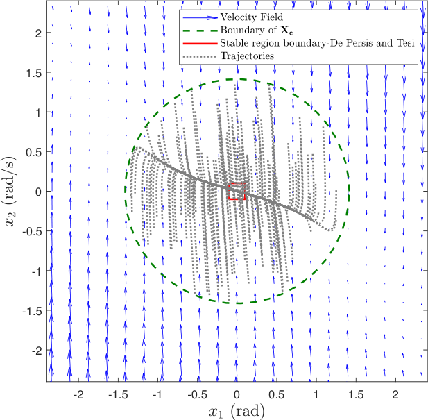
Fig. 2: Simulation results of the closed-loop system (33) with 𝐊=[−13.4283−13.5242]\mbf{K}=\begin{bmatrix}-13.4283&-13.5242\end{bmatrix}.

Example-2: Consider the inverted pendulum example in [13, Section V.B] in continuous time with the same unstable equilibrium at (𝐱𝟎,𝐮𝟎)=(𝟎,𝟎)(\mbf{x}_{0},u_{0})=(\mbf{0},0), which corresponds to the pendulum in upright position. The governing system is expressed in the closed-loop form as

δ​𝐱˙=([01g−μ]+𝟏𝟐𝟐​𝐊)​δ​𝐱+[𝟎𝐠𝐥​(sin⁡(δ​𝐱𝟏)−δ​𝐱𝟏)],\delta\dot{\mbf{x}}=\left(\begin{bmatrix}0&1\\ g&-\mu\end{bmatrix}+\mbf{1}_{2_{2}}\mbf{K}\right)\delta\mbf{x}+\begin{bmatrix}0\\ \frac{g}{l}(\sin{(\delta x_{1})}-\delta x_{1})\end{bmatrix},

(33)

where l=1l=1, g=9.8g=9.8, and μ=0.01\mu=0.01 (as in [13]). In this example, 𝐁𝟐=𝟏𝟐𝟐\mbf{B}_{2}=\mbf{1}_{2_{2}}, 𝐂𝟏=[𝟏𝟑𝟏𝟎]\mbf{C}_{1}=\begin{bmatrix}\mbf{1}_{3_{1}}&\mbf{0}\end{bmatrix} and 𝐃𝟏=𝟎\mbf{D}_{1}=\mbf{0}. Since the nonlinearity is independent of δ​u\delta u, we do not necessarily need to constrain the control input. However, performing the iterations in Algorithm 1 to reduce σ¯​(𝐊𝐖)\bar{\sigma}(\mbf{KW}) in turn reduces the control effort required, and we let these iterations continue for nmax=20n_{\text{max}}=20. In this setup, the maximum certified radius is α=2\alpha=\sqrt{2}, along with the controller 𝐊=[−13.4283−13.5242]\mbf{K}=\begin{bmatrix}-13.4283&-13.5242\end{bmatrix}. This controller is therefore able to drive the pendulum to its upright position from an initial displacement of approximately 81 degrees. The simulation results of the system (33) with this controller are depicted in Fig. 2 where, similar to Example-1, the vector field indicates that the closed-loop system can be driven to the equilibrium from a much larger region than the certified region 𝕏c\mathbb{X}_{c}. Indeed, there appears to be a stable manifold with the vector field converging to it (see Fig. 2). Also in Fig. 2, the red square denotes the local region certified in [13]. In comparison, the proposed controller is able to certify a much larger region. This improvement was achieved, in part, by utilizing the knowledge of the nominal LTI system whereas, the controller in [13] is purely data-driven. This example thus demonstrates the efficacy of the proposed method over a purely data-driven framework, given the nominal LTI system is known.

V Conclusions and Future Work

We presented an iterative method of local stabilization for nonlinear systems using sampled I/O data. Our approach uses I/O data to derive local norm bounds and synthesizes a robust state-feedback controller that is guaranteed to stabilize the system within the sampling region for the set of nonlinearities satisfying the norm bounds. The iterative steps require solving SDPs which can be done efficiently using freely available solvers. One of the numerical examples highlighted the reduced conservatism in our proposed synthesis method compared to a purely data-driven approach. Our future efforts will involve introducing parametric uncertainties and exogenous signals into the proposed framework. Also, we will investigate other ways to characterize I/O behavior of the nonlinearities (e.g., weighted 2-norm bounds) and extend our formulation to the output-feedback case.

References

  • [1] H. K. Khalil, Nonlinear Systems, 3rd ed. Upper Saddle River, NJ: Prentice Hall, 2002.
  • [2] J. Buch and P. Seiler, “Finite horizon robust synthesis using integral quadratic constraints,” Int. J. Robust Nonlin., vol. 31, no. 8, pp. 3011–3035, 2021.
  • [3] K.-C. Goh, M. Safonov, and J. Ly, “Robust synthesis via bilinear matrix inequalities,” Int. J. Robust Nonlin., vol. 6, no. 9-10, pp. 1079–1095, 1996.
  • [4] G. E. Dullerud and F. Paganini, A Course in Robust Control Theory: A Convex Approach. Springer Science & Business Media, 2000.
  • [5] A. Megretski and A. Rantzer, “System analysis via integral quadratic constraints,” IEEE T. Automat. Contr., vol. 42, no. 6, pp. 819–830, 1997.
  • [6] A. Packard and J. Doyle, “The complex structured singular value,” Automatica, vol. 29, no. 1, pp. 71–109, 1993.
  • [7] Z.-S. Hou and Z. Wang, “From model-based control to data-driven control: Survey, classification and perspective,” Information Sciences, vol. 235, pp. 3–35, 2013.
  • [8] A. Romer, J. Berberich, J. Köhler, and F. Allgöwer, “One-shot verification of dissipativity properties from input–output data,” IEEE Contr. Syst. L., vol. 3, no. 3, pp. 709–714, 2019.
  • [9] M. Tanemura and S.-i. Azuma, “Efficient data-driven estimation of passivity properties,” IEEE Contr. Syst. L., vol. 3, no. 2, pp. 398–403, 2018.
  • [10] J. Berberich, A. Koch, C. W. Scherer, and F. Allgöwer, “Robust data-driven state-feedback design,” in Amer. Contr. Conf., 2020, pp. 1532–1538.
  • [11] J. Na, J. Zhao, G. Gao, and Z. Li, “Output-feedback robust control of uncertain systems via online data-driven learning,” IEEE T. Neur. Net. Lear., vol. 32, no. 6, pp. 2650–2662, 2020.
  • [12] D. Wang, D. Liu, and H. Li, “Policy iteration algorithm for online design of robust control for a class of continuous-time nonlinear systems,” IEEE T. Autom. Sci. Eng., vol. 11, no. 2, pp. 627–632, 2014.
  • [13] C. De Persis and P. Tesi, “Formulas for data-driven control: Stabilization, optimality, and robustness,” IEEE T. Automat. Contr., vol. 65, no. 3, pp. 909–924, 2020.
  • [14] M. Tanaskovic, L. Fagiano, C. Novara, and M. Morari, “Data-driven control of nonlinear systems: An on-line direct approach,” Automatica, vol. 75, pp. 1–10, 2017.
  • [15] R. J. Caverly and J. R. Forbes, “LMI properties and applications in systems, stability, and control theory,” arXiv preprint arXiv:1903.08599, 2019.
  • [16] E. Warner and J. Scruggs, “Iterative convex overbounding algorithms for BMI optimization problems,” IFAC PapersOnLine, vol. 50, no. 1, pp. 10 449–10 455, 2017.
  • [17] J. Lofberg, “YALMIP: A toolbox for modeling and optimization in MATLAB,” in IEEE Int. Conf. Robot., 2004, pp. 284–289.
  • [18] M. ApS, The MOSEK optimization toolbox for MATLAB manual. Version 9.0., 2019.