A new method to invert InSAR data to resolve stress changes on a fracture embedded in a 3D heterogeneous crust

From a mathematical point of view, a volcano is a bounded open set $\Omega\subset\,\mathbb{R}^{3}$, occupied by an elastic solid. This set is assumed to have a smooth boundary $\partial\Omega$ which we separate in two (non empty) parts $\partial\Omega:={\Gamma_{\text{D}}}\cup\overline{\Gamma_{\text{N}}}$, with ${\Gamma_{\text{D}}}\cap{\Gamma_{\text{N}}}=\emptyset$. As depicted on Figure 1, the subset $\Gamma_{\text{N}}$ is actually the ground of the volcano and free to move. The subset $\Gamma_{\text{D}}$ is an artificial boundary defined in order to work on a finite size object and is assumed to to satisfy a 0 displacement condition. We assume that the elastic solid occupying $\Omega$ is subject to a body force field $\mathbf{f}$. In the sequel, boldface letters will be used to denote (usually $3$-dimensional) vector fields. Plain letters will represent scalar quantities.

We denote by $\mathbf{x}=(x,y,z)$ the generic point in $\,\mathbb{R}^{3}$, and by $\mathbf{u}=\mathbf{u}(\mathbf{x})$ the displacement field of the solid $\Omega$. The Cauchy stress $\sigma(\mathbf{u})$ and strain $\varepsilon(\mathbf{u})$ are given by

where $(\lambda,\mu)$ are the Lamé coefficients of the material, $\mathbf{I}_{\mathbb{R}^{3}}$ the identity matrix, and $\textrm{Tr}(\cdot)$ the matrix trace.

We also assume the presence of a crack in the volcano, which is represented mathematically by a 2-D surface $\Gamma_{\text{C}}\subset\Omega$ on which a traction or pressure force will be exerted (see also Figure 1). In a volcanic context, $\Gamma_{\text{C}}$ might represent a magma–filled crack on a fault. As already said in the introduction, the shape and position of the crack are supposed to be known in this work. The deformation field $\mathbf{u}$ of the solid is supposed to satisfy the following elastostatic system:

The first equation is the equilibrium law describing the (linear) elastic behaviour of the material. Condition (2) describes the fact that the displacement vanishes on the underground boundary of the solid. In equation (3), and in the sequel, ${\mathbf{n}}$ denotes the unit normal vector on the boundary of $\Omega$, oriented externally. This condition describes the free movement of the ground part of the volcano. Finally, equation (4) describes the force acting on the crack $\Gamma_{\text{C}}$. The vectors ${\mathbf{n}}^{+}$ and ${\mathbf{n}}^{-}=-{\mathbf{n}}^{+}$ are unit normal vectors on the crack $\Gamma_{\text{C}}$ (see Figure 2). The vector functions ${\mathbf{t}}^{\pm}(\mathbf{x})$ denote the force exerted on the crack. They are such that ${\mathbf{t}}^{+}=-{\mathbf{t}}^{-}$. When this force acts normally to the crack, that is ${\mathbf{t}}^{\pm}(\mathbf{x})=p(\mathbf{x}){\mathbf{n}}^{\pm}$, the force is called a pressure, otherwise in general it is called a traction force.

This traction force is the actual unknown of our problem. From the mathematical point of view it is supposed to be quadratically integrable as well as its gradient.

In order to derive a finite element approximation of the state equations (1)–(4), we need a weak formulation of the system. This is done by multiplying the equation (1) by a regular vector field ${\bf v}$ such that ${\bf v}=0$, and then integrating by parts over $\Omega$. Using the conditions (2)–(4) then yields:

where $:$ is the double inner product for matrices, i.e. for $A=(a_{ij})_{i,j=1,2,3}$ and $B=(b_{ij})_{i,j=1,2,3}$,

Notice that this approach allow us to deal with situations where the elastic material is nonhomogeneous and anisotropic, that is when the Lamé coefficients are not constant.

The direct problem (1)–(4) efficiently will have to be solved iteratively during the inversion procedure. Therefore we need an efficient algorithm to do so. To this aim, we use a domain decomposition method. More precisely, following [3], the domain $\Omega$ is split into two sub-domains such that each point of the domain lies on one side of the crack or on the crack. For this purpose, we use an artificial extension $\Gamma_{0}$ of the crack $\Gamma_{\text{C}}$. Assuming that $\Gamma_{\text{F}}=\Gamma_{\text{C}}\cup\Gamma_{0}$ splits the domain into two subdomains $\Omega^{+}$ and $\Omega^{-}$, we have $\Omega=\Omega^{+}\cup\Gamma_{\text{F}}\cup\Omega^{-}$, $\Gamma_{\text{N}}=\Gamma_{\text{N}}^{+}\cup\Gamma_{\text{N}}^{-}$ and $\Gamma_{\text{D}}=\Gamma_{\text{D}}^{+}\cup\Gamma_{\text{D}}^{-}$. We define on $\Gamma_{\text{C}}$ two opposite unit outward normal vectors ${\mathbf{n}}^{+}$ (from $\Omega^{+}$) and ${\mathbf{n}}^{-}$ (from $\Omega^{-}$). The global unknown ${\bf u}$ is split into ${\bf u}^{+}={\bf u}_{\mid\Omega^{+}}$ and ${\bf u}^{-}={\bf u}_{\mid\Omega^{-}}$.

Therefore, the equations (1)–(4) can be rewritten with ${\bf u}^{+}$ and ${\bf u}^{-}$ as unknowns:

where $[\![{\bf v}]\!]={\bf v}^{+}-{\bf v}^{-}$ denotes the jump of a function across $\Gamma_{0}$. The equations and conditions (6)–(9) are a straightforward rewriting of (1)–(4). The two last conditions (10) and (11) are imposed to enforce the continuity of displacement and stress across $\Gamma_{0}$ to ensure that ${\bf u}=({\bf u}^{-},{\bf u}^{+})$ solves the original problem (1)–(4).

Let us now describe the discretization of this problem via the finite element method. A lagrange multiplier $\lambda$ defined on $\Gamma_{0}$ is introduced to enforce the continuity of the displacement across the $\Gamma_{0}$. Defining the associated lagrangian functional and expressing the associated saddle point conditions give a weak formulation for Problem (6)–(11) which unknown is in the form ${\bf X}=({\bf u}^{+},{\bf u}^{-},\boldsymbol{\lambda})^{\top}$ (see [3] for details).

In order to numerically approximate the system, consider a tetrahedral mesh of $\Omega$ (as e.g. in Figure 3). Let $\boldsymbol{\varphi}^{\pm}_{i}$ be a finite element basis defined on this mesh. Also defining a mesh of the extended crack, we build finite elements bases $\boldsymbol{\psi}_{i}$ and $\boldsymbol{\theta}_{j}$ on $\Gamma_{0}$ and $\Gamma_{\text{C}}$ respectively.

Identifying the unknowns ${\bf u}^{+}$, ${\bf u}^{-}$ and $\boldsymbol{\lambda}$ with there value on the nodes of the mesh, the discretized form of Problem (6)–(11), then reads

The matrix $\mathrm{K}$ of this system is built from the stiffness matrices $A^{\pm}$, and the constraint coupling matrices on $\Gamma_{0}$ denoted by $B^{\pm}$. More precisely, we have

where

The right hand side vector ${\bf F}^{\pm}$ is given by

which boils down to the algebraic formulation

where the mass matrices $M_{\Omega}^{\pm}$ and the coupling matrix on $\Gamma_{\text{C}}$, denoted by $M_{C}$, are given by

Eventually, we can naturally define two matrices $L_{\Omega}$ and $L_{C}$ such that we have

The matrix $K$ is symmetric and positive definite, which allows the use of powerful classical solvers. The implementation of this model uses the finite element library GetFem++ [9]. The library provides all the necessary tools to handle various types of PDEs, and links to classical powerful solvers (conjugate gradient, SuperLU, MUMPS) as well as other routines for mesh management, definition of cracks and boundaries via level set functions) which make it quite versatile and powerful. We refer the reader to [3] for a detailed mathematical and computational analysis of this method. See also [1, 2] for a mathematical analysis of similar optimal control problems aking use of the domains decomposition technique.

Let us assume the displacement field of the volcano to be fully measured on the ground $\Gamma_{\text{N}}$, and call it $\mathbf{u}_{d}$. The inversion problem consists in finding a traction vector ${\mathbf{t}}$ such that the solution of Problem (1)–(4) satisfies $\mathbf{u}=\mathbf{u}_{d}$ on $\Gamma_{\text{N}}$. However this is known to be an ill-posed problem (e.g. the solution is not unique), and moreover the measurements are perturbed by random uncertainties. Therefore we adopt a least squares approach, combined with a regularization (i.e. smoothing) technique to build the inversion process.

Consider the following cost function:

where ${\mathbf{C}}$ denotes the covariance operator of the measurements uncertainties (see e.g. [11]), and is assumed to be positive definite, $\top$ denotes the transpose operator, and finally, the non–negative constants $\alpha_{0}$ and $\alpha_{1}$ are the Tikhonov regularization (or smoothing) parameters.

We aim at minimizing this cost function over the space of feasible traction vectors. This space consists in quadratically integrable vectors, which gradient is also quadratically integrable.

In [1, 2], a simplified version of this problem is mathematically studied. The cost function only features the first smoothing term. As it will be shown later on, our tests have proved the necessity of smoothing the gradient, in a practical framework, to obtain a physically admissible solution ${\mathbf{t}}$. The optimal choices for the values of $\alpha_{0}$ and $\alpha_{1}$ will be discussed further.

To derive the optimality conditions for the Problem (13), we introduce the following Lagrangian:

where $\boldsymbol{\phi}$ is the Lagrange multiplier for the constraint (1)–(4) in the weak form (5). When $\nabla_{{\bf u}}{\mathcal{L}}=0$ and $\nabla_{\boldsymbol{\phi}}{\mathcal{L}}=0$, we have $\nabla_{{\mathbf{t}}}{\mathcal{L}}=\nabla J$. Cancelling $\nabla_{\boldsymbol{\phi}}{\mathcal{L}}$ gives problem (1)–(4). Cancelling $\nabla_{{\bf u}}{\mathcal{L}}$ and performing integration by parts yields that $\boldsymbol{\phi}$ is the solution of

called the adjoint state system. Finally, computing $\nabla_{{\bf u}}{\mathcal{L}}$, for ${\bf u}$ and $\boldsymbol{\phi}$ satisfying (1)–(4) and (14), gives:

We refer the reader to [1, 2], for further details.

After splitting the computational domain $\Omega$, the cost function $J$ in the optimization problem (13) becomes:

The previous optimality conditions rewrite naturally from this new formulation.

The next step is to adapt the cost function, the adjoint state and the gradient of the cost function to the discrete system (12). To this aim, it has to be noticed that all terms in (16) are symmetric. Discretizing the two first terms will involve the introduction of mass matrices on $\Gamma_{\text{N}}^{\pm}$. On needs to keep the symmetry of the discrete form. Since the covariance matrix $\mathbf{C}$ is positive definite, it is also the same for its inverse and we can write

where $Q$ is the matrix which columns are the eigenvectors of $\mathbf{C}$ and $D$ the diagonal matrix of the eigenvalues of $\mathbf{C}$. This diagonalized form allows us to write $\mathbf{C}^{-1}=\mathbf{C}^{-\frac{1}{2}}\mathbf{C}^{-\frac{1}{2}}$, where

In view of this, we rewrite the continuous cost function $J$ as

As in Section 1.2, we will identify the previous functions with their values at the mesh nodes. Define a set of finite element basis functions $\boldsymbol{\chi}_{i}^{\pm}$ (with 3 degrees of freedom at each mesh node) defined on $\Gamma_{\text{N}}^{\pm}$. Then, define the ground mass matrix

with $\displaystyle\left[M_{G}^{\pm}\right]_{ij}=\int_{\Gamma_{\text{N}}}\boldsymbol{\chi}_{i}^{\pm}\cdot\boldsymbol{\chi}_{j}^{\pm}\,\mathrm{d}\Gamma_{\text{N}}$. Let us also define the matrices $M_{F_{0}}$ and $M_{F_{1}}$ as

Recall that $\boldsymbol{\theta}_{j}$ are the finite element basis functions defined on $\Gamma_{\text{C}}$.

Finally, in view of the domain decomposition method, the mesh nodes located on the ground will be on either side of the crack. Therefore, the measured displacement and the restriction to the ground nodes of the computed displacement (denoted ${\bf u}_{G}$) can be written as

Consider then the reduction matrix $\mathcal{O}_{R}$ such that

where ${\bf X}$ is the solution of (12).

The discrete version of the cost function $J$ defined by (17) is then

The optimality conditions for the minimizer of the discrete cost function $J_{\mathtt{d}}$ are obtained via the characterization of the saddle point of the following (discrete) Lagrangian function:

Computing the partial derivative of ${\mathcal{L}}_{\mathtt{d}}$ and then cancelling them, lead to the discrete counterpart of the adjoint problem (14) as:

which rewrites, denoting ${\bf u}_{G}=\mathcal{O}_{R}{\bf X}$,

where $K$ is the (symmetric) matrix of System (12). The gradient of $J_{\mathtt{d}}$ at any point ${\mathbf{t}}$ is then:

In a previous work (see [2]), we presented two methods to minimize a simpler version of our cost function $J_{\mathtt{d}}$ : the conjugate gradient algorithm and a quasi-Newton method (low storage BFGS). These two techniques are natural choices due to the quadratic structure of the cost function. They were studied in depth in terms of computational performance and accuracy. The BFGS method appeared to be converging faster when the mesh of the domain $\Omega$ is rather coarse. When the mesh becomes finer, the number of unknowns in the problem increases and the two methods tend to give similar results. In the framework of applications which we are interested in, we aim at fast processes, that is we will most of the time consider meshes that are rather coarse except in the neighborhood of the crack $\Gamma_{\text{C}}$. Therefore we will use a BFGS algorithm (see [4, 5, 7, 10]) in our numerical tests. It involves the construction of a sequence of approximation of the inverse of the Hessian matrix of the cost function $J_{\mathtt{d}}$. We use a limited storage version of the algorithm called L-BFGS (see [8]). The method is presented in Algorithm 1, with the necessary adaptations to our problem.

As usual with this type of methods sequences are built and will be denoted as follows:

• •

  ${\mathbf{t}}^{k}$: traction force vector,

• •

  ${\bf X}^{k}$: solution of the state equation (12),

• •

  ${\bf u}^{k}$ : displacement field on the ground,

• •

  $\phi^{k}$: solution of the adjoint state equation (20),

• •

  ${\mathbf{g}}^{k}$: gradient of the cost function $J_{\mathtt{d}}$ at point ${\mathbf{t}}^{k}$,

• •

  ${\mathbf{d}}^{k},\mathbf{w}^{k}$: displacement directions for the optimization,

• •

  $\rho^{k}$: optimal displacement step.

The number $k\geq 0$ represents the iteration number.

Notice that the underlying quadratic form in the cost function allow to compute explicitely the optimal step size at each iteration, via formula (28). The detailed computation is presented in the Appendix.

In the algorithm, the domain decomposition technique is used to solve the discrete state and adjoint state equations (12) and (20). Notice that the matrix $K$ is symmetric and does not change during the iterative process, which means that the computation cost due to matrix factorization is reduced.

The algorithm iterates until the gradient of $J_{\mathtt{d}}$ becomes sufficiently small, as precised in the algorithm below.

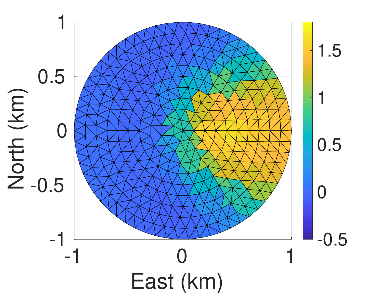
The numerical application is performed by a synthetic test via simulation of a flat volcano as follows: A semi-infinite elastic domain at center with radius $100$ km and extending down to $[0,−20]$ km (see Figure 3(a)), with the elasticity parameters: the Young modulus $E=5000.0$ MPa and Poisson ratio $\nu=0.25$. A horizontal circular fracture is defined with radius $r=1$ km and located at $(x,y,z)=(0,0,−0.3)$ km in the topo flat. The mesh generation and level set implementation is explained in [1, 2]. The ground surface is free to move and the other sides is fixed i.e. satisfy the boundary conditions on $\Gamma_{\text{N}}$ and $\Gamma_{\text{D}}$ respectively. We generated a synthetic solution ${\bf u}_{d}$ associated to a discontinuous traction ${\mathbf{t}}^{\pm}=(0,0,\pm 1.5)$ MPa, applied on a part of the fracture $\Gamma_{\text{C}}$, as shown in Figure 3(b) (the yellow patches) and ${\mathbf{t}}^{\pm}=(0,0,0)$ on the rest of the fracture (the blue patches). In some numerical experiments, this traction is interpreted as a pressure ${\bf p}^{\pm}=1.5$ MPa applied on the yellow zone.

Finding a robust and efficient method to compute appropriate regularization parameters $\alpha_{0}$ and $\alpha_{1}$ for given mesh and noisy data, is not straightforward. The admissible solution ${\mathbf{t}}$ is dependent on the chosen $\alpha_{0}$ and $\alpha_{1}$ and it is crucial to obtain a good approximation of the solution to the optimization problem. For choosing the optimal parameters, a series of tests is organized by using the graphical tools. Indeed, three important criteria are compared by varying $\alpha_{0}$ and $\alpha_{1}$ as follows: we set $\alpha_{0}\in\{1.0\mathrm{E}-12,1.0\mathrm{E}-11,\ldots,1.0\mathrm{E}0\}$ and $\alpha_{1}\in\{1.0\mathrm{E}-5,1.0\mathrm{E}-4,\ldots,1.0\mathrm{E}5\}$. Then we compare: A relative ground error defined by:

A relative error of traction ${\mathbf{t}}$ on the fracture source, defined by:

Note that an inevitable numerical error is already produced to compute the traction ${\mathbf{t}}$ on the fracture source. Using the non-conformal mesh to implement the fracture by level set method, is the reason of this error which can be reduced by using a finer mesh around the fracture.
finally, the iteration number for a given $\epsilon=1.0\mathrm{E}-14$ in Algorithm 1 to satisfying the convergence criteria

The numerical tests presented in Figure 4, show that, $\alpha_{1}=1$ can be chosen as an acceptable parameter. Moreover, it seems, the above criteria are less sensitive to $\alpha_{0}$ between $1.0\mathrm{E}-7$ and $1.0\mathrm{E}-4$. Accordingly, we employ L-curve, another graphical tool, to trade off between two criteria: the misfit

and the norm of the traction or smoothing

The L-curves are depicted by setting $\alpha_{0}=1.0\mathrm{E}-7$ and varying $\alpha_{1}$. Closest point to the origin shows the best compromise between misfit and smoothing, and it will be the acceptable $\alpha_{1}$. In particular case when we aim to find the pressure, the traction ${\mathbf{t}}$ may replaced by the pressure ${\bf p}$. In Figure 5, for the above fracture and mesh, two L-curves corresponding to both pressure ${\bf p}$ and traction ${\mathbf{t}}$ are illustrated.

Fracture pressure corresponding to $\alpha_{1}=1.0\mathrm{E}1$ as an appropriate choice is presented in Figure 5(c). As shown in Figures 6 and 7, in 3D realistic volcanoes where we interested in large-scale problem, the values around the $1.0\mathrm{E}1$ are yet acceptable. Normal and tangential tractions are depicted in Figure 7. Note that we suppose $(0,0,-1)$ as the unit normal vector ${\mathbf{n}}$.

We then aim to consider the impact of the fracture depth to the approximated admissible solution. To do that, the numerical experiments are repeated for the fracture at $-0.9$ km of depth. The best combination for $\alpha_{1}=1.0\mathrm{E}-1$ and $\alpha_{0}$ between $1.0\mathrm{E}-7$ and $1.0\mathrm{E}-4$, in red box are shown in Figure 8. The L-curves depicted for ${\bf p}$ and ${\mathbf{t}}$ in Figure 9(a, b) show that the closest point to the origin for the $0.9$ km is $\alpha_{1}=1.0\mathrm{E}0$. The normal stress projected on the fracture presented in Figure 9(c) compare to exact solution confirms an acceptable approximated solution. As previous case the values around the $1.0\mathrm{E}0$ for $\alpha_{1}$ are acceptable (see Figures 12 and 13). A comparison of the iteration number presented in Table 1, indicates that the number of iterations is augmented for the greater values of $\alpha_{1}$.

As seen in the numerical simulations, we may trust to the L-curves results to find an appropriate $\alpha_{1}$ for more complicated geometry of fracture and mesh, which is clearly help us to computational cost.

Before going further, let us first remark that the previous section can easily be adapted to the case where the measurements of the displacement field are performed only on a part of the ground $\widetilde{\Gamma_{\text{N}}}\subset\Gamma_{\text{N}}$. The cost function to be minimized becomes

Rewriting the optimality conditions and adapting the algorithms is straightforward. This is what is actually implemented in our software.

However, assuming the displacement field to be known in cartesian coordinates is not realistic for the applications. In this section we aim at adapting our work to the case where measurements are provides by satellite radar interferometry (as e.g. in[6]). We will first state precisely what measurements are made and then adapt our methods to this new framework.

Let $\mathbf{u}_{d}=(u_{x},u_{y},u_{z})^{\top}$ be a displacement field on $\Gamma_{\text{N}}$, written in cartesian coordinates. A satellite will aim at the ground to measure a displacement, and the resulting measurement will be in the form ${\bf p}^{\top}\mathbf{u}_{d}$ where the aiming direction (also called earth-satellite direction) ${\bf p}=(p_{x},p_{y},p_{z})$ is a unit vector oriented from the ground to the satellite. Let then $N\geq 1$ be the number of satellites, each associated to a direction ${\bf p}_{i}=(p_{ix},p_{iy},p_{iz})$ for $i=1,\ldots,N$. We can build a matrix $\mathbf{P}:\mathbb{R}^{3}\rightarrow\mathbb{R}^{N}$ as $\mathbf{P}=({\bf p}_{1},{\bf p}_{2},\cdots,{\bf p}_{N})^{\top}$, so that the actual measurement is

The vector field $\mathbf{R}_{d}\in\mathbb{R}^{N}$ is defined on $\Gamma_{\text{N}}$, and the matrix $\mathbf{P}$ also operates on the solutions of System (1)–(4). Hence, given the field $\mathbf{R}_{d}$, our new optimization problem consists now in finding the traction vector ${\mathbf{t}}$ minimizing the following cost function:

where $\alpha_{0}>0$ and $\alpha_{1}>0$ are the regularization parameters. The optimality conditions for this problem are derived in the same way than in Section 2.1. We will not go into details about this and focus on the discrete version of the problem.

Using the definitions of Sections 1.2 and 2.2, and in view of (19) and (24) the discrete cost function becomes

where $X$ is the solution of the discrete system (12). This finite dimensional problem then boils down to finding the saddle point of the following Lagrangian

Computing the partial derivative of ${\mathcal{L}}_{\mathtt{d}}$ and then cancelling them, leads to the discrete adjoint problem (14):

and the gradient of $J_{\mathtt{d}}$ is:

The minimization Algorithm 1 can then be adapted to the new adjoint state and gradient to obtain the numerical approximation of the traction ${\mathbf{t}}$ on the crack by using the surface measurements provided by radar interferometry $\mathbf{r}_{d}$.

The numerical applications here are proceeded in three different steps: First, we aim to the adaptation of the theoretical results in Earth-Satellite directions. For the sake of simplicity, we assume the covariance is an identity matrix. Next, in order to reduce the observed data, the identity covariance matrix is reduced to the nodal mesh points. We then consider a problem with dense covariance matrix adapted to a limited number of observed data.

The vector directions are chosen by using InSAR satellite directions, listed in Table 2. The numerical tests are performed with one to four radar looks to confirm the theoretical results. We set the same configuration as previous section for the problems in Cartesian coordinate. The horizontal circular fracture beneath the flat topography located at $0.3$ km (see Figure 3). We still take $\alpha_{0}=10^{-7}$ and by depicting the L-curves, we find the best $\alpha_{1}$ with the best compromise between misfit and the traction norm ${\mathbf{t}}$ or pressure ${\bf p}$ (see Figure 10) Normal and tangential tractions projected on the fracture corresponding to the best $\alpha_{1}=1$ are presented in Section supplementary Material, Figure 14. A comparison between the iteration numbers listed in Table 3 for the observed synthetic data provided by different number of radar looks, show that the use of more radar looks leads to a decrease in the number of iteration.

In a more realistic scenario, the number of observed data are limited. In the previous numerical experiments, we assumed a synthetic ${\bf u}_{d}$ in $\text{P}2$ finite elements. The degrees of freedom’s nodes of a classical $\text{P}2$ Lagrange elements on a 3D tetrahedron, are located on the vertices or nodal mesh points and the midpoints of the edges. In realistic volcano phenomenons (three-dimensional elasticity problem), using the $\text{P}2$ finite element guarantees a good approximated solution. However, we aim to reduce the synthetic ${\bf u}_{d}$ to nodal mesh points on the ground surface as a $\text{P}1$ finite elements. On the other side, to conserve the $\text{P}2$ finite elements for the elasticity problem, we should conserve the dimension of the covariance $\mathbf{C}^{-\frac{1}{2}}$ and the mass matrix $M_{G}$ in a $\text{P}2$ elements. Therefore, from implementation point of view, the degrees of freedom’s related to the midpoints of the edges in $\mathbf{C}^{-\frac{1}{2}}$ and $M_{G}$ are set to zero. Despite the increase in the iterations number, the numerical experiments presented still show very satisfactory results (see Section Supplementary Material Figure 15).

Another step to approach the reality is using the dense covariance matrices for limited number of data, obtained by InSAR and cGNSS.

To do that, we are using the DEfvolc interfaces The dense covariance matrices are provided by DefVolc, pre and post-processor software. We started by creating the synthetic ${\bf u}_{d}$ and the dense covariance matrix in S4 radar look. The results obtained in Figure 11 and first row of Table 4, confirm the adaptability of our method to the dense covariance matrices. In reality, most of the time, the atmospheric contribution caused masked and noisy InSAR data. Therefore, some numerical experiments is performed by creating masked and noisy synthetic ${\bf u}_{d}$ and covariance matrix. The numerical experiments are presented in Figure 11. The L-curves are depicted for synthetic ${\bf u}_{d}$ projected to S4 an S6 directions. First without any mask and noise in the data and then different possible cases by adding the mask and noise to the synthetic data. We summarized appropriate choices for $\alpha_{1}$ and the number of iterations to achieve the convergence with these $\alpha_{1}$, for different cases of synthetic ${\bf u}_{d}$, in Table 4. Despite of choosing a greater $\alpha_{1}$, for the masked data, the number of iteration is reduced. However, for the noisy data the convergence of the inversion process is much more harder. Moreover the vector size of the synthetic ${\bf u}_{d}$ for each case are listed in Table 4.

This section is dedicated to some mathematical details for interested readers. First part is concerned to compute the optimal step size. To simplify the presentation, let us introduce $c_{N}$ defined on $\Gamma_{\text{C}}$

so that the cost functional in (13) becomes

Then the directional derivative of $J$ in the direction of a given ${\mathbf{d}}$ reads

where $\mathbf{w}$ is the solution to (5) with ${\mathbf{t}}={\mathbf{d}}$. Therefore, we may compute the optimal step size $\rho$, with a search direction $d$ by solving

that is

which gives

The optimal step size is therefore

The second part is concerned to L-BFGS Update in minimization Algorithm 1

References

• [1] O. Bodart, V. Cayol, F. Dabaghi, and J. Koko. Fictitious domain method for an inverse problem in volcanoes. Springer, Domain Decomposition Methods in Science and Engineering XXV. DD 2018. Lecture Notes in Computational Science and Engineering, 138, 2020.
• [2] Oliver Bodart, Valérie Cayol, Farshid Dabaghi, and Jonas Koko. An inverse problem in an elastic domain with a crack : a fictitious domain approach. submitted, 2021.
• [3] Olivier Bodart, Valérie Cayol, Sébastien Court, and Jonas Koko. Xfem-based fictitious domain method for linear elasticity model with crack. SIAM Journal on Scientific Computing, 38(2):B219–B246, 2016.
• [4] C. G. BROYDEN. The convergence of a class of double-rank minimization algorithms 1. general considerations. IMA Journal of Applied Mathematics, 6(1):76–90, 1970.
• [5] R. Fletcher. A new approach to variable metric algorithms. The Computer Journal, 13(3):317–322, 1970.
• [6] Y. Fukushima, V. Cayol, and P. Durand. Finding realistic dike models from interferometric synthetic aperture radar data: The february 2000 eruption at piton de la fournaise. Journal of Geophysical Research: Solid Earth, 110(B3).
• [7] Donald Goldfarb. A family of variable-metric methods derived by variational means. Math. Comp., 24:23–26, 1970.
• [8] Jorge Nocedal. Updating quasi-newton matrices with limited storage. Mathematics of Computation, 35(151):773–782, 1980.
• [9] Y. Renard and J. Pommier. Getfem++. An Open Source generic C++ library for finite element methods. http://home.gna.org/getfem.
• [10] D. F. Shanno. Conditioning of quasi-newton methods for function minimization. Math. Comp., 24:647–656, 1970.
• [11] A. Tarantola. Inverse Problem Theory and Methods for Model Parameter Estimation. Society for Industrial and Applied Mathematics, 2005.