DiffTune+: Hyperparameter-Free Auto-Tuning using Auto-DifferentiationMechanical Science and Engineering, University of Illinois Urbana-Champaign, Urbana, IL 61801Computer Science, University of Illinois Urbana-Champaign, Urbana, IL 61801
Abstract
Controller tuning is a vital step to ensure the controller delivers its designed performance. DiffTune has been proposed as an automatic tuning method that unrolls the dynamical system and controller into a computational graph and uses auto-differentiation to obtain the gradient for the controller’s parameter update. However, DiffTune uses the vanilla gradient descent to iteratively update the parameter, in which the performance largely depends on the choice of the learning rate (as a hyperparameter). In this paper, we propose to use hyperparameter-free methods to update the controller parameters. We find the optimal parameter update by maximizing the loss reduction, where a predicted loss based on the approximated state and control is used for the maximization. Two methods are proposed to optimally update the parameters and are compared with related variants in simulations on a Dubin’s car and a quadrotor. Simulation experiments show that the proposed first-order method outperforms the hyperparameter-based methods and is more robust than the second-order hyperparameter-free methods.
keywords
Auto-tune, Controller tuning, Auto-Differentiation1 Introduction
Controller design and tuning are two vital steps in applying control techniques to a system: controller design roots in qualitative analysis to ensure stability, whereas parameter tuning delivers the desired performance on real systems. Controller tuning is normally done by hand, by either trial-and-error or proven methods for specific controllers (e.g., Ziegler–Nichols method for proportional-integral-derivative (PID) controller tuning (O’dwyer 2009)). However, hand-tuning often requires experienced personnel and can be inefficient, especially for systems with long loop times or huge parameter space.
To improve efficiency and performance, automatic tuning (or auto-tune) methods have been investigated. Such methods integrate system knowledge, expert experience, and software tools to determine the best set of controller parameters, especially for the widely used PID controllers (Yu 2006; Åström et al. 1993; Li et al. 2006). Commercial auto-tune products have been available since 1980s (Zhuang and Atherton 1993; Åström et al. 1993). Existing auto-tune methods can be categorized into model-based (Trimpe et al. 2014; Kumar and Ramadge 2021; Cheng et al. 2022a) and model-free (Marco et al. 2016; Berkenkamp et al. 2016; Calandra et al. 2014; Lizotte et al. 2007; Loquercio et al. 2022; Mehndiratta et al. 2021). Both approaches iteratively select the next set of parameters for evaluation that is likely to improve the performance of the previous trials. Model-based auto-tune methods leverage knowledge of the system model and apply gradient descent so that the performance can improve based on the local gradient information (Trimpe et al. 2014; Kumar and Ramadge 2021). Stability can be ensured by explicitly leveraging knowledge about the system dynamics. However, model-based auto-tune might not work in a real environment due to imperfect model knowledge. Model-free auto-tune methods rely on an approximated gradient or a surrogate model to improve the performance. Representative approaches include Markov chain Monte Carlo (Loquercio et al. 2022), Gaussian process (GP) (Marco et al. 2016; Berkenkamp et al. 2016; Calandra et al. 2014; Lizotte et al. 2007), and deep neural network (DNN) (Mehndiratta et al. 2021). Such approaches often make no assumptions on the model and are compatible with real data owing to their data-driven nature. However, some model-free approaches (e.g., GPs) are inefficient when tuning in high-dimensional parameter spaces. Besides, establishing stability guarantees with data-driven methods is hard, where empirical methods are often applied.
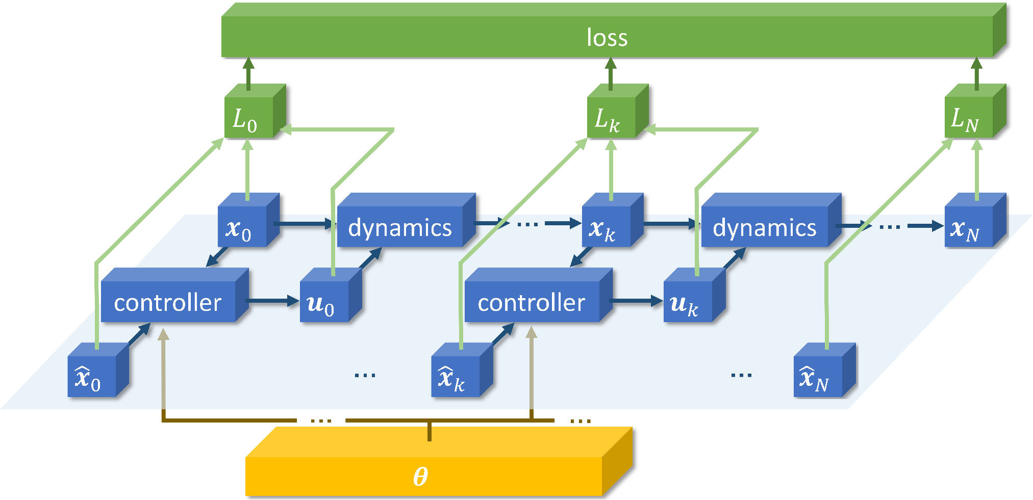
To overcome the challenges in the auto-tune scheme, DiffTune (Cheng et al. 2022a) has been proposed as a model-based auto-tune method based on auto-differentiation (AD). DiffTune unrolls a dynamical system into a computational graph, as shown in Figure 1. Based on the computational graph, DiffTune iteratively improves the system performance by tuning the controller parameters using the analytical gradient. When the computational graph is unbroken, both forward- and reverse-mode ADs can be applied to compute the analytical gradient. However, the computational graph is broken when incorporating real systems’ data because the new system states are obtained through sensor measurements or state estimation instead of evaluating those from the dynamics. The broken computational graph forbids the usage of forward- or reserve-mode AD. In this case, we propose the “sensitivity propagation,” which essentially propagates the sensitivity of an ordinary differential equation (ODE) system (Khalil 2015; Ma et al. 2021). The measured or estimated state information is applied to propagate the gradient in the forward direction in parallel to the dynamics’ propagation.
DiffTune enjoys three qualities for autotune schemes: stability is inherited from the controllers with stability guarantees by design; real-data compatibility is enabled by the sensitivity propagation; and efficiency is provided since the sensitivity propagation runs forward in time and in parallel to the system’s evolution. DiffTune is generally applicable to tune all the controller parameters as long as the system dynamics and controller are differentiable, which is the case with most of the systems. For example, algebraically computed controllers, e.g., with the structure of gain-times-error (PID (Kumar and Ramadge 2021)), are differentiable. Moreover, following the seminal work (Amos and Kolter 2017) that differentiates the argmin operator using the implicit differentiation, one can see that controllers relying on a solution of an optimization problem to generate control actions (Amos et al. 2018; East et al. 2020; Jin et al. 2020; Jin et al. 2022; Ma et al. 2022; Xiao et al. 2021; Xiao et al. 2022; Parwana and Panagou 2021; Vien and Neumann 2021) are readily differentiable.
Despite the merits of DiffTune stated above, what is still missing in DiffTune is the tuning efficiency: the original DiffTune framework (Cheng et al. 2022a) uses vanilla gradient descent to improve the performance iteratively. Such a first-order method is not efficient enough since the convergence speed largely depends on the learning rate, which needs to be tuned as a hyperparameter. This issue motivates us to look into hyperparameter-free approaches that choose the learning rate “optimally.” More generally, we study how the parameter can be updated “optimally.” We apply a first-order approximation of the closed-loop state trajectory using sensitivity, where the approximation essentially serves as the predicted state corresponding to updated parameters. The approximation leads to a predicted loss, analyzing which permits to derive the explicit formula for the optimal learning rate or, more generally, the optimal parameter update, which is hyperparameter-free. We implement the above-mentioned methods together with related first-order and second-order methods in simulations on a Dubin’s car model and a quadrotor model and compare their performance.
Our contributions are summarized as follows: i) We show deeper insights into DiffTune from the perspective of first-order approximation of the predicted state trajectory using sensitivity. These insights allow for predicting the loss change when the controller parameters change, which further enables optimal parameter updates subject to a certain criterion. ii) Based on the new insights, we improve DiffTune’s gradient descent method by proposing hyperparameter-free alternatives and compare their performance with related variants in simulations.
The remainder of the paper is organized as follows: Section 2 reviews the related work of this paper. Section 3 introduces the technical background and fundamentals of DiffTune. Section 4 describes the usage of sensitivity for predicting state trajectory subject to parameter change and derives optimal parameter updates (and their closely related variants). Section 5 shows the simulation results on a Dubins’ car and on a quadrotor. Finally, Section 6 concludes the paper.
2 Related Work
We briefly review previous work in the following four domains: automatic parameter tuning, learning-based controllers, recurrent neural networks (for the resemblance between their recurrent form and the iterative nature of dynamical systems), and second-order methods for unconstrained optimization.
Model-based auto-tune leverages model knowledge to infer the parameter choice for performance improvement. In (Trimpe et al. 2014), an auto-tune method is proposed for a linear quadratic regulator (LQR). The gradient of a loss function with respect to the parameterized quadratic matrix coefficients is approximated using Simultaneous Perturbation Stochastic Approximation (Spall 2005). In (Kumar and Ramadge 2021), the gradient of a quadratic loss over input control actions and system outputs with respect to PID gains is computed using auto-differentiation tools. In (Wiedemann et al. 2022), a controller is trained via analytical policy gradient, which achieves similar or better performance than model-based and model-free reinforcement learning (while requiring less training data) and similar performance to MPC (while reducing the computation time). In (Romero et al. 2022), the authors use a probabilistic policy search method (weighted maximum likelihood) to tune a model predictive contour controller for quadrotor agile flight.
Model-free auto-tune relies on a zeroth-order approximate gradient or surrogate performance model to decide the new candidate parameters. In (Killingsworth and Krstic 2006), the authors use extremum seeking to sinusoidally perturb the PID gains and then estimate the gradient. Gradient-free methods, e.g., Metropolis-Hastings sampling (Loquercio et al. 2022), have also been used for tuning. In terms of surrogate models, machine learning tools have been frequently used for their advantages in incorporating data. In (Edwards et al. 2021), an end-to-end, data-driven hyperparameter tuning is applied to an MPC using a surrogate dynamical model. Besides, GP is often used as a non-parametric model that approximates an unknown function from input-output pairs with probabilistic confidence measures. This property makes GP a suitable surrogate model that approximates the performance function with respect to the tunable parameters. In (Marco et al. 2016), GP is applied to approximate the unknown cost function using noisy evaluations and then induce the probability distribution of the parameters that minimize the loss. In (Berkenkamp et al. 2016), the authors use GP to approximate the cost map over controller parameters while constructing safe sets of parameters to ensure safe exploration. Similar ideas have been applied to gait optimization for bipedal walking, where GP is used to approximate the cost map of parameterized gaits (Calandra et al. 2014; Lizotte et al. 2007). Besides GP, deep neural networks (DNNs) (Mehndiratta et al. 2021) have also been used for model-free tuning.
Learning for control is a recently trending research direction that strives to combine the advantages of model-driven control and data-driven learning for the safe operation of a robotic system. Exemplary approaches include, but are not limited to, the following: reinforcement learning (Polydoros and Nalpantidis 2017; Tambon et al. 2022), whose goal is to find an optimal policy while gathering data and knowledge of the system dynamics from interactions with the system; imitation learning (Ravichandar et al. 2020), which aims to mimic the actions taken by a superior controller while making decisions using less information of the system than the superior controller; and iterative learning control (Xu 2011; Bristow et al. 2006), which constructs the present control action by exploiting every possibility to incorporate past control and system information, typically for systems working in a repetitive mode. A recent survey (Brunke et al. 2022) provides a thorough review of the safety aspect of learning for control in robotics.
Recurrent neural networks (RNNs) refer to the artificial neural networks that have recurrent connections. Recent advances in RNNs have been summarized in (Salehinejad et al. 2017). The recurrent structure of an RNN makes it resemble a discrete-time dynamical system: the gradient vanishing/exploding phenomenon when training an RNN using backpropagation through time (BPTT) can be explained using equilibrium and contracting region of an ODE (Bengio et al. 1994). A short review of the methods for handling the gradient vanishing/exploding issue is provided in (Salehinejad et al. 2017). The BPTT is closely related to the sensitivity analysis of an ODE system. A recent study (Ma et al. 2021) has shown that the discrete local sensitivity implemented via forward-mode AD is more efficient than reverse-mode AD and continuous forward/adjoint sensitivity analysis.
Second-order methods for unconstrained optimization use the Hessian matrix to scale the gradients with curvature information, which eliminates the need for hyperparameter tuning in the first-order methods to achieve satisfactory convergence. The most straightforward second-order method is the Newton method, where the inverse of the Hessian matrix scales the gradient using curvature. However, since inverting a Hessian matrix is computationally intensive, alternative methods like Quasi-Newton, Gauss-Newton, Levenberg-Marquardt, conjugate gradient methods (Nocedal and Wright 1999) are applied with various ways to approximate the inverse Hessian matrix. Notably, differentiable Gauss-Newton (Ma et al. 2019) and Levenberg-Marquardt (Tang and Tan 2018) have been proposed in recent years to enable end-to-end learning through these second-order methods.
3 Background
Consider a discrete-time dynamical system
| (1) |
where and are the state and control, respectively, and the initial state is known. The control is generated by a feedback controller that tracks the desired state such that
| (2) |
where denotes the parameters of the controller. The tuning task adjusts to minimize an evaluation criterion, denoted by , which is a function of the desired states, actual states, and control actions over a time interval of length .
DiffTune gradually improves the system performance by tuning the controller parameters using gradient descent. Specifically, since the controller is stable for within the feasible set , we use the projected gradient descent to update (Cheng et al. 2022a) (and ensure stability):
| (3) |
where is the projection operator (Parikh et al. 2014) that projects its operand into the set and is the step size. To obtain , DiffTune unrolls the dynamical system (1) and controller (2) into a computational graph. Figure 1 illustrates the unrolled system, which stacks the iterative procedure of state update via the “dynamics” and control-action generation via the “controller.” Using the sensitivity propagation
| (4a) | ||||
| (4b) | ||||
the sensitivities and are propagated along with the dynamics (1) in the forward direction. The desired gradient is obtained via the chain rule:
| (5) |
where and can be evaluated once is chosen and and are known.
A unique aspect of the sensitivity propagation is its real-data compatibility, where the measured or estimated state is used to propagate the sensitivities and eventually compute . Using real data for tuning is vital because the ultimate goal is to improve the performance of the real system instead of the simulated system. The forward- and reverse-mode ADs are not suitable here for their incapability of incorporating data from real systems because all the computation relies on a computational graph. Specifically, the dynamics (1) have to be evaluated each time to obtain a new state, which is not the case in real systems: the states are obtained through sensor measurements or state estimation, instead of evaluating the dynamics. Thus, AD can only be applied to controller tuning in simulations, forbidding the tuning of a real system with measured data. Nevertheless, sensitivity propagation can still be applied to compute the desired gradient while using data collected from real systems.
4 Method
The original DiffTune (Cheng et al. 2022a) uses the vanilla gradient descent with projection (3) to iteratively reduce the loss. However, the performance depends on the choice of the learning rate , which is a hyperparameter to be tuned outside DiffTune. Notice that is not the sole choice of parameter update. A more general form of can be applied, where is the one-step parameter update to be determined. The problem turns into how to design so that the loss reduction from to is maximized (equivalently, is minimized) in every iteration, which eliminates the need to tune a hyperparameter.
The change in is a consequence of the perturbation of on the state and control, for which we consider the dynamical system with a (small) -perturbation on the parameter :
| (6) |
Here, the notation and are the state and control of the system subject to the perturbed control parameter.
Since we know and and we want to infer about the solution and without necessarily solving the system (6), a straightforward approach is to apply Taylor expansion:
Since we obtain the sensitivity and from the sensitivity propagation (4) (as a by-product while computing ), we can define
| (7) |
where only is to be determined. With and being the approximations of and up to the first order, we can use the former to predict the loss value when the controller’s parameters are perturbed from to . Consider the quadratic loss function , where is a regulation term; then the predicted loss function is
With the derivation above, we can design such that the predicted loss can result in the maximum reduction to , i.e., minimize by choosing the best . Since the quadratic term of is positive semi-definite, there exists an such that is minimized. By setting , i.e.,
| (8) |
we obtain the optimal parameter update
| (9) |
where is defined in (5), and the loss function is in a quadratic form. The optimal update in (9) happens to share the same form as the parameter update given by the Gauss-Newton method, where the inverse of the Jacobian product serves as the approximate Hessian inverse to scale the gradient .
Following a similar philosophy, one can apply line search to design the learning rate such that is minimized. Given that the difference is quadratic about with positive coefficient of , we can derive the explicit expression for that minimizes :
| (10) |
Two second-order variants based on the Gauss-Newton update (9) and line-search update (10) are as follows. The Jacobian product in (9) can be singular, for which the Levenberg-Marquardt method (Marquardt 1963) is applied with a damping term added to the Jacobian product. The damping coefficient is a hyperparameter to be tuned. Another second-order method is the Broyden–Fletcher–Goldfarb–Shanno (Fletcher 2013) (BFGS), in which the inverse Hessian is approximated. BFGS requires selecting the learning rate via line search, for which we use the line-search formula (10), where is replaced by the descent direction therein.
5 Simulation results
In this section, we compare the following methods in simulations on a Dubin’s car and a quadrotor model: vanilla gradient descent (GD), gradient descent with Polyak’s momentum (GDM), line search (LS), Gauss-Newton (GN), Levenberg-Marquardt (LM), Broyden–Fletcher–Goldfarb–Shanno (BFGS). GDM is included in the comparison since it is an accelerated method for GD and is easy to implement. In the computation of the sensitivity propagation, the partial derivatives , , , and are generated using CasADi (Andersson et al. 2019). We open-source our toolset DiffTuneOpenSource (Cheng et al.), which facilitates users’ DiffTune applications in two ways. First, it enables the automatic generation of the partial derivatives required in sensitivity propagation. In this way, a user only needs to specify the dynamics and controller, eliminating the need for additional programming of the partial derivatives. Second, we provide a template that allows users to quickly set up DiffTune for custom systems and controllers. We provide two examples that illustrate the usage of the template.
5.1 Dubin’s car
Simulation setup: The dynamical model and controller are detailed in the Appendix (Cheng et al. 2022b). The tuning is conducted on a circular trajectory. The loss function is the root-mean-square error (RMSE) in position tracking. We choose 2 as the learning rates for GD and GDM (0.99 is used for the momentum coefficient). For LM, we use an identity matrix multiplied by 0.01 as the damping term added to the Jacobian product. The termination condition is set to either the relative loss reduction being less than 1e-4 or 100 iterations being reached. All the gains are initialized at 5.

Results: Figure 2 shows the loss reduction of the compared optimization methods. The hyperparameter-free LS delivers the best performance among the first-order methods (GD, GDM, LS). Among the second-order methods, BFGS delivers the best performance (tantamount to that of LS). BFGS has a slight advantage in that it terminates with fewer iterations than LS, indicating the benefits of scaling the gradient with an approximated Hessian inverse. Inferior to BFGS, GN has a similar performance to GDM. LM is inferior to GN owing to the improperly chosen damping coefficient. Both 0.1 and 1 are also tested as the damping coefficient with even worse performance than the reported.
5.2 Quadrotor
Simulation setup: The dynamical model and controller are detailed in the Appendix (Cheng et al. 2022b). Two trajectories are used for tuning: one is a 3D circle11 1 3D circle trajectory and the other is a 3D figure 822 2 3D figure 8 trajectory . These two trajectories are selected to represent two operation conditions of the quadrotor: the 3D circle has its speed in [2, 2.0025] m/s with acceleration in [2, 2.0025] m/s2, representing dynamically steady trajectories; the 3D figure 8 has its speed in [1.45, 4.58] m/s with acceleration in [0.21, 16.28] m/s2, representing dynamically aggressive trajectories. The loss function is the RMSE in position tracking. We choose 1e-3 for both trajectories as the learning rate for GD and GDM (the momentum coefficient is set to 0.5). For LM, we use 20 times the identity matrix as the damping term added to the Jacobian product. We run 100 iterations for all methods. The controller gains are initialized at . We use an empirical set for the projection operator to ensure the parameters are bounded away from being negative. We test all methods on 1) a noise-free system and 2) a system with noisy sensors and an extended Kalman filter (EKF) for state estimation (details of the noise characteristics are included in the Appendix (Cheng et al. 2022b)). Comparing these two systems will illustrate how noisy measurements (subject to EKF smoothing) impact the tuning. The noisy system is evaluated using Monte Carlo with 100 trials.
Results: Figure shows the results for the 3D circle trajectory. All the methods can achieve a loss reduction between consecutive iterations smaller than 7e-3 by the end, indicating the loss’s convergence. Among the first-order methods, LS shows faster loss reduction and converges to smaller losses than the reported GD and GDM. Note that the performance of GD and GDM depends on the choice of hyperparameters. For the second-order methods, GN converges to the minimum loss of all compared methods, where LM is slightly inferior to GN due to the additional damping term. However, the minimum loss of GN is achieved with the gains tuned overly large (see Table A.1 in the Appendix (Cheng et al. 2022b)), which also explains that it leads to the minimum variance of the loss in Fig. (b). The overly large gains may compromise the robustness of a real system, especially when the system experiences delays. Our results do not include the BFGS because the algorithm terminates early (in less than three iterations) due to the curvature turning negative (Nocedal and Wright 1999), which leads to barely updated parameters or performance. Comparing the noise-free system (in Fig. (a)) with the noisy system (in Fig. (b)), the trend of the loss reduction is almost identical, indicating the noise does not significantly impact tuning. The conclusions here also apply to the results tuned on the 3D figure 8 trajectory shown in Fig. .
[][c]
![[Uncaptioned image]](2212.03194v2/L4DC_NoiseFreeloss_circle.png) \subfigure[][c]
\subfigure[][c]
![[Uncaptioned image]](2212.03194v2/L4DC_Noisyloss_circle.png) \subfigure[][c]
\subfigure[][c]
![[Uncaptioned image]](2212.03194v2/L4DC_trajectory_circle.png)
[][c]
![[Uncaptioned image]](2212.03194v2/L4DC_NoiseFreeloss_F8.png) \subfigure[][c]
\subfigure[][c]
![[Uncaptioned image]](2212.03194v2/L4DC_Noisyloss_F8.png) \subfigure[][c]
\subfigure[][c]
![[Uncaptioned image]](2212.03194v2/L4DC_trajectory_F8.png)
5.3 Discussion
The results above favor line search as the top choice to be applied in DiffTune+ for the following two reasons. i) LS is one of the hyperparameter-free methods (LS, BFGS, GN), which are generally easier to implement than the hyperparameter-based methods (GD, GDM, LM). Among the former, LS produces more robust parameters than GN and BFGS. The issue with BFGS is that the curvature needs to stay positive (otherwise, a more involved line-search procedure is required to satisfy the Wolfe or strong Wolfe condition (Nocedal and Wright 1999)). The issue with GN is majorly the scale between the maximum and minimum eigenvalues of the Jacobian product may be ill-conditioned, which leads to aggressive parameter updates that may hurt the robustness.
| RMSE [m] | Dubin’s car | Quadrotor | Quadrotor |
| 3D circle | 3D figure 8 | ||
| GD | 0.021 | 0.197 | 0.377 |
| GDM | 0.001 | 0.181 | 0.346 |
| LM | 0.01 | 0.128 | 0.260 |
| LS (Ours) | 8.5e-5 | 0.119 | 0.291 |
ii) LS supersedes the hyperparameter-based methods in most scenarios as summarized in Table 1. Besides, the performance of hyperparameter-based methods (GD, GDM, LM) largely depends on the choice of hyperparameters (e.g., learning rates, momentum terms) for optimization itself besides tuning the control gains. In the simulations shown above, GDM can result in a smaller RMSE than GD. However, the tuning for the momentum term adds to the workload of tuning hyperparameters of these gradient-descent methods. LM can be effective if the damping term is tuned properly when it regulates, instead of dominating, the Jacobian product. The tuning of these hyperparameters is still a challenge to applying DiffTune with hyperparameter-based methods.
6 Conclusion
In this paper, we introduce DiffTune+ which improves its predecessor DiffTune with hyperparameter-free methods. We use the predicted loss function, which is based on the first-order approximation of the state and control using sensitivity, to determine the parameter update that can maximize the loss reduction between consecutive iterations. We obtain new optimal parameter updates of the first- and second-order methods (line search and Gauss-Newton, respectively) that are hyperparameter-free. The simulation results show the advantage of the line search in two aspects: First, line search is more robust than the other hyperparameter-free methods (Gauss-Newton leading to overly large gains and BFGS terminating too early due to the requirement of positive curvature). Second, line search outperforms the hyperparameter-based methods in most of the cases, e.g., gradient descent (with Polyak momentum) and Levenberg-Marquardt, which saves the workload on hyperparameter tuning. Future work will focus on improving the second-order methods for more efficient auto-tuning based on DiffTune+.
acknowledgments-disclosure-of-funding.
This work is supported by NASA under the ULI grant 80NSSC22M0070, NSF under the RI grant #2133656, Air Force Office of Scientific Research (AFOSR) grant FA9550-21-1-0411, Amazon Research Award, and Illinois-Insper Collaborative Research Fund.References
- Amos and Kolter (2017) Brandon Amos and J Zico Kolter. OptNet: Differentiable optimization as a layer in neural networks. In Proceedings of the 34th International Conference on Machine Learning, pages 136–145, Sydney, Australia, 2017.
- Amos et al. (2018) Brandon Amos, Ivan Jimenez, Jacob Sacks, Byron Boots, and J Zico Kolter. Differentiable MPC for end-to-end planning and control. In Proceedings of the 32nd Conference on Neural Information Processing Systems, volume 31, Montreal, Canada, 2018.
- Andersson et al. (2019) Joel A E Andersson, Joris Gillis, Greg Horn, James B Rawlings, and Moritz Diehl. CasADi – A software framework for nonlinear optimization and optimal control. Mathematical Programming Computation, 11(1):1–36, 2019. 10.1007/s12532-018-0139-4.
- Åström et al. (1993) Karl Johan Åström, Tore Hägglund, Chang C Hang, and Weng K Ho. Automatic tuning and adaptation for PID controllers - a survey. Control Engineering Practice, 1(4):699–714, 1993.
- Bengio et al. (1994) Yoshua Bengio, Patrice Simard, and Paolo Frasconi. Learning long-term dependencies with gradient descent is difficult. IEEE Transactions on Neural Networks, 5(2):157–166, 1994.
- Berkenkamp et al. (2016) Felix Berkenkamp, Angela P Schoellig, and Andreas Krause. Safe controller optimization for quadrotors with Gaussian processes. In Proceedings of IEEE International Conference on Robotics and Automation, pages 491–496, Stockholm, Sweden, 2016.
- Bristow et al. (2006) Douglas A Bristow, Marina Tharayil, and Andrew G Alleyne. A survey of iterative learning control. IEEE Control Systems Magazine, 26(3):96–114, 2006.
- Brunke et al. (2022) Lukas Brunke, Melissa Greeff, Adam W Hall, Zhaocong Yuan, Siqi Zhou, Jacopo Panerati, and Angela P Schoellig. Safe learning in robotics: From learning-based control to safe reinforcement learning. Annual Review of Control, Robotics, and Autonomous Systems, 5:411–444, 2022.
- Calandra et al. (2014) Roberto Calandra, Nakul Gopalan, André Seyfarth, Jan Peters, and Marc Peter Deisenroth. Bayesian gait optimization for bipedal locomotion. In Proceedings of the International Conference on Learning and Intelligent Optimization, pages 274–290, Gainesville, FL, USA, 2014.
- (10) Sheng Cheng, Lin Song, and Minkyung Kim. URL https://github.com/Sheng-Cheng/DiffTuneOpenSource.
- Cheng et al. (2022a) Sheng Cheng, Minkyung Kim, Lin Song, Zhuohuan Wu, Shenlong Wang, and Naira Hovakimyan. Difftune: Auto-tuning through auto-differentiation. arXiv preprint arXiv:2209.10021, 2022a.
- Cheng et al. (2022b) Sheng Cheng, Lin Song, Minkyung Kim, Shenlong Wang, and Naira Hovakimyan. Difftune+: Hyperparameter-free auto-tuning using auto-differentiation. arXiv preprint arXiv:2212.03194, 2022b.
- East et al. (2020) Sebastian East, Marco Gallieri, Jonathan Masci, Jan Koutnik, and Mark Cannon. Infinite-horizon differentiable model predictive control. In Proceedings of the International Conference on Learning Representations, Online, 2020.
- Edwards et al. (2021) William Edwards, Gao Tang, Giorgos Mamakoukas, Todd Murphey, and Kris Hauser. Automatic tuning for data-driven model predictive control. In Proceedings of the IEEE International Conference on Robotics and Automation, pages 7379–7385, Xi’an, China, 2021.
- Fletcher (2013) Roger Fletcher. Practical methods of optimization. John Wiley & Sons, 2013.
- Jin et al. (2020) Wanxin Jin, Zhaoran Wang, Zhuoran Yang, and Shaoshuai Mou. Pontryagin differentiable programming: An end-to-end learning and control framework. In Proceedings of the 34th Conference on Neural Information Processing Systems, volume 33, pages 7979–7992, Vancouver, Canada, 2020.
- Jin et al. (2022) Wanxin Jin, Todd D Murphey, Dana Kulić, Neta Ezer, and Shaoshuai Mou. Learning from sparse demonstrations. IEEE Transactions on Robotics, 2022.
- Khalil (2015) Hassan K Khalil. Nonlinear Control, volume 406. Pearson, London, United Kingdom, 2015.
- Killingsworth and Krstic (2006) Nick J Killingsworth and Miroslav Krstic. PID tuning using extremum seeking: online, model-free performance optimization. IEEE Control Systems Magazine, 26(1):70–79, 2006.
- Kumar and Ramadge (2021) Athindran Ramesh Kumar and Peter J Ramadge. DiffLoop: Tuning PID controllers by differentiating through the feedback loop. In Proceedings of the 55th Annual Conference on Information Sciences and Systems, pages 1–6, Baltimore, MD, USA, 2021.
- Lee et al. (2010) Taeyoung Lee, Melvin Leok, and N Harris McClamroch. Geometric tracking control of a quadrotor UAV on SE(3). In Proceedings of the 49th IEEE Conference on Decision and Control, pages 5420–5425, Atlanta, GA, USA, 2010.
- Li et al. (2006) Yun Li, Kiam Heong Ang, and Gregory CY Chong. Patents, software, and hardware for PID control: an overview and analysis of the current art. IEEE Control Systems Magazine, 26(1):42–54, 2006.
- Lizotte et al. (2007) Daniel J Lizotte, Tao Wang, Michael H Bowling, Dale Schuurmans, et al. Automatic gait optimization with Gaussian Process Regression. In Proceedings of the International Joint Conferences on Artifical Intelligence Organization, volume 7, pages 944–949, Hyderabad, India, 2007.
- Loquercio et al. (2022) Antonio Loquercio, Alessandro Saviolo, and Davide Scaramuzza. Autotune: Controller tuning for high-speed flight. IEEE Robotics and Automation Letters, 7(2):4432–4439, 2022.
- Ma et al. (2022) Hengbo Ma, Bike Zhang, Masayoshi Tomizuka, and Koushil Sreenath. Learning differentiable safety-critical control using control barrier functions for generalization to novel environments. arXiv:2201.01347, 2022.
- Ma et al. (2019) Wei-Chiu Ma, Shenlong Wang, Rui Hu, Yuwen Xiong, and Raquel Urtasun. Deep rigid instance scene flow. In Proceedings of the IEEE/CVF Conference on Computer Vision and Pattern Recognition, pages 3614–3622, 2019.
- Ma et al. (2021) Yingbo Ma, Vaibhav Dixit, Michael J Innes, Xingjian Guo, and Chris Rackauckas. A comparison of automatic differentiation and continuous sensitivity analysis for derivatives of differential equation solutions. In Proceedings of the 2021 IEEE High Performance Extreme Computing Conference, pages 1–9. IEEE, 2021.
- Marco et al. (2016) Alonso Marco, Philipp Hennig, Jeannette Bohg, Stefan Schaal, and Sebastian Trimpe. Automatic LQR tuning based on Gaussian process global optimization. In Proceedings of IEEE International Conference on Robotics and Automation, pages 270–277, Stockholm, Sweden, 2016.
- Marquardt (1963) Donald W Marquardt. An algorithm for least-squares estimation of nonlinear parameters. Journal of the Society for Industrial and Applied Mathematics, 11(2):431–441, 1963.
- Mehndiratta et al. (2021) Mohit Mehndiratta, Efe Camci, and Erdal Kayacan. Can deep models help a robot to tune its controller? A step closer to self-tuning model predictive controllers. Electronics, 10(18):2187, 2021.
- Nocedal and Wright (1999) Jorge Nocedal and Stephen J Wright. Numerical optimization. Springer, 1999.
- O’dwyer (2009) Aidan O’dwyer. Handbook of PI and PID controller tuning rules. World Scientific, Singapore, 2009.
- Parikh et al. (2014) Neal Parikh, Stephen Boyd, et al. Proximal algorithms. Foundations and Trends® in Optimization, 1(3):127–239, 2014.
- Parwana and Panagou (2021) Hardik Parwana and Dimitra Panagou. Recursive feasibility guided optimal parameter adaptation of differential convex optimization policies for safety-critical systems. arXiv:2109.10949, 2021.
- Polydoros and Nalpantidis (2017) Athanasios S Polydoros and Lazaros Nalpantidis. Survey of model-based reinforcement learning: Applications on robotics. Journal of Intelligent & Robotic Systems, 86(2):153–173, 2017.
- Ravichandar et al. (2020) Harish Ravichandar, Athanasios S Polydoros, Sonia Chernova, and Aude Billard. Recent advances in robot learning from demonstration. Annual Review of Control, Robotics, and Autonomous Systems, 3:297–330, 2020.
- Romero et al. (2022) Angel Romero, Shreedhar Govil, Gonca Yilmaz, Yunlong Song, and Davide Scaramuzza. Weighted maximum likelihood for controller tuning. arXiv preprint arXiv:2210.11087, 2022.
- Salehinejad et al. (2017) Hojjat Salehinejad, Sharan Sankar, Joseph Barfett, Errol Colak, and Shahrokh Valaee. Recent advances in recurrent neural networks. arXiv preprint arXiv:1801.01078, 2017.
- Spall (2005) James C Spall. Introduction to Stochastic Search and Optimization: Estimation, Simulation, and Control. Wiley, Hoboken, NJ, USA, 2005.
- Tambon et al. (2022) Florian Tambon, Gabriel Laberge, Le An, Amin Nikanjam, Paulina Stevia Nouwou Mindom, Yann Pequignot, Foutse Khomh, Giulio Antoniol, Ettore Merlo, and François Laviolette. How to certify machine learning based safety-critical systems? A systematic literature review. Automated Software Engineering, 29(2):1–74, 2022.
- Tang and Tan (2018) Chengzhou Tang and Ping Tan. BA-Net: Dense bundle adjustment network. arXiv preprint arXiv:1806.04807, 2018.
- Trimpe et al. (2014) Sebastian Trimpe, Alexander Millane, Simon Doessegger, and Raffaello D’Andrea. A self-tuning LQR approach demonstrated on an inverted pendulum. IFAC Proceedings Volumes, 47(3):11281–11287, 2014.
- Vien and Neumann (2021) Ngo Anh Vien and Gerhard Neumann. Differentiable robust LQR layers. arXiv:2106.05535, 2021.
- Wiedemann et al. (2022) Nina Wiedemann, Valentin Wüest, Antonio Loquercio, Matthias Müller, Dario Floreano, and Davide Scaramuzza. Training efficient controllers via analytic policy gradient. arXiv preprint arXiv:2209.13052, 2022.
- Xiao et al. (2021) Wei Xiao, Ramin Hasani, Xiao Li, and Daniela Rus. BarrierNet: A safety-guaranteed layer for neural networks. arXiv:2111.11277, 2021.
- Xiao et al. (2022) Wei Xiao, Tsun-Hsuan Wang, Makram Chahine, Alexander Amini, Ramin Hasani, and Daniela Rus. Differentiable control barrier functions for vision-based end-to-end autonomous driving. arXiv:2203.02401, 2022.
- Xu (2011) Jian-Xin Xu. A survey on iterative learning control for nonlinear systems. International Journal of Control, 84(7):1275–1294, 2011.
- Yu (2006) Cheng-Ching Yu. Autotuning of PID controllers: A relay feedback approach. Springer, Berlin, Germany, 2006.
- Zhuang and Atherton (1993) Mang Zhuang and DP Atherton. Automatic tuning of optimum PID controllers. In IEE Proceedings D (Control Theory and Applications), volume 140, pages 216–224. IET Digital Library, 1993.
Appendix
A Dubin’s car
Consider the following nonlinear model:
| (11a) | |||
| (11b) | |||
where the state contains five scalar variables, , which stand for horizontal position, vertical position, yaw angle, linear speed in the forward direction, and angular speed. The control actions in this model include the force on the forward direction of the vehicle and the moment . The vehicle’s mass and moment of inertia are known and denoted by and , respectively. The feedback tracking controller with learnable parameter is given by
| (12a) | ||||
| (12b) | ||||
where indicates the desired value, the error terms are defined by , , , and for and being the 2-dimensional vector of position and velocity, respectively, being the heading of the vehicle, and being the desired linear velocity and acceleration, respectively. The control law (12) is a PD controller with proportional gains and derivative gains . If , then this controller is exponentially stable for the tracking errors .
B Quadrotor
Consider the following model on SE(3):
| (13a) | ||||||
| (13b) | ||||||
where and are the position and velocity of the quadrotor, respectively, is the rotation matrix describing the quadrotor’s attitude, is the angular velocity, is the gravitational acceleration, is the vehicle mass, is the moment of inertia (MoI) matrix, is the collective thrust, and is the moment applied to the vehicle. The wedge operator denotes the mapping to the space of skew-symmetric matrices. The control actions and are computed using the geometric controller (Lee et al. 2010). The geometric controller’s control gain resides in a 12-dimensional parameter space, which splits into four groups of parameters: , , , and (applying to the tracking errors in position, linear velocity, attitude, and angular velocity, respectively). Each group is a 3-dimensional vector (associated with the -, -, and -component in each’s corresponding tracking error). We add zero-mean Gaussian noise to the sensor measurements of position, acceleration, angular velocity, and yaw angle (with standard deviation 0.014 m, 0.02 m/s2, 1.4e-3 rad/s, 1.7e-3 rad respectively).
Tables A.1 and A.2 show the summary of the tuned parameters on a noisy system. In terms of the parameter change to the initial values, GNLMLSGDMGD in both mean and standard deviation (for 100 Monte Carlo trials) of the tuned parameters (at the last iteration), which is consistent with the normalized loss at the last iteration shown in Figs. (b) and (b). Here, the parameters obtained by GN are overly large, possibly due to the singularities of the approximated Hessian. Such gains can harm the robustness, especially when the system has delays.
| parameter | axis | GD | GDM | LS | GN | LM |
| init. value 16 | 16.07 0.000 | 16.10 0.000 | 16.18 0.001 | 86.05 0.242 | 16.33 0.001 | |
| 16.74 0.002 | 17.18 0.003 | 19.61 0.037 | 99.48 0.084 | 22.33 0.018 | ||
| 16.01 0.000 | 16.01 0.000 | 16.01 0.002 | 103.59 0.259 | 15.96 0.003 | ||
| init. value 5.6 | 5.78 0.000 | 5.88 0.000 | 6.11 0.002 | 14.90 0.063 | 6.45 0.002 | |
| 8.12 0.004 | 9.48 0.006 | 14.15 0.017 | 18.92 0.029 | 16.16 0.015 | ||
| 5.61 0.000 | 5.61 0.000 | 5.72 0.007 | 11.37 0.050 | 5.74 0.006 | ||
| init. value 8.8 | 9.49 0.001 | 9.86 0.001 | 11.80 0.012 | 173.08 2.316 | 10.37 0.002 | |
| 9.00 0.000 | 9.10 0.000 | 9.29 0.002 | 57.91 0.556 | 9.38 0.000 | ||
| 8.81 0.000 | 8.81 0.000 | 8.81 0.000 | 3.82 0.016 | 8.83 0.000 | ||
| init. value 2.54 | 0.50 0.000 | 0.50 0.000 | 0.50 0.000 | 19.00 0.289 | 0.50 0.000 | |
| 1.84 0.000 | 1.31 0.001 | 0.50 0.000 | 4.00 0.038 | 0.50 0.000 | ||
| 2.54 0.000 | 2.54 0.000 | 2.55 0.000 | 0.50 0.000 | 2.47 0.000 |
| parameter | axis | GD | GDM | LS | GN | LM |
| init. value 16 | 17.12 0.000 | 17.92 0.000 | 18.38 0.014 | 83.29 0.752 | 26.08 0.003 | |
| 19.23 0.009 | 21.16 0.015 | 22.53 0.060 | 74.41 1.282 | 35.47 0.034 | ||
| 16.35 0.001 | 16.61 0.002 | 16.74 0.007 | 112.13 17.798 | 19.89 0.008 | ||
| init. value 5.6 | 7.61 0.001 | 8.93 0.001 | 9.45 0.029 | 14.70 0.320 | 12.77 0.003 | |
| 9.53 0.009 | 11.24 0.011 | 12.10 0.041 | 12.71 0.517 | 14.23 0.020 | ||
| 6.23 0.002 | 6.78 0.003 | 6.85 0.015 | 47.01 8.629 | 11.71 0.011 | ||
| init. value 8.8 | 9.85 0.002 | 10.93 0.003 | 11.88 0.019 | 82.66 63.496 | 11.60 0.007 | |
| 9.45 0.000 | 9.78 0.001 | 9.96 0.009 | 739.05 148.869 | 8.40 0.002 | ||
| 8.82 0.000 | 8.82 0.000 | 8.81 0.000 | 10.86 0.336 | 8.46 0.002 | ||
| init. value 2.54 | 0.50 0.000 | 0.50 0.000 | 0.50 0.000 | 7.29 4.968 | 0.50 0.000 | |
| 0.50 0.000 | 0.50 0.000 | 0.50 0.000 | 23.69 3.283 | 0.50 0.000 | ||
| 2.55 0.000 | 2.57 0.000 | 2.59 0.000 | 0.93 0.189 | 2.80 0.004 |