A Learned Simulation Environment to Model Plant Growth in Indoor Farming
Abstract
We developed a simulator to quantify the effect of changes in environmental parameters on plant growth in precision farming. Our approach combines the processing of plant images with deep convolutional neural networks (CNN), growth curve modeling, and machine learning. As a result, our system is able to predict growth rates based on environmental variables, which opens the door for the development of versatile reinforcement learning agents.
Keywords: indoor farming, plant growth modeling, deep reinforcement learning.
1 Introduction
Precision farming technologies enable sustainable fresh food production and supply chain by allowing to control and steer the growth environment. Controlling and steering the environment makes it possible to continuously optimize the growth path of every plant. However, depending on external factors, no one-size-fits-all growth recipes exist. Instead, there is a need to continuously monitor plant growth and adapt to the environment based on plant behavior.
In this research, we monitor the environmental conditions using air and water quality (IoT) sensors, and capture behavior in reaction to changes in the environment. We focus on plants’ circadian rhythm, leaf area, plant growth, and plant color.
Our main contributions are:
- •
An end-to-end approach to plant growth modeling from seed to harvest;
- •
An efficient hybrid curve-fitting and machine learning approach to quantify the effect of environmental parameters on plant growth;
- •
A demonstration of how model-based reinforcement learning (RL) can be enabled by learning components of a simulator.
The benefits of this approach translate to reduced operating costs, increased quality of the crop, and stable yield.
2 Method
Our aim is to build a simulator that allows us to quantify the effect of changes in environmental parameters on plant growth. This could then be used to understand and improve the growth process. In particular, such an approach provides the basis for the development of autonomous, intelligent agents to be deployed in indoor farms. Using these agents, one can dynamically optimize environment parameters for every plant as a function of its current conditions.
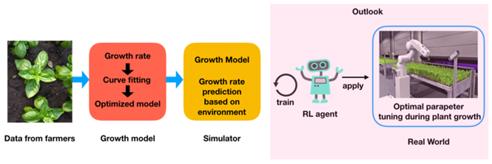
The corresponding modeling chain is illustrated in Fig. 1. It comprises four main steps, (1) image processing, (2) fitting of growth curves, (3) learning the dependence of growth parameters on environment parameters, and (4) construction of the simulator. All steps are described in detail below.
2.1 Recording and processing of plant growth data
Dataset collection
The data used in this experiment has been collected over a period of 12 months of growing multiple batches of basil. The collection of data consists of two parts:
- 1.
Environmental data (using IoT data);
- 2.
Top-down images of the crop (using cameras).
In terms of (1) environmental data, the following variables were collected from the growth chamber every 5 minutes:
- •
- •
Air temperature
- •
Relative air humidity
- •
Electrical Conductivity (EC)
- •
Oxidation Reduction Potential (ORP)
- •
Water pH
- •
Water temperature
To collect (2) top-down images of the crop, we used an 8-megapixel Raspberry Pi Camera Module 2. Crop images have been captured every 15 minutes. This low-cost camera module offers high-quality images and is suitable to deploy to both greenhouses and vertical farms to capture the growth of crops.
Processing
Upon collecting the dataset, we post-processed the images to quantify crop growth. Quantifying crop growth is done by estimating the size of the crop. This estimation is an object recognition problem consisting of two parts:
- •
Crop localization; and
- •
Crop classification.
To be able to localize the crops, a potential approach is to remove the background using simple thresholding. However, as the environment does not remain identical (e.g., crop grows, dimming of lights), simple thresholding yields unsatisfactory results when compared to statistical models. Ideally, one needs to be able to accurately localize and classify the crop regardless of size and or unfavorable illumination conditions.
In contrast to the status quo, our approach uses deep convolutional neural networks (CNN) applied to a less researched area – plant growth in controlled environment agriculture. The reasoning behind our choice is that CNNs are considered state-of-the-art in image recognition [6] thanks to their high learning capacity and robustness to the typical challenges of object recognition. To segment and classify tens of thousands of top-down images of basil, we fine-tuned a CNN using transfer learning[2]. The result is an accurate method to quantify the crop’s size.
2.2 Growth curves
To quantify the plant growth over time, we use the green canopy cover (CC) as a measure of plant size. Its development can be modeled with high average precision by the logistic growth curve [12]:
| (1) |
where is the maximum plant area, the midpoint, with , and the plant growth rate.
The data obtained from the image processing, i.e., the percentage area covered by plants, was simplified by averaging daily measurements. The reason for averaging daily measurements is to smooth out daily growth fluctuations due to light presence or absence. Individual batches were then fitted using SciPy’s curve_fit function [13]. Lower and upper bounds were set to a fixed value of 0 and 1, respectively. The values
and were obtained from fitting the model. The fitting was done continuously for all batches with a growth period of days and sub-batches starting from day 5 ().
In addition, the growth rates computed for all sub-batches can be used to iteratively estimate plant sizes at a future time step. This was only done for because the environmental parameters need to be adjusted at . However, this adjustment can be extended further into the future. It is important to note that the estimates at this time are based solely on past plant sizes and do not take into account environmental factors.

2.3 Dependence of growth parameter on environment parameters
To extend the simple growth model to a function reflecting growth dependencies on environment parameters, a model was fitted using the growth rates as target and environment parameters as input variables. Since the environment is the driving factor for plant growth, it is hypothesized that these variables can be used to predict or the change in for the next time step ().
For interpretability purposes, multiple polynomial regression models were fitted to reflect dependencies of growth rates (k) on individual environment parameters. To find optimal polynomial degrees a range of values [1, 2, 3, 4] has been tested. To improve the models relative to the model trained over the entire dataset, we binned the data into different growth stages. That is, we grouped the data into 4 bins of 25% of total area covered by plants. This suggests that optimal environmental factors change during the growth process. Figure 3 depicts such a dependency of on the pH level of water in the second quarter (25% to 50% of the final plant size). Fastest growth is obtained for pH values between 6.0 and 6.5, while smaller and especially higher values tend to slow down the growth process on average.

2.4 Model training
The training set for the simulator-model consists of Basil batches. Given our initial dataset (30 batches * 30 days), classic machine-learning methods were applied first. A complete list of tested models can be found in Table 1 below. The main input features consist of all environment variables from the current day (), and the target variable, either or , for the next day (). Other feature combinations, such as and moving averages from two to six days, were included in the test iterations.
To account for different growth stages, e.g., early growth or saturation, two different binning methods of the training data were tested in addition to training with the entire data set:
- 1.
4 sequential bins containing 25% of the data, as described in Section 2.3.
- 2.
15 bins containing 40% of the data with overlapping windows.
These bins were restricted with a lower bound of 0.05 and an upper bound of 1. This leads to smaller bins at the beginning and the end of the growth process, loosely reflecting the S-shape of the growth curve.
The dataset was then split into 80% training data and 20% test data. The validation was done using and MSE[15]. The best model for the Basil data regarding the MSE was achieved using a linear regression model with overlapping bins for predicting directly. The best model fit in terms of was achieved by a linear regression with sequential bins. The model for the simulator was chosen in terms of the smallest MSE.

| Model | Binning | MSE | |
|---|---|---|---|
| Huber Regressor | overlapping | 0.704392 | 0.008783 |
| Huber Regressor | sequential | 0.758954 | 0.007161 |
| Huber Regressor | none | 0.503647 | 0.005309 |
| Linear Regression | overlapping | 0.988588 | 0.000354 |
| Linear Regression | sequential | 0.989152 | 0.001132 |
| Linear Regression | none | 0.988169 | 0.000487 |
| Polynomial Regressor | overlapping | 0.733265 | 0.009973 |
| Polynomial Regressor | sequential | 0.792810 | 0.006454 |
| Polynomial Regressor | none | 0.629016 | 0.014098 |
| K-Nearest Neighbors | overlapping | 0.848751 | 0.004200 |
| K-Nearest Neighbors | sequential | 0.795600 | 0.005350 |
| K-Nearest Neighbors | none | 0.911697 | 0.003541 |
| Support Vector Machine | overlapping | 0.681001 | 0.006655 |
| Support Vector Machine | sequential | 0.638616 | 0.006822 |
| Support Vector Machine | none | 0.863949 | 0.003802 |
2.5 Plant growth simulator
The trained models for the various bins were implemented and tested in a simulation framework. Each growth batch was initialized with and . The duration of the simulation was set to 35 days. At each step during the simulation, random environmental variables were drawn from a normal distribution with the mean and variance of each variable in the training set.
During the simulation, the model of the bin whose center is closest to the current plant size is selected for the prediction of . The obtained prediction for was then used to calculate by subtracting the current value, i.e. the last prediction of , from this prediction:
| (2) |
Further, was normalized to accommodate for potential changes in the environment variables during the simulation. Since sudden changes in the environment may lead to unrealistically large predictions of , the following normalization has been used:
| (3) |
After adding to the next day plant size can be calculated by inserting the value into the growth curve (Eq. 1). Figure 5 depicts 10 repetitions and the final growth rate of each simulated batch.

To guide the system towards a desired target growth rate , we define the reward function as:
| (4) |
In our initial tries, we use the maximal value of observed in the data as the target value .
We compared the interaction with the simulation environment of three different strategies and observed the rewards they achieve:
- •
Random adjustments of plant environment parameters within the range of values observed in the data.
- •
Applying the same adjustments that are present in the data.
- •
Applying an AI-agent trained with PPO [11].
The results are shown in Fig. 6. While the actions performed in the recorded data are certainly favorable to achieve faster plant growth we see a clear potential for AI agents trained in this way to improve outcomes in indoor farming environments.

3 Related Work
Plant growth models aim to describe the interaction between the growth of plants and their environment [9]. Several types of plant growth models exist, with varying degrees of complexity, centered on different key physiological processes and investigated at different temporal and spatial scales [5]. An alternative is to learn the input-output relationships directly from data with the help of Machine Learning (ML), which has successfully been applied to plant growth prediction in the past. Conventional ML algorithms as well as deep learning were investigated, with LSTM [8] models giving the best results [1]. However, these models only learn to predict the regular temporal pattern of plant growth, without providing insights into the effect of environmental parameters[14]. The usefulness of reinforcement learning to steer plant behavior has been recognized before and used in the construction of several game-like simulation environments [7, 10]. Recently, RL solutions for sustainable agriculture have been proposed [3], and the first smart agriculture IoT systems based on reinforcement learning have been constructed in China [4, 16]. However, to date, no ML model exists which is able to actively control the complete growth process in an indoor farming setup, while taking into account growth speed, plant health and energy efficiency.
4 Conclusions
We developed a simulator for the automatic adjustment of environmental variables in indoor farming. We first fitted a growth curve model and subsequently trained a machine learning model to predict growth rates based on environmental variables. The resulting model could successfully be used in a simulator which enables the training of a reinforcement learning agent. Initial tests show potential for such agents to automate the control of plant environment parameters and optimize plant growth. Next, we plan to incorporate plant health objectives as well as energy efficiency objectives in the reward function and test our AI agent in a real-world setting.
Acknowledgements
We thank Innosuisse for the support within 59624.1 INNO-ICT.
References
- [1] B. Alhnaity, S. Pearson, G. Leontidis, and S. Kollias. Using deep learning to predict plant growth and yield in greenhouse environments. Acta Horticulturae, 1(1296):425–432, November 2020.
- [2] Nagender Aneja and Sandhya Aneja. Transfer Learning using CNN for Handwritten Devanagari Character Recognition. In 2019 1st International Conference on Advances in Information Technology (ICAIT), pages 293–296, July 2019. arXiv:1909.08774 [cs, eess].
- [3] Jonathan Binas, Leonie Luginbuehl, and Yoshua Bengio. Reinforcement Learning for Sustainable Agriculture. CCAI workshop at the 36th International Conference on Machine Learning, page 3, 2019.
- [4] Fanyu Bu and Xin Wang. A smart agriculture iot system based on deep reinforcement learning. Future Gener. Comput. Syst., 99:500–507, 2019.
- [5] T. Fourcaud, X. Zhang, A. Stokes, H. Lambers, and C. Korner. Plant Growth Modelling and Applications: The Increasing Importance of Plant Architecture in Growth Models. Annals of Botany, 101(8):1053–1063, August 2007.
- [6] Alexander Gomez, Augusto Salazar, and Francisco Vargas. Towards Automatic Wild Animal Monitoring: Identification of Animal Species in Camera-trap Images using Very Deep Convolutional Neural Networks. Technical Report arXiv:1603.06169, arXiv, March 2016. arXiv:1603.06169 [cs] type: article.
- [7] Yasmeen Hitti, Ionelia Buzatu, Manuel Del Verme, Mark Lefsrud, Florian Golemo, and Audrey Durand. GrowSpace: Learning How to Shape Plants. Technical Report arXiv:2110.08307, arXiv, October 2021. arXiv:2110.08307 [cs] type: article.
- [8] Sepp Hochreiter and Jürgen Schmidhuber. Long short-term memory. Neural computation, 9(8):1735–1780, 1997.
- [9] Fenni Kang. Plant growth models and methodologies adapted to their parameterization for the analysis of phenotypes. HAL open science, page 179, 2015.
- [10] Hiske Overweg, Herman N. C. Berghuijs, and Ioannis N. Athanasiadis. CropGym: a Reinforcement Learning Environment for Crop Management. Technical Report arXiv:2104.04326, arXiv, April 2021. arXiv:2104.04326 [cs] type: article.
- [11] John Schulman, Filip Wolski, Prafulla Dhariwal, Alec Radford, and Oleg Klimov. Proximal Policy Optimization Algorithms. Technical Report arXiv:1707.06347, arXiv, August 2017. arXiv:1707.06347 [cs] type: article.
- [12] Eline Vanuytrecht, Dirk Raes, Pasquale Steduto, Theodore C. Hsiao, Elias Fereres, Lee K. Heng, Marga Garcia Vila, and Patricia Mejias Moreno. AquaCrop: FAO’s crop water productivity and yield response model. Environmental Modelling & Software, 62:351–360, December 2014.
- [13] Pauli Virtanen, Ralf Gommers, Travis E. Oliphant, Matt Haberland, Tyler Reddy, David Cournapeau, Evgeni Burovski, Pearu Peterson, Warren Weckesser, Jonathan Bright, Stéfan J. van der Walt, Matthew Brett, Joshua Wilson, K. Jarrod Millman, Nikolay Mayorov, Andrew R. J. Nelson, Eric Jones, Robert Kern, Eric Larson, C J Carey, İlhan Polat, Yu Feng, Eric W. Moore, Jake VanderPlas, Denis Laxalde, Josef Perktold, Robert Cimrman, Ian Henriksen, E. A. Quintero, Charles R. Harris, Anne M. Archibald, Antônio H. Ribeiro, Fabian Pedregosa, Paul van Mulbregt, and SciPy 1.0 Contributors. SciPy 1.0: Fundamental Algorithms for Scientific Computing in Python. Nature Methods, 17:261–272, 2020.
- [14] Chunying Wang, Weiting Pan, Xubin Song, Haixia Yu, Junke Zhu, Ping Liu, and Xiang Li. Predicting Plant Growth and Development Using Time-Series Images. Agronomy, 12(9):2213, September 2022.
- [15] Wikipedia contributors. Coefficient of determination — Wikipedia, the free encyclopedia, 2022. [Online; accessed 30-November-2022].
- [16] Ni Zhou. Intelligent Control of Agricultural Irrigation Based on Reinforcement Learning. Journal of Physics: Conference Series, 1601(5):052031, August 2020.