Robust convex biclustering with a tuning-free method
Abstract
Biclustering is widely used in different kinds of fields including gene information analysis, text mining, and recommendation system by effectively discovering the local correlation between samples and features. However, many biclustering algorithms will collapse when facing heavy-tailed data. In this paper, we propose a robust version of convex biclustering algorithm with Huber loss. Yet, the newly introduced robustification parameter brings an extra burden to selecting the optimal parameters. Therefore, we propose a tuning-free method for automatically selecting the optimal robustification parameter with high efficiency. The simulation study demonstrates the more fabulous performance of our proposed method than traditional biclustering methods when encountering heavy-tailed noise. A real-life biomedical application is also presented. The R package RcvxBiclustr is available at https://github.com/YifanChen3/RcvxBiclustr.
keywords
Biclustering; Huber loss; Heavy tail; Tuning-Free; Convex optimizationbSchool of Statistics and Data Science, Jiangxi University of Finance and Economics, Nanchang, China;
cKey Laboratory of Data Science in Finance and Economics, Jiangxi University of Finance and Economics, Nanchang, China;
dDepartment of Mathematics, University College London, Gower Street, London, WC1E 6BT, United Kingdom
1 Introduction
Biclustering, which was first proposed by Hartigan et al. [1], tries to cluster rows and columns of a data matrix simultaneously. Lately, biclustering methods have been applied to a wide range of fields for data analysis and visualization such as biomedical data analysis, text mining, and recommendation system. To elaborate, in the domain of biomedical data analysis, researchers seek to identify patterns underlying the high-dimensional genetic data, which illustrate the local correlation between gene expression and patients, thus identifying subtypes of a certain disease [2, 3, 4, 5, 6, 7]. In text mining, biclustering algorithms can recognize similar document subgroups by the local correlation between documents and words [8, 9]. In recommendation system, biclustering can be used to discover the local correlation between a group of certain customers and a particular category of products, and therefore improve the efficiency of recommendations [10, 11].
In this paper, we focus on proposing a biclustering algorithm that could be used to detect the local correlation in lung cancer microarray data regardless of the heavy-tailed noise. Lung cancer has several different subtypes. Our goal is to identify whether some genes have significant correlations with certain cancer subtypes. In other words, are some genes responsible for causing or restraining certain kinds of lung cancer? This is of great importance in both theoretical medical research and application. If we succeed in finding some significant correlations between genes and cancer subtypes, doctors can use this result as a reference to further determine personalized treatment strategies according to specific subtypes.
Recently, sparse biclustering has been increasingly popular in the field of statistics. Meanwhile, this kind of algorithm has three subgroups of derivatives: sparse biclustering based on K-means, sparse biclustering based on SVD, and convex biclustering. Tan and Witten [5] extended the one-way K-means to two-way, thus proposing the SparseBC algorithm. However, since it is the derivative algorithm of one-way K-means, it shares the same limitation as one-way K-means. SparseBC takes a greedy approach, so it is sensitive to the initialization and can only reach a local optimal. Lee et al. [6] proposed a biclustering algorithm, SSVD, based on SVD innovatively. Sill et al. [12] adapted a robust tuning parameter based on SSVD and proposed the S4VD algorithm in consideration of data perturbance. Nevertheless, none of the methods above solves the two primary problems: sensitivity to initialization and local optimal. Chi et al. [7] proposed the convex biclustering algorithm (COBRA), which can be viewed as a convex optimization problem, therefore global optimal can be guaranteed and sensitivity to initialization exists no more. COBRA doesn’t need to designate the number of biclusters like SparseBC nor the number of layers like SSVD. It only has one tuning parameter, the coefficient of penalty term, . Consequently, the process of tuning the parameter is relatively trivial and efficient.
However, the effectiveness of COBRA will significantly reduce when the data contains heavy-tailed noise. Specifically, the distribution of a random variable with distribution function is said to have a heavy tail if the moment generating function of , , is infinite for all , namely, for all . Moreover, heavy-tailed noise is inevitable in high-dimensional data, so it is unrealistic to expect high-dimensional data in the fields of finance, macroeconomics, and biomedical to have sub-Gaussian distribution [13, 14, 15, 16, 17]. Huber loss [18] was proposed to mitigate the negative influence of outliers with the following form:
| (1) |
Notice that Huber loss is exactly squared error loss when . The robustness comes from the part that , where the absolute error loss serves as a buffer that controls the rising speed of squared error loss. Huber regression is also proposed to address the heavy-tailed noise problem [19]. Yohai and Maronna [20]; Mammen [21]; He and Shao [22] did thorough research on the asymptotic properties of M-estimators. On the other hand, for the non-asymptotic point of view, we refer to [23, 24, 25, 26]. Liu et al. [27] proposed robust convex clustering, which adapted the cost function and weight function of convex clustering into Huber loss, thus making it perform well when facing data containing heavy-tailed noise. Based on this thought, we extend this idea into convex biclustering by replacing the squared error term in the cost function and weight function with Huber loss.
Yet, this adaptation introduces a new parameter, the robustification parameter in Huber loss, , making not only the process of tuning the parameters time-consuming but also the parameter hard to determine. Sun et al. [26] proposed the adaptive Huber regression for robust estimation and inference whose robustification parameter is adapted to the sample size, dimension, and moments. Wang et al. [28] proposed a tuning-free method for Huber regression. Accordingly, we extend this idea into our method and put the tuning of into the iteration of the algorithm. Therefore, the proposed algorithm won’t be needing to tune the parameter manually when it comes to simulation and application, which speeds up the process and increases the accuracy.
The rest of this paper is organized as follows. In Section 2, we propose a Robust Convex BiClustering algorithm (RCBC). Section 3 proposes a tuning-free method for selecting a desirable for the algorithm, and demonstrates the cross-validation procedure we use to select the penalty parameter . Section 4 contains the result of our simulation study. In Section 5, we implement RCBC on gene data for an application. And finally, the discussion is in Section 6.
2 Robust Convex Biclustering
We seek to identify a checkboard pattern that reflects the local correlation between the features and the samples. Let be a data matrix with samples and features and be the estimated matrix generated by minimizing the following convex optimization problem
| (2) |
where , , and denotes the th column(row) of the matrix . The above equation is a fused lasso problem in which the cost function represents how well approximates and the penalty term tends to make close elements fuse with each other from both directions. The nonnegative tuning parameter controls the tradeoff between the cost function and the penalty term. When , reaches its optimal when . As increases, the close elements begin to coalesce, and the checkboard pattern starts to merge. When is sufficiently large, will tend to shrink into one bicluster with all the entries being a constant.
The cost function is a robust adaptation of squared error loss. In real life, data cannot be perfect, and heavy-tailed noise, which has a significant negative influence on squared error loss, is inevitable. Therefore, a robust version of convex biclustering will provide us with wider application fields compared to the normal version. We choose the Huber loss [18] to address the heavy-tailed noise.
The penalty term is the same as convex biclustering [7], and the weight function is also adapted with Huber loss as follows:
| (3) |
where , , and is the indicator term which is 1 if is one of ’s nearest neighbours and 0 otherwise. Note that by implementing the indicator function, we successfully make the weight function sparse. The indicator function here significantly increases the efficiency and accuracy of the algorithm by ignoring most of the useless uncorrelated rows(columns) and making the weight function sparse. Likewise, simply substitute with can we get . This weight function has a valuable property that assigns greater weights to contaminated rows(columns) that belong to the same cluster than to rows(columns) that belong to different clusters. In the later simulation and application sections, we set and , where denotes the median absolute deviation (MAD) estimator of , as default.
After analysing the formula of robust convex biclustering, we now come to the phase of solving it. Notice that if the penalty term only has regularization in one direction instead of penalizing both rows and columns, the solution will be much easier with the Alternating Direction Method of Multipliers (ADMM) [29]. However, penalizing both directions is of necessity. Dykstra-like proximal algorithm (DLPA) [30] was proposed to tackle this kind of problem by iteratively solving two convex optimization problems.
Typically, DLPA solves problems with the form
| (4) |
where and are lower semicontinuous and convex function, and is the Frobenius norm. Let , . The extension from squared error loss to Huber loss is natural as the latter is also convex. The proximal mapping in the original DLPA algorithm thus becomes
| (5) |
which happens to be the formula of robust convex clustering.
Therefore, the thought of our algorithm is straightforward. Informally, we just perform one-way robust convex clustering algorithms to rows and columns respectively in one iteration and then iterate until convergence. Yet, some details still need to be clarified. Let and be the estimated mean matrix at the th iteration of and respectively. reflects the discrepancy between and , and likewise, reflects the discrepancy between and . To make things clear, , while , . Instead of simply clustering rows and columns in each iteration, we actually cluster and . Additionally, the stop criterion is trivial. The iteration will stop until , where is the tolerance of this iteration which is efficiently small. The pseudocode of our algorithm is shown in Algorithm 1.
The one-way robust convex clustering algorithm is almost the same as Liu et al. [27] proposed except for the weight function which is adjusted to be sparse as we mentioned before. Typically, this one-way algorithm solves the constrained optimization problem
| (6) | ||||
where is an matrix, and denotes the th row of matrix . Let be an matrix and . Consequently, the corresponding augmented Lagrangian function will be
| (7) | ||||
where are primal variables, are dual variables, and is a nonnegative tuning parameter for the ADMM algorithm. The update procedure for , and is as follows:
| (8) | ||||
where is the the soft-thresholding operator, and . The detailed derivation of the one-way algorithm can be found in Appendix A.
3 Tuning Parameters
3.1 Tuning-Free Method for Selecting
The proposed RCBC has a convincing performance in dealing with heavy-tailed noise. However, the newly introduced robustification parameter brings challenges to tuning the hyperparameters with two-dimensional grid search and cross-validation, as tuning two parameters will be much more computationally demanding compared to just tuning one. In order to speed up the process of selecting the optimal parameters, we proposed a tuning-free method for selecting .
An empirical selection for in Huber’s original proposal is , which retains 95% of the asymptotic efficiency of the estimator for normally distributed data [31]. Our proposed is more correlated to the data thus being called data-driven and adaptive. In robust regression problems, a desirable should adapt to sample size , dimension , and moments for an optimal trade-off between bias and robustness [26]. Our biclustering problem can also be viewed as a high-dimensional regression problem solved by fused lasso.
| (9) |
where are vectors that come from stretching the matrices, and is an identity matrix that serves as the design matrix of the regression problem.
Therefore, the formation of our biclustering problem is almost the same as the high-dimensional adaptive Huber regression in [28] which is guided by non-asymptotic deviation analysis. Accordingly, we add a procedure for automatically updating in the original RCBC algorithm, namely updating and solving one-way clustering problems of two directions simultaneously in one iteration. Using the previous estimated , we compute as the solution to
| (10) |
where , and represents the number of rows of a matrix that not all elements are 0. See the detailed derivation and desirable statistical properties of Equation 10 in [28].
The pseudocode for this tuning-free version of RCBC is given in Algorithm 2.
3.2 Tuning with Missing Data
Our proposed RCBC algorithm has only one tuning parameter , which is also our advantage in the process of selecting the tuning parameter compared to other algorithms. As for the method of selecting the parameter of this unsupervised problem, we refer to the classic missing data method [32, 5, 7, 33], which can recast biclustering as a supervised learning problem. Here, it is detailed as Algorithm 3:
Normally, in Algorithm 3 is set to be 10 to perform 10-fold cross-validation.
4 Simulation
In this section, we compare the performance of our tuning-free biclustering algorithm (TF-RCBC), our non-tuning-free biclustering method (RCBC), COBRA [7], and spBC [5] in ten simulation settings. Our proposed methods are available as an R package at https://github.com/YifanChen3/RcvxBiclustr. COBRA and spBC can be implemented in R packages cvxbiclustr and sparseBC respectively on CRAN.
To evaluate the quality of the clustering results, we use the following metrics: the Rand index (RI), the adjusted Rand index (ARI), and the variation of information (VI). The RI [34] is the most popular measure of the similarity between two data clusterings. Nevertheless, the RI can’t ensure a result that is close to 0 when the clustering is utterly arbitrary. Accordingly, we also use the ARI [35], which corrects the flaws of RI in some way. For both RI and ARI, they take values in the range of 0 to 1, and a value that is close to 1 indicates good agreement between the two partitions. Additionally, we compared clustering results using the VI [36]. The VI is a criterion derived from information theoretic principles for comparing two clusterings of a data set. The closer its value is to the minimum value of 0, the higher similarity between the true classification situation and the clustering result.
Throughout our simulation studies, we simulate a data matrix with a checkerboard bicluster structure, where and . To assess the performance as the number of column and row clusters varied, we generated data with different numbers of biclusters. The first case is the generation of data using biclusters, where took on one of 21 equally spaced values between -5 and 5, namely . And the second case is the generation of data using biclusters, where took on one of 25 equally spaced values between -6 and 6, namely . To investigate the robustness and the effectiveness of these biclustering algorithms, we simulated the heavy-tailed random noise from the following five distribution settings and added it to each element of the data matrix:
- •
Cauchy distribution with and
- •
Log-normal distribution with and
- •
T distribution with degree of freedom
- •
Pareto distribution with scale and shape
- •
Skewed generalized t distribution [37] , where mean , variance with , shape , and skewness
As for the parameters in the weight function, we simply set for both column weight and row weight. Also, we set , where denotes the median absolute deviation (MAD) estimator of , in the non-tuning-free method’s weight function. We calculated the average mean and standard deviation of RI, ARI, and VI for 50 repeated runs of our proposed methods, COBRA, and spBC. The results for different simulation settings are summarized in Table 1.
| RI | ARI | VI | ||||||
|---|---|---|---|---|---|---|---|---|
| TF-RCBC | Cauchy | 0.9976 | (0.0026) | 0.9784 | (0.0239) | 0.0341 | (0.0330) | |
| log-normal | 0.9995 | (0.0007) | 0.9955 | (0.0059) | 0.0094 | (0.0121) | ||
| t | 0.9995 | (0.0005) | 0.9961 | (0.0046) | 0.0080 | (0.0088) | ||
| Pareto | 0.9998 | (0.0003) | 0.9979 | (0.0028) | 0.0048 | (0.0059) | ||
| sgt | 0.9997 | (0.0003) | 0.9972 | (0.0030) | 0.0059 | (0.0060) | ||
| RCBC | Cauchy | 0.9982 | (0.0025) | 0.9836 | (0.0230) | 0.0284 | (0.0357) | |
| log-normal | 0.9981 | (0.0029) | 0.9826 | (0.0266) | 0.0291 | (0.0395) | ||
| t | 0.9989 | (0.0018) | 0.9902 | (0.0163) | 0.0173 | (0.0255) | ||
| Pareto | 0.9998 | (0.0002) | 0.9980 | (0.0021) | 0.0046 | (0.0045) | ||
| sgt | 0.9994 | (0.0008) | 0.9947 | (0.0070) | 0.0108 | (0.0130) | ||
| COBRA | Cauchy | 0.9374 | (0.0002) | 0.0015 | (0.0009) | 0.7156 | (0.0084) | |
| log-normal | 0.9375 | (0.0001) | 0.0009 | (0.0006) | 0.7109 | (0.0069) | ||
| t | 0.9360 | (0.0016) | 0.0052 | (0.0025) | 0.7278 | (0.0130) | ||
| Pareto | 0.9522 | (0.0280) | 0.6074 | (0.1195) | 0.3487 | (0.0820) | ||
| sgt | 0.9593 | (0.0438) | 0.7696 | (0.1942) | 0.1792 | (0.1353) | ||
| spBC | Cauchy | 0.0624 | (0.0000) | 0.0000 | (0.0000) | 1.0000 | (0.0000) | |
| log-normal | 0.0624 | (0.0000) | 0.0000 | (0.0000) | 1.0000 | (0.0000) | ||
| t | 0.0624 | (0.0000) | 0.0000 | (0.0000) | 1.0000 | (0.0000) | ||
| Pareto | 0.7386 | (0.3202) | 0.6787 | (0.1920) | 0.4350 | (0.3195) | ||
| sgt | 0.9848 | (0.0248) | 0.9203 | (0.1147) | 0.0572 | (0.0823) | ||
| TF-RCBC | Cauchy | 0.9995 | (0.0008 | 0.9931 | (0.0105) | 0.0109 | (0.0158) | |
| log-normal | 0.9990 | (0.0016) | 0.9867 | (0.0221) | 0.0196 | (0.0284) | ||
| t | 0.9996 | (0.0009) | 0.9942 | (0.0118) | 0.0091 | (0.0161) | ||
| Pareto | 0.9997 | (0.0002) | 0.9963 | (0.0030) | 0.0068 | (0.0055) | ||
| sgt | 0.9998 | (0.0004) | 0.9973 | (0.0047) | 0.0048 | (0.0081) | ||
| RCBC | Cauchy | 0.9996 | (0.0005) | 0.9947 | (0.0064) | 0.0087 | (0.0093) | |
| log-normal | 0.9983 | (0.0022) | 0.9769 | (0.0316) | 0.0330 | (0.0412) | ||
| t | 0.9995 | (0.0014) | 0.9935 | (0.0197) | 0.0094 | (0.0257) | ||
| Pareto | 0.9997 | (0.0002) | 0.9967 | (0.0027) | 0.0058 | (0.0046) | ||
| sgt | 0.9995 | (0.0007) | 0.9934 | (0.0112) | 0.0096 | (0.0137) | ||
| COBRA | Cauchy | 0.9600 | (0.0001) | 0.0021 | (0.0012) | 0.6642 | (0.0083) | |
| log-normal | 0.9600 | (0.0001) | 0.0012 | (0.0007) | 0.6616 | (0.0067) | ||
| t | 0.9589 | (0.0015) | 0.0070 | (0.0034) | 0.6765 | (0.0189) | ||
| Pareto | 0.9815 | (0.0080) | 0.7199 | (0.0967) | 0.2422 | (0.0616) | ||
| sgt | 0.9961 | (0.0038) | 0.9560 | (0.0429) | 0.0191 | (0.0180) | ||
| spBC | Cauchy | 0.0399 | (0.0000) | 0.0000 | (0.0000) | 1.0000 | (0.0000) | |
| log-normal | 0.0399 | (0.0000) | 0.0000 | (0.0000) | 1.0000 | (0.0000) | ||
| t | 0.0399 | (0.0000) | 0.0000 | (0.0000) | 1.0000 | (0.0000) | ||
| Pareto | 0.8290 | (0.2748) | 0.7235 | (0.1481) | 0.3388 | (0.2904) | ||
| sgt | 0.9847 | (0.0162) | 0.8531 | (0.1409) | 0.0899 | (0.0787) | ||
Table 1 demonstrates the average mean and standard deviation of RI, ARI, and VI in 50 replicated runs. To make things clear, although all of our simulation settings are heavy-tailed distributions, the level of heaviness is different. Accordingly, we can separate all five heavy-tailed distribution settings into two groups: low noise group and high noise group. Low noise group contains Pareto distribution and skewed generalized t distribution, while high noise group contains Cauchy distribution, log-normal distribution, and t distribution. In low noise scenarios, even COBRA and spBC, which don’t have robust properties, can have a not bad performance. However, when the tails of the noise are becoming increasingly heavier, like in high noise group, COBRA and spBC will hardly be able to recover checkerboard patterns and consequently collapse. Despite the poor performance of COBRA and spBC, our proposed RCBC shows a consistently desirable and robust performance in both low and high noise scenarios. Also, we can see that the effectiveness of tuning-free and non-tuning-free RCBC is very close and similar to each other. Later, we will show an image example of different types of the collapse of COBRA and spBC, along with our proposed RCBC’s good performance.

(a)

(b)

(c)

(d)
Figure 1 can give us an intuitive illustration of COBRA and spBC’s bad performance when facing the data matrix contaminated by extremely heavy-tailed distributions. The estimated mean matrix of COBRA (Figure 1) is almost the same as the original data matrix (Figure 1), which represents the collapse of COBRA in high noise scenario. Moreover, the estimated mean matrix of spBC (Figure 1) is literally a constant matrix, which represents another type of collapse of spBC. These two types of collapse of the biclustering algorithms can also be reflected by Table 1 where the ARI of COBRA is close to 0 and the ARI of spBC is utterly 0 in high noise scenarios. Additionally, Figure 1 also demonstrates how our proposed RCBC perfectly recovers the underlying checkerboard patterns in this data matrix.
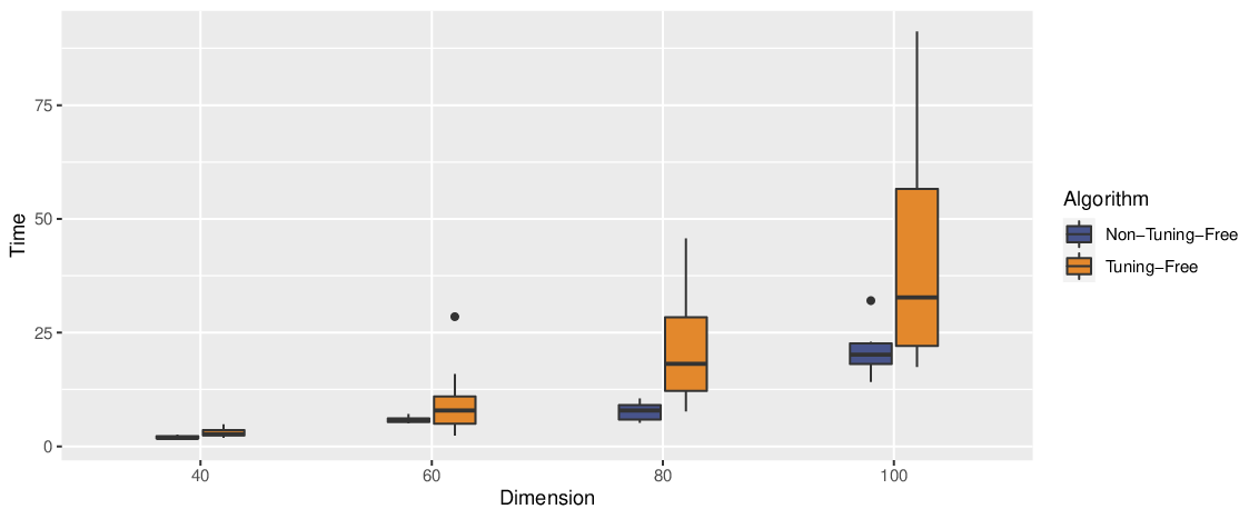
We also compare the speed of our proposed tuning-free method and non-tuning-free method. Figure 2 is a boxplot reflecting the speed of two algorithms which are rerun 10 times with noise. Although the tuning-free method is a little bit slower than the non-tuning-free one because of some extra iterative procedures in the algorithm, it does save a lot of time when selecting the optimal parameters by CV (cross-validation). The CV procedure with missing data is very computationally demanding. Therefore, reducing the number of tuning parameters from two to one is great computational simplicity and efficiency.
5 Application
We now consider applying our proposed RCBC to real-life microarray data. In this application domain, we are trying to simultaneously cluster genes and cancer subtypes. To be specific, biclustering algorithms help to identify genes that are significantly expressed for certain cancer subtypes. Lung cancer gene expression data is a very popular and classic example in biclustering problems [6, 5, 7]. The dataset contains 56 samples and 12625 genes. All 56 subjects can be divided into the following four subgroups:
- •
Normal: normal subjects(Contains 17 samples)
- •
Carcinoid: pulmonary carcinoid tumours (Contains 20 samples)
- •
Colon: colon metastases (Contains 13 samples)
- •
Small Cell: small cell carcinoma (Contains 6 samples)
We have selected the 250 genes with the greatest variance. When it comes to performing our algorithm on the data, we set for row weight and for column weight. A heatmap of the result of our proposed method is shown in Figure 3.

Figure 3 vividly illustrates our success in finding the local correlation between cancer subtypes and genes. Checkerboard patterns emerge, we can easily identify three biclusters and assign each of them to normal subjects, pulmonary carcinoid tumours, and colon metastases respectively. To elaborate, the genes in the lower part have a larger mean in pulmonary carcinoid tumours, which may be interpreted as highly expressed in this cancer subtype. Likewise, the genes in the middle and upper part have larger means in colon metastases and normal subjects respectively, which may represent the high expression in these two subtypes respectively.
Moreover, in order to verify the robust feature of RCBC in the application, we add noise to the lung cancer gene expression data. Then, we implement COBRA and RCBC both with for row weight and for column weight on this same contaminated data. Hopefully, we will still see our proposed RCBC more or less outperform COBRA. We report the result of these two algorithms in Figure 4.

(a)

(b)
From Figure 4, we can see that while COBRA almost collapse on heavy-tailed gene expression data, RCBC could still have a desirable performance on the same dataset. We can still easily identify biclusters that demonstrate the local correlation of lung cancer subtype and gene expression. Furthermore, the detailed correlation between genes and cancer subtypes is almost the same as the result on the original uncontaminated dataset. Therefore, we can say that although the data contains heavy-tailed noise, RCBC is still robust and accurate.
6 Discussion
In this paper, we proposed a robust version of convex biclustering (RCBC) to deal with the heavy tail noise in real life. The robust property is achieved by substituting the square loss with the Huber loss. Additionally, we proposed a tuning-free method for selecting the robustification parameter in order to speed up the procedure of finding the optimal parameters. We’ve shown that in extremely heavy tail scenarios, our proposed algorithm outperforms its ancestor COBRA to a large extent. Also, we manifested the feasibility of applying our algorithm to real-life biomedical data.
Despite the excellent result of our simulation study, there are some aspects to be improved. First, the speed of our algorithm is not very competitive compared to other biclustering algorithms. Accordingly, there could be some improvement in the derivation of optimization. Second, our proposed method does not allow for overlapping biclusters, i.e., each element in the data matrix can only be in one bicluster. However, although some advantages exist for overlapping biclusters in certain contexts [38], it is very complex and hard to interpret [5].
Disclosure statement
No potential conflict of interest was reported by the authors.
Funding
This work was supported by the Technology Research Project of Education Department of Jiangxi Province under Grant No. GJJ210535; National Natural Science Foundation of China under Grant No. 12161042; and China Postdoctoral Science Foundation under Grant No. 2019M662262.
References
- [1] Hartigan JA. Direct clustering of a data matrix. Journal of the american statistical association. 1972;67(337):123–129.
- [2] Lazzeroni L, Owen A. Plaid models for gene expression data. Statistica Sinica. 2002;12:61–86.
- [3] Bergmann S, Ihmels J, Barkai N. Iterative signature algorithm for the analysis of large-scale gene expression data. Physical review E. 2003;67(3):031902.
- [4] Turner HL, Bailey TC, Krzanowski WJ, et al. Biclustering models for structured microarray data. IEEE/ACM transactions on computational biology and bioinformatics. 2005;2(4):316–329.
- [5] Tan KM, Witten DM. Sparse biclustering of transposable data. Journal of Computational and Graphical Statistics. 2014;23(4):985–1008.
- [6] Lee M, Shen H, Huang JZ, et al. Biclustering via sparse singular value decomposition. Biometrics. 2010;66(4):1087–1095.
- [7] Chi EC, Allen GI, Baraniuk RG. Convex biclustering. Biometrics. 2017;73(1):10–19.
- [8] Dhillon IS. Co-clustering documents and words using bipartite spectral graph partitioning. In: Proceedings of the seventh ACM SIGKDD international conference on Knowledge discovery and data mining; 2001. p. 269–274.
- [9] Dhillon IS, Mallela S, Modha DS. Information-theoretic co-clustering. In: Proceedings of the ninth ACM SIGKDD international conference on Knowledge discovery and data mining; 2003. p. 89–98.
- [10] Hofmann T, Puzicha J. Latent class models for collaborative filtering. In: IJCAI; Vol. 99; 1999.
- [11] Alqadah F, Reddy CK, Hu J, et al. Biclustering neighborhood-based collaborative filtering method for top-n recommender systems. Knowledge and Information Systems. 2015;44(2):475–491.
- [12] Sill M, Kaiser S, Benner A, et al. Robust biclustering by sparse singular value decomposition incorporating stability selection. Bioinformatics. 2011;27(15):2089–2097.
- [13] Cont R. Volatility clustering in financial markets: empirical facts and agent-based models. In: Long memory in economics. Springer; 2007. p. 289–309.
- [14] Stock JH, Watson MW. Forecasting using principal components from a large number of predictors. Journal of the American statistical association. 2002;97(460):1167–1179.
- [15] Pan J, Shen J, Si W, et al. Resveratrol promotes mica/b expression and natural killer cell lysis of breast cancer cells by suppressing c-myc/mir-17 pathway. Oncotarget. 2017;8(39):65743.
- [16] Balcan MF, Liang Y, Gupta P. Robust hierarchical clustering. The Journal of Machine Learning Research. 2014;15(1):3831–3871.
- [17] Suzek BE, Wang Y, Huang H, et al. Uniref clusters: a comprehensive and scalable alternative for improving sequence similarity searches. Bioinformatics. 2015;31(6):926–932.
- [18] Huber PJ. Robust estimation of a location parameter. In: Breakthroughs in statistics. Springer; 1992. p. 492–518.
- [19] Huber PJ. Robust regression: Asymptotics, conjectures and monte carlo. The Annals of Statistics. 1973;1(5):799–821.
- [20] Yohai VJ, Maronna RA. Asymptotic behavior of -estimators for the linear model. The Annals of Statistics. 1979;7(2):258–268.
- [21] Mammen E. Asymptotics with increasing dimension for robust regression with applications to the bootstrap. The Annals of Statistics. 1989;17(1):382–400.
- [22] He X, Shao QM. On parameters of increasing dimensions. Journal of multivariate analysis. 2000;73(1):120–135.
- [23] Catoni O. Challenging the empirical mean and empirical variance: a deviation study. In: Annales de l’IHP Probabilités et statistiques; Vol. 48; 2012. p. 1148–1185.
- [24] Tan KM, Sun Q, Witten D. Sparse reduced rank huber regression in high dimensions. Journal of the American Statistical Association. 2022;0(0):1–11.
- [25] Ke Y, Minsker S, Ren Z, et al. User-friendly covariance estimation for heavy-tailed distributions. Statistical Science. 2019;34(3):454–471.
- [26] Sun Q, Zhou WX, Fan J. Adaptive huber regression. Journal of the American Statistical Association. 2020;115(529):254–265.
- [27] Liu C, Sun Q, Tan KM. Robust convex clustering: How does fusion penalty enhance robustness? arXiv preprint arXiv:190609581. 2019;.
- [28] Wang L, Zheng C, Zhou W, et al. A new principle for tuning-free huber regression. Statistica Sinica. 2021;31:2153–2177.
- [29] Boyd S, Parikh N, Chu E, et al. Distributed optimization and statistical learning via the alternating direction method of multipliers. Foundations and Trends® in Machine learning. 2011;3(1):1–122.
- [30] Bauschke HH, Combettes PL. A dykstra-like algorithm for two monotone operators. Pacific Journal of Optimization. 2008;4(3):383–391.
- [31] Huber PJ. Robust statistics. In: International encyclopedia of statistical science. Springer; 2011. p. 1248–1251.
- [32] Witten DM, Tibshirani R, Hastie T. A penalized matrix decomposition, with applications to sparse principal components and canonical correlation analysis. Biostatistics. 2009;10(3):515–534.
- [33] Xu QS, Li CQ, Wang X, et al. Integrative and sparse singular value decomposition method for biclustering analysis in multi-sources dataset. Chemometrics and Intelligent Laboratory Systems. 2021;211:104281.
- [34] Rand WM. Objective criteria for the evaluation of clustering methods. Journal of the American Statistical association. 1971;66(336):846–850.
- [35] Hubert L, Arabie P. Comparing partitions. Journal of classification. 1985;2(1):193–218.
- [36] Meilă M. Comparing clusterings—an information based distance. Journal of multivariate analysis. 2007;98(5):873–895.
- [37] Theodossiou P. Financial data and the skewed generalized t distribution. Management Science. 1998;44(12-part-1):1650–1661.
- [38] Madeira SC, Oliveira AL. Biclustering algorithms for biological data analysis: a survey. IEEE/ACM transactions on computational biology and bioinformatics. 2004;1(1):24–45.
Appendix A Derivation of (8)
In (7), we already have the augmented Lagrangian function. We recast the function here again:
By the ADMM algorithm, the update for and can be derived as follows:
a) Derivation for the update of :
This optimization problem can be write as:
The solution to this problem is trivial by taking the matrix derivative of :
b) Derivation for the update of :
Ignore the uncorrelated variables, and the problem is equivalent to
We can solve the above problem element-wise:
(i) When :
The Huber loss will become square error loss, so the corresponding problem will be:
Take the derivative of and set the first order derivative of the above formula to be 0 can we get
Take this result into the condition , we can have a more useful condition:
(ii) When , or equivalent to :
The corresponding optimization problem will become:
We can rewrite it into the form that can be easily solved by the soft-thresholding operator:
Thus
where is the the soft-thresholding operator.
c) Derivation for the update of :
By ignoring the uncorrelated variables and rewrite the problem row-wise, we have:
which can be viewed as a group lasso problem with the following solution:
where
d) Derivation for the update of and :