Fast Online Hashing with Multi-Label Projection
Abstract
Hashing has been widely researched to solve the large-scale approximate nearest neighbor search problem owing to its time and storage superiority. In recent years, a number of online hashing methods have emerged, which can update the hash functions to adapt to the new stream data and realize dynamic retrieval. However, existing online hashing methods are required to update the whole database with the latest hash functions when a query arrives, which leads to low retrieval efficiency with the continuous increase of the stream data. On the other hand, these methods ignore the supervision relationship among the examples, especially in the multi-label case. In this paper, we propose a novel Fast Online Hashing (FOH) method which only updates the binary codes of a small part of the database. To be specific, we first build a query pool in which the nearest neighbors of each central point are recorded. When a new query arrives, only the binary codes of the corresponding potential neighbors are updated. In addition, we create a similarity matrix which takes the multi-label supervision information into account and bring in the multi-label projection loss to further preserve the similarity among the multi-label data. The experimental results on two common benchmarks show that the proposed FOH can achieve dramatic superiority on query time up to 6.28 seconds less than state-of-the-art baselines with competitive retrieval accuracy.
Introduction
With the increasing amount of data available on the Internet, Approximate Nearest neighbor (ANN) search (Wang et al. 2017) has achieved a widespread success in many applications, e.g. computer vision and cross-modal retrieval problems. Hashing-based methods (Wang, Kumar, and Chang 2012; Liu et al. 2016; Lu, Liong, and Zhou 2017) have attracted extensive attention for ANN search due to their advantages in terms of data storage and computational efficiency. Hashing aims at mapping high-dimensional features into compact binary codes, while preserving similarities between the original space and the binary space.
Most of the existing popular hashing methods are based on batch-learning strategy (He, Wang, and Cheng 2019; Cao et al. 2021), which hinders their ability to adapt to changes as a dataset grows and diversifies, because the computational cost may become intractable and infeasible. Hence, online hashing methods have emerged, which demonstrate good performance-complexity trade-offs by updating hash functions from streaming data (Cakir et al. 2017). Online hashing focuses on updating hash functions and hash tables constantly on the basis of continual stream data with low cost (Cakir, Bargal, and Sclaroff 2017; Lu et al. 2019b; Wang, Luo, and Xu 2020).
Online hashing can be generally divided into unsupervised hashing (Leng et al. 2015; Chen et al. 2017) and supervised hashing (Lin et al. 2020; Fang, Zhang, and Liu 2021). Unsupervised online hashing is roughly based on the idea of “sketching” (Clarkson and Woodruff 2009). The sketch is a smaller feature matrix that preserves the main features of the database. By realizing matrix decomposition, the hash functions can be updated dynamically and efficiently. Supervised online hashing is mainly based on two kinds of supervision information: similarity matrix and label. The former produces a similarity matrix based on the supervision information. Then, the loss function is constructed by approximating the inner product of the paired data and corresponding similarities. The latter generates a codebook and aims at assigning each codeword a unique label, so that data with the same label will have approximate hash codes.
Although existing supervised online hashing methods update hash functions efficiently, the hash table is updated too frequent to obtain high search efficiency. Specifically speaking, since the hash functions are updated constantly, the whole hash table needs to be updated based on the latest hash functions, when a new query arrives. Otherwise, the query is embedded by the latest hash functions, but the hash codes of the database are based on previous hash functions, which is not symmetric and leads to low accuracy without doubt. However, updating the whole hash table is too time consuming with the increasing database, which is one of the core problems in online hashing.
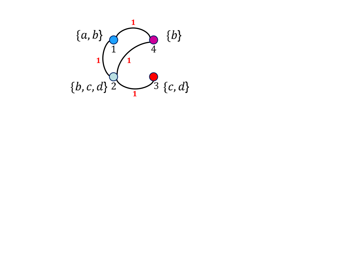
On the other hand, most of the existing supervised hashing methods contribute to construct a codebook and assign each codeword a unique label. This strategy ignores the similarity relationship among the examples, especially in the multi-label case. For example, Fig. 1 shows the label information of four points and the similarities among them. Most of the existing methods consider two examples the same (similarity equals 1) if they share at least one common label, otherwise, similarity equals 0 (no edge exists between two points in Fig. 1). Obviously, the similarity between the 3rd point and the 2nd point should be higher than that between the 4th point and the 2nd point. However, the existing methods consider these two kinds of cases the same, which is not reasonable. Besides, most of these methods just take one kind of similarity criterion into consideration, i.e., similarity matrix or label, which neglects the construction of different angels of loss functions.
In this paper, we propose a novel Fast Online Hashing (FOH) method based on multi-label projection. In order not to update the hash codes of all the database when a new query arrives, we build a query pool by randomly sampling a few central points from the database. Besides, we present a neighbor-preserving algorithm to record the nearest neighbors of the central points. The central points in the query pool and corresponding neighbors are updated based on the stream data according to the reservoir sampling strategy. In this way, when a new query arrives, a few nearest central points of the query in the query pool are returned and the corresponding potential nearest neighbors are recorded. Only the recorded data points are required to be embedded into hash codes based on the latest hash functions. Finally, Hamming distances are computed between the query hash code and the hash codes of the recorded potential nearest neighbors to obtain the retrieval results.
In addition, we make full use of the label supervision information of the data to generate the hash codes. As for the multi-label data, we present a construction algorithm to create the similarity matrix in consideration of the multi-label information of the data. Furthermore, both the similarity matrix and the label information are applied to the construction of the final loss function, which conduces to higher retrieval accuracy. To summarize, the main contributions of the proposed FOH approach are as follows.
- •
A query pool is introduced to preserve the potential nearest neighbors of the query, which makes the query time reduced. The neighbor-preserving algorithm and the reservoir sampling strategy guarantee the true neighbors of the query not to be omitted.
- •
As for multi-label supervision information, a novel similarity matrix is created to further preserve similarities among the examples. Besides, the label projection loss is brought in the final loss function.
- •
Experimental results show dramatic query time superiority in comparison to state-of-the-art supervised online hashing methods with competitive retrieval accuracy.
Related Work
One of the representative unsupervised online hashing methods is Online Sketch Hashing (SketchHash) (Leng et al. 2015). SketchHash uses a sketch matrix to preserve the main features of the data. The hash learning task is transformed into calculating several maximum eigenvalues and eigenvectors of the sketch matrix. In order to speed up the matrix decomposition, Faster Online Sketch Hashing (FROSH) (Chen et al. 2017) downexamples the random Hadamard transform to speed up the training of the sketch matrix.
Supervised online hashing learns hash functions based on the label information, which can narrow the semantic gap. Online Kernel Hashing (OKH) (Huang, Yang, and Zheng 2013) is the first attempt to update hash functions in a paired-input fashion. With an online passive-aggressive strategy, important information about the stream data is maintained. AdaptiveHash (Cakir and Sclaroff 2015a) defines a hinge-loss function and optimises the model dramatically based on SGD. Mutual Information Hashing (MIH) (Cakir et al. 2017) utilizes mutual information as the objective function and updates the hash tables based on it. Balanced Similarity for online Discrete Hashing (Lin et al. 2019b) investigates the correlation between the existing data and the new data. BSODH sets two balancing factors to solve the “imbalance problem” caused by the asymmetric graphs and optimises them by means of discretization. Hadamard Matrix Guided Online Hashing (HMOH) (Lin et al. 2020) considers the Hadamard matrix as a more discriminative codebook. By assigning each column of the Hadamard matrix a unique label as target, the hash functions are updated.

With the rapid growth of multi-modal data, multi-modal online hashing has appeared (Xie et al. 2017; Yi et al. 2021). These methods concentrate on searching for semantically related examples from one modality (e.g. image) with queries from another modality (e.g. text) in the stream data condition. The first proposed cross-modal online hashing (OCMH) (Xie, Shen, and Zhu 2016) learns shared latent matrices and variable matrices for each modality, enabling efficient update of the hash codes. Flexible Online Multi-modal Hashing (FOMH) (Lu et al. 2019a) learns the modal combination weights adaptively based on the online streaming multi-modal data. The learnt self-weighted multi-modal fusion hash codes allow flexible fusion of heterogeneous modalities even if some of them are lost. Discrete Online Cross-modal Hashing (DOCH) (Zhan et al. 2022) has been proposed recently. DOCH not only exploits the similarity between the existing data and the new data, but also considers the fine-grained semantic information to learn the binary codes of the new data. In this paper, we focus on single-modal supervised online hashing tasks.
Fast Online Hashing with Multi-label Projection
In this section, we first give the notations and the definition of the problem. Then, we describe the details of the related algorithms, including the Neighbor-Preserving Algorithm, Reservoir Sampling Strategy, Similarity Matrix Construction Algorithm, Hash Functions Updating Algorithm and Optimization Method. Finally, we state the online query process in our model. The whole framework of the proposed model is shown in Fig. 2 and elaborated in the supplementary document.
Problem Definition
Given a set of images with corresponding semantic labels , where denotes the total number of the images, denotes the dimensionality in the original space and denotes the total number of the categories. The goal of hashing is to map the image instances to hash codes , where denotes the hash code length. In order to achieve the goal, we utilize the most common linear projection based hash functions which are defined as
| (1) |
where denotes the projection matrix and contributes to the -th hash bit. The sign function is defined as
| (2) |
The similarity preserving objective will be defined later.
As for the online learning problem, the data comes in a streaming fashion. Therefore, the examples are not all used at once (Lin et al. 2019a). For subsequent convenience, we distinguish the related representations between the new stream data and the accumulated existing data. Specifically, let denote the new input stream data at stage , where denotes the batch size (size of the stream data). The corresponding labels are denoted as . The existing data is denoted as , where denotes the total number of the existing data and . The corresponding label matrix is denoted as . Correspondingly, we denote , as the learnt binary codes at stage of the stream data and the existing data, respectively.
Neighbor-Preserving Algorithm
The aim of the neighbor-preserving algorithm is to keep the nearest neighbors of each central point up to date in consideration of the latest hash functions at stage . First, the hash codes of the new stream data () are computed as
| (3) |
Let denote the set of the central points, where denotes the total number of the central points. Let denote the nearest neighbors of the -th central point, where denotes the number of the nearest neighbors of each central point. Hence, denotes the set of all the potential neighbors. Notice that is not disjoint. Then, the hash codes of the central points () and the potential points () are calculated as
| (4) |
| (5) |
For subsequent convenience, we construct a function which is defined as following:
| (6) |
Suppose and denote two hash matrices, where and denote the numbers of hash codes in and , respectively. denotes the Hamming distance matrix. Specifically, the -th column in denotes Hamming distances between -th column in and all the columns in . returns the indices of the first neighbors with smallest values in . Finally, the nearest neighbors of the -th central point () are updated as following:
| (7) |
In this way, the potential neighbors can be updated dynamically with the increasing stream data.
Reservoir Sampling Strategy
After the stream data are accumulated for several rounds, we need to update a part of the central points in the query pool and the corresponding nearest neighbors based on the reservoir sampling strategy. The nearest neighbors of the -th updated central point () are calculated as
| (8) |
where denotes the hash code of the -th updated central point and denotes the number of the updated central points.
Similarity Matrix Construction Algorithm
As for multi-label supervision information, traditional supervised methods set the similarity between two examples as one if they share at least one common label, otherwise as zero. Obviously, this kind of binarization on the similarities ignores the detailed label sharing information among the instances. Here, we propose a similarity matrix construction algorithm to solve the above problem. Suppose denotes two examples and denotes the corresponding labels. We define and denote the numbers of the labels that the two instances contain, respectively. Then, we have
| (9) |
| (10) |
where denotes the number of the common labels that and share. Hence, the similarity between and is computed as
| (11) |
We further clarify the meanings of these notations. denotes the similarity between and from -th example’s point of view and denotes the similarity between and from -th example’s point of view. Finally, we just take the average of them to define the similarity between the two examples, which means that every instance is treated equally in our algorithm. We also provide an example based on the proposed similarity matrix construction algorithm in the supplementary document.
Hash Functions Updating Algorithm
In this part, we construct an integrated loss function to update the hash functions dynamically. In order to preserve similarity between the original space and Hamming space, we take both the similarity matrix and label information into consideration.
In view of the similarity matrix, the hash functions should be updated by minimizing the error between the similarity matrix and inner product of the hash codes. We utilize Frobenius-norm to express the formulation as
| (12) |
where is created based on the new stream data and the existing data with the proposed similarity matrix construction algorithm. It is worth noticing that in the single-label case, the similarity is defined as
| (13) |
Notice that the size of the stream data and existing data may not be the same, which contributes to an asymmetric similarity graph. Furthermore, most of the data pairs are probably dissimilar, which results in a sparse similarity matrix. To solve the above imbalance problem, we add two balance factors and as weights for similar and dissimilar examples, respectively. We set (, ), the Hamming distances among similar pairs are minified, whereas that among dissimilar pairs are enlarged (Lin et al. 2019b). In addition, we add the quantization error on the new stream data:
| (14) |
As for the label information, we construct a label projection loss to make full use of the labels. Specifically, the labels of both the stream data and existing data are projected to approach their corresponding hash codes, which is formulated as
| (15) |
where denotes the projection matrix to map the labels into hash codes. The label projection loss can make the binary codes more distinguishable and alleviate the imbalance problem caused by the coarse-grained similarity matrices effectively.
Optimization Method
Due to the binary constraints, the optimization problem of Eq. 16 is non-convex with respect to . In order to find a feasible solution, we adopt an alternating optimization approach by updating one variable with the rest fixed until convergence.
① By fixing other variables except for , we update with a close-formed solution as
| (17) |
where is an identity matrix.
② By fixing other variables except for , we get a closed-form solution of :
| (18) |
where is an identity matrix.
③ By fixing other variables except for , we rewrite Eq.16 to obtain the solution of via the following optimization problem
| (19) |
where the const items imply that they are not related to solving . Inspired by the recent advance on binary codes optimization (Xu, Lai, and dong Chen 2020), we obtain
| (20) |
where . Then, we have the closed form solution of as:
| (21) |
④ By fixing other variables except for , the sub-optimization of Eq.16 is equivalent to
| (22) |
The above formulation is equivalent to
| (23) |
Similarly, we ignore irrelevant items to . For convenience, the optimization problem in Eq. 23 is rewritten as
| (24) |
where . Since it is difficult to optimize directly, we optimize each hash bit one by one. Thus, we obtain a closed form solution for each hash bit by extending Eq. 24 to the following form:
| (25) |
where and denote the hash bits to be updated and fixed, respectively. This is also suitable for the meanings of and . Therefore, we obtain a solution for solving as
| (26) |
| Methods | CIFAR-10 | FLICKR-25K | ||||||
|---|---|---|---|---|---|---|---|---|
| Updating time (s) | Query time (s) | Updating time (s) | Query time (s) | |||||
| 32-bits | 48-bits | 32-bits | 48-bits | 32-bits | 48-bits | 32-bits | 48-bit | |
| OKH | 0.03 | 0.03 | 8.46 | 5.48 | 0.13 | 0.10 | 8.70 | 3.84 |
| AdaptHash | 0.15 | 0.21 | 8.47 | 5.29 | 0.19 | 0.11 | 11.3 | 4.58 |
| OSH | 0.27 | 0.21 | 8.79 | 5.27 | 0.18 | 0.13 | 6.90 | 3.10 |
| MIHash | 0.27 | 0.25 | 8.46 | 5.29 | 0.19 | 0.13 | 6.87 | 3.05 |
| BSODH | 0.26 | 0.24 | 8.91 | 5.90 | 0.15 | 0.10 | 7.36 | 4.40 |
| HMOH | 0.17 | 0.27 | 9.25 | 5.84 | 0.15 | 0.09 | 7.01 | 4.50 |
| FOH | 0.02 | 0.02 | 2.18 | 1.33 | 0.01 | 0.01 | 2.45 | 2.85 |
To implement the whole algorithm, we first initialize and with a standard Gaussian distribution. Then the above four steps are repeated until convergence.
Online Query Process
When a new query arrives, suppose the latest hash function is . First, the hash code of the query () is computed as
| (27) |
Given the hash codes of the central points , we search for the nearest central points of the query point in the query pool and return the corresponding potential neighbors of () by
| (28) |
where denotes the number of the returned central points. Then, the hash codes of the potential neighbors () are calculated as
| (29) |
Finally, the retrieval results () are computed as
| (30) |
where denotes the number of the required returned nearest neighbors of the query point.
Throughout the whole online query process, we find that the query time is dramatically reduced. One reason is that the number of data whose binary codes need to be updated is declined. The other reason is that the online Hamming distances calculation time and the hash codes sorting time are both decreased.
Experiments
In this section, we conduct experiments on two common datasets: CIFAR-10 (Krizhevsky 2009) and FLICKR-25K (Huiskes and Lew 2008) to verify the efficiency and effectiveness of the proposed Fast Online Hashing (FOH).
Datasets and Evaluation Protocols
CIFAR-10 is a widely used image retrieval dataset containing 60,000 images in 10 different categories. We randomly select 1,000 examples as the query set and the rest is regarded as the base set. Furthermore, 20,000 images are randomly sampled from the base set as the training set. In order to simulate the stream data, we divide the training set into 10 blocks with 2,000 examples in each block.
FLICKR-25K contains 25,000 images annotated by 24 provided labels. We select the images that own at least 20 tags. Hence, 20,015 examples are obtained for our experiment. We randomly select 2,000 examples as the test and the rest are served as both the training set and base set. For online hashing, we divide the training set into nine blocks, with the first eight blocks each containing 2,000 examples and the ninth block containing 2,015 examples.
We evaluate the accuracy performance of the online hashing methods using three criteria: Recall@, Precision@ and mAP. Recall@ is calculated by the percentage of the true neighbors in the whole true neighbor set, whereas Precision@ is calculated using the percentage of the true neighbors in the result set. The mAP is calculated based on the mean value of the Precision@ for all true neighbors.
Baselines and Settings
In order to reveal the superiority of FOH, we compare with several state-of-the-art online hashing baselines, including Online Kernel Hashing (OKH) (Huang, Yang, and Zheng 2013), Adaptive hashing (AdaptHash) (Cakir and Sclaroff 2015a), Online Supervised Hashing (OSH) (Cakir and Sclaroff 2015b), OH with Mutual Information (MIHash) (Cakir et al. 2017), Towards Optimal Discrete Online Hashing with Balanced Similarity (BSODH) (Lin et al. 2019b) and Hadamard Matrix Guided Online Hashing (HMOH) (Lin et al. 2020). We use a pre-trained VGG16 (Simonyan and Zisserman 2015) for all the baselines to extract the original real-value image features.
Here, we provide the exact values of the parameter configurations in Tab. 2. Review that denotes the number of the central points in the query pool, denotes the number of the nearest neighbors of each central point, denotes the number of the returned central points when a new query arrives, denotes the hyper-parameters in the objective function.
| Dataset | u | v | ||||||
|---|---|---|---|---|---|---|---|---|
| CIRAR-10 | 500 | 500 | 10 | 0.8 | 1.2 | 0.5 | 0.6 | 0.6 |
| FLICKR-25K | 200 | 500 | 10 | 0.8 | 1.5 | 0.5 | 0.5 | 5 |
| Methods | CIFAR-10 | FLICKR-25K | ||||||||
|---|---|---|---|---|---|---|---|---|---|---|
| 16-bits | 32-bits | 48-bits | 64-bits | 128-bits | 16-bits | 32-bits | 48-bits | 64-bits | 128-bits | |
| OKH | 0.134 | 0.223 | 0.252 | 0.268 | 0.350 | 0.531 | 0.536 | 0.532 | 0.535 | 0.537 |
| AdaptHash | 0.138 | 0.216 | 0.297 | 0.305 | 0.293 | 0.544 | 0.545 | 0.547 | 0.548 | 0.555 |
| OSH | 0.126 | 0.129 | 0.131 | 0.127 | 0.125 | 0.540 | 0.542 | 0.547 | 0.550 | 0.561 |
| MIHash | 0.640 | 0.675 | 0.668 | 0.667 | 0.664 | 0.535 | 0.539 | 0.541 | 0.545 | 0.546 |
| BSODH | 0.604 | 0.689 | 0.656 | 0.709 | 0.711 | 0.535 | 0.540 | 0.542 | 0.547 | 0.55 |
| HMOH | 0.732 | 0.723 | 0.734 | 0.737 | 0.749 | 0.548 | 0.551 | 0.558 | 0.561 | 0.565 |
| FOH | 0.685 | 0.734 | 0.746 | 0.758 | 0.763 | 0.585 | 0.604 | 0.605 | 0.610 | 0.615 |
Results and Analysis
To verify the efficiency of FOH, we conduct experiments on the hash table updating time and online query time on two datasets. As shown in Tab. 1, the baselines performs similarly. However, FOH obtains dramatic reduction on both the updating time and query time. Specifically, FOH yields up to 6.28 seconds and 4.42 seconds less query time on CIFAR-10 and FLICKR-25K, respectively. We also compare the training time of FOH with other baselines in Tab. 4. We find that the training time of FOH is relatively low.
In addition, we also make a comparison on the retrieval accuracy of FOH and state-of-the-art baselines. Tab. 3 shows the mAP scores with hash bits from 16 to 128 bits on two datasets. Fig. 3 shows the precision-recall curves of different online hashing methods with 32, 48 and 64 hash bits on CIFAR-10. It is obvious that FOH gets the highest accuracy with most of the hash bits, which reveals that FOH is competitive in consideration of accuracy. More experimental results and analysis are displayed in the supplementary document.
| Methods | Training time (s) | |||
| CIFAR-10 | FLICKR-25K | |||
| 32-bits | 48-bits | 32-bits | 48-bits | |
| OKH | 4.78 | 5.62 | 4.70 | 5.30 |
| AdaptHash | 20.8 | 42.3 | 12.3 | 19.5 |
| OSH | 93.5 | 128 | 60.1 | 90.2 |
| MIHash | 120 | 152 | 80.2 | 102 |
| BSODH | 20.6 | 21.6 | 3.09 | 3.22 |
| HMOH | 7.04 | 10.5 | 2.85 | 3.09 |
| FOH | 19.5 | 21.7 | 3.40 | 4.27 |
Ablation Study
We configure three variants of FOH to investigate the impacts on accuracy: FOH-Q that removes the query pool, FOH-L that constructs the loss function without label projection, FOH-S that utilizes the traditional similarity matrix in the multi-label case.
| Variants | CIFAR-10 | FLICKR-25K | ||
|---|---|---|---|---|
| 32-bits | 48-bits | 32-bits | 48-bits | |
| FOH-Q | 0.747 | 0.759 | 0.595 | 0.599 |
| FOH-L | 0.717 | 0.737 | 0.583 | 0.592 |
| FOH-S | - | - | 0.554 | 0.555 |
| FOH | 0.734 | 0.746 | 0.598 | 0.605 |
As reported in Tab. 5, we can observe that FOH-L and FOH-S both contribute sufficiently to performance improvement. In comparison with FOH-Q, we find that there is little difference on accuracy by building the query pool. However, it can speed up the query process dramatically. In comparison with FOH-L, we confirm that the label projection loss is crucial for learning. FOH-S shows the biggest performance gap with FOH (4.4% and 5% improvement on 32 and 48 hash bits, respectively), which demonstrates that it is indeed effective to gain accuracy by utilizing the proposed similarity matrix construction algorithm.
Tab. 6 shows how the central points updating frequency affects the retrieval accuracy on two datasets with 32 hash bits (2-b denotes updating the central points when 2 batches of stream data come). Ther are 10 batches in total in CIFAR-10 and 9 batches in total in FLICKR-25K. We find that the mAP drop is very small with the decrease of the updating frequency of the central points. Our implementation of this paper is publicly available on GitHub at: https://github.com/caoyuan57/FOH.
| Datasets | 1-b | 2-b | 3-b | 4-b | 5-b |
|---|---|---|---|---|---|
| CIFAR-10 | 0.73403 | 0.72992 | 0.72828 | 0.72626 | 0.72529 |
| FLICKR-25K | 0.60448 | 0.60134 | 0.59955 | 0.59791 | 0.59135 |
Conclusion
In this paper, we propose a novel fast online hashing model that can speed up the online query time dramatically. To achieve this goal, we build a query pool to retain the potential neighbors with the proposed neighbor-preserving algorithm and reservoir sampling strategy. Furthermore, in order to make full use of the supervision information in the multi-label case, we present a similarity construction algorithm. In the end, an integrated loss function is constructed in consideration of both the similarity matrix and label projection, which contributes to more discriminative hash codes. The experimental results show significant reduction in online query time with competitive retrieval accuracy on two common datasets.
Acknowledgment
This work is supported by the NSFC Grant Nos. 62202438, 62172090; the Natural Science Foundation of Shandong Province Grant No. ZR2020QF041; the 69th batch of China Postdoctoral Science Foundation Grant No. 862105020017; the 22th batch of ISN Open Fund Grant No. ISN22-21; the CAAI-Huawei MindSpore Open Fund; the Alibaba Group through Alibaba Innovative Research Program; the Fundamental Research Funds for the Central Universities Grant No. 842113037. We thank the Big Data Computing Center of Southeast University for providing the facility support on the numerical calculations in this paper.
References
- Cakir, Bargal, and Sclaroff (2017) Cakir, F.; Bargal, S. A.; and Sclaroff, S. 2017. Online supervised hashing. Computer Vision and Image Understanding, 156: 162–173.
- Cakir et al. (2017) Cakir, F.; He, K.; Adel Bargal, S.; and Sclaroff, S. 2017. Mihash: Online hashing with mutual information. In Proceedings of the IEEE International Conference on Computer Vision, 437–445.
- Cakir and Sclaroff (2015a) Cakir, F.; and Sclaroff, S. 2015a. Adaptive hashing for fast similarity search. In Proceedings of the IEEE International Conference on Computer Vision, 1044–1052.
- Cakir and Sclaroff (2015b) Cakir, F.; and Sclaroff, S. 2015b. Online supervised hashing. In IEEE International Conference on Image Processing, 2606–2610.
- Cao et al. (2021) Cao, Y.; Liu, J.; Qi, H.; Gui, J.; Li, K.; Ye, J.; and Liu, C. 2021. Scalable Distributed Hashing for Approximate Nearest Neighbor Search. IEEE Transactions on Image Processing, 31: 472–484.
- Chen et al. (2017) Chen, X.; King, I.; Lyu, M. R.; et al. 2017. FROSH: FasteR online sketching hashing. In Uncertainty in Artificial Intelligence,, 1–10.
- Clarkson and Woodruff (2009) Clarkson, K. L.; and Woodruff, D. P. 2009. Numerical linear algebra in the streaming model. In Proceedings of the annual ACM Symposium on Theory of Computing, 205–214.
- Fang, Zhang, and Liu (2021) Fang, Y.; Zhang, H.; and Liu, L. 2021. Label projection online hashing for balanced similarity. Journal of Visual Communication and Image Representation, 80: 103314.
- He, Wang, and Cheng (2019) He, X.; Wang, P.; and Cheng, J. 2019. K-nearest neighbors hashing. In Proceedings of the IEEE Conference on Computer Vision and Pattern Recognition, 2839–2848.
- Huang, Yang, and Zheng (2013) Huang, L.-K.; Yang, Q.; and Zheng, W.-S. 2013. Online hashing. In Proceedings of the International Joint Conference on Artificial Intelligence, 1422–1428.
- Huiskes and Lew (2008) Huiskes, M. J.; and Lew, M. S. 2008. The mir flickr retrieval evaluation. In Proceedings of the ACM International Conference on Multimedia Information Retrieval, 39–43.
- Krizhevsky (2009) Krizhevsky, A. 2009. Learning multiple layers of features from tiny images.
- Leng et al. (2015) Leng, C.; Wu, J.; Cheng, J.; Bai, X.; and Lu, H. 2015. Online sketching hashing. In Proceedings of the IEEE Conference on Computer Vision and Pattern Recognition, 2503–2511.
- Lin et al. (2019a) Lin, M.; Ji, R.; Chen, S.; Zheng, F.; Sun, X.; Zhang, B.; Cao, L.; Guo, G.; and Huang, F. 2019a. Supervised online hashing via similarity distribution learning. arXiv preprint arXiv:1905.13382.
- Lin et al. (2020) Lin, M.; Ji, R.; Liu, H.; Sun, X.; Chen, S.; and Tian, Q. 2020. Hadamard matrix guided online hashing. International Journal of Computer Vision, 128(8): 2279–2306.
- Lin et al. (2019b) Lin, M.; Ji, R.; Liu, H.; Sun, X.; Wu, Y.; and Wu, Y. 2019b. Towards optimal discrete online hashing with balanced similarity. In Proceedings of the AAAI Conference on Artificial Intelligence, volume 33, 8722–8729.
- Liu et al. (2016) Liu, L.; Lin, Z.; Shao, L.; Shen, F.; Ding, G.; and Han, J. 2016. Sequential discrete hashing for scalable cross-modality similarity retrieval. IEEE Transactions on Image Processing, 26(1): 107–118.
- Lu, Liong, and Zhou (2017) Lu, J.; Liong, V. E.; and Zhou, J. 2017. Deep hashing for scalable image search. IEEE Transactions on Image Processing, 26(5): 2352–2367.
- Lu et al. (2019a) Lu, X.; Zhu, L.; Cheng, Z.; Li, J.; Nie, X.; and Zhang, H. 2019a. Flexible online multi-modal hashing for large-scale multimedia retrieval. In Proceedings of the ACM International Conference on Multimedia, 1129–1137.
- Lu et al. (2019b) Lu, X.; Zhu, L.; Cheng, Z.; Song, X.; and Zhang, H. 2019b. Efficient discrete latent semantic hashing for scalable cross-modal retrieval. Signal Processing, 154: 217–231.
- Simonyan and Zisserman (2015) Simonyan, K.; and Zisserman, A. 2015. Very deep convolutional networks for large-scale image recognition. In International Conference on Learning Representations, 1–14.
- Wang, Kumar, and Chang (2012) Wang, J.; Kumar, S.; and Chang, S.-F. 2012. Semi-supervised hashing for large-scale search. IEEE Transactions on Pattern Analysis and Machine Intelligence, 34(12): 2393–2406.
- Wang et al. (2017) Wang, J.; Zhang, T.; Sebe, N.; Shen, H. T.; et al. 2017. A survey on learning to hash. IEEE Transactions on Pattern Analysis and Machine Intelligence, 40(4): 769–790.
- Wang, Luo, and Xu (2020) Wang, Y.; Luo, X.; and Xu, X.-S. 2020. Label embedding online hashing for cross-modal retrieval. In Proceedings of the 28th ACM International Conference on Multimedia, 871–879.
- Xie et al. (2017) Xie, L.; Shen, J.; Han, J.; Zhu, L.; and Shao, L. 2017. Dynamic multi-view hashing for online image retrieval. In Proceedings of the International Joint Conference on Artificial Intelligence.
- Xie, Shen, and Zhu (2016) Xie, L.; Shen, J.; and Zhu, L. 2016. Online cross-modal hashing for web image retrieval. In Proceedings of the AAAI Conference on Artificial Intelligence, volume 30.
- Xu, Lai, and dong Chen (2020) Xu, X.; Lai, Z.-H.; and dong Chen, Y. 2020. Relaxed locality preserving supervised discrete hashing. IEEE Transactions on Big Data.
- Yi et al. (2021) Yi, J.; Liu, X.; Cheung, Y.-m.; Xu, X.; Fan, W.; and He, Y. 2021. Efficient online label consistent hashing for large-scale cross-modal retrieval. In IEEE International Conference on Multimedia and Expo, 1–6. IEEE.
- Zhan et al. (2022) Zhan, Y.-W.; Wang, Y.; Sun, Y.; Wu, X.-M.; Luo, X.; and Xu, X.-S. 2022. Discrete online cross-modal hashing. Pattern Recognition, 122: 108262.