Straggler-Resilient Differentially-Private
Decentralized Learning

We use uppercase and lowercase letters for random variables (RVs) and their realization (both scalars and vectors), respectively, and italics for sets, e.g., $X$, $x$, and $\mathcal{X}$ represent a RV, a scalar/vector, and a set, respectively. An exception to this rule is $\tau$ which denotes the model description, also referred to as the token. Matrices are denoted by uppercase letters, their distinction from RVs will be clear from the context. Vectors are represented as row vectors and the transpose of a vector or a matrix is denoted by $(\cdot)^{\top}$. The expectation of a RV $X$ is denoted by $\mathbb{E}\left[X\right]$. We define $[n]\triangleq\{1,2,\dotsc,n\}$, while $\mathbb{N}$ denotes the set of natural numbers and $\mathbb{R}$ the set of real numbers. The (sub)gradient of a function $f(x)$ is denoted by $\nabla f(x)$, while the $\ell_{p}$-norm of a length-$n$ vector $x=(x_{1},\ldots,x_{n})\in\mathbb{R}^{n}$ is denoted by $\lVert x\rVert_{p}=\left(\sum_{i=1}^{n}|x_{i}|^{p}\right)^{\nicefrac{{1}}{{p}}}$, where $|\cdot|$ denotes absolute value. The base of the natural logarithm is denoted by ${\mathrm{e}}$, while $\log$ denotes natural logarithm. $\mathcal{N}\left({\mu},{\sigma^{2}I_{d}}\right)$ denotes the $d$-dimensional Gaussian (uncorrelated) distribution with mean $\mu$ and standard deviation $\sigma$ of each component, where $I_{d}$ is the identity matrix of size $d$. $X\sim\mathcal{P}$ denotes that $X$ is distributed according to the distribution $\mathcal{P}$, while $x\sim\mathcal{P}$ denotes a sample $x$ taken from $\mathcal{P}$. We denote by $\mathcal{D}\sim_{u}\mathcal{D}^{\prime}$ the fact that datasets $\mathcal{D}=\cup_{v\in\mathcal{V}}\mathcal{D}_{v}$ and $\mathcal{D}^{\prime}=\cup_{v\in\mathcal{V}}\mathcal{D}_{v}^{\prime}$ are the same except perhaps for the dataset of user $u$, i.e., $\mathcal{D}_{v}=\mathcal{D}_{v}^{\prime}$ for all $v\neq u$, where $\mathcal{V}$ is some set of users. Standard order notation $O(\cdot)$ is used for asymptotic results.

Consider a decentralized network of $n$ honest-but-curious nodes (users) $\mathcal{V}=\{v_{1},\dotsc,v_{n}\}$ with a decentralized dataset $\mathcal{D}=\cup_{v\in\mathcal{V}}\mathcal{D}_{v}$ where $\mathcal{D}_{v}=\bigl\{(x^{(v)}_{i},y^{(v)}_{i})\bigr\}_{i=1}^{\kappa}$, $(x^{(v)}_{i},y_{i}^{(v)})\in\mathcal{R}\subseteq\mathbb{R}^{d_{\mathrm{x}}}\times\mathbb{R}^{d_{\mathrm{y}}}$, for some set $\mathcal{R}$ and $d_{\mathrm{x}},d_{\mathrm{y}},{\kappa}\in\mathbb{N}$, is the private dataset of node $v\in\mathcal{V}$.

The nodes want to compute some function together based on their datasets but want to keep their datasets private. For that, they employ a decentralized protocol where a token $\tau\in\mathcal{W}$, for some convex set $\mathcal{W}\subseteq\mathbb{R}^{d}$, travels between the nodes according to some predefined (but potentially randomized) path. When receiving the token the $r$-th time and the global time is $h$, the node $v$ updates it as $\tau\leftarrow g^{(v)}_{r}(\tau;\,\mathtt{state}_{v}(h))$, and sends it further. Here, $\mathtt{state}_{v}(h)$ encapsulates all the information available to the node $v$ at time $h$, e.g., the available data points and the results of previous calculations. It can also include some source of randomness. We assume that the computation in each node $v$ during the $r$-th visit of the token takes random time $T^{(v)}_{r}$. Hence, the computation of $g^{(v)}_{r}(\cdot,\cdot)$ takes time at most $T^{(v)}_{r}$ as the token may be updated before the entire computation is finished.²² 2 The RVs $T^{(v)}_{r}$ are assumed to be independent and identically distributed (i.i.d.) which is in accordance with the literature, where typically stragglers are generated uniformly at random, except for a few works, e.g., [44, 56] that consider a model where nodes tend to remain stragglers for a long time, violating the i.i.d. assumption on the RVs $T^{(v)}_{r}$. We consider a model where $T^{(v)}_{r}$ is comprised of a deterministic constant part (the time it takes for an actual computation) and a random part. Also, we assume that communication between any two nodes is noiseless and takes constant time $\chi$, and hence the constant part of the computation time can be set to zero. At the end of the protocol, the token $\tau$ is distributed among the nodes, which allows for calculating the desired result. This final distribution takes constant overhead time and is therefore ignored.

For a decentralized protocol $\mathcal{A}$, we denote by $\mathcal{A}(\mathcal{D})$ the (random) transcript of all messages sent or received by all the users, i.e., $\mathcal{A}(\mathcal{D})$ are all the triples $(u,w,v)$, if $u\in\mathcal{V}$ sent a message with content $w$ to $v\in\mathcal{V}$. However, due to the decentralized nature of $\mathcal{A}$, the user $v$ only has access to the subset of $\mathcal{A}(\mathcal{D})$ consisting of the messages she sent or received, and we denote this view by $\mathcal{O}_{v}(\mathcal{A}(\mathcal{D}))=\{(u,w,u^{\prime})\in\mathcal{A}(\mathcal{D}):\text{$u=v$ or $u^{\prime}=v$}\}$. Let $\Omega$ denote the set of all possible views, i.e., $\mathcal{O}_{v}(\mathcal{A}(\mathcal{D}))\in\Omega$ for all possible parameters and realizations.

We accept the notion of NDP introduced in [11].

NDP measures how much the information collected by node $v$ depends on the dataset of node $u$. In the special case that all nodes can observe all messages, i.e., $\mathcal{O}_{v}$ is the identity map, NDP boils down to conventional LDP [57]. When processing information in a decentralized manner with no central coordinating entity, and when there is no third party (on top of the topology) observing all messages sent, NDP is a more natural privacy measure than DP or LDP.

We suggest the following protocol inspired by projected noisy stochastic gradient descent to solve (1). The token $\tau$ keeps the current estimate of the optimal point $\tau^{*}$ and follows a possibly randomized path over the available nodes $\mathcal{V}$. To speed up the process, the token waits up to a threshold time $t_{\mathrm{skip}}$ and, if the computation has not finished by that time, the token is forwarded further without an update.³³ 3 In practice, acknowledgments can identify straggling nodes: if the token is sent to the next node in line and not acknowledged within a threshold time, it is forwarded to the next node in line, etc. In our notation, it means that the calculation in each node $v$ is

where $\eta_{h}$ is the step size (learning rate), $\Pi_{\mathcal{W}}$ denotes the Euclidean projection onto the set $\mathcal{W}$, and $N_{h}$ is noise with zero mean and standard deviation $\sigma_{h}$. The noise $N_{h}$ is added in order to protect the privacy of the local datasets, and the standard deviation $\sigma_{h}$ is chosen so a certain level of NDP is ensured.⁴⁴ 4 The noise follows $\mathcal{N}\left({0},{\sigma_{h}^{2}}\right)$, where $\sigma_{h}=\frac{k\sqrt{8\log(\nicefrac{{1.25}}{{\delta}})}}{\varepsilon}$, $\varepsilon>0$, and $0<\delta<1$. In this work, we consider the gamma distribution (including the exponential distribution) and the Pareto type II (also known as Lomax) distribution for $T_{r}^{(v)}$, which are well-established models in the literature, see, e.g., [58, 56, 59]. Since we assume that the RVs $T_{r}^{(v)}$ are i.i.d., we simplify the notation in the following by letting $T\equiv T_{r}^{(v)}$.

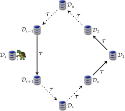
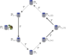
The algorithm stops when a predefined convergence requirement is fulfilled. We refer to the algorithm detailed above as the skipping scheme with parameter $t_{\mathrm{skip}}$, which can be optimized in order to reduce either the convergence time and/or the privacy leakage. In the special case of $t_{\mathrm{skip}}=\infty$, it reduces to a scheme for which the token always waits. We denote by $p=\Pr[T>t_{\mathrm{skip}}]$ the probability of skipping a node. The formal algorithm is given in Algorithm 1, where the output $\ell$ denotes its execution latency and $\tau_{h_{\max}}$ the final value of the token after $h_{\max}$ steps.

We use Algorithm 1 in two special cases as outlined below and illustrated in Fig. 1. For both schemes, the noise variance is fixed throughout the algorithm, i.e., $\sigma_{h}=\sigma$, $\forall\,h$, and we assume, for simplicity, that $h_{\max}$ is a multiple of $n$ in the rest of the paper.

• •

  First, we consider an update schedule in which the nodes in $\mathcal{V}$ are processed along a logical ring, i.e., the node path sequence of Algorithm 1 is $(v^{(1)},\ldots,v^{(h_{\max})})=((v_{1},\ldots,v_{n}),(v_{1},\ldots,v_{n}),\ldots,(v_{1},\ldots,v_{n}))$. The corresponding scheme is denoted by Skip-Ring.

• •

  Second, we consider a randomized version of the logical ring, denoted by Skip-Rand-Ring. Each round over the ring can be seen as a random walk on the set of nodes, but without replacement. For each round, the random walk procedure is restarted. Hence, the node path sequence becomes $(v^{(1)},\ldots,v^{(h_{\max})})=((v_{\pi_{1}(1)},\ldots,v_{\pi_{1}(n)}),(v_{\pi_{2}(1)},\ldots,v_{\pi_{2}(n)}),\ldots,$ $(v_{\pi_{h_{\max}/n}(1)},\ldots,v_{\pi_{h_{\max}/n}(n)}))$ where $\pi_{1},\ldots,\pi_{h_{\max}/n}$ are independent random permutations over $[n]$.

As a final remark, we mention here that results on the computation and communication latency for the skipping scheme in Algorithm 1 will be presented later in Section VI-A.

The average total latency of the skipping scheme in Algorithm 1 is given by the following lemma.

If the number of hops $h_{\max}$ is large enough, we would expect shorter times between token updates (all other properties being the same) to be beneficial for convergence. In other words, expected time between two consecutive visits to Algorithm 1 in Algorithm 1 should be minimized.

We fix $\varepsilon=1$, $\delta=10^{-6}$, $\delta^{\prime}=10^{-6}$, $d=8$, $d_{\mathcal{W}}=10$, $k=1$, $\zeta=\nicefrac{{6}}{{10}}$, and $\chi=\nicefrac{{1}}{{100}}$. Results are presented for two different values of the number of nodes $n$, namely for a small number of $n=10$ nodes and a large number of $n=500$ nodes.⁸⁸ 8 In [63] and [64, 65], a rather small number of nodes ($n=25$ and $n=15$ or $20$, respectively) was used in all numerical results, while in [11, 16] a rather large number of nodes ($n=1000$, $2000$, or $4000$) was used. The three characteristics we are interested in are: average latency, expected error bound, and privacy leakage level $\varepsilon_{\mathrm{skip}}$. We first consider $n=10$ nodes. The top row of Fig. 2 plots expected error bound (left $y$-axis) and privacy leakage level (right $y$-axis) versus average latency, and the top row of Fig. 3 shows privacy leakage level versus expected error bound, illustrating the inherent trade-off between average latency, expected error bound, and privacy leakage level. The plots are for the three latency models: exponential with mean $1$, gamma with shape $\nicefrac{{1}}{{4}}$ and scale $1$, and Pareto type II with shape $3$ and scale $2$ (as used in [59]). The probability of skipping $p=\Pr[T>t_{\mathrm{skip}}]\in\{10^{-4},\nicefrac{{1}}{{2}},\nicefrac{{7}}{{10}}\}$, since $p=10^{-4}$ and $\nicefrac{{7}}{{10}}$ are close to the values of $p$ corresponding to the optimal values of $t_{\mathrm{skip}}$ given by Lemma 2, respectively $0/0.710/0.737$ for the exponential/gamma/Pareto delay models, while $p=\nicefrac{{1}}{{2}}$ is a value in between.⁹⁹ 9 We have picked $p=10^{-4}$ instead of $p=0$ as Theorem 1 requires $p>0$ in the Skip-Ring scheme.

As can be seen from the plots, $p=10^{-4}$ (virtually, no skipping) gives the worst expected error bound for all considered latency models, for both schemes. This is particularly evident for Skip-Ring with $n=500$ (second row of plots), where the convergence rate is noticeably slow due to $|\lambda_{1}|\approx 1-10^{-8}$, which is very close to $1$. On the other hand, this value of $p$ provides the best privacy leakage level for the same average latency. Hence, there is a trade-off between privacy and accuracy of the algorithm (cf. the top row of plots in Fig. 3), and one needs to choose the skipping probability based on a particular optimization problem.

The privacy-versus-error trade-offs look similar for all latency models considered. Skip-Rand-Ring gives better trade-off curves (especially for $p=10^{-4}$) for smaller values of expected error bound, while the situation changes for higher values of error (i.e., at the initial stages of Algorithm 1’s execution). Hence, path randomization improves the trade-off in the long run, but might be harder to realize in a real-world implementation as it would require a full mesh topology.¹⁰¹⁰ 10 Strictly speaking a full mesh topology is also required for Skip-Ring, as for a high skipping probability $p$ there could potentially be a need for every single node to be able to communicate with all other nodes, while with no skipping only one output communication channel per node is required. However, as $p$ is constant, and the unavailability is assumed independent from one node to another, a few edges should guarantee that at least one node will answer. The probability that more than $l$ edges would be required is $p^{l}$, which quickly becomes small, e.g., for $p=\nicefrac{{1}}{{2}}$ and $10$ edges, the probability is less than $10^{-3}$.

On the contrary, the Skip-Ring curve for $p=10^{-4}$ is the worst, which means that skipping helps. Also, there is not much difference between the Skip-Ring curves for $p=\nicefrac{{1}}{{2}}$ and $p=\nicefrac{{7}}{{10}}$ (they are are almost on top of each other and hence difficult to distinguish). On the other hand, Skip-Rand-Ring favors smaller values of $p$ (i.e., larger timeout) at the expense of a higher training latency as shown in the next subsection.

In the bottom rows of Figs. 2 and 3, we show the corresponding results for $n=500$ nodes. As expected, the relative order of the curves remains for the most part the same as for $n=10$ nodes (compare with the top rows of the figures). We also observe from Fig. 3 that for a given expected error bound the privacy leakage level $\varepsilon_{\mathrm{skip}}$ is lower with $n=500$ than with $n=10$ nodes, i.e., privacy amplification kicks in to a larger extent with a larger number of nodes. Also, the Skip-Rand-Ring scheme shows in general a much bigger privacy advantage compared to the Skip-Ring scheme as the privacy amplification effect is stronger with randomization. Finally, note the more pronounced staircase behavior for the privacy leakage level. This is due to the factor $\nicefrac{{(1-p)}}{{n}}$ inside the ceiling function in the definition of $\tilde{h}$ in Theorems 2 and 3, which also explains why the steps are wider for a larger $n$.

We consider both training a logistic regression model and image classification trained on the MNIST [54] and CIFAR-$10$ [55] datasets.

References

- [1] Y. Yakimenka, C.-W. Weng, H.-Y. Lin, E. Rosnes, and J. Kliewer, “Straggler-resilient differentially-private decentralized learning,” in Proc. IEEE Inf. Theory Workshop (ITW), Mumbai, India, Nov. 6–9, 2022, pp. 708–713.
- [2] H. B. McMahan, E. Moore, D. Ramage, S. Hampson, and B. Agüera y Arcas, “Communication-efficient learning of deep networks from decentralized data,” in Proc. 20th Int. Conf. Artif. Intell. Statist. (AISTATS), Ft. Lauderdale, FL, USA, Apr. 20–22, 2017, pp. 1273–1282.
- [3] J. Konečný, H. B. McMahan, F. X. Yu, P. Richtárik, A. T. Suresh, and D. Bacon, “Federated learning: Strategies for improving communication efficiency,” in NeurIPS Workshop Private Multi-Party Mach. Learn. (PMPML), Barcelona, Spain, Dec. 9, 2016.
- [4] T. Li, A. K. Sahu, A. Talwalkar, and V. Smith, “Federated learning: Challenges, methods, and future directions,” IEEE Signal Process. Mag., vol. 37, no. 3, pp. 50–60, May 2020.
- [5] X. Lian, C. Zhang, H. Zhang, C.-J. Hsieh, W. Zhang, and J. Liu, “Can decentralized algorithms outperform centralized algorithms? A case study for decentralized parallel stochastic gradient descent,” in Proc. 31th Int. Conf. Neural Inf. Process. Syst. (NeurIPS), Long Beach, CA, USA, Dec. 4–9, 2017, pp. 5336–5346.
- [6] G. Xiong, G. Yan, R. Singh, and J. Li, “Straggler-resilient distributed machine learning with dynamic backup workers,” Feb. 2021, arXiv:2102.06280v1 [cs.LG].
- [7] G. Neglia, C. Xu, D. Towsley, and G. Calbi, “Decentralized gradient methods: does topology matter?” in Proc. 23rd Int. Conf. Artif. Intell. Statist. (AISTATS), Virtual Conf., Aug. 26–28, 2020, pp. 2348–2358.
- [8] M. Fredrikson, S. Jha, and T. Ristenpart, “Model inversion attacks that exploit confidence information and basic countermeasures,” in Proc. 22nd ACM SIGSAC Conf. Comput. Commun. Secur. (CCS), Denver, CO, USA, Oct. 12–16, 2015, pp. 1322–1333.
- [9] R. C. Geyer, T. Klein, and M. Nabi, “Differentially private federated learning: A client level perspective,” Dec. 2017, arXiv:1712.07557v2 [cs.CR].
- [10] K. Wei, J. Li, M. Ding, C. Ma, H. H. Yang, F. Farhad, S. Jin, T. Q. S. Quek, and H. V. Poor, “Federated learning with differential privacy: Algorithms and performance analysis,” IEEE Trans. Inf. Forens. Secur., vol. 15, pp. 3454–3469, 2020.
- [11] E. Cyffers and A. Bellet, “Privacy amplification by decentralization,” in Proc. 25th Int. Conf. Artif. Intell. Statist. (AISTATS), Virtual Conf., Mar. 28–30, 2022, pp. 5334–5353.
- [12] B. Balle, G. Barthe, and M. Gaboardi, “Privacy amplification by subsampling: Tight analyses via couplings and divergences,” in Proc. 32th Int. Conf. Neural Inf. Process. Syst. (NeurIPS), Montréal, QC, Canada, Dec. 3–8, 2018, pp. 6280–6290.
- [13] V. Feldman, I. Mironov, K. Talwar, and A. Thakurta, “Privacy amplification by iteration,” in Proc. 59th Annu. IEEE Symp. Found. Comp. Sci. (FOCS), Paris, France, Oct. 7–9, 2018, pp. 521–532.
- [14] Ú. Erlingsson, V. Feldman, I. Mironov, A. Raghunathan, K. Talwar, and A. Thakurta, “Amplification by shuffling: From local to central differential privacy via anonymity,” in Proc. Annu. ACM-SIAM Symp. Discrete Algorithms (SODA), San Diego, CA, USA, Jan. 6–9, 2019, pp. 2468–2479.
- [15] V. Feldman, A. McMillan, and K. Talwar, “Hiding among the clones: A simple and nearly optimal analysis of privacy amplification by shuffling,” in Proc. 62th Annu. IEEE Symp. Found. Comp. Sci. (FOCS), Virtual Conf., Feb. 7–10, 2022, pp. 954–964.
- [16] E. Cyffers, M. Even, A. Bellet, and L. Massoulié, “Muffliato: Peer-to-peer privacy amplification for decentralized optimization and averaging,” in Proc. 36th Int. Conf. Neural Inf. Process. Syst. (NeurIPS), New Orleans, LA, USA, Nov. 28 – Dec. 9, 2022, pp. 15 889–15 902.
- [17] M. Showkatbakhsh, C. Karakus, and S. Diggavi, “Differentially private consensus-based distributed optimization,” Mar. 2019, arXiv:1903.07792v1 [cs.LG].
- [18] R. Jin, X. He, and H. Dai, “Decentralized differentially private without-replacement stochastic gradient descent,” Sep. 2018, arXiv:1809.02727v3 [cs.LG].
- [19] K. Bonawitz, V. Ivanov, B. Kreuter, A. Marcedone, H. B. McMahan, S. Patel, D. Ramage, A. Segal, and K. Seth, “Practical secure aggregation for privacy-preserving machine learning,” in Proc. 24th ACM SIGSAC Conf. Comput. Commun. Secur. (CCS), Dallas, TX, USA, Oct. 30–Nov. 3, 2017, pp. 1175–1191.
- [20] S. Kadhe, N. Rajaraman, O. O. Koyluoglu, and K. Ramchandran, “FastSecAgg: Scalable secure aggregation for privacy-preserving federated learning,” Sep. 2020, arXiv:2009.11248v1 [cs.CR].
- [21] J. So, C. He, C.-S. Yang, S. Li, Q. Yu, R. E. Ali, B. Guler, and S. Avestimehr, “LightSecAgg: a lightweight and versatile design for secure aggregation in federated learning,” in Proc. Conf. Mach. Learn. Syst. (MLSys), Santa Clara, CA, USA, Aug. 29 – Sep. 1, 2022, pp. 694–720.
- [22] J. So, B. Güler, and A. S. Avestimehr, “Turbo-aggregate: Breaking the quadratic aggregation barrier in secure federated learning,” IEEE J. Sel. Areas Inf. Theory, vol. 2, no. 1, pp. 479–489, Mar. 2021.
- [23] R. Schlegel, S. Kumar, E. Rosnes, and A. Graell i Amat, “CodedPaddedFL and CodedSecAgg: Straggler mitigation and secure aggregation in federated learning,” IEEE Trans. Commun., vol. 71, no. 4, pp. 2013–2027, Apr. 2023.
- [24] A. Reisizadeh, H. Taheri, A. Mokhtari, H. Hassani, and R. Pedarsani, “Robust and communication-efficient collaborative learning,” in Proc. 33th Int. Conf. Neural Inf. Process. Syst. (NeurIPS), Vancouver, BC, Canada, Dec. 8–14, 2019, pp. 8388–8399.
- [25] Z. Charles and J. Konečný, “On the outsized importance of learning rates in local update methods,” Jul. 2020, arXiv:2007.00878v1 [cs.LG].
- [26] A. Mitra, R. Jaafar, G. J. Pappas, and H. Hassani, “Linear convergence in federated learning: Tackling client heterogeneity and sparse gradients,” in Proc. 35th Int. Conf. Neural Inf. Process. Syst. (NeurIPS), Virtual Conf., Dec. 6–14, 2021, pp. 14 606–14 619.
- [27] K. Lee, M. Lam, R. Pedarsani, D. Papailiopoulos, and K. Ramchandran, “Speeding up distributed machine learning using codes,” IEEE Trans. Inf. Theory, vol. 64, no. 3, pp. 1514–1529, Mar. 2018.
- [28] S. Li and S. Avestimehr, “Coded computing: Mitigating fundamental bottlenecks in large-scale distributed computing and machine learning,” Found. Trends® Commun. Inf. Theory, vol. 17, no. 1, pp. 1–148, 2020.
- [29] Q. Yu, “Coded computing: A transformative framework for resilient, secure, private, and communication efficient large scale distributed computing,” Ph.D. dissertation, University of Southern California, Aug. 2020.
- [30] A. Severinson, A. Graell i Amat, and E. Rosnes, “Block-diagonal and LT codes for distributed computing with straggling servers,” IEEE Trans. Commun., vol. 67, no. 3, pp. 1739–1753, Mar. 2019.
- [31] S. Dutta, V. Cadambe, and P. Grover, ““Short-Dot”: Computing large linear transforms distributedly using coded short dot products,” IEEE Trans. Inf. Theory, vol. 65, no. 10, pp. 6171–6193, Oct. 2019.
- [32] Q. Yu, M. A. Maddah-Ali, and A. S. Avestimehr, “Polynomial codes: an optimal design for high-dimensional coded matrix multiplication,” in Proc. 31th Int. Conf. Neural Inf. Process. Syst. (NeurIPS), Long Beach, CA, USA, Dec. 4–9, 2017, pp. 4403–4413.
- [33] S. Dutta, M. Fahim, F. Haddadpour, H. Jeong, V. Cadambe, and P. Grover, “On the optimal recovery threshold of coded matrix multiplication,” IEEE Trans. Inf. Theory, vol. 66, no. 1, pp. 278–301, Jan. 2020.
- [34] Q. Yu and A. S. Avestimehr, “Coded computing for resilient, secure, and privacy-preserving distributed matrix multiplication,” IEEE Trans. Commun., vol. 69, no. 1, pp. 59–72, Jan. 2021.
- [35] W.-T. Chang and R. Tandon, “On the capacity of secure distributed matrix multiplication,” in Proc. IEEE Global Commun. Conf. (GLOBECOM), Abu Dhabi, UAE, Dec. 9–13, 2018, pp. 1–6.
- [36] J. Kakar, S. Ebadifar, and A. Sezgin, “On the capacity and straggler-robustness of distributed secure matrix multiplication,” IEEE Access, vol. 7, pp. 45 783–45 799, 2019.
- [37] H. Yang and J. Lee, “Secure distributed computing with straggling servers using polynomial codes,” IEEE Trans. Inf. Forens. Secur., vol. 14, no. 1, pp. 141–150, Jan. 2019.
- [38] M. Aliasgari, O. Simeone, and J. Kliewer, “Distributed and private coded matrix computation with flexible communication load,” in Proc. IEEE Int. Symp. Inf. Theory (ISIT), Paris, France, Jul. 7–12, 2019, pp. 1092–1096.
- [39] R. G. L. D’Oliveira, S. El Rouayheb, and D. Karpuk, “GASP codes for secure distributed matrix multiplication,” IEEE Trans. Inf. Theory, vol. 66, no. 7, pp. 4038–4050, Jul. 2020.
- [40] Q. Yu, M. A. Maddah-Ali, and A. S. Avestimehr, “Straggler mitigation in distributed matrix multiplication: Fundamental limits and optimal coding,” IEEE Trans. Inf. Theory, vol. 66, no. 3, pp. 1920–1933, Mar. 2020.
- [41] N. Mital, C. Ling, and D. Gündüz, “Secure distributed matrix computation with discrete Fourier transform,” IEEE Trans. Inf. Theory, vol. 68, no. 7, pp. 4666–4680, Jul. 2022.
- [42] R. Tandon, Q. Lei, A. G. Dimakis, and N. Karampatziakis, “Gradient coding: Avoiding stragglers in distributed learning,” in Proc. Int. Conf. Mach. Learn. (ICML), Sydney, NSW, Australia, Aug. 6–11, 2017, pp. 3368–3376.
- [43] C. Karakus, Y. Sun, S. Diggavi, and W. Yin, “Straggler mitigation in distributed optimization through data encoding,” in Proc. 31th Int. Conf. Neural Inf. Process. Syst. (NeurIPS), Long Beach, CA, USA, Dec. 4–9, 2017, pp. 5440–5448.
- [44] C.-S. Yang, R. Pedarsani, and A. S. Avestimehr, “Timely-throughput optimal coded computing over cloud networks,” in Proc. 20th ACM Int. Symp. Mobile Ad Hoc Netw. Comput. (MobiHoc), Catania, Italy, Jul. 2–5, 2019, pp. 301–310.
- [45] Q. Yu, S. Li, N. Raviv, S. M. M. Kalan, M. Soltanolkotabi, and A. S. Avestimehr, “Lagrange coded computing: Optimal design for resiliency, security, and privacy,” in Proc. 22nd Int. Conf. Artif. Intell. Statist. (AISTATS), Okinawa, Japan, Apr. 16–18, 2019, pp. 1215–1225.
- [46] R. Bitar, M. Wootters, and S. El Rouayheb, “Stochastic gradient coding for straggler mitigation in distributed learning,” IEEE J. Sel. Areas Inf. Theory, vol. 1, no. 1, pp. 277–291, May 2020.
- [47] H.-P. Wang and I. Duursma, “Parity-checked Strassen algorithm,” Nov. 2020, arXiv:2011.15082v3 [cs.IT].
- [48] C.-S. Yang and A. S. Avestimehr, “Coded computing for secure Boolean computations,” IEEE J. Sel. Areas Inf. Theory, vol. 2, no. 1, pp. 326–337, Mar. 2021.
- [49] J. Kosaian, K. V. Rashmi, and S. Venkataraman, “Learning-based coded computation,” IEEE J. Sel. Areas Inf. Theory, vol. 1, no. 1, pp. 227–236, May 2020.
- [50] A. R. Elkordy, S. Prakash, and S. Avestimehr, “Basil: A fast and Byzantine-resilient approach for decentralized training,” IEEE J. Sel. Areas Commun., vol. 40, no. 9, pp. 2694–2716, Sep. 2022.
- [51] Z. Wang, Y. Hu, J. Xiao, and C. Wu, “Efficient ring-topology decentralized federated learning with deep generative models for industrial artificial intelligent,” Apr. 2021, arXiv: 2104.08100v1 [cs.LG].
- [52] O. Shamir and T. Zhang, “Stochastic gradient descent for non-smooth optimization: Convergence results and optimal averaging schemes,” in Proc. Int. Conf. Mach. Learn. (ICML), Atlanta, GA, USA, Jun. 16–21, 2013, pp. 71–79.
- [53] OpenML, “UCI housing dataset.” [Online]. Available: https://www.openml.org/d/823
- [54] Y. LeCun, L. Bottou, Y. Bengio, and P. Haffner, “Gradient-based learning applied to document recognition,” Proc. IEEE, vol. 86, no. 11, pp. 2278–2324, Nov. 1998.
- [55] A. Krizhevsky, “Learning multiple layers of features from tiny images,” University of Toronto, Tech. Rep., Apr. 2009.
- [56] A. Severinson, E. Rosnes, S. El Rouayheb, and A. Graell i Amat, “DSAG: A mixed synchronous-asynchronous iterative method for straggler-resilient learning,” IEEE Trans. Commun., vol. 71, no. 2, pp. 808–822, Feb. 2023.
- [57] J. C. Duchi, M. I. Jordan, and M. J. Wainwright, “Local privacy and statistical minimax rates,” in Proc. 54th Annu. IEEE Symp. Found. Comp. Sci. (FOCS), Berkeley, CA, USA, Oct. 26–29, 2013, pp. 429–438.
- [58] S. Dutta, V. Cadambe, and P. Grover, “Coded convolution for parallel and distributed computing within a deadline,” in Proc. IEEE Int. Symp. Inf. Theory (ISIT), Aachen, Germany, Jun. 25–30, 2017, pp. 2403–2407.
- [59] G. Neglia, G. Calbi, D. Towsley, and G. Vardoyan, “The role of network topology for distributed machine learning,” in Proc. IEEE Int. Conf. Comput. Commun. (INFOCOM), Paris, France, Apr. 29 – May 2, 2019, pp. 2350–2358.
- [60] T. Sun, Y. Sun, and W. Yin, “On Markov chain gradient descent,” in Proc. 32th Int. Conf. Neural Inf. Process. Syst. (NeurIPS), Montréal, QC, Canada, Dec. 3–8, 2018, pp. 9918–9927.
- [61] G. Ayache and S. El Rouayheb, “Private weighted random walk stochastic gradient descent,” IEEE J. Sel. Areas Inf. Theory, vol. 2, no. 1, pp. 452–463, Mar. 2021.
- [62] I. Mironov, “Rényi differential privacy,” in Proc. 30th IEEE Comput. Secur. Found. Symp. (CSF), Santa Barbara, CA, USA, Aug. 21–25, 2017, pp. 263–275.
- [63] A. Koloskova, N. Loizou, S. Boreiri, M. Jaggi, and S. U. Stich, “A unified theory of decentralized SGD with changing topology and local updates,” in Proc. Int. Conf. Mach. Learn. (ICML), Virtual Conf., Jul. 13–18, 2020, pp. 5381–5393.
- [64] Z. Chen, M. Dahl, and E. G. Larsson, “Decentralized learning over wireless networks: The effect of broadcast with random access,” in Proc. IEEE Workshop Signal Process. Adv. Wireless Commun. (SPAWC), Shanghai, China, Sep. 25–28, 2023, pp. 316–320.
- [65] D. P. Herrera, Z. Chen, and E. G. Larsson, “Faster convergence with less communication: Broadcast-based subgraph sampling for decentralized learning over wireless networks,” Jan. 2024, arXiv:2401.13779v1 [cs.IT].
- [66] S. De, L. Berrada, J. Hayes, S. L. Smith, and B. Balle, “Unlocking high-accuracy differentially private image classification through scale,” Apr. 2022, arXiv:2204.13650v2 [cs.LG].
- [67] S. Hu, X. Yuan, W. Ni, X. Wang, E. Hossain, and H. V. Poor, “OFDMA-F2L: Federated learning with flexible aggregation over an OFDMA air interface,” 2024, to app. in IEEE Trans. Wireless Commun..
- [68] L. G. Gubin, B. T. Polyak, and E. V. Raik, “The method of projections for finding the common point of convex sets,” USSR Comput. Math. Math. Physics, vol. 7, no. 6, pp. 1–24, Jan. 1967.
- [69] T. van Erven and P. Harremoës, “Rényi divergence and Kullback-Leibler divergence,” IEEE Trans. Inf. Theory, vol. 60, no. 7, pp. 3797–3820, Jul. 2014.