Noise as a probe of Majorana fermion surface statesCorresponding authors: sdajani@mit.edu, henning_soller@mckinsey.com
Abstract
The emergence of Majorana fermion surface states has been studied in several environments. In this paper we discuss the current-voltage characteristics of a Majorana fermion state as a function of the voltage, temperature and magnetic field and compare the results to experiment. Based on the agreement and identified parameters we calculate the noise as a possible ultimate proof of the emergence of Majorana fermions.
Introduction
Shortly after the relativistic wave equation was derived and the antiparticle was predicted in 1928 by Paul Dirac, [1] Ettore Majorana theorized in 1937 that it also describes ‘Majorana’ fermions that are their own antiparticles. [2] Recently, Majorana fermions have emerged as building blocks for noise-free quantum computers due to their topological nature [3, 4, 5]. Majorana fermion surface states have been studied in several environments, including a ferromagnetic material in contact with a superconductor exhibiting high spin-orbit coupling, such as in ’Majorana islands’ of europium sulfide in contact with superconducting gold nanowires on vanadium [6, 7].
In high-energy particle physics, the Majorana nature of neutrinos are also under investigation in 76Ge via the detection of neutrinoless double-beta () decay () using high purity Germanium (HPGe) detectors to verify whether the total lepton number is violated, which would also prove the existence of the Majorana nature of subatomic particles — in this case, of Majorana neutrinos. This would validate the neutrino mass scale by a seesaw mechanism and bound the neutrino absolute mass. [8, 9, 10, 11, 12, 13, 14, 15] With low enough electronic noise, these experiments may also enable a dark matter search for weakly interacting massive particles (WIMPs) and axions with masses below 10 GeV to resolve issues in quantum chromodynamics (QCD) [16]. Measuring the noise in these decay processes may also yield more conclusive results via a full counting statistics approach.
The typical sign for the Majorana fermions in superconductor heterostructures has been the emergence of a zero-bias peak in current-voltage characteristics - which could, however, also be the result of various other phenomena such as the Kondo effect [17]. Generating Majorana fermion nodes in superconductors enables the study and analysis of these topologically protected states with tunable parameters in a controlled environment [18]. This paves the way for the usage of Majorana fermion nodes as building blocks for quantum computers, as their emergence as a topological state should provide for significant protection of these states [19].
In this paper, we would like to analyze the specific situation for gold surface states and possible descriptions of the underlying system. Additionally, we would like to compare them in section II to recent experimental results and then reflect in section II on the possibility of additional measurements to prove the nature of the Majorana fermion node before concluding in section IV.
Theoretical description and background
Majorana fermions can be realized by analyzing an electron-hole pair in a double quantum well. [20] In this case, the presence of protected topological states emerge as a result of spin-orbit coupling, exchange, and superconductivity. [21] These bound states can be predicted by employing Hamiltonian formalism using full counting statistics [17]. The presence of Majorana quasiparticles may be detected with a myriad of experimental techniques, with some recent studies that have shown preliminary, yet unconclusive evidence [6, 7].
Analytically modeling Majoranas requires a derivation of a Hamiltonian to model topologically protected states in a system with the right properties [19]. Measuring conductance in these systems yields a zero bias peak [7, 6], however, this is not unique to Majorana fermions.
Measuring noise should yield a second oberservable that should clarify the charge transfer mechanism and therefore a conclusive measure of their existence. [18] Other phenomena that yield a zero bias peak in conductance such as the Kondo effect should proceed via single electrons and therefore show a different noise behavior. Numerous methods are available to measure the noise also in topological systems. [5, 22]
In addition to the Hamiltonian formalism numerical simulations provide a way to study the conductance in these systems. The numerical analysis proceeds as the Hamiltonian approach via a Green’s function self-energy. [6] The Kubo formula may also be applied to obtain the noise from the current-current correlation function. [23] Further analysis of the noise in the system via the Keldysh formalism also yields the noise signature of Majoranas in platforms for topological qubits. [24, 25]
Simplified models may also be used to simulate the behavior of Majorana fermions in topologically coupled chains with tight-binding theory, where the time-independent Schrödinger equation is discretized and parametrized by hopping parameters. [26] Further complexity may be added to study these phenomena via tight-binding, such as Majoranas bound to vortices in a superconducter-topological insulator 3D model. [27]
The understanding of the fundamental transport properties of Majoranas are important for the development of topological qubits that rely on Majorana fermions for transfer of information from one node to another. [28] This is done by storing quantized information in topologically-protected Majorana states. [3] With the recent developments in artificial intelligence and machine learning using high-performance computational infrastructure, qubits can be initialized, emulated, and controlled in an unprecedented fashion. [29]
The theoretical description employed may be extended to exciton condensates formed as topological excitons in systems with strong spin-orbit coupling, such as perovskites. [30, 31, 32, 33] This paves the way for the use of exciton condensates towards the design of excitonic superconductors and insulators in long life-time, charge-free functional devices, as well as excitonic superconductors in magnetic tunnel junctions, lasers, solar cells, light-emitting diodes, batteries, instruments, detectors and other devices with efficiencies that, under the right operational conditions and with suitable fabrication protocols (i.e. overcoming issues like contact resistivity), approach unity.
We will describe the aforementioned based on EuS as a superconducting system in contact with leads following the Hamiltonian approach [34]. Specifically, we will follow the prior considerations for the description of a Majorana fermion in a superconductor environment involving a ferromagnet [17]. The effective low-energy behavior of the system is that of a -wave superconductor and we can effectively treat the system described on the superconducting gold surface state using the Hamiltonian
| (1) |
where refers to the effective temperature dependant -wave gap. we will assume the validity of the high temperature limit of the gap equation.
The Hamiltonian in Eq. (1) is very similar to an -wave superconductor Hamiltonian so that we can easily take over previous results from the studies of -wave superconductors [35]. The tip of the scanning tunneling microscope can be described as a normal metal with a flat bend density of states using field operators
The STM is held at chemical potential whereas we keep the gold surface state at in accordance with previous studies of SC point control [36]. The description of the tunneling between the surface state and the STM tip is given by the usual tunneling Hamiltonian. We need to include the possibility of an additional phase shift during the Andreev reflection[17]. The phase shift needs to be explicitly taken into account given that Andreev reflection is a coherent process involving a hole and an electron so that it may appear in physical results.
| (2) |
This way the additional phase shift accounts for the topological phase of the system. For simplicity we choose per electron/ hole.
For this system in question we do not really want to describe the current but the full behavior of the system which is described by the full counting statistics [37]. This is the Fourier transform of the probability distribution fuction of transferring units of charge during a given (long) measurement time . Physical observables can then be calculated as average with respect to this distribution function.
However, instead of directly calculating it is often more convenient to calculate the cumulant generating function (CGF) . This allows to calculate the via Keldysh Green’s function[38] following
| (3) |
where refers to the tunnel Hamiltonianin Eq. 2 with the substitution .
We can now follow the Hamiltonian approach to calculate the CGF as a sum of two contributions referring to the behavior above and below the -wave gap. This should also allow to identify the individual charge transfer mechanisms.
Introducing the phase difference in Eq. 2 leads to the typical behavior of the Andreev bound state merging into one bound state at [5]. The full expression for the CGF reads
| (4) | |||||
This model allows to identify whether the noise and current characteristics actually replicate the behavior of the system in the experiment. The transmission coefficients correspond to the behavior of the conductance at zero temperature so that for zero-bias conductance .
Temperature Dependence
Deriving the current as the first derivative with respect to of Eq. (4) and calculating the conductance we obtain in Fig. 1 the same behavior as in the experiment below the magnetic field . When going below we see the usual two-peak structure of the Andreev bound state that disappears upon rising the temperature above . This behavior is to be expected as the superconductivity is vanishing for large enough temperatures as we have also observed in the experiment.

Magnetic Field Dependence
Deriving the current as a function of the magnetic field in Fig. 2 we see that below the behavior has the two peaks aligned to the Andreev levels. Upon raising the Majorana peak emerges with sidebands arising from the normal conducting behavior of the superconductor density of states at . The Andreev states are slowly moving in as the superconductors depends also on the magnetic field . This has also been observed in the experiement as the Majorana leads to the peak arising to almost perfect conductance and the Andreev levels vanish when the Andreev bound states merge beyond the critical magnetic field.
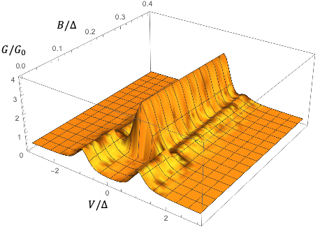
Both of these observations are in perfect alignment with the experiment. Specifically we see the right behavior of a sudden and steep jump of the conductor at close to the theoretical value of (perfect conductivity).
Numerical Simulations
For a numerical simulation of the system, a surface-state (SS) Green’s function (GF) approach is applied to describe surface-bulk mixing. The surface bulk mixing is assumed to be due to impurity scattering at a Matsubara frequency, , and strength, . The effective action is then averaged over disorder configurations within the Born approximation to derive the self-energy, . This self-energy term is then incorporated into the SSGF to obtain the gold surface-state effective Hamiltonian when in contact with EuS islands on vanadium under a magnetic field parallel to the surface:
| (5) |
where are the Pauli matrices that describe the particle-antiparticle pairs, is the spin, is the superconducting gap, is the exchange term, and is the spin-orbit coupling (SOC) term. Taken altogether, a Majorana bound state (MBS) at the edges of the gold nanowire are described by this model and can be probed by a scanning tunneling microscope (STM) in contact with the gold surface.
The conductance calculated from this effective Hamiltonian as a function bias voltage and its temperature and magnetic field dependence is in agreement with the analytical results. A representative figure of the magnetic field dependence is shown in Fig. 3


To elucidate the origin of the zero bias peak in conductance and the mechanism responsible for its emergence, a tight-binding approach is employed [26]. A multi-dimensional version of the time-independent Schrödinger equation (TISE) is put forth:
| (6) |
For the 2-D case, this equation parameterized with a single hopping parameter, and then discretized to the lattice structure, by a lattice constant , specified by the system in question:
| (7) | |||||
| (8) | |||||
| (9) | |||||
| (10) |
The algorithm is then implemented under the limit as with a discretized TISE including the on-site Hamiltonian with electron hopping in the x-direction and y-direction, such that the Hamiltonian describing the system is given by:
| (11) |
Hard-wall ’particle in a box’ confinement is achieved by limiting hopping beyond a certain spatial region and in empty lattice sites. With this approach, the conductance in a Kitaev chain is calculated to confirm the emergence of a zero bias peak, and shown in Fig. 4. The fact that the MBS behavior in this system may be modelled by tight-binding implies that the chemistry of the system in question, i.e. the EuS/Au/V junction, is negligible and the physics dominate the emergence of this phenomenon.


Noise Predictions
This study gives us confidence that we should be able to make a proper prediction for the noise as the second derivative of with respect to . We have plotted as a function of voltage and magnetic field, see Fig. 5.

We observe the noise following the behavior of the current meaning that the additional noise contribution decreases massively at below as this is the position of the Andreev bound states and where the system becomes normal conducting. This is the perfect reflection of for Andreev reflection. Above we see that the noise is rising as the system becomes more transparent and conducts better but the rise does not reflect the massive change in conductivity seen before. This is due to the fact that due to the perfect conductivity of the Majorana the usual Fano factor of 2 for Andreev reflection below the gap does not apply. This means that the noise is indeed a clear differentiator also for the parameters chosen in the experiment to differentiate a Majorana fermion from other possible effects leading to a steep rise in conductance below the superconductor gap.
Conclusion
We have analyzed the behavior of a superconducting system including a Majorana fermion theoretically in comparison to experimental data.
The study has given us confidence that the Hamiltonian formalism allows for a proper description of the system in question. It has also revealed the noise features of the system showing that the typical Fano factor of 2 should be drastically reduced for Andreev reflection off a Majorana fermion also for experimentally observable parameters.
This behavior can be measured experimentally using techniques previously employed for the study of normal-superconductor point contacts and there noise behavior.
References
- [1] Paul Adrien Maurice Dirac. Relativistic wave equations. Proceedings of the Royal Society of London. Series A-Mathematical and Physical Sciences, 155(886):447–459, 1936.
- [2] Ettore Majorana. Theory of the symmetry of electrons and positrons. Nuovo Cim, 14(171):50, 1937.
- [3] Meng Cheng, Roman M Lutchyn, and S Das Sarma. Topological protection of majorana qubits. Physical Review B, 85(16):165124, 2012.
- [4] Karsten Flensberg, Felix von Oppen, and Ady Stern. Engineered platforms for topological superconductivity and majorana zero modes. Nature Reviews Materials, 6(10):944–958, 2021.
- [5] CWJ Beenakker. Search for majorana fermions in superconductors. Annu. Rev. Condens. Matter Phys., 4(1):113–136, 2013.
- [6] Sujit Manna, Peng Wei, Yingming Xie, Kam Tuen Law, Patrick A Lee, and Jagadeesh S Moodera. Signature of a pair of majorana zero modes in superconducting gold surface states. Proceedings of the National Academy of Sciences, 117(16):8775–8782, 2020.
- [7] Peng Wei, Sujit Manna, Yingming Xie, Kam Tuen Law, Patrick Lee, and Jagadeesh Moodera. The demonstration of majorana zero modes in scalable gold nanowires. In Spintronics XIII, volume 11470, page 114700L. SPIE, 2020.
- [8] Steven R Elliott and Marcel Franz. Colloquium: Majorana fermions in nuclear, particle, and solid-state physics. Reviews of Modern Physics, 87(1):137, 2015.
- [9] Craig E Aalseth, N Abgrall, Estanislao Aguayo, SI Alvis, M Amman, Isaac J Arnquist, FT Avignone III, Henning O Back, Alexander S Barabash, PS Barbeau, et al. Search for neutrinoless double- decay in ge 76 with the majorana demonstrator. Physical review letters, 120(13):132502, 2018.
- [10] Hans Volker Klapdor-Kleingrothaus, A Dietz, L Baudis, G Heusser, IV Krivosheina, B Majorovits, H Paes, H Strecker, V Alexeev, A Balysh, et al. Latest results from the heidelberg-moscow double beta decay experiment. The European Physical Journal A-Hadrons and Nuclei, 12(2):147–154, 2001.
- [11] CE Aalseth, FT Avignone, RL Brodzinski, S Cebrian, D Gonzáles, E García, WK Hensley, IG Irastorza, IV Kirpichnikov, AA Klimenko, et al. Recent results of the igex 76ge double-beta decay experiment. Physics of Atomic Nuclei, 63(7):1225–1228, 2000.
- [12] HV Klapdor-Kleingrothaus, IV Krivosheina, A Dietz, and O Chkvorets. Search for neutrinoless double beta decay with enriched 76ge in gran sasso 1990–2003. Physics Letters B, 586(3-4):198–212, 2004.
- [13] N Abgrall, IJ Arnquist, FT Avignone III, AS Barabash, FE Bertrand, AW Bradley, V Brudanin, M Busch, M Buuck, J Caja, et al. The processing of enriched germanium for the majorana demonstrator and r&d for a next generation double-beta decay experiment. Nuclear Instruments and Methods in Physics Research Section A: Accelerators, Spectrometers, Detectors and Associated Equipment, 877:314–322, 2018.
- [14] Wenqin Xu, N Abgrall, FT Avignone, AS Barabash, FE Bertrand, V Brudanin, M Busch, M Buuck, D Byram, AS Caldwell, et al. The majorana demonstrator: a search for neutrinoless double-beta decay of 76ge. In Journal of Physics: Conference Series, volume 606, page 012004. IOP Publishing, 2015.
- [15] Vincente Guiseppe. New results from the majorana demonstrator experiment. In XXVIII International Conference on Neutrino Physics and Astrophysics, page 30, 2018.
- [16] GK Giovanetti, N Abgrall, Estanislao Aguayo, FT Avignone III, AS Barabash, FE Bertrand, M Boswell, V Brudanin, M Busch, D Byram, et al. A dark matter search with malbek. Physics Procedia, 61:77–84, 2015.
- [17] H Soller and A Komnik. Charge transfer statistics of transport through majorana bound states. Physica E: Low-dimensional Systems and Nanostructures, 63:99–104, 2014.
- [18] Saleem Al Dajani and Henning Soller. Noise as a probe for majorana fermion surface states, poster presentation. In Noise from Condensed Matter Physics to Quantum Technologies, ETTORE MAJORANA FOUNDATION AND CENTRE FOR SCIENTIFIC CULTURE, Erice, Italy, April 24-30, 2022.
- [19] A Yu Kitaev. Unpaired majorana fermions in quantum wires. Physics-uspekhi, 44(10S):131, 2001.
- [20] Gil Refael. Majorana fermions, Sep 2015.
- [21] Yuval Oreg, Gil Refael, and Felix Von Oppen. Helical liquids and majorana bound states in quantum wires. Physical review letters, 105(17):177002, 2010.
- [22] Berthold Jäck, Yonglong Xie, and Ali Yazdani. Detecting and distinguishing majorana zero modes with the scanning tunnelling microscope. Nature Reviews Physics, 3(8):541–554, 2021.
- [23] Henrik Bruus and Karsten Flensberg. Many-body quantum theory in condensed matter physics: an introduction. OUP Oxford, 2004.
- [24] Dong E Liu, Meng Cheng, and Roman M Lutchyn. Probing majorana physics in quantum-dot shot-noise experiments. Physical Review B, 91(8):081405, 2015.
- [25] Andreas Burtzlaff, Alexander Weismann, Mads Brandbyge, and Richard Berndt. Shot noise as a probe of spin-polarized transport through single atoms. Physical Review Letters, 114(1):016602, 2015.
- [26] Christoph W Groth, Michael Wimmer, Anton R Akhmerov, and Xavier Waintal. Kwant: a software package for quantum transport. New Journal of Physics, 16(6):063065, 2014.
- [27] Michał Papaj and Liang Fu. Creating majorana modes from segmented fermi surface. Nature communications, 12(1):1–7, 2021.
- [28] Jacob F Steiner and Felix von Oppen. Readout of majorana qubits. Physical Review Research, 2(3):033255, 2020.
- [29] Luuk Coopmans, Di Luo, Graham Kells, Bryan K Clark, and Juan Carrasquilla. Protocol discovery for the quantum control of majoranas by differentiable programming and natural evolution strategies. PRX Quantum, 2(2):020332, 2021.
- [30] D Davis, H Gutfreund, and WA Little. Proposed model of a high-temperature excitonic superconductor. Physical Review B, 13(11):4766, 1976.
- [31] WA Little. Criteria for the design of an excitonic superconductor. International Journal of Quantum Chemistry, 20(S15):545–554, 1981.
- [32] DL Miller, Myron Strongin, OF Kammerer, and BG Streetman. Experimental search for excitonic superconductivity. Physical Review B, 13(11):4834, 1976.
- [33] John Bardeen. Excitonic superconductivity? Journal of the Less Common Metals, 62:447–450, 1978.
- [34] JC Cuevas, A Martín-Rodero, and A Levy Yeyati. Hamiltonian approach to the transport properties of superconducting quantum point contacts. Physical Review B, 54(10):7366, 1996.
- [35] BA Muzykantskii and DE Khmelnitskii. Quantum shot noise in a normal-metal–superconductor point contact. Physical Review B, 50(6):3982, 1994.
- [36] Mark R Buitelaar, Wolfgang Belzig, Thomas Nussbaumer, B Babić, Christoph Bruder, and Christian Schönenberger. Multiple andreev reflections in a carbon nanotube quantum dot. Physical review letters, 91(5):057005, 2003.
- [37] Wolfgang Belzig and Yu V Nazarov. Full counting statistics of electron transfer between superconductors. Physical Review Letters, 87(19):197006, 2001.
- [38] AO Gogolin and A Komnik. Towards full counting statistics for the anderson impurity model. Physical Review B, 73(19):195301, 2006.