Lessons from the Mathematics of Two-Dimensional Euclidean Quantum Gravity

The path integral approach to Euclidean Quantum Gravity Gibbons_Action_1977; Gibbons_Euclidean_1993 aims at assigning a mathematical meaning to a functional integral of the form

where the integration is over all isometry classes $[g_{ab}]$ of Riemannian metrics $g_{ab}$ on a $d$-dimensional spacetime manifold $M$ with an appropriate action $S[g_{ab}]$, like the (Euclidean) Einstein–Hilbert action

It has the key advantage over the Feynman path integral of Lorentzian quantum gravity that, at least formally, the integrand is real and positive, allowing for an interpretation of $\mathcal{Z}$ as a partition function of a statistical system in which $e^{-S[g_{ab}]}$ takes on the role of the Boltzmann weight assigned to the geometry $[g_{ab}]$. Putting aside the matter of relating the two path integrals via a “Wick rotation”, it turns the problem of Euclidean quantum gravity into a question of probability theory: does there exist a suitable probability measure

on the space of geometries on $M$?

Needless to say, there are significant challenges on the way to answering this question. As with other (Euclidean) Quantum Field Theory any approximation scheme of the integral (1) will encounter both ultraviolet and infrared divergencies that have to be suitably regularized. The absence of a background geometry, peculiar to gravity, makes categorizing the field degrees of freedom by scale (and thus deciding which are infrared or ultraviolet) already a non-trivial affair, because a notion of scale necessarily involves the dynamical metric itself. In addition, since gravity is perturbatively non-renormalizable, one should be prepared to deal with metric degrees of freedom at short length scales (i.e. in the ultraviolet) that are strongly interacting. Based on this one may question whether the space of Riemannian metrics provides an arena general enough to host the sought-after probability measure, since many classical notions of Riemannian geometry (like curvature and geodesics) may be lost when the metric becomes too irregular, for instance if the metric tensor is non-differentiable or even distributional. It may thus be necessary to find an appropriate generalization of the Riemannian metric that can support such a measure. Finally, in constructing the measure one should overcome the issue that the Einstein–Hilbert action (for $d\geq 3$) is unbounded from below, suggesting that certain highly curved geometries will receive much higher Boltzmann weight than the classical Einstein solutions (known as conformal factor problem Gibbons_Path_1978; Mazur_path_1990).

A mathematically precise construction of the partition function has not been achieved yet for any manifold of dimension $d\geq 3$, but significant progress is reported elsewhere in the handbook. Notably, renormalization group methods Reuter_Nonperturbative_1998; Dou_running_1998; Reuter_Renormalization_2002 (see Reuter_Quantum_2019 for a thorough account) have found indications that Euclidean Quantum Gravity is asymptotically safe Weinberg_Ultraviolet_1979, meaning that it is renormalizable with an interacting fixed point in the ultraviolet. Lattice discretization approaches like Euclidean Dynamical Triangulations Boulatov_phase_1991; Ambjoern_Four_1992; Ambjoern_vacuum_1992; Agishtein_Three_1991 and Causal Dynamical Triangulations Ambjoern_Nonperturbative_2012; Loll_Quantum_2019 provide a complementary perspective based on numerical methods.

In this chapter, however, we focus on Euclidean Quantum Gravity on the two-dimensional sphere which admits a fully rigorous probabilistic interpretation. It has been long known in the physics literature that the partition function in two dimensions is susceptible to analytic computation from various starting points, including the lattice approaches via Dynamical Triangulations David_Planar_1985; Ambjorn_Diseases_1985; Kazakov_Critical_1985; Ambjoern_Multiloop_1990; Ambjorn_Quantum_1997 and matrix models Hooft_planar_1993; Brezin_Planar_1978; DiFrancesco_2D_1995 as well as conformal field theory approaches via Liouville field theory Polyakov1981; Knizhnik_Fractal_1988; David_Conformal_1988; Distler_Conformal_1989. The focus of this chapter, however, is on the developments in the mathematical literature in the last two decades that have put these computations on a rigorous footing and have culminated in an unambiguous construction of the probability measure (3) representing two-dimensional Euclidean quantum gravity.

Of course, it is a greatly simplified toy model compared to quantum gravity on more realistic four-dimensional manifolds, but one that is far from trivial and already requires us to depart from certain classical intuition coming from Riemannian geometry. It thus forms an important test bed for our mathematical methods and several lessons can be learned (at least on what not to take for granted when searching for higher-dimensional analogues).

One aspect which sets gravity in two dimensions apart from its higher-dimensional counterparts is that Einstein’s field equations in vacuum are trivial: every Riemannian metric is a solution when $\Lambda=0$ and none is when $\Lambda\neq 0$. This is tied to the fact that the curvature integral in the Einstein–Hilbert action (2) for $d=2$ is a topological invariant due to the Gauss–Bonnet formula, so fixing the manifold $M=S^{2}$ to be the 2-sphere the only dependence on the metric is through its total volume $\int_{S^{2}}\sqrt{g}$. The partition function (1) can therefore formally be recast as an ordinary integration over the volume $V$ of the canonical partition function $\mathcal{Z}_{V}$,

Since every geometry of volume $V$ receives the same Boltzmann weight, the probability measure of two-dimensional quantum gravity (at fixed volume) should amount to a suitable notion of sampling a metric on $S^{2}$ uniformly at random.

It is not at all obvious how to interpret this in the infinite-dimensional space of Riemannian geometries on $S^{2}$, but two-dimensional Euclidean Dynamical Triangulations (EDT) provides a natural lattice discretization David_Planar_1985; Ambjorn_Diseases_1985; Kazakov_Critical_1985; Ambjoern_Multiloop_1990; Ambjorn_Quantum_1997. Instead of considering the full set of Riemannian geometries on $S^{2}$, one restricts to the piece-wise flat geometries that can be assembled from a fixed number of equilateral Euclidean triangles of identical size. This introduces both an ultraviolet cutoff, by having a finite lattice spacing, and an infrared cutoff, by limiting the maximal diameter of the geometry. Since the set of geometries is now finite, one can easily select a uniform random metric by assigning equal probability to each. Then the hope is that this probability measure admits a well-defined continuum limit upon shrinking the triangles while increasing their number. We will review this limit, known as the Brownian sphere, in detail in the mathematical framework of random planar maps, where informally the building blocks are arbitrary regular (but mostly even-sided) polygons with unit side length.

Based on the extensive mathematical literature we can summarize some important lessons as follows:

• •

  The universality observed in enumeration formulas for planar maps can be understood combinatorially via the existence of bijections between maps and trees (Section 3).

• •

  The infrared cutoff in the probability measure can be consistently removed by considering the limit of random infinite planar maps in an appropriate topology, known as the local topology (Section 5). Often the random infinite geometry is easier to analyze than one of fixed finite size, for instance when studying explorations (Section 6).

• •

  The ultraviolet cutoff can be removed via a continuum limit in which the lattice spacing scales appropriately with the size of the random planar map (Section 4). The convergence takes place with respect to the Gromov–Hausdorff topology on the space of (compact) metric spaces (sets equipped with distance functions), which is significantly larger than the space of Riemannian geometries. The limit, known as the Brownian sphere, is a random metric space with the topology of $S^{2}$ and well-defined notion of geodesics, providing a precise realization of the probability measure in (3). However, it is not Riemannian as becomes apparent when examining its geodesics more closely (Section 4.5).

• •

  Removing both cutoffs naturally leads to a random metric space, known as the Brownian plane (Section 5), with exact scaling symmetry, in the sense that multiplying all distances by a positive constant does not change its distribution. Such a scale-invariant random geometry should be interpreted as realizing a fixed point of the renormalization group associated to Euclidean quantum gravity.

In the previous section we informally introduced discrete surfaces as two-dimensional Riemannian geometries that can be obtained from gluing together regular Euclidean polygons. But since we are interested in precise enumeration, it is important to choose the combinatorial representation in an unambiguous fashion.

A simple way to do so is to start with a finite set of regular polygons of unit side length and label the sides by integers $1,2,\ldots,2n$ in an arbitrary fashion. Given a matching of $\{1,\ldots,2n\}$, i.e. a partition of $\{1,\ldots,2n\}$ into pairs, one may construct a closed surface by gluing the $2n$ sides accordingly, see Fig. 1. More precisely, we assume that the polygons have an orientation and that their sides, also referred to as half-edges, are oriented in counterclockwise direction. We can then make the gluing operation unambiguous by requiring that pairs of half-edges are identified with opposite orientation. If the resulting geometry is connected, this gluing of polygons is called a map.

Observe that the $2n$ half-edges of a map are identified into a graph with $n$ edges (hence half-edges) that is embedded in a topological surface, which is necessarily orientable and determined by its genus. This brings us to an alternative definition of a map as a graph together with a proper embedding in a closed oriented surface, where by proper embedding we mean that the edges do not intersect themselves or other edges, except where they meet at vertices, and that the edges together delimit a collection of topological disks, called the faces of the map (which are nothing but the interiors of the polygons above). One then views two maps as equivalent if they can be related via an orientation-preserving homeomorphism of the surface. We should remark that graphs (and thus maps) are allowed to have more than one edge between a pair of vertices and to have edges starting and ending at the same vertex.

The sets of vertices, edges and faces of a map $\mathfrak{m}$ are denoted $\mathsf{V}(\mathfrak{m})$, $\mathsf{E}(\mathfrak{m})$ and $\mathsf{F}(\mathfrak{m})$ respectively. According to Euler’s formula, the numbers of vertices, edges and faces are related by

where $g$ is the genus of the corresponding surface. In the case $g=0$ we are dealing with a planar map, i.e. a polygonal gluing into a topological sphere or, equivalently, a planar graph properly embedded in the sphere. We take the degree of a vertex or face to be the number of edges incident to it (where we count an edge twice if both endpoints are at the same vertex or both sides adjacent to the same face). Special families of maps that we will encounter are triangulations¹¹ 1 In the literature these triangulations are sometimes called type I, because loops and multiple edges between vertices are allowed. Loopless triangulations, which forbid loops but allow multiple edges, are type II. Simple triangulations forbid both and are type III., quadrangulations, and even maps, whose faces all have degree three, degree four or even degree respectively. Even planar maps are also known as bipartite planar maps, because the vertices of such a map can be colored with two colors such that the endpoints of each edge have different color. This should be contrasted with the case of even maps of genus $g\geq 1$, which are not necessarily bipartite.

It should be observed that the polygonal gluing provides a highly redundant description of a map, since the half-edges carry an arbitrary labeling, whereas a description in terms of unlabeled embedded graphs is often too abstract to work with. This is especially true when the map in question possesses internal symmetries, i.e. when there exist orientation-preserving homeomorphisms of the sphere that non-trivially permute the edges and vertices of the map, called automorphisms. In such a case the number of labeled maps corresponding to the same unlabeled map $\mathfrak{m}$ is dependent on the size of the automorphism group $\operatorname{Aut}(\mathfrak{m})$ and is given by $(2n)!/|\operatorname{Aut}(\mathfrak{m})|$. A practical middle ground is to consider unlabeled but rooted maps, meaning that each map comes with a distinguished oriented edge (i.e. a distinguished half-edge). Sending a labeled map to the (unlabeled) rooted map obtained by distinguishing its half-edge with label $1$ is precisely $(2n-1)!$-to-$1$, so the enumeration of both types are more easily related to each other.

We are now ready to formulate in a precise combinatorial way the partition function of two-dimensional Euclidean Dynamical Triangulations (EDT) as a lattice discretization of the partition function (4). It can be defined as a summation over all unlabeled, labeled or rooted planar triangulations as

where $q_{3}$ can be interpreted as the exponential of the lattice cosmological constant and $T_{k}$ is the number of rooted planar triangulations with $2k$ triangles. In particular $3q_{3}Z_{\text{EDT}}^{\prime}(q_{3})=\sum_{k=1}^{\infty}q_{3}^{2k}T_{k}$ is nothing but the generating function of these numbers $T_{k}$, so its stands to reason that the enumeration of maps is at the heart of the model. If $q_{3}>0$ is small enough that the sum converges, the Boltzmann weights define a probability distribution on triangulations known as the Boltzmann triangulation. Furthermore, $T_{k}$ essentially is the corresponding canonical partition function of triangulations of fixed size $2k$, which therefore describes a random triangulation known as the uniform (rooted) triangulation of size $2k$, meaning that each rooted triangulation with $2k$ triangles occurs with equal probability $1/T_{k}$.

One may generalize this model to maps with faces of arbitrary degree by introducing a sequence of (non-negative) weights $\mathbf{q}=(q_{1},q_{2},q_{3},\ldots)$ and assigning those to the faces according to their degree as well as a weight $t>0$ to each vertex. Denoting the space of all rooted planar maps by $\mathcal{M}$, we are thus considering the partition function²² 2 Since the sum is over rooted planar maps, this partition function generalizes $3q_{3}Z_{\text{EDT}}^{\prime}(q_{3})$ rather than the partition function $Z_{\text{EDT}}(q_{3})$ of unlabeled triangulations.

If $Z(t,\mathbf{q})<\infty$, we can normalize the summand by $1/Z(t,\mathbf{q})$ and take it to define a probability distribution on $\mathcal{M}$, which is called the $(t,\mathbf{q})$-Boltzmann planar map. The parameter $t$ actually is redundant here, because by Euler’s formula (5) we have

meaning that the $(t,\mathbf{q})$-Boltzmann planar map is the same as the $\tilde{\mathbf{q}}$-Boltzmann planar map (with $t=1$). For combinatorial reasons it can be useful to keep the parameter $t$, while we will often set $t=1$ later without loss of generality.

We could have chosen to assign weights to the vertices depending on their degrees instead of the faces, but the resulting models are related by duality. Here the dual of a genus-$g$ map $\mathfrak{m}$ is the map $\mathfrak{m}^{\dagger}$ obtained by interchanging the roles of vertices and faces of $\mathfrak{m}$, while keeping the same incidence relations. More operationally, one places a vertex of $\mathfrak{m}^{\dagger}$ in each face of $\mathfrak{m}$ and one connects these by drawing an edge of $\mathfrak{m}^{\dagger}$ intersecting each edge of $\mathfrak{m}$. The root of $\mathfrak{m}^{\dagger}$ is taken to be the oriented edge starting at the root face and crossing the root of $\mathfrak{m}$. Since this is a bijection from $\mathcal{M}$ to itself and the vertex degrees of $\mathfrak{m}^{\dagger}$ agree with the face degrees of $\mathfrak{m}$, the dual of a $\mathbf{q}$-Boltzmann planar map is distributed according to the model with vertex weights. A hybrid version, in which both vertices and faces receive weights, poses significant additional challenges, and only limited progress has been made towards solving such models (see DiFrancesco1993; Kazakov1996; Kazakov1996a; Kazakov2022).

We start by recalling the classic approach to map enumeration initiated by Tutte in the sixties Tutte_Census_1962; Tutte_Census_1963; Tutte_enumeration_1968 and which is at the heart of the developments in the EDT (see Ambjorn_Quantum_1997 for an overview and Eynard2016; Ambjorn2022 for more recent accounts).

The central idea is that, while it is difficult to write an equation for the partition function itself, it is straightforward to obtain one for the generating function of maps with a boundary of controlled length. Here by boundary or root face (denoted $f_{\mathrm{r}}$) we simply mean the face that lies on the left of the root edge, and its degree is referred to as the perimeter of the map. One thus considers the disk generating function

where by convention we set $W^{(0)}(t,\mathbf{q})=t$, counting the map consisting of a single vertex and no edges. In the following we will drop the explicit dependence on $\mathbf{q}$ for notational simplicity and simply write $W^{(\ell)}$.

For any $\ell\geq 1$ one can decompose a rooted map by removing the root edge, which either leads to a map with one face less or to a pair of maps, see Fig. 2. At the level of generating functions this decomposition leads to the famous Tutte equation or loop equation Tutte_enumeration_1968

By introducing a generating variable $x$ for the boundary length $\ell$,

this equation can be seen to be equivalent to $W(x)^{2}-V^{\prime}(x)W(x)$ being analytic at $x=0$. More precisely, we have the identity

which is solved by

Here the sign in front of the square root is determined by the requirement that $xW(x)\to t$ as $x\to\infty$.

Let us for the moment assume that only finitely many weights are nonzero, such that $V^{\prime}(x)$ and $Q(x)$ are both polynomials. The results, however, can be shown to hold more generally, as we will see in Section 3, where we will be more careful about convergence issues. In the polynomial case one can make the one-cut assumption (or use Brown’s Theorem Brown_existence_1965) that the polynomial $V^{\prime}(x)^{2}-4Q(x)$ factorizes as

where the sign of $M(X)$ is chosen such that $V^{\prime}(x)/(xM(x))\to 1$ as $x\to\infty$. Hence,

The polynomial $M(x)$ as well as the endpoints $c_{\pm}=c_{\pm}(t,\mathbf{q})$ of the branch cut are then completely determined in terms of the weights $t$ and $\mathbf{q}$ by expanding the right-hand side around $x=\infty$ and imposing the condition $xW(x)\to t$ as $x\to\infty$.

This can be made more explicit by performing the Zhukovsky transformation Eynard2016

which is designed such that $W(x(z))$ becomes a Laurent polynomial in $z$ (i.e. a polynomial in $z$ and $1/z$),

The pair of functions $x(z),y(z)$ is known as the spectral curve of the model and plays an important role in topological recursion Eynard_Topological_2005; Eynard_Invariants_2007; Eynard2016, which relates generating functions of maps with multiple boundaries or higher genus to the disk function. Since we will stick to the planar case, we will not delve into this topic.

Note that under the transformation $z\to 1/z$ the first term in (18) is symmetric, $V^{\prime}(x(1/z))=V^{\prime}(x(z))$, while the second is antisymmetric, $y(z)=-y(1/z)$. Since $W(x(z))=t\frac{4}{c_{+}-c_{-}}z^{-1}+O(z^{-2})$, it follows that for any $p\geq 0$ we have

where the notation $[z^{k}]f(z)$ for a Laurent polynomial $f$ refers to the coefficient of $z^{k}$ in $f$. Hence

The equations $[z^{0}]W(x(z))=0$ and $[z^{-1}]W(x(z))=4t/(c_{+}-c_{-})$ then uniquely determine $c_{\pm}$ in terms of $\mathbf{q}$ and $t$.

The partition function (8) can be retrieved from $W^{(2)}$ by the observation that zipping open the root edge of a rooted map results bijectively in a rooted map with boundary of length $2$ and at least two faces. Hence

The expression (16) for the disk function already displays a degree of universality, in that the general structure is independent of the weights $\mathbf{q}$ and $t$. This universality becomes more explicit when one considers planar maps with a distinguished face of specified degree Ambjoern_Multiloop_1990; Ambjorn_Properties_1990; Ambjorn_Quantum_1997; Eynard_Topological_2005, whose generating functions depend only on $c_{\pm}$. Let us concentrate on the special case of planar maps with a distinguished vertex, which are also called pointed planar maps. The generating function $W_{\bullet}^{(\ell)}(t,\mathbf{q})$ is defined just like $W^{(\ell)}(t,\mathbf{q})$ in (10), except the sum runs over pointed planar maps and the distinguished vertex does not receive weight $t$. It should be clear that pointed and unpointed disk functions are related by a $t$-derivative,

Inserting (18) and applying the chain rule, while observing that $V^{\prime}(x)$ does not depend on the weight $t$, one finds the relation Eynard2016

Now one should observe that the right-hand side of

is a Laurent polynomial that is symmetric under $z\to 1/z$, while the left-hand side approaches $1$ when $z\to\infty$, because $xW_{\bullet}(x)\to 1$ as $x\to\infty$. Hence, the full Laurent polynomial must be identically equal to $1$. Inverting the Zhukovsky transformation then leads to the universal formula

If only $q_{2},q_{4},\ldots$ are nonzero, we are dealing with bipartite planar maps and the branch cut $[c_{-},c_{+}]$ becomes symmetric around $0$. For future reasons we introduce the notation

such that

From the last formula we deduce by series expansion around $x=\infty$ that

Note in particular that $W_{\bullet}^{(2)}=2R$. By removing the contribution $2t$ of the maps consisting of a single edge and zipping closed the boundary of the remaining maps, we obtain the generating function

for pointed bipartite planar maps. Equation (20) with $p=1$ and $[z^{-1}]W(x(z))=t/\sqrt{R}$ results in the explicit recursive equation

The simple form of this equation and the universal form of the pointed disk function $W_{\bullet}(z)$ have appeared rather miraculously. In the following sections we will give two explanations for this simplicity, a bijective approach involving combinatorial trees and a probabilistic approach involving a peeling exploration. As a bonus, both approaches provide insights into the geometry of the $\mathbf{q}$-Boltzmann maps.

In the last section we have seen that particularly pointed maps admit simple generating functions, so let us consider a rooted bipartite planar map $\mathfrak{m}$ with a distinguished vertex, that we call the origin. Naturally one may assign a label $\ell_{v}$ to each vertex $v\in\mathsf{V}(\mathfrak{m})$ by taking $\ell_{v}$ to be the graph distance along the edges of $\mathfrak{m}$ from $v$ to the origin (Fig. 3a). Because $\mathfrak{m}$ is bipartite, the labels at the endpoints of each edge differ exactly by $1$. For reasons that will become clear soon, let us restrict to the situation where the labels along the root edge of $\mathfrak{m}$ increase from its start to end. This is the case for exactly half of the maps, so by (29) these should be enumerated by $R-t$, for which we will deduce a bijective explanation.

The Bouttier–DiFrancesco–Guitter bijection (BDFG) provides an encoding of these maps in terms of so-called mobiles. A mobile is a tree $\mathfrak{t}$, i.e. a rooted planar map with only one face, with black vertices and integer-labeled white vertices satisfying the following properties (see Fig. 3d for an example):

1. (i)

   The two endpoints of each edge have different color.

2. (ii)

   The root edge starts at a white vertex with label $0$.

3. (iii)

   Around each black vertex, if a white neighbour has label $\ell$ then the next white neighbour in clockwise order around the black vertex must have label at least $\ell-1$.

The procedure to associate a mobile $\mathfrak{t}$ to $\mathfrak{m}$ is as follows:

1. 1.

   Let the vertices of $\mathfrak{m}$ be white and draw a new black vertex in each face of $\mathfrak{m}$ (Fig. 3c).

2. 2.

   For each edge $e$ of $\mathfrak{m}$, let $v$ be the endpoint of $e$ with the largest label. Draw a new edge starting at $v$ and ending on the black vertex within the face to the left of $e$ when facing $v$ (Fig. 3b). If $e$ is the root of $\mathfrak{m}$ we take the new edge to be the new root (oriented away from $v$).

3. 3.

   Remove all original edges of $\mathfrak{m}$ as well as the origin vertex (Fig. 3d).

4. 4.

   Shift all labels uniformly such that the root vertex receives label $0$.

Why does this procedure result in a mobile? The main feature of the construction is that $\mathfrak{t}$ cannot have any cycles. The explanation is that for any edge $e$ of $\mathfrak{m}$ one can find a curve, called the left-most geodesic, starting at (say, the midpoint of) $e$ and ending at the origin that does not intersect $\mathfrak{t}$. This immediately implies the impossibility of cycles in $\mathfrak{t}$, because every cycle in $\mathfrak{t}$ would enclose the origin on one side and at least one edge on the other side, contradicting the existence of a left-most geodesic path from that edge to the origin.

The left-most geodesic is constructed as follows (see the dashed curve in Fig. 3c for an example): denote the endpoints of $e$ by $v_{\ell}$ and $v_{\ell-1}$ with labels $\ell$ and $\ell-1$ respectively. The curve starts by traversing $e$ towards $v_{\ell-1}$. If $\ell=1$, $v_{\ell-1}$ is the origin and we are done. Otherwise, the curve circles around $v_{\ell-1}$ in clockwise direction until it encounters an edge with endpoint at distance $\ell-2$, that we denote $v_{\ell-2}$. Such an edge always exists due to the definition of the graph distance, and by construction of $\mathfrak{t}$ one encounters no edge of $\mathfrak{t}$ along the way. Traversing the edge to $v_{\ell-2}$ and iterating, one obtains a curve ending at the origin $v_{0}$, since that is the unique vertex with minimal label. The path $v_{\ell},v_{\ell-1},\ldots,v_{0}$ in $\mathfrak{m}$ is called the left-most geodesic, because it is a path of minimal length from $v_{\ell}$ to the origin and at each vertex it chooses the left-most option among such minimal paths.

In the absence of cycles, the number of connected components of $\mathfrak{t}$ is given by $|\mathsf{V}(\mathfrak{t})|-|\mathsf{E}(\mathfrak{t})|$. But by construction $|\mathsf{V}(\mathfrak{t})|=|\mathsf{V}(\mathfrak{m})|+|\mathsf{F}(\mathfrak{m})|-1$ and $|\mathsf{E}(\mathfrak{t})|=|\mathsf{E}(\mathfrak{m})|$, which together with Euler’s formula (5) implies that $\mathfrak{t}$ has a single connected component and is thus a tree. That the labels satisfy the properties of a mobile is straightforwardly checked from the construction.

Starting from a mobile $\mathfrak{t}$ one constructs a map $\mathfrak{m}$ in a reverse fashion. The angular region around a vertex $v$ that is delimited by two neighbouring edges incident to $v$ is called a corner of $v$. The contour of a face $f$ is the cyclic sequence of corners one encounters while walking around the perimeter of $f$ while keeping the edges on the right-hand side. The contour of (the unique face of) a tree thus visits all its corners in clockwise direction. The procedure is then as follows:

1. 1.

   Add a new white vertex (the origin) with label $\ell_{\mathrm{min}}-1$ in the face of $\mathfrak{t}$, where $\ell_{\mathrm{min}}$ is the minimal label of $\mathfrak{t}$.

2. 2.

   For each corner $c$ of a white vertex with label $\ell$ in $\mathfrak{t}$, we draw a new edge from $c$ to the next corner of a white vertex in the contour that has label $\ell-1$ in case $\ell>\ell_{\mathrm{min}}$ or to the origin in case $\ell=\ell_{\mathrm{min}}$. If $c$ is the corner of the root vertex that sits left of the root edge, then the new edge is taken to be the new root (oriented away from $c$).

3. 3.

   Remove all edges of $\mathfrak{t}$.

One can show BDFG04 that the construction is well-defined for any mobile, in the sense that the edges in the second step can be drawn unambiguously in a non-intersecting fashion, and that this is precisely the inverse of the construction in Section 3.2. Note that the labels of $\mathfrak{t}$ need to be shifted by $1-\ell_{\mathrm{min}}$ to arrive at the graph distances to the origin.

Let us make an observation about the left-most geodesics that will become important later LeGall_topological_2007. We have precisely one such geodesic $v_{\ell},v_{\ell-1},\ldots,v_{\ell_{\mathrm{min}}-1}$ of length $\ell-\ell_{\mathrm{min}}+1$ for each corner $c$ of a white vertex with label $\ell$ in $\mathfrak{t}$ and the path can be easily deduced from the sequence of labels in the contour of $\mathfrak{t}$: for $\ell_{\mathrm{min}}\leq i<\ell$ the vertex $v_{i}$ is simply the first vertex with label $i$ encountered when following the contour starting from $c$. In particular, two geodesics from corner $c$ at vertex $v$ and coner $c^{\prime}$ at vertex $v^{\prime}$ will typically merge before reaching the origin (see Fig. 3c). The merge happens at a vertex with label $\max(k,k^{\prime})-1$ where $k$ is the minimal label along the contour between $c$ (inclusive) and $c^{\prime}$ (exclusive), and $k^{\prime}$ is the minimal labels in the contour between $c^{\prime}$ (inclusive) and $c$ (exclusive). Although one cannot easily deduce the graph distance $d_{\mathrm{gr}}(v,v^{\prime})$, we do find an upper bound by concatenating the geodesics up to their merger,

In the BDFG bijection each face of $\mathfrak{m}$ of degree $2k$ corresponds to a black vertex in $\mathfrak{t}$ of degree $k$ and each vertex, except for the distinguished one, to a white vertex of $\mathfrak{t}$. As a consequence, the generating function $R(t,\mathbf{q})-t$ from (29) for (half of) the pointed bipartite planar maps is also the generating function of mobiles with at least one edge and a weight $t$ per white vertex and a weight $q_{2k}$ per black vertex of degree $k$. These mobiles admit a convenient recursive decomposition. Let us denote the root vertex by $v_{0}$. If the degree of the black vertex at the end of the root edge is $k$, then it has $k-1$ white children $v_{1},\ldots,v_{k-1}$. Each vertex $v_{i}$ together with its offspring, excluding the branch of the root edge in case of $v_{0}$, determines a mobile, once the labels have been shifted such that the root vertex $v_{i}$ receives label $0$. Noting that these mobiles may take the form of a single white vertex with no children, this leads immediately to the equation

because there are precisely $\binom{2k-1}{k}$ choices for the labels $\ell_{1},\cdots,\ell_{k-1}$ on $v_{1},\ldots,v_{k-1}$ satisfying the requirements $\ell_{1}\geq-1$, $\ell_{k}\leq 1$, and $\ell_{i+1}\geq\ell_{i}-1$ for $i=1,\ldots,k-1$. We thus reproduce equation (30). Since the summand gives the contribution of maps with root face of degree $2k$, we also reproduce

where the factor of $2$ compensates for the fact that only half of the edges adjacent to the root face have increasing label and can thus serve as root edge.

So far we have ignored issues of convergence in the computations of partition functions, which is ok if one chooses to work only at the level of formal generating series. However, soon we will be questioning the statistical properties of random maps, so we better make sure that the probability measures are sane. Luckily the tree bijections allow one to easily deduce criteria on the weight sequence $\mathbf{q}$. Restricting to non-pathological cases where at least one of $q_{4},q_{6},\ldots$ is non-zero, we say $\mathbf{q}$ is admissible when the generating function of rooted, pointed planar maps (with weight $t=1$ per vertex) is finite, $R(\mathbf{q})=R(t=1,\mathbf{q})<\infty$. This implies the same for (unpointed) rooted planar maps, $Z(\mathbf{q})<\infty$ and those with boundary, $W^{(2\ell)}(\mathbf{q})<\infty$ for all $\ell\geq 1$. With some extra work one can show that the converse is true as well Bernardi2019; Curien2019, namely that $Z(\mathbf{q})<\infty$ or $W^{(2\ell)}(\mathbf{q})<\infty$ for some $\ell\geq 1$ implies $R(\mathbf{q})<\infty$, so any of these criteria can be used as definition of admissibility.

From equation (32) it follows that a necessary condition for $\mathbf{q}$ to be admissible is that the equation

has at least one solution, since $g_{\mathbf{q}}(R)=1$ when $\mathbf{q}$ is admissible. It turns out that this is also sufficient and that $R(\mathbf{q})$ is given by the smallest positive fixed point Marckert2007. The reasoning is instructive, so we will summarize it here.

If $g_{\mathbf{q}}(r_{1})=1$ we have the identity

Since each term is positive, we may interpret them as probabilities and explicitly construct a random mobile as follows. We start with a single white node, that we designate to be active. Then at each step we visit each active white node and with probability $r_{1}^{-1}$ we deactivate the node or with probability $\binom{2k-1}{k}r_{1}^{k-1}$ we insert a black descendant which in turn has $k-1$ new active white descendants. The crux is to determine whether this random process produces a finite or an infinite tree. By adding up the probabilities of all finite mobiles thus produced, one finds that the mobile will be finite with probability

On the other hand, the number of active white nodes at each step in our construction has precisely the law of a Bienayme–Galton–Watson (BGW) process. It is well known that the probability of extinction of such a process is $1$ if and only if the mean offspring per individual is less or equal to $1$. In our case the mean offspring is $\sum_{k=1}^{\infty}k\,q_{2k}\binom{2k-1}{k}r_{1}^{k-1}=1-g_{\mathbf{q}}^{\prime}(r_{1})$. Since $g_{\mathbf{q}}(0)=0$ and $r_{1}$ is the first solution to $g_{\mathbf{q}}(r)=1$, we must have $g_{\mathbf{q}}^{\prime}(r_{1})\in[0,1)$. So the mean offspring is at most $1$, implying that the probability (36) equals $1$ and therefore $R(\mathbf{q})=r_{1}$. This verifies our claim.

This last observation naturally leads to a distinction between admissible sequences $\mathbf{q}$ that are subcritical, if $g_{\mathbf{q}}^{\prime}(R)>0$, and those that are critical, if $g_{\mathbf{q}}^{\prime}(R)=0$. To understand the difference, we can have a look at the generating function $R(t,\mathbf{q})$ that includes a weight $t\in[0,1]$ per vertex, which satisfies

The probability that a (unpointed but rooted) $\mathbf{q}$-Boltzmann map has precisely $n$ vertices is

For large $n$ this probability is thus determined by singularity analysis of $g_{\mathbf{q}}^{-1}$.

Let’s first focus on the case where $g_{\mathbf{q}}$ has radius of convergence larger than $R(\mathbf{q})$, in which case $\mathbf{q}$ is called regular. This happens for instance when only a finite number of weights $q_{2k}$ are non-zero. In the subcritical case $g_{\mathbf{q}}^{\prime}(R)>0$, we have that $g_{\mathbf{q}}^{-1}(t)$ has radius of convergence larger than $1$. Therefore the number of vertices has an exponential tail: there exists a $c>0$ such that for all $n\geq 0$,

In the critical case $g_{\mathbf{q}}^{\prime}(R)=0$ we necessarily have $g_{\mathbf{q}}^{\prime\prime}(R)<0$ and therefore $g_{\mathbf{q}}^{-1}(t)=R-\sqrt{\frac{1-t}{\frac{1}{2}|g_{\mathbf{q}}^{\prime\prime}(R)|}}+o(\sqrt{1-t})$. The same expansion applies to the more general case of generic critical $\mathbf{q}$, in which $g_{\mathbf{q}}$ is allowed to have a radius of convergence as small as $R(\mathbf{q})$, but for which $g_{\mathbf{q}}^{\prime\prime}(R)$ is still finite. Singularity analysis then implies that³³ 3 Here and in the following we will use the notation $f(n)\stackrel{{\scriptstyle n\to\infty}}{{\sim}}g(n)$ if $f(n)$ is asymptotic to $g(n)$ as $n\to\infty$, i.e. when $\lim_{n\to\infty}f(n)/g(n)=1$.

The string susceptibility exponent $\gamma_{\mathrm{s}}$ is thus a universal critical exponent for generic critical Boltzmann maps.

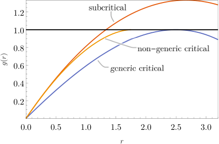
One may escape this universality only when $g_{\mathbf{q}}$ has radius of convergence exactly equal to $R(\mathbf{q})$ and $g_{\mathbf{q}}^{\prime\prime}(R)=-\infty$. In particular, $\mathbf{q}$ is called non-generic critical of type $a$ if LeGall_Scaling_2011; Budd_Geometry_2017; Ambjorn_Generalized_2016; Borot_recursive_2012

Observe that we need to take $a\in(3/2,5/2)$ to ensure $g_{\mathbf{q}}^{\prime}(R)=0$ and $g_{\mathbf{q}}^{\prime\prime}(R)=-\infty$. In this case $g_{\mathbf{q}}^{-1}(t)=R-(\frac{1}{C}(1-t))^{2/(2a-1)}+o\left((1-t)^{2/(2a-1)}\right)$ and therefore one finds

An example Ambjorn_Multi_2016; Budd_Geometry_2017 of such a non-generic critical weight sequence $\mathbf{q}$ of type $a\in(3/2,5/2)$ is

for which

In full generality it holds that an admissible sequence $\mathbf{q}$ is critical if and only if the number of vertices of a $\mathbf{q}$-Boltzmann planar map has infinite variance. Critical random maps are therefore much more likely to be very large than subcritical ones, making them the natural choice to investigate scaling limits. Perhaps more importantly, we will see later in Section 6.4 that critical random maps naturally occur within infinite maps.

Besides providing a combinatorial interpretation to the simple enumeration formulas for pointed maps, the tree bijection provides a natural way to study geodesic distances. To illustrate this, let us focus on the simplest example of quadrangulations, i.e. $q_{k}=q_{4}\delta_{k,4}$, referring the interested reader to Bouttier_Geodesic_2003 for the general case. From the previous discussion it easily follows that random quadrangulations are subcritical when $q_{4}<1/12$ and generic critical for $q_{4}=1/12$.

In the corresponding mobiles the black vertices all have degree two, meaning that we may as well merge the pair of edges adjacent to each black vertex to obtain a tree with white vertices only (Fig. 5). The labels between neighboring white vertices are then seen to differ by at most $1$, such that (32) becomes

This bijection between pointed quadrangulations and labeled trees is precisely the Cori–Vauqelin–Schaeffer bijection Cori_Planar_1981; Schaeffer_Conjugaison_1998. One can approach the enumeration of quadrangulations with control on geodesic distances Bouttier_Geodesic_2003 by introducing the generating function $R_{d}$ of quadrangulations in which the labels increase along the root edge and such that the start of the root edge has label at most $d$. Then $R_{0}=Z$, because for $d=0$ the origin must be located at the start of the root edge, and $\lim_{d\to\infty}R_{d}=R$, while

is the generating function of pointed quadrangulations in which the start and end of the root edge are at distance exactly $d$ and $d+1$ from the origin, respectively. The reason to work with $R_{d}$ instead of directly with $G_{d}$ is that $R_{d}$ satisfies a recursion equation that generalizes (45),

We can understand this equation by interpreting $R_{d}$ as the generating function of trees with positive integer labels that differ by at most $1$ between neighbors and such that the root vertex receives label $d+1$. Observing that the endpoint of the root edge has label $d$, $d+1$, or $d+2$ leads to the above formula.

Equation (47) can be solved explicitly Bouttier_Geodesic_2003, yielding

This exact expression allows us already to deduce some statistics concerning geodesic distances in large random quadrangulations. For instance, we can consider the situation where we condition a pointed critical quadrangulation $\mathfrak{m}$ to have its distance $d_{\bullet}(\mathfrak{m})$ between the root vertex and the origin to be exactly equal to $d$ and then ask about the distribution of the size of $\mathfrak{m}$. It satisfies

Inserting (46) and (48), one may check that to achieve a non-trivial limit one should scale $\lambda$ proportionally to $d^{-4}$ as $d\to\infty$.

Put differently, if we let $\lambda=\Lambda\epsilon^{2}$ for $\Lambda>0$ fixed and consider $|\mathsf{F}(\mathfrak{m})|\epsilon^{2}$ to be a rescaled area of $\mathfrak{m}$, then $R(\tfrac{1}{12}e^{-\Lambda\epsilon^{2}})=2-2\sqrt{\Lambda}\epsilon+O(\epsilon^{2})$ and $x(\tfrac{1}{12}e^{-\Lambda\epsilon^{2}})=1-\sqrt{6}\sqrt[4]{\Lambda}\sqrt{\epsilon}+O(\epsilon)$. Keeping $d\sqrt{3\epsilon/2}=D$ fixed while sending $d\to\infty$, leads to a non-trivial limit $x^{d}=e^{-2\sqrt[4]{\Lambda}D}+O(\sqrt{\epsilon})$. Hence

The right-hand side is known as the geodesic two-point function of two-dimensional quantum gravity with cosmological constant $\Lambda$, which was identified first by Ambjorn and Watabiki in Ambjorn_Scaling_1995. In particular,

which signals that typical geodesic distances in a quadrangulation with $n$ faces are of order $n^{1/4}$.

Recall that a metric space is a pair $(V,d)$ consisting of a set $V$ and a distance function $d:V\times V\to\mathbb{R}$ satisfying $d(x,x)=0$ for $x\in V$, $d(x,y)=d(y,x)>0$ when $x\neq y$ and the triangle inequality $d(x,z)\leq d(x,y)+d(y,z)$ for all $x,y,z\in V$. We denote the space of all compact metric spaces, viewed up to isometry, by $\mathbb{M}$. Note that this is a huge space: it contains all finite metric spaces, all metric spaces induced by compact Riemannian manifolds of arbitrary dimension and topology, but also much wilder spaces.