Newly identified compact hierarchical triple system candidates using Gaia DR3

As a result of our study, we have identified 403 hierarchical triple candidates among formerly known EBs from the literature based on the periods of their Gaia NSS orbital solutions. The first 35 candidates and the parameters of their corresponding Gaia NSS orbital solutions are listed in Table 4, while the full list will be available as an online table in CDS. There are 100 pure spectroscopic, 267 pure astrometric and 31 combined Gaia NSS solutions in our sample. There are also three objects with two separate astrometric and spectroscopic solutions along with two other objects with separate astrometric and combined solutions. For objects with two different types of orbital solutions, we chose to use the pure astrometric solution in every case as a convention. In Fig. 1 we illustrate the distribution of the inner and outer orbital periods (the periods of the corresponding NSS solutions) for all of our candidates. Broadly speaking, the outer periods range from somewhat greater than 1000 days, down to just a few days, though with the bulk of them concentrated between 300 and 1000 days. The sharp falloff in systems above $\sim$1000 days is an artefact of the Gaia observational window. The inner binary periods range from a fraction of a day to 10 days, simply representing the observational selection effects of the underlying EB catalogs that we utilized. Most of the longer outer periods are based on either a Gaia astrometric or spectroscopic solution, while essentially all of the outer orbits with periods less than $\sim$100 days are pure Gaia spectroscopic solutions. We also indicate our chosen limiting period ratio of $P_{\rm out}/P_{\rm in}=5$ with a dashed line. The closer a system is to this line, the tighter it is. We note that one point is below this limit for which we will give an explanation later in Sect. 4.1.

Prior to this study, there were some 400 known triple-star systems with outer periods $\lesssim 1000$ days, and only about 30 known with periods $\lesssim 200$ days. These systems are discussed and tabulated in Tokovinin 2018; Borkovits et al. 2016; Hajdu et al. 2019; Hajdu et al. 2022 and Fig. 1 of Borkovits et al. 2022. Thus, this study has the potential to substantially increase the number of known triple-star systems with measured outer orbits.

In Fig. 2 (upper panel) we show the differential eccentricity probability distribution for the 403 triple candidates that we have identified. The distribution is crudely described by the function

where $e$ is the outer eccentricity (see below for the origin of this functional form). This curve is superposed (after renormalization with the number of objects and the bin width) on the eccentricity distribution in Fig. 2, and provides a decent fit, considering the limited statistics. In the lower panel of Fig. 2 we show the cumulative probability distribution for the outer eccentricities that we have found. For comparison, we also show the eccentricity distributions for the Kepler sample of triples (Borkovits et al. 2016) and the outer orbits for 205 secure triples identified in the OGLE sample (Hajdu et al. 2019). In the same plot we compare these three empirical distributions with those of a flat eccentricity distribution ($dN/de=$ constant) and a so-called ‘thermal distribution’ ($dN/de\propto e$). It seems apparent that the empirical distributions are fairly similar to each other, but distinctly different from a differential distribution that is constant (linear as a cumulative distribution). And, for what it is worth, the empirical distributions are dramatically distinct from a thermal distribution, as suggested by Jeans 1919 for binary stellar systems which have reached a state of energy equipartition through a large series of dynamical encounters. In fact, the empirical distributions fairly closely resemble the empirical eccentricity distribution for ordinary binary stellar systems (Duchêne & Kraus 2013, see Fig. 3 of).

The cumulative eccentricity distribution for the Gaia-based outer eccentricity distribution can be reasonably well represented by the following analytic expression:

The derivative of this expression yields the above analytic approximation to the differential eccentricity distribution. There is one observational selection effect that we can envision for this data set in regard to the eccentricity distribution. That is, large eccentricities generally tend to make the triple star system more unstable. From Equation (16) of Rappaport et al. 2013 (Mikkola 2008; Mardling & Aarseth 2001, based on expressions for dynamical stability by),

we see that for period ratios of 1000, 300, 100, 30, and 10, the limiting eccentricities are $e=0.94;0.88;0.78;0.58$ and 0.28. Thus, one has to be somewhat careful about interpreting the relative dearth of high eccentricity systems.

In the sections below we discuss what we have done to try to validate the triple-star nature of some of these systems using ETV data. Additionally, as it turns out, some 27 of these systems were previously known triples or multiples (see Table 2). We also discuss the ‘truth probability’ for the SB1 solutions evaluated from the empirical formula of (Bashi et al. 2022). Thus, through these we acquire reasonable confidence that a substantial fraction (e.g., $\gtrsim 50\%$, and probably as high as 75%) of the new candidates are actually valid triple stars with a small fraction of quadruples. If this indeed turns out to be the case, then we will have substantially increased the number of known compact triple-star systems. If even half of our new candidates are proven to be valid triples, then this study will have increased the number of known compact triples by $\sim$1.5 times both below 1000 days and below 200 days. These compact triple systems, with RV orbits, third-body eclipses, and/or measurable dynamical interactions are the most likely multi-stellar systems to yield comprehensive measurements of all their stellar and orbital parameters. Here we hope to demonstrate by this project that finding Gaia outer orbits associated with known eclipsing binaries is a novel way to find new compact triples.

We checked the available publications in the literature for all single objects individually using SIMBAD (Wenger et al. 2000) and NASA ADS³³ 3 https://ui.adsabs.harvard.edu/. Most of these objects had not been involved in extensive studies apart from their identification as EBs. In Table 2, we have listed all 27 systems among our candidates for which we found any information about their possible triple star nature in the literature. Comparing the outer orbital periods from the Gaia solutions and the literature references, there are 14 objects (KIC 8330092, KIC 6525196, KIC 8043961, KIC 9665086, KIC 8719897, KIC 10991989, HD 181068, KIC 7955301, TIC 229785001, TIC 437230910, TIC 99013269, SAO 167450, HD 81919 and HD 190583) for which a reasonable agreement can be found. We consider these systems as validated candidates that are confirmed by the Gaia mission as an independent source. The only exception is SAO 167450, that is a visual member of AA Ceti in a bound EB+EB (2+2) hierarchical quadruple system, for which the Gaia spectroscopic orbital solution found belongs to one of the inner EBs and not to the outer orbit of the two EBs around their common center of mass.

For seven systems, although clear signs indicate that they have a multiple nature, their outer orbital period was unknown from previous studies. For V0857 Her, the presence of an additional component was suggested based on its rotational broadening function extracted from its spectra. For TIC 229082842 and TIC 59042291, an obvious sinusoidal variation was detected in their ETVs but the corresponding data sets were insufficient to derive their outer orbital periods. For TIC 305635022, signals of two eclipsing binaries were detected in its TESS LC that originate at the same pixels, hence it is a candidate 2+2 system. The remaining three objects, TIC 24704862, TIC 301956407 and TIC 410654298 are all subsystems of known visual double or multiple stars. In our opinion, the orbital solutions found by Gaia could also be considered as an independent confirmation of the multiple nature of these systems.

The rest of the six systems have significant differences between the two listed periods for them (Gaia vs. the literature). Two of them, although cataloged as EBs, are actually single stars with transiting exoplanets (TIC 438071843 and HATS-26). For these systems, it is possible that the Gaia orbital solutions belong to further stellar or exoplanet components on wider orbits. Finally, for the remaining four candidates, the ratios of the two periods (Gaia vs. the literature) are close to integers or half-integers that could indicate that at least one of the solutions over/underfitted the available sparse data for the same orbits, or it is also possible that the listed orbital periods belong to different components in these systems.

The observing strategy of TESS strongly limits the available data for objects, as most of them are observed only once or twice over $\sim$27 day long time-windows within a TESS Year, but objects closer to the ecliptic poles can have more overlapping Sectors with better data coverage with up to a year long quasi-continuous window. Moreover, the same hemispheres are only observed every other year, hence an apparent one-year long gap will appear even in the data set of the most well-observed objects. This means that our candidates also suffer from these observational effects and as a result we could not confirm the triple nature of all of them even if they show significant non-linear ETVs.

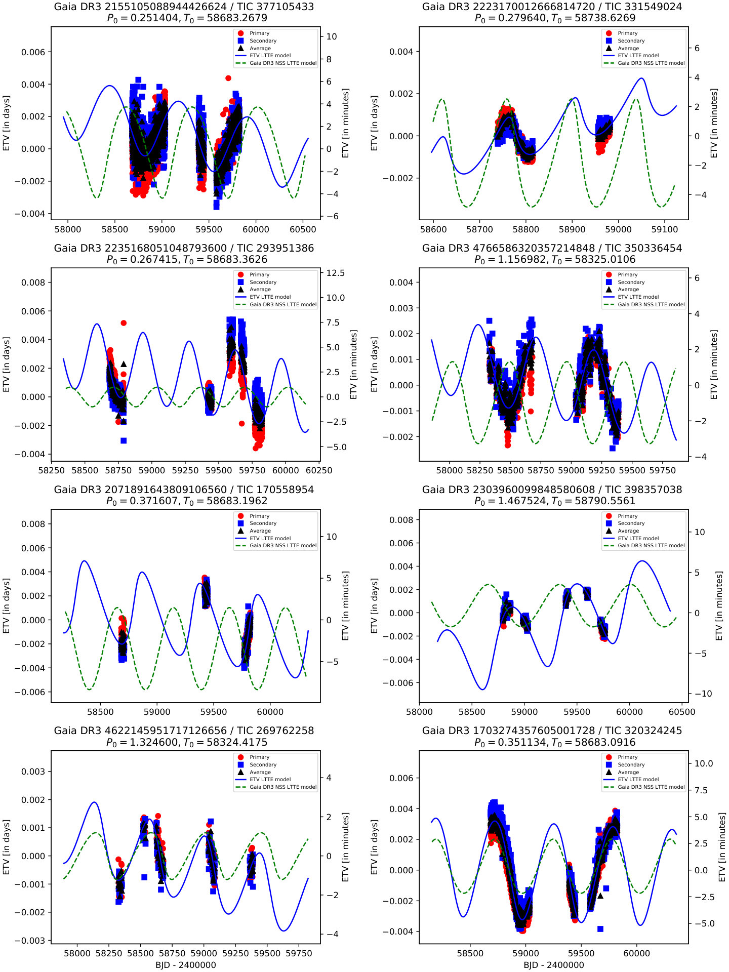
Nevertheless, we found 22 candidates that have sufficient data coverage, so that their ETVs can be reliably modeled with a simple LTTE solution. We plot the ETVs and the corresponding simple LTTE solutions using the Gaia and our own adjusted parameters for two of them in Fig. 3 as examples, while the rest of them can be found in Figs. 7, 8 and 9 in the Appendix. The corresponding model parameters can be found in Table 6.

As one can see in Fig. 3 (and the other such figures in the Appendix), the most noticeable thing is that the LTTE models calculated with the parameters of the Gaia orbital solutions can have either the same argument of periastron ($\omega_{NSS}=\omega_{ETV}$) or be 180 degrees away ($\omega_{NSS}=\omega_{ETV}\pm 180\degr$) from the LTTE models coming from our modeling process. This is not an error, and the reason for this is that the ETVs calculated from the TESS eclipses are always tracking the motion of the EB around the center of mass of the triple system, while for Gaia, this case is not so simple. For the astrometric solutions, Gaia uses the variations in the position in the photocenter of the object, while for spectroscopic solutions, it uses the variations in one or two detected peaks (for SB1 and SB2 solutions, respectively) in the cross-correlation function (CCF). This means that without the ETV solutions (or in the case of spectroscopic solutions, the CCFs) it is not straightforward to say which component of the triple system is tracked by Gaia.

In order to compare the orbital parameters of the Gaia NSS and our own ETV solutions, we plot their correlations in Fig. 4. On the top left panel, the two kinds of orbital periods are seen to be almost perfectly aligned with the line that represents a ratio of unity. That means Gaia found the outer orbital periods of these triples almost perfectly. On the top right panel, the projected semi-major axis of the different solutions are compared and it can be seen that for this parameter, the relation is far from perfect. Only a handful of objects can be found near the line of unity, and almost all are more or less above this line. This could arise from two reasons related to the nature of the astrometric solutions: i) for the majority of triple system parameters, the photocenter revolves around a smaller orbit, hence the semi-major axis of the outer orbit will be underestimated (Rappaport et al. 2022, see Eq. C2 of); ii) the ETV solutions can overestimate the semi-major axis if the orbits are not completely covered. However, for spectroscopic solutions, we cannot really say anything certain without reviewing the individual spectra⁷⁷ 7 These are not published in Gaia DR3. and the corresponding CCFs. In particular, the Gaia semi-major axis will depend on which component of the triple is being followed – in which case the sign of the discrepancy could go either way. The bottom left panel shows the relation of the eccentricities from the different solutions. Most points are in an agreement within the uncertainties, however, for the majority of the solutions, the error bars are quite large. As there are a high number of ETV solutions in which only a limited part of the orbit is covered, in those cases the orbit can be fitted equally well with a relatively wide range of eccentricities that results in larger uncertainties. Finally, on the bottom right panel, the arguments of periastron of the two solutions are compared to each other and those are grouped along two lines as expected. Those systems in which Gaia tracks the motion of the EB component (indicated with circles around them) are aligned with the yellow dashed line representing unity, while systems in which the tertiary component is tracked are aligned with the other, green dashed line. In conclusion, out of the 22 objects with the best-sampled TESS ETVs, one can state that, for triple candidates, the most reliable parameter from the Gaia orbital solutions is the outer orbital period and the outer eccentricity (although with higher uncertainties), while the other parameters should be used with caution, and only after identifying which component of the system is actually tracked by Gaia.

We also found four additional systems (TIC 66893949, TIC 298714297, TIC 88206187 and TIC 14839347) that show outer orbit third-body eclipses which inherently confirms the triple nature of these objects. First, we checked the FFIs of the corresponding objects and the extra eclipse events originate from the same pixels as the regular inner binary eclipses. Moreover, we also found evidence in archival ASAS-SN, ATLAS (Tonry et al. 2018; Smith et al. 2020) and WASP (Butters et al. 2010) photometric data that these objects are indeed triply eclipsing triple systems. The comprehensive photodynamical analysis of these newly discovered systems will be presented in a dedicated paper in the near future. Moreover, we also identified four additional systems (TIC 457671987, TIC 224053059, TIC 376606423 and TIC 410654298) that are most likely previously unknown EB+EB quadruples according to their TESS LCs. Nevertheless, we do not consider them as validated systems because although the signal of both EBs for these objects comes from the same pixels that does not necessary confirm that they are certainly bound in the same system. In particular, the two EBs could just be seen in the same direction without any direct physical connection between them.

We would like to highlight the special case of TIC 410654298 here which is the only object we kept although the ratio of the Gaia and the EB period is a bit less than 5. This object is cataloged with a $\sim$20 day EB period and there are two separate types of Gaia NSS solutions (astrometric and combined astrometric+spectroscopic) available for it with a similar period of $\sim$170 day. These resulted in a period ratio above 5 in the beginning. Nevertheless, after analyzing its TESS LC, we found that its actual EB period is $\sim$36.4 day which yields a period ratio below our chosen limit. However, as there are two different types of Gaia NSS solutions available for this systems, we would assume that the orbit found by Gaia is valid. A plausible explanation for this object could be that it is a 2+2 system with an eclipsing and a non-eclipsing component, and Gaia found the inner orbit of the latter, hence the 170 day period would not correspond to the outer orbit of the two binaries around the center of mass of the quadruple system.

There are 192 objects that show significant non-linear ETVs, but only a very short part of their outer orbit is covered by TESS observations, hence they cannot be fitted reliably with a simple LTTE model. Although the LTTE models calculated with the parameters from the Gaia orbital solutions do not perfectly match the observed ETVs, they are at least in accordance regarding the outer orbital periods for most of these systems. These systems also demonstrate that the most trustworthy parameter from the Gaia NSS solutions is the orbital period. We plotted two systems in Fig. 5 as an example to illustrate how the duration of available observational data compares to the typical outer orbital solutions. As non-linear ETVs are apparent in these systems, we also consider these systems as confirmed hierarchical triple systems, nevertheless we could not validate their outer orbital parameters from the Gaia NSS solutions.

Finally, the remaining 158 systems (403 total minus 245 that are validated in one way or another) either do not have any or a sufficient amount of TESS observations available, or their ETV curves do not show any non-linear behavior. In the absence of supplemental data, we could not confirm the triple nature of these systems, hence we consider them still as ‘candidates’ that should be studied in the future when a sufficient amount of high-quality photometric (or spectroscopic) observations become available for them.

The shortest outer period CHT currently known is $\lambda$ Tau with a 33 day outer orbital period (Ebbighausen & Struve 1956). As can be seen in our Fig. 1, there are some 30 candidates with periods under 35 days. Empirically, such systems should be very rare, so it is somewhat surprising that a significant number of our systems could belong to this category. However, it is hard to confirm the true nature of these systems using only TESS LCs and ETVs calculated from them. The amplitude of the LTTE depends on the semi-major axis which is obviously small for such systems, while the dynamical delays are proportional to the outer eccentricity which is also expected to be small according to formation scenarios, hence the amplitude of the ETVs of such systems are expected to be very small, within the order of our uncertainties. A further difficulty is that there is a very limited amount (or lack) of TESS observations of these systems.

High-resolution spectroscopy with good temporal coverage could be of help in revealing the true configurations of these objects, however, that is not available for now as Gaia DR3 contains only an average of all spectra for each object. Nevertheless, Bashi et al. 2022, based on the spectroscopic observations of known EBs by LAMOST and GALAH, determined an empirical formula that can estimate the probability that a Gaia spectroscopic SB1 solution is valid. We plot the period distribution of all 92 of our SB1-type candidates along with their empirical ‘truth probabilities’ in Fig. 6. For 64 and 36 systems this probability is at least 50% and 75%, respectively. In general, it can be seen that the longer the outer period the more probable the solution is valid. This means that among the candidates with short outer periods, we expect there to be several invalid solutions. Also, there is a possibility that if the Gaia orbital solution is valid, the object is actually a quadruple system with a 2+2 configuration with an eclipsing and a non-eclipsing binary component, and Gaia actually found the spectroscopic orbital solution of the non-eclipsing binary component (see the case of SAO 167450 in Sect. 3.2 and Table 2). However, for now, we cannot confirm or reject these candidates with certainty, because of insufficient supplemental observational data.

References

Babusiaux et al. (2022)
Babusiaux, C., Fabricius, C., Khanna, S., et al. 2022, arXiv e-prints,
arXiv:2206.05989
Bashi et al. (2022)
Bashi, D., Shahaf, S., Mazeh, T., et al. 2022, arXiv e-prints,
arXiv:2207.08832
Borkovits (2022)
Borkovits, T. 2022, Galaxies, 10, 9
Borkovits et al. (2013)
Borkovits, T., Derekas, A., Kiss, L. L., et al. 2013, MNRAS, 428, 1656
Borkovits et al. (2016)
Borkovits, T., Hajdu, T., Sztakovics, J., et al. 2016, MNRAS, 455,
4136
Borkovits et al. (2022)
Borkovits, T., Mitnyan, T., Rappaport, S. A., et al. 2022, MNRAS, 510,
1352
Borkovits et al. (2015)
Borkovits, T., Rappaport, S., Hajdu, T., & Sztakovics, J. 2015,
MNRAS, 448, 946
Brasseur et al. (2019)
Brasseur, C. E., Phillip, C., Fleming, S. W., Mullally, S. E., &
White, R. L. 2019, Astrocut: Tools for creating cutouts of TESS images
Butters et al. (2010)
Butters, O. W., West, R. G., Anderson, D. R., et al. 2010, A&A, 520,
L10
Conroy et al. (2014)
Conroy, K. E., Prša, A., Stassun, K. G., et al. 2014, AJ, 147,
45
Derekas et al. (2011)
Derekas, A., Kiss, L. L., Borkovits, T., et al. 2011, Science, 332, 216
Duchêne & Kraus (2013)
Duchêne, G. & Kraus, A. 2013, ARA&A, 51, 269
Ebbighausen & Struve (1956)
Ebbighausen, E. G. & Struve, O. 1956, ApJ, 124, 507
Espinoza et al. (2016)
Espinoza, N., Bayliss, D., Hartman, J. D., et al. 2016, AJ, 152, 108
Fekel & Willmarth (2009)
Fekel, F. C. & Willmarth, D. W. 2009, PASP, 121, 1359
Foreman-Mackey et al. (2013)
Foreman-Mackey, D., Hogg, D. W., Lang, D., & Goodman, J. 2013, PASP,
125, 306
Gaia Collaboration et al. (2016)
Gaia Collaboration, Prusti, T., de Bruijne, J. H. J., et al. 2016,
A&A, 595, A1
Gaia Collaboration et al. (2022)
Gaia Collaboration, Vallenari, A., Brown, A. G. A., et al. 2022, arXiv
e-prints, arXiv:2208.00211
Ginsburg et al. (2019)
Ginsburg, A., Sipőcz, B. M., Brasseur, C. E., et al. 2019, AJ,
157, 98
Griffin (2006)
Griffin, R. F. 2006, MNRAS, 371, 1159
Gürol & Müyesseroğlu (2005)
Gürol, B. & Müyesseroğlu, Z. 2005, Astronomische
Nachrichten, 326, 43
Hajdu et al. (2022)
Hajdu, T., Borkovits, T., Forgács-Dajka, E., Sztakovics, J., &
Bódi, A. 2022, MNRAS, 509, 246
Hajdu et al. (2019)
Hajdu, T., Borkovits, T., Forgács-Dajka, E., et al. 2019, MNRAS,
485, 2562
Halbwachs et al. (2022)
Halbwachs, J.-L., Pourbaix, D., Arenou, F., et al. 2022, arXiv
e-prints, arXiv:2206.05726
Hippke et al. (2019)
Hippke, M., David, T. J., Mulders, G. D., & Heller, R. 2019, AJ, 158,
143
Huang et al. (2021)
Huang, H.-P., Yu, Y.-X., Yu, T., Hu, K., & Xiang, F.-Y. 2021,
Research in Astronomy and Astrophysics, 21, 120
Innes (1895)
Innes, R. T. A. 1895, MNRAS, 55, 312
Jeans (1919)
Jeans, J. H. 1919, Nature, 103, 64
Kirk et al. (2016)
Kirk, B., Conroy, K., Prša, A., et al. 2016, AJ, 151, 68
Kristiansen et al. (2022)
Kristiansen, M. H. K., Rappaport, S. A., Vanderburg, A. M., et al.
2022, PASP, 134, 074401
Kushnir et al. (2013)
Kushnir, D., Katz, B., Dong, S., Livne, E., & Fernández, R.
2013, ApJ, 778, L37
Lightkurve Collaboration et al. (2018)
Lightkurve Collaboration, Cardoso, J. V. d. M., Hedges, C., et al.
2018, Lightkurve: Kepler and TESS time series analysis in Python,
Astrophysics Source Code Library
Lohr et al. (2015)
Lohr, M. E., Norton, A. J., Payne, S. G., West, R. G., & Wheatley,
P. J. 2015, A&A, 578, A136
Lu et al. (2001)
Lu, W., Rucinski, S. M., & Ogłoza, W. 2001, AJ, 122, 402
Luyten (1955)
Luyten, W. J. 1955, Luyten’s Five Tenths. (1955, 0
Mardling & Aarseth (2001)
Mardling, R. A. & Aarseth, S. J. 2001, MNRAS, 321, 398
Mason et al. (2001)
Mason, B. D., Wycoff, G. L., Hartkopf, W. I., Douglass, G. G., &
Worley, C. E. 2001, AJ, 122, 3466
Mikkola (2008)
Mikkola, S. 2008, in Multiple Stars Across the H-R Diagram, ed. S. Hubrig,
M. Petr-Gotzens, & A. Tokovinin, 11
Mitnyan et al. (2020)
Mitnyan, T., Borkovits, T., Rappaport, S. A., Pál, A., & Maxted,
P. F. L. 2020, MNRAS, 498, 6034
Munari et al. (2014)
Munari, U., Henden, A., Frigo, A., et al. 2014, AJ, 148, 81
Pál (2012)
Pál, A. 2012, MNRAS, 421, 1825
Pourbaix et al. (2022)
Pourbaix, D., Arenou, F., Gavras, P., et al. 2022, Gaia DR3
documentation Chapter 7: Non-single stars, Gaia DR3 documentation, European
Space Agency; Gaia Data Processing and Analysis Consortium. Online at ¡A
href=“https://gea.esac.esa.int/archive/documentation/GDR3/index.html”¿https://gea.esac.esa.int/archive/documentation/GDR3/index.html¡/A¿,
id. 7
Pourbaix et al. (2004)
Pourbaix, D., Tokovinin, A. A., Batten, A. H., et al. 2004, A&A, 424,
727
Pribulla et al. (2009)
Pribulla, T., Rucinski, S. M., Blake, R. M., et al. 2009, AJ, 137,
3655
Prša et al. (2022)
Prša, A., Kochoska, A., Conroy, K. E., et al. 2022, ApJS, 258,
16
Qian et al. (2008)
Qian, S. B., He, J. J., Soonthornthum, B., et al. 2008, AJ, 136, 1940
Qian et al. (2006)
Qian, S. B., Liao, W. P., He, J. J., Yuan, J. Z., & Zhu, L. Y. 2006,
New A, 12, 33
Rappaport et al. (2013)
Rappaport, S., Deck, K., Levine, A., et al. 2013, ApJ, 768, 33
Rappaport et al. (2022)
Rappaport, S. A., Borkovits, T., Gagliano, R., et al. 2022, MNRAS,
513, 4341
Riello et al. (2021)
Riello, M., De Angeli, F., Evans, D. W., et al. 2021, A&A, 649, A3
Rowan et al. (2022)
Rowan, D. M., Jayasinghe, T., Stanek, K. Z., et al. 2022, arXiv
e-prints, arXiv:2205.05687
Samus’ et al. (2017)
Samus’, N. N., Kazarovets, E. V., Durlevich, O. V., Kireeva, N. N., &
Pastukhova, E. N. 2017, Astronomy Reports, 61, 80
Shappee et al. (2014)
Shappee, B. J., Prieto, J. L., Grupe, D., et al. 2014, ApJ, 788, 48
Smith et al. (2020)
Smith, K. W., Smartt, S. J., Young, D. R., et al. 2020, PASP, 132,
085002
Taylor (2005)
Taylor, M. B. 2005, in Astronomical Society of the Pacific Conference Series,
Vol. 347, Astronomical Data Analysis Software and Systems XIV, ed.
P. Shopbell, M. Britton, & R. Ebert, 29
The Astropy Collaboration et al. (2018)
The Astropy Collaboration, Price-Whelan, A. M., Sipőcz, B. M.,
et al. 2018, AJ, 156, 123
Tokovinin (2014)
Tokovinin, A. 2014, AJ, 147, 87
Tokovinin (2018)
Tokovinin, A. 2018, ApJS, 235, 6
Tokovinin (2019)
Tokovinin, A. 2019, AJ, 158, 222
Tokovinin (2021)
Tokovinin, A. 2021, Universe, 7, 352
Tokovinin (1997)
Tokovinin, A. A. 1997, A&AS, 124, 75
Tonry et al. (2018)
Tonry, J. L., Denneau, L., Heinze, A. N., et al. 2018, PASP, 130,
064505
Toonen et al. (2022)
Toonen, S., Boekholt, T. C. N., & Portegies Zwart, S. 2022, A&A, 661,
A61
Toonen et al. (2020)
Toonen, S., Portegies Zwart, S., Hamers, A. S., & Bandopadhyay, D.
2020, A&A, 640, A16
Triaud et al. (2017)
Triaud, A. H. M. J., Martin, D. V., Ségransan, D., et al. 2017,
A&A, 608, A129
van den Bos (1921)
van den Bos, W. H. 1921, MNRAS, 81, 474
Vanderburg et al. (2016)
Vanderburg, A., Latham, D. W., Buchhave, L. A., et al. 2016, ApJS,
222, 14
Wang et al. (2015)
Wang, J. J., Qian, S. B., Zhang, Y. P., et al. 2015, AJ, 149, 164
Watson et al. (2006)
Watson, C. L., Henden, A. A., & Price, A. 2006, Society for Astronomical
Sciences Annual Symposium, 25, 47
Wenger et al. (2000)
Wenger, M., Ochsenbein, F., Egret, D., et al. 2000, A&AS, 143, 9
Yang et al. (2013)
Yang, Y. G., Qian, S. B., & Dai, H. F. 2013, AJ, 145, 60
Zasche et al. (2022)
Zasche, P., Henzl, Z., & Masek, M. 2022, arXiv e-prints,
arXiv:2205.03934
Appendix A Additional tables and figures