A sparsity-promoting resolvent analysis for the identification of spatiotemporally-localized amplification mechanisms

We start by considering a dynamical system of the form

$$\dot{\boldsymbol{x}}+\boldsymbol{A}\boldsymbol{x}=\boldsymbol{f},$$

(1)

with $\boldsymbol{x}$, $\boldsymbol{f}\in\mathbb{R}^{n}$, and $\boldsymbol{A}\in\mathbb{R}^{n\times n}$. Here, $\boldsymbol{A}$ is a linear operator, $\boldsymbol{x}$ represents the state of the system, and the term $\boldsymbol{f}$ represents an external input, which could come from neglected nonlinear terms. In this subsection, we proceed by taking a Fourier transform in time, thus considering solutions for both the state of the system and the forcing terms that are of the form.

$$\boldsymbol{x}=\hat{\boldsymbol{x}}\exp{(-i\omega t)},$$

(2)

$$\boldsymbol{f}=\hat{\boldsymbol{f}}\exp{(-i\omega t)},$$

(3)

with $\omega\in\mathbb{C}$ denoting the temporal frequency. Substituting Eqs. (2)-(3) into Eq. (1) gives

$$(-i\omega\boldsymbol{I}+\boldsymbol{A})\hat{\boldsymbol{x}}=\hat{\boldsymbol{f}}.$$

(4)

In the case where $i\omega$ is not in the spectrum of the operator $\boldsymbol{A}$, this equation can be recast as

$$\hat{\boldsymbol{x}}=(-i\omega\boldsymbol{I}+\boldsymbol{A})^{-1}\hat{\boldsymbol{f}}:=\mathcal{H}_{\omega}\hat{\boldsymbol{f}},$$

(5)

for which an arbitrary external forcing $\hat{\boldsymbol{f}}$ is mapped to a given state $\hat{\boldsymbol{x}}$ via the resolvent operator $\mathcal{H}_{\omega}$, defined at a given frequency, $\omega$.

In this work, we are interested in identifying cases where a forcing of a small magnitude $\hat{\boldsymbol{f}}$ produces a greatly amplified response $\hat{\boldsymbol{x}}$. This can be achieved through a pseudospectral analysis of the resolvent operator $\mathcal{H}_{\omega}$, through the singular value decomposition (SVD)

$$\mathcal{H}_{\omega}=\sum_{j=1}^{N}\psi_{j}\sigma_{j}\phi_{j}^{*},$$

(6)

where $(\cdot^{*})$ denotes the adjoint. In this decomposition, the singular values are sorted by decreasing energy content, such that $\sigma_{k}\geq\sigma_{k+1}\geq 0$ for all $k$. Additionally, the leading singular value and vectors are solutions to the following optimization problems

	$\displaystyle\sigma_{1}$	$\displaystyle=\max_{\|\phi\|=1}\|\mathcal{H}_{\omega}\phi\|=\max_{\|\psi\|=1}\|\mathcal{H}^{*}_{\omega}\psi\|,$		(7)
	$\displaystyle\phi_{1}$	$\displaystyle=\argmax_{\|\phi\|=1}||\mathcal{H}_{\omega}\phi||,$		(8)
	$\displaystyle\psi_{1}$	$\displaystyle=\sigma_{1}^{-1}\mathcal{H}_{\omega}\phi_{1}=\argmax_{\|\psi\|=1}||\mathcal{H}^{*}_{\omega}\psi||.$		(9)

Here, we formulate the resolvent operator for the nondimensionalized incompressible Navier-Stokes equations

$$\frac{\partial\boldsymbol{u}}{\partial t}+(\boldsymbol{u}\cdot\nabla)\boldsymbol{u}=-\nabla p+\frac{1}{Re}\Delta\boldsymbol{u},$$

(10)

$$\nabla\cdot\boldsymbol{u}=0,$$

(11)

where $\boldsymbol{u}=(u,v,w)$ is the velocity field, and $p$ is the pressure. When laminar base flows are considered, these equations are nondimensionalized based on the channel half-height, $h$, and the maximum streamwise flow speed, $U_{0}$. The Reynolds number is thus $Re=hU_{0}/\nu$, where $\nu$ is the kinematic viscosity. For turbulent flow, velocity is instead nondimensionalized using the friction velocity $u_{\tau}=\sqrt{\tau_{w}/\rho}$, with $\tau_{w}$ denoting the wall shear stress, and $\rho$ the fluid density. In the turbulent case, we thus use the friction Reynolds number $Re_{\tau}=hu_{\tau}/\nu$ in Eq.( 10). This system of equations is expressed in the form of Eqs. (1)-(5) by linearizing about either a laminar equilibrium or turbulent mean flow.

In this study we consider wall-bounded parallel flows with a unidirectional mean/base flow. This makes it convenient to formulate Eq. (5) in terms of the wall-normal velocity, $v$, and vorticity, $\eta=\partial u/\partial z-\partial w/\partial x$, Assuming Fourier transforms in the streamwise and spanwise directions with wavenumbers $k_{x}$ and $k_{z}$ respectively, this gives

$$\begin{pmatrix}\hat{v}\\ \hat{\eta}\end{pmatrix}=\begin{pmatrix}-i\omega+\Delta^{-1}\mathcal{L}_{os}&0\\ ik_{z}U_{y}&-i\omega+\mathcal{L}_{sq}\end{pmatrix}^{-1}\begin{pmatrix}\hat{f}_{v}\\ \hat{f}_{\eta}\end{pmatrix}=\mathcal{H}_{\omega}\begin{pmatrix}\hat{f}_{v}\\ \hat{f}_{\eta}\end{pmatrix},$$

(12)

where $U_{y}$ represents the gradient of the mean streamwise velocity along the wall-normal dimension $y$, and $\Delta=\partial_{yy}-(k_{x}^{2}+k_{z}^{2})$ is the Laplacian operator. The Orr-Sommerfeld (OS) and Squire (SQ) operators are

$$\mathcal{L}_{os}=ik_{x}U\Delta-ik_{x}U_{yy}-\frac{1}{Re}\Delta^{2},$$

(13)

$$\mathcal{L}_{sq}=ik_{x}U-\frac{1}{Re}\Delta,$$

(14)

where $U_{yy}$ represents the second derivative of the mean streamwise velocity in the wall-normal direction. Note that the Fourier-transformed quantities $\hat{v}$ and $\hat{\eta}$ for a given set of wavenumbers can be expressed in physical (mean subtracted) variables by

$$v(x,y,z,t)=\hat{v}(y)\exp{[{i}(k_{x}x+k_{z}z-\omega t)]},$$

(15)

$$\eta(x,y,z,t)=\hat{\eta}(y)\exp{[{i}(k_{x}x+k_{z}z-\omega t)]}.$$

(16)

We now consider the case without a Fourier transform in the temporal direction. While we restrict our attention to statistically-stationary flows in the present work, this formulation will ultimately be applicable for flows where the ensemble-averaged state evolves in time. Much of the description described in Sec. 2.1 can be similarly applied, without a Fourier transform in time. In particular, Eq. (1) becomes

$$(D_{t}+\boldsymbol{A}(t))\boldsymbol{x}=\boldsymbol{f},$$

(17)

where we introduce $D_{t}$ as a time differentiation operator. Similarly, the equivalent of Eq. (12) is

$$\begin{pmatrix}\hat{v}\\ \hat{\eta}\end{pmatrix}=\begin{pmatrix}\frac{\partial}{\partial t}+\Delta^{-1}\mathcal{L}_{os}&0\\ ik_{z}U_{y}&\frac{\partial}{\partial t}+\mathcal{L}_{sq}\end{pmatrix}^{-1}\begin{pmatrix}\hat{f}_{v}\\ \hat{f}_{\eta}\end{pmatrix}=\mathcal{H}_{t}\begin{pmatrix}\hat{f}_{v}\\ \hat{f}_{\eta}\end{pmatrix}.$$

(18)

Note that here the $\hat{\cdot}$ notation now refers to a Fourier transform in the $x$ and $z-$directions only, and that $\hat{v}$ and $\hat{\eta}$ now have explicit time dependence, with the equivalent of Eqs. (15)-(16) being

$$v(x,y,z,t)=\hat{v}(y,t)\exp{[{i}(k_{x}x+k_{z}z)]},$$

(19)

$$\eta(x,y,z,t)=\hat{\eta}(y,t)\exp{[{i}(k_{x}x+k_{z}z)]}.$$

(20)

Note that the resolvent operator described in Eq. (18) will be of a much larger dimension when discretized than Eq. (12), as time is no longer decoupled. We refer to this formulation as space-time resolvent analysis, though we note that not taking a Fourier transform in time reduces the direct connection with the resolvent operator associated with a linear dynamical system. For a system with constant (in time) mean, a singular value decomposition of the space-time resolvent operator in Eq. (18) should identify the same forcing and response modes as those from Eq. (12) at each frequency that can be captured by discretization. The following section will describe a variant of resolvent analysis for which this is no longer the case.

To formulate a variant of resolvent analysis that promotes sparsity in resolvent modes, we utilize a version of sparse principal component analysis. The approach we follow is described in Ref. [30]. Similar methods are also described and discussed in Refs. [31, 32, 33, 34, 35].

Note that we may seek sparsity in either the forcing or response modes. In general, we find that for the problems considered in this work, similar results are typically obtained in both cases. We formulate the problem here assuming that sparsity is desired in the response modes, $\psi_{j}$. First, we note that the leading resolvent response mode, $\psi_{1}$ satisfies

$$\psi_{1}=\argmax_{\psi}\frac{\left\langle\psi,\mathcal{H}\mathcal{H}^{*}\psi\right\rangle}{\|\psi\|_{2}^{2}}=\argmax_{\psi}\frac{\|\mathcal{H}^{*}\psi\|^{2}_{2}}{\|\psi\|_{2}^{2}}=\argmax_{\psi}\frac{\|\mathcal{H}^{*}\psi\|_{2}}{\|\psi\|_{2}}.$$

(21)

By inverting these expressions, we equivalently have

$$\psi_{1}=\argmin_{\psi}\frac{\|\psi\|_{2}}{\|\mathcal{H}^{*}\psi\|_{2}}.$$

(22)

To promote sparsity in $\psi_{1}$, we replace the numerator on the right hand side of Eq. (22) with a convex function that includes contributions from both the $l_{1}$ and $l_{2}$ norms of $\psi$, replacing the fraction, giving the sparsity-promoting variant of Eq. (22) as

$$\psi_{1}=\argmin_{\psi}\frac{(1-\alpha)\|\psi\|_{2}+\alpha\|\psi\|_{1}}{\|\mathcal{H}^{*}\psi\|_{2}}.$$

(23)

Here $\alpha\in[0,1]$ is a parameter than controls the sparsity of $\psi$, where standard resolvent analysis is recovered with $\alpha=0$, and $\alpha=1$ corresponds to the sparsest nontrivial solution obtainable by this method. Rather than referring to this parameter explicitly, we will typically refer to a related parameter, $\gamma$, denoting the relative sparsity of the identified sparse modes

$$\gamma(\psi)=\frac{\|\psi\|_{0}}{\text{length}(\psi)},$$

(24)

where $\|\psi\|_{0}$ denotes the $l_{0}$ (pseudo)norm of $\psi$ (the number of nonzero entries), and $\text{length}(\psi)$ denotes the total number of entries in $\psi$. The optimization problem given in Eq. (23) is solved by formulating a nonlinear eigenvalue problem that can be solved using using an inverse power method, according to the methodology described in Ref. [30].

In practice, we find that this method identifies modes that quite abruptly jump from nonzero to zero values. To counter this, we may pass identified modes through the resolvent operator to obtain more physically-relevant (yet still sparse) modes. That is, we follow the following steps to perform sparse resolvent analysis:

1. 1.

   Compute sparse response modes $\psi_{1}$ by solving Eq. (23)

2. 2.

   Compute corresponding forcing modes

   $$\phi_{1}=\frac{\mathcal{H}^{*}\psi_{1}}{\|\mathcal{H}^{*}\psi_{1}\|_{2}}$$

   (25)

3. 3.

   Compute updated response modes via

   $$\psi_{1}=\frac{\mathcal{H}\phi_{1}}{\|\mathcal{H}\phi_{1}\|_{2}}$$

   (26)

4. 4.

   Compute corresponding singular values via

   $$\sigma_{1}=\|\mathcal{H}\phi_{1}\|_{2}$$

   (27)

Note in particular that while the $l_{1}$ norm is used to promote sparsity, we still normalize the modes and compute the associated gains (singular values) based on the $l_{2}$ norm. To compute additional resolvent modes, a deflation scheme is used to project out the components already identified, as described in Ref. [36]. We can similarly solve for sparse forcing modes by exchanging $\psi$ and $\phi$, and $\mathcal{H}$ and $\mathcal{H}^{*}$ in this analysis.

The methodology defined in Secs. 2.1-3.3 will be applied to study planar flow between two parallel plates, in several contexts. In Secs. 2.1-2.2 we first consider pressure-driven flow, either with a parabolic laminar base flow or turbulent mean. The turbulent mean is computed from direct numerical simulations (DNS) at a friction Reynolds number of 186, using code described and validated in previous studies [37, 38, 39]. This code utilizes a staggered second-order finite difference scheme [40], with a fractional step method [41] and third-order Runge-Kutta timestepping [42]. Sec. 3.3 considers turbulent Stokes boundary layer flow between two oscillating plates, with the time-periodic mean flow computed from data generated using the same DNS solver.

For resolvent analysis, the spatial domain in the wall-normal direction is discretized using a Chebyshev collocation method. When the spanwise and time dimensions are explicitly discretized, a Fourier discretization (with periodic boundary conditions) is used. We use the package described in Ref. [43] to form both the Chebyshev and Fourier differentiation operators. The number of collocation points used in the spatial and temporal dimensions varies between the examples considered, and will be noted in each section.

In this section, we apply sparse resolvent analysis while using a standard Fourier transform in time. We first consider channel flow with Fourier transforms additionally applied in the streamwise and spanwise directions, as is standard for such parallel flows. For this case, we consider turbulent channel flow with friction Reynolds number $Re_{\tau}=u_{\tau}h/\nu=186$, where $u_{\tau}=\sqrt{\tau_{w}/\rho}$ is the friction velocity. To start with, we consider a 1D analysis where streamwise and spanwise wavenumbers are chosen to give wavelengths $\lambda_{x}^{+}=1000$ and $\lambda_{z}^{+}=100$, which matches the typical size of streamwise streaks and vortices associated with the near-wall cycle [44]. Here and throughout, the $(\cdot^{+})$ superscript denotes viscous (inner) units, where velocities are nondimensionalized by the friction velocity $u_{\tau}$, and lengths by $\nu/u_{\tau}$. The temporal frequency chosen gives a wavespeed in inner units of $c^{+}=14.66$. Here and throughout, time is implicitly nondimensionalized by the maximum streamwise flow speed, $U_{0}$, and channel half-height, $h$. The wall-normal direction is discretized using 201 Chebyshev collocation points.

Fig. 1 shows the leading two resolvent modes for these parameters, identified using both standard and sparse resolvent analysis (showing only the streamwise velocity components). In this case, Due to the symmetry of the geometry and mean velocity profile about the centerline ($y=0$), standard resolvent analysis gives leading modes with two peaks, each localized near a critical layer. The first two standard resolvent response modes here have almost identical mode amplitudes, but are orthogonal due to a phase shift between the two peaks. Note that provided that the two peaks are sufficiently separated, the singular values corresponding to the first two modes will also be very similar. Sparse resolvent analysis, on the other hand, identifies modes that are localized at only one of these two peaks. Fig. 1(a) and (c) show the first two sparse resolvent modes identified from Eq. (23) with various values of the sparsity parameter, $\gamma$. While these sparse modes are dependent on the choice of $\gamma$ (through the choice of $\alpha$ in Eq. (23), it is observed in Fig. 1(b) and (d) that this dependence is substantially reduced when adjusting the modes to be more physically realistic with Eq. (26). Indeed, for all choices of $\gamma$ considered here, we find that each of the sparse resolvent modes identifies one of the two peaks present in the first two standard resolvent modes. Furthermore, the first two sparse resolvent modes identified in this manner give a subspace very similar to that obtained using the first two standard resolvent modes. In other words, in this case each sparse resolvent mode shown in Fig. 1(b) and (d) can be closely approximated using a linear combination of the first two standard resolvent modes. In this case, the singular values for the first two sparse resolvent modes are very similar to those for standard resolvent analysis. While these results are perhaps unsurprising, this example demonstrates that the sparse resolvent analysis method is behaving as expected.

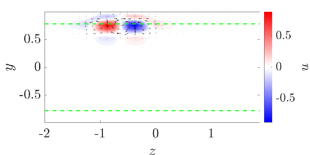
We next consider a case with the same parameters, but with a periodic domain in the spanwise direction, which we explicitly discretize rather than taking a Fourier transform. The numerical domain $[-h,h]\times[-2h,2h]$ is discretized using 32 Chebyshev and Fourier modes in the wall-normal and spanwise directions, respectively. Fig. 2 shows representative leading resolvent forcing and response from applying both standard and sparse resolvent analysis. Standard resolvent analysis gives modes that span the entire spanwise extent, consisting of alternating streaks of fast- and slow-moving fluid in the streamwise direction, located near the critical layers. These correlate with wall-normal velocity towards and away from the wall, respectively, indicative the presence of a lift-up amplification mechanism [45, 46]. The wall-normal and spanwise velocity components form streamwise vortices located between streamwise velocity streaks, as is typical of the near-wall cycle. Sparse resolvent analysis gives a mode with similar characteristics, though localized in one region of the domain, with a single dominant pair of fast- and slow-moving regions, which each have a smaller spanwise extent. This indicates that sparse resolvent analysis can be applied to identify spatially-localized structures in directions of spatial homogeneity. These sparse forcing and response modes can be interpreted as "minimal unit" structures corresponding to similar amplification as the spanwise-periodic structures identified from standard resolvent analysis. In this case, the amplification of the leading sparse modes is approximately 95% of that of the leading standard resolvent modes. While not shown, here suboptimal sparse modes consist of translations of this structure along each of the critical layers.

In this section, for laminar channel (Poiseuille) flow, we first perform (standard) resolvent analysis of the space-time resolvent operator (defined in Eq. (18)) and show results consistent with those from standard space-only resolvent analysis (defined in Eq. (12)).

We next applying the sparsity-promoting variant on the space-time resolvent operator to find structures that are localized in both space and time. Here and throughout, time is implicitly nondimensionalized by the maximum streamwise flow speed, $U_{0}$, and channel half-height, $h$. The numerical domain $[-h,h]\times[0,\tau)$ is discretized using 101 and 201 collocation points in the wall-normal and time dimensions, respectively.

Fig. 3 shows the wall-normal velocity ($v$) and vorticity ($\eta$) components of the leading resolvent forcing and response modes for laminar channel flow, with temporal domain $t\in[0,\tau)$ with $\tau=100$, for a representative set of parameters $k_{x}h=2$, $k_{z}h=1$, and outer Reynolds number $Re=hU_{0}/\nu=1500$. Unlike standard space-only resolvent analysis, we emphasize that here we do not specify a temporal frequency, but rather identify resolvent modes that are functions of both space and time. Here we identify modes that have constant amplitude in time but oscillating phase, consistent with Fourier modes. The modes shown have vorticity response components localized near the critical layer (determined by the inferred temporal frequency and streamwise wavenumber). The forcing and response modes tilt in opposite directions, consistent with amplification through the Orr mechanism [47, 48] (note that the direction of inclination is opposite to what would be observed if the horizontal axis was $x$ rather than $t$, as is shown in Fig. 4(a)). The wall-normal velocity response mode components consist of upright structures extending across the full height of the domain. Regions with $v$ directed away from the wall corresponds to regions of low $\eta$ and vice-versa, consistent with the lift-up mechanism transporting momentum in the $y$-direction.

These modes should be identical to those identified using standard resolvent analysis across all permissible frequencies (i.e. $\omega=k2\pi/\tau$ with $k\in\mathbb{Z}$). To confirm this, in Fig. 4(b) we compare the leading singular values of the temporally-localized resolvent operator with the maximal singular values obtained from traditional resolvent analysis over a range of permissible frequencies. The agreement between the singular values supports the premise that, for a stationary base/mean flow, space-time resolvent analysis indeed compiles the results of performing standard resolvent analysis across a range of permissible frequencies.

We now consider sparse space-time resolvent analysis for the same configuration and parameters. Fig. 5 depicts the sparse leading resolvent mode that were obtained for $\gamma=0.01$, allowing direct comparison with the non-sparse resolvent modes presented in Fig. 3. These response modes look similar to those shown for standard (non-sparse) space-time resolvent analysis, except for being localized both in time and space. The vorticity components of the forcing and response modes are again concentrated in a localized region near the critical layer corresponding to the frequency of oscillation of the phase of the modes, while the wall-normal velocity components extend over a wider region of the domain. The forcing modes show a slightly greater degree of spatial localization than the response modes, particularly for the vorticity component. Note that the forcing and response modes shown in Fig. 5 are computed using Eqs. (25)-(26), rather than being the direct output of the sparse optimization method. For comparison, we additionally show the raw output of optimizing Eq. (23) in Fig. 5. Only the vorticity component is shown, since for this choice of sparsity parameter $\gamma$, the wall-normal velocity component is zero. Comparison between Figs. 5 and 6 shows how applying Eqs. (25)-(26) modifies the raw sparse response modes to give structures more closely resembling the leading standard resolvent modes, at the expense of sparsity. In particular, in this case applying Eqs. (25)-(26) gives a response mode that spans over a less localized region, as well as nonzero wall-normal velocity components. Note that for both standard and sparse resolvent analysis, the wall-normal vorticity has a much larger response for these parameters.

The behavior of the time-localized modes is further studied by considering the strucutre of the modes at certain instances of time. In Fig. 7, we visualize the leading sparse response mode in vorticity along the streamwise axis at three different locations in time. These show how the mode amplitude grows and then decays over time, while the streamwise inclination of the modes increases. The time-localization of these structures can be observed more directly in Fig. 8, which depicts the cross-sections along the $t$-axis of the first three sparse response modes in vorticity at the spatial locations of largest mode amplitude. These cross sections show that the identified localized temporal functions appear to resemble Gaussian envelopes, with approximately constant phase gradient. This could provide evidence for a natural wavelet template for performing time-localized resolvent analysis with a prescribed wavelet basis. The structure of these temporal modes also suggests a connection with similar wavepacket templates that have been shown to closely approximate spatial resolvent modes [21, 49].

We now consider a system where the mean velocity profile varies in time. In particular, we consider a Stokes boundary layer configuration, where we again have flow between two parallel plates, but without an imposed pressure gradient, and where the boundaries move with a velocity

$$U_{w}(t)=U_{{0}}\cos(\Omega t)$$

(28)

We consider a Reynolds number based on the Stokes boundary layer thickness $\delta_{\Omega}=\sqrt{2\nu/\Omega}$ of $Re_{\Omega}=U_{0}\delta_{\Omega}/\nu=1500$. At this Reynolds number, the flow is intermittently turbulent [50, 51, 52, 53]. The time-periodic mean velocity profile for this configuration is shown in Fig. 9.

In this section, we again first consider space-time resolvent analysis with the standard optimization problem, before considering the sparsity-promoting variant on the observed time-resolved structures, allowing for the identification of time-localized structures corresponding to large linear amplification. Here and throughout, time is implicitly nondimensionalized by the characteristic velocity, $U_{0}$, and channel half-height, $h$. The numerical domain $[-h,h]\times[0,\tau)$ is discretized using 121 and 201 collocation points in the wall-normal and time dimensions, respectively.

Fig. 10 shows the wall-normal velocity and vorticity components of the leading resolvent forcing and response modes for a turbulent Stokes boundary layer, over a time domain that spans over three boundary layer cycles. Throughout this section we consider streamwise and spanwise wavenumbers $k_{x}h=k_{z}h=3\pi$. Although this system is time-periodic, the fact that it is not statistically-stationary means that each space-time resolvent mode does not necessarily correspond to a single Fourier mode in time. Indeed, the amplitude of the leading modes depicted in Fig. 10(a)-(d) is not exactly constant in time. Comparison between the real components of the velocity and vorticity of the response modes (Fig. 10(e)-(h)) indicates that wall-normal velocity directed away from (towards) the wall corresponds to positive (negative) values of wall-normal vorticity, in turn indicative of positive (negative) streamwise velocity fluctuations, suggesting the presence of the lift-up mechanism transporting momentum away from the side-walls.

The real components of this forcing and response mode oscillate with a period equal to the mean. To study the relationship between the mean and leading resolvent modes more directly, we show in Fig. 11(a)-(b) a comparison between the $\eta$-component of the leading resolvent forcing and response mode with the mean velocity profile. We observe a phase shift of approximately a quarter of a period between the mean and resolvent mode contours, for both the forcing and response. In contrast, for these parameters there is little phase shift between the forcing and response mode components, as shown in Fig. 11(c).

Lastly, in order to further investigate the time-evolving structures identified by this analysis, we present the corresponding physical mode as a function of $x$ and $y$ (by undoing the Fourier transform in the streamwise direction) of the leading space-time response mode in vorticity along with the instantaneous turbulent mean at three time instances in Fig. 12. The observed periodicity of the space-time modes manifests as the changing phase of the physical modes in the vicinity of the side-walls, following the temporal evolution of the turbulent mean. Interestingly, the inclination of the modes shown in Fig. 12(a)-(c) is in the opposite direction to that which would be expected for a stationary mean profile, where the response modes tilt in the same direction as the mean profile (e.g. as consistent with the Orr mechanism).

We now consider sparse space-time resolvent analysis of the same configuration. Fig. 13 shows the leading sparse forcing and response resolvent mode components obtained for a sparsity parameter $\gamma=0.01$ (in analogy to Fig. 10 for the non-sparse case). In order to best highlight the sparsity of the observed structures, in this case the time domain spans six periods of the mean flow. The sparse resolvent method identifies oscillating structures that are localized both in space and time, though for these parameters the mode components each span several oscillation periods. We observe as expected that the forcing mode components tend to precede the corresponding response mode components. In addition, the wall-normal velocity components precede the wall-normal vorticity, again indicating an energy transfer pathway consistent with the lift-up mechanism.

Fig. 14(a-b) shows the relationship between the $\eta$-component of the forcing and response modes with the mean velocity. Again (c.f. Fig. 11) we observe a quarter-period shift between the resolvent modes and mean. Fig. 14(c) confirms that the $\eta$-component of the forcing and response modes are again in-phase for these parameters. These findings suggest that the sparsity-promoting method is identifying a time-localized version of the same mechanism that was identified using the standard optimization method.

The temporal evolution of the sparse response mode shown in Fig. 15 also shows similar behavior to that observed for the non-sparse modes, with a mode inclination angle in the $x-y$ plane that appears to tilt in the opposite direction to the mean velocity profile at a given instant in time.

Lastly, the temporal evolution of the sparse response modes at the locations of maximum amplitude $y_{0}$ are shown in Fig. 16. In contrast to the statistically-stationary mean case considered in Fig. 8, here we observe more complex temporal envelopes, which cannot necessarily be closely approximated by a single simple prescribed template function.

References

- Schmid and Henningson [2001] Schmid, P., and Henningson, D. S., Stability and Transition in Shear Flows, Springer, New York, NY, 2001.
- McKeon and Sharma [2010] McKeon, B. J., and Sharma, A. S., “A critical-layer framework for turbulent pipe flow,” Journal of Fluid Mechanics, Vol. 658, 2010, pp. 336–382.
- Holmes et al. [2012] Holmes, P., Lumley, J. L., Berkooz, G., and Rowley, C. W., Turbulence, coherent structures, dynamical systems and symmetry, Cambridge University Press, 2012.
- Lumley [1967] Lumley, J. L., “The structure of inhomogeneous turbulent flows,” Proceedings of the International Colloquium on the Fine Scale Structure of the Atmosphere and its Influence on Radio Wave Propagation, edited by A. M. Yaglam and V. I. Tatarsky, Doklady Akademii Nauk SSSR, Moscow, Nauka, 1967.
- Towne et al. [2018] Towne, A., Schmidt, O. T., and Colonius, T., “Spectral proper orthogonal decomposition and its relationship to dynamic mode decomposition and resolvent analysis,” Journal of Fluid Mechanics, Vol. 847, 2018, pp. 821–867.
- Ren et al. [2021] Ren, J., Mao, X., and Fu, S., “Image-based flow decomposition using empirical wavelet transform,” Journal of Fluid Mechanics, Vol. 906, 2021, p. A22.
- Floryan and Graham [2021] Floryan, D., and Graham, M. D., “Discovering multiscale and self-similar structure with data-driven wavelets,” Proceedings of the National Academy of Sciences, Vol. 118, No. 1, 2021, p. e2021299118.
- Schmidt and Schmid [2019] Schmidt, O. T., and Schmid, P. J., “A conditional space–time POD formalism for intermittent and rare events: example of acoustic bursts in turbulent jets,” Journal of Fluid Mechanics, Vol. 867, 2019.
- Frame and Towne [2022] Frame, P., and Towne, A., “Space-time POD and the Hankel matrix,” arXiv preprint arXiv:2206.08995, 2022.
- Henningson et al. [1993] Henningson, D. S., Lundbladh, A., and Johansson, A. V., “A mechanism for bypass transition from localized disturbances in wall-bounded shear flows,” Journal of Fluid Mechanics, Vol. 250, 1993, pp. 169–207.
- Candès and Wakin [2008] Candès, E. J., and Wakin, M. B., “An introduction to compressive sampling,” IEEE signal processing magazine, Vol. 25, No. 2, 2008, pp. 21–30.
- Brunton et al. [2016] Brunton, S. L., Proctor, J. L., and Kutz, J. N., “Discovering governing equations from data by sparse identification of nonlinear dynamical systems,” Proceedings of the National Academy of Sciences, Vol. 113, No. 15, 2016, pp. 3932–3937.
- Loiseau and Brunton [2018] Loiseau, J.-C., and Brunton, S. L., “Constrained sparse Galerkin regression,” Journal of Fluid Mechanics, Vol. 838, 2018, pp. 42–67.
- Rubini et al. [2020] Rubini, R., Lasagna, D., and Da Ronch, A., “The l1-based sparsification of energy interactions in unsteady lid-driven cavity flow,” Journal of Fluid Mechanics, Vol. 905, 2020.
- Jovanović et al. [2014] Jovanović, M. R., Schmid, P. J., and Nichols, J. W., “Sparsity-promoting dynamic mode decomposition,” Physics of Fluids (1994-present), Vol. 26, No. 2, 2014, 024103.
- Tu et al. [2014] Tu, J. H., Rowley, C. W., Kutz, J. N., and Shang, J. K., “Spectral analysis of fluid flows using sub-Nyquist-rate PIV data,” Experiments in Fluids, Vol. 55, No. 9, 2014, pp. 1–13.
- Skene et al. [2022] Skene, C., Yeh, C.-A., Schmid, P., and Taira, K., “Sparsifying the Resolvent Forcing Mode via Gradient-Based Optimisation,” Journal of Fluid Mechanics, Vol. 944, 2022.
- Sharma and McKeon [2013] Sharma, A. S., and McKeon, B. J., “On coherent structure in wall turbulence,” Journal of Fluid Mechanics, Vol. 728, 2013, pp. 196–238.
- Luhar et al. [2015] Luhar, M., Sharma, A. S., and McKeon, B. J., “A framework for studying the effect of compliant surfaces on wall turbulence,” Journal of Fluid Mechanics, Vol. 768, 2015, pp. 415–441.
- McKeon [2017] McKeon, B. J., “The engine behind (wall) turbulence: perspectives on scale interactions,” Journal of Fluid Mechanics, Vol. 817, 2017, p. P1.
- Dawson and McKeon [2019] Dawson, S. T. M., and McKeon, B. J., “On the shape of resolvent modes in wall-bounded turbulence,” Journal of Fluid Mechanics, Vol. 877, 2019, pp. 682–716.
- Lesshafft et al. [2019] Lesshafft, L., Semeraro, O., Jaunet, V., Cavalieri, A. V. G., and Jordan, P., “Resolvent-based modeling of coherent wave packets in a turbulent jet,” Physical Review Fluids, Vol. 4, No. 6, 2019, p. 063901.
- Abreu et al. [2020] Abreu, L. I., Cavalieri, A. V., Schlatter, P., Vinuesa, R., and Henningson, D. S., “Spectral proper orthogonal decomposition and resolvent analysis of near-wall coherent structures in turbulent pipe flows,” Journal of Fluid Mechanics, Vol. 900, 2020.
- Towne et al. [2020] Towne, A., Lozano-Durán, A., and Yang, X., “Resolvent-based estimation of space–time flow statistics,” Journal of Fluid Mechanics, Vol. 883, 2020.
- Pickering et al. [2021] Pickering, E., Towne, A., Jordan, P., and Colonius, T., “Resolvent-based modeling of turbulent jet noise,” The Journal of the Acoustical Society of America, Vol. 150, No. 4, 2021, pp. 2421–2433.
- Yeh et al. [2020] Yeh, C.-A., Benton, S. I., Taira, K., and Garmann, D. J., “Resolvent analysis of an airfoil laminar separation bubble at Re= 500 000,” Physical Review Fluids, Vol. 5, No. 8, 2020, p. 083906.
- Bae et al. [2020] Bae, H. J., Dawson, S. T. M., and McKeon, B. J., “Resolvent-based study of compressibility effects on supersonic turbulent boundary layers,” Journal of Fluid Mechanics, Vol. 883, 2020, p. A29.
- Padovan et al. [2020] Padovan, A., Otto, S., and Rowley, C., “Analysis of amplification mechanisms and cross-frequency interactions in nonlinear flows via the harmonic resolvent,” Journal of Fluid Mechanics, Vol. 900, 2020.
- Padovan and Rowley [2022] Padovan, A., and Rowley, C. W., “Analysis of the dynamics of subharmonic flow structures via the harmonic resolvent: Application to vortex pairing in an axisymmetric jet,” Physical Review Fluids, Vol. 7, No. 7, 2022, p. 073903.
- Hein and Bühler [2010] Hein, M., and Bühler, T., “An inverse power method for nonlinear eigenproblems with applications in 1-spectral clustering and sparse PCA,” Advances in Neural Information Processing Systems, Vol. 23, 2010.
- Jolliffe et al. [2003] Jolliffe, I. T., Trendafilov, N. T., and Uddin, M., “A modified principal component technique based on the LASSO,” Journal of computational and Graphical Statistics, Vol. 12, No. 3, 2003, pp. 531–547.
- Zou et al. [2006] Zou, H., Hastie, T., and Tibshirani, R., “Sparse principal component analysis,” Journal of computational and graphical statistics, Vol. 15, No. 2, 2006, pp. 265–286.
- Sigg and Buhmann [2008] Sigg, C. D., and Buhmann, J. M., “Expectation-maximization for sparse and non-negative PCA,” Proceedings of the 25th international conference on Machine learning, 2008, pp. 960–967.
- Journée et al. [2010] Journée, M., Nesterov, Y., Richtárik, P., and Sepulchre, R., “Generalized power method for sparse principal component analysis.” Journal of Machine Learning Research, Vol. 11, No. 2, 2010.
- Zou and Xue [2018] Zou, H., and Xue, L., “A selective overview of sparse principal component analysis,” Proceedings of the IEEE, Vol. 106, No. 8, 2018, pp. 1311–1320.
- Bühler [2014] Bühler, T., “A flexible framework for solving constrained ratio problems in machine learning,” Ph.D. thesis, Saarland University, 2014.
- Bae et al. [2018] Bae, H. J., Lozano-Duran, A., Bose, S., and Moin, P., “Turbulence intensities in large-eddy simulation of wall-bounded flows,” Physical Review Fluids, Vol. 3, No. 1, 2018, p. 014610.
- Bae et al. [2019] Bae, H. J., Lozano-Durán, A., Bose, S. T., and Moin, P., “Dynamic slip wall model for large-eddy simulation,” Journal of fluid mechanics, Vol. 859, 2019, pp. 400–432.
- Lozano-Durán and Bae [2019] Lozano-Durán, A., and Bae, H. J., “Characteristic scales of Townsend’s wall-attached eddies,” Journal of fluid mechanics, Vol. 868, 2019, pp. 698–725.
- Orlandi [2000] Orlandi, P., Fluid flow phenomena: a numerical toolkit, Vol. 55, Springer Science & Business Media, 2000.
- Kim and Moin [1985] Kim, J., and Moin, P., “Application of a fractional-step method to incompressible Navier-Stokes equations,” Journal of computational physics, Vol. 59, No. 2, 1985, pp. 308–323.
- Wray [1990] Wray, A. A., “Minimal storage time advancement schemes for spectral methods,” NASA Ames Research Center, California, Report No. MS, Vol. 202, 1990.
- Weideman and Reddy [2000] Weideman, J. A., and Reddy, S. C., “A MATLAB differentiation matrix suite,” ACM Transactions on Mathematical Software (TOMS), Vol. 26, No. 4, 2000, pp. 465–519.
- Jiménez and Pinelli [1999] Jiménez, J., and Pinelli, A., “The autonomous cycle of near-wall turbulence,” Journal of Fluid Mechanics, Vol. 389, 1999, pp. 335–359.
- Landahl [1975] Landahl, M. T., “Wave breakdown and turbulence,” SIAM Journal on Applied Mathematics, Vol. 28, No. 4, 1975, pp. 735–756.
- Landahl [1980] Landahl, M. T., “A note on an algebraic instability of inviscid parallel shear flows,” Journal of Fluid Mechanics, Vol. 98, No. 2, 1980, pp. 243–251.
- Orr [1907] Orr, W. M., “The stability or instability of the steady motions of a perfect liquid and of a viscous liquid. Part II: A viscous liquid,” Proceedings of the Royal Irish Academy. Section A: Mathematical and Physical Sciences, JSTOR, 1907, pp. 69–138.
- Jiménez [2013] Jiménez, J., “How linear is wall-bounded turbulence?” Physics of Fluids, Vol. 25, No. 11, 2013, p. 110814.
- Dawson and McKeon [2020] Dawson, S. T. M., and McKeon, B. J., “Prediction of resolvent mode shapes in supersonic turbulent boundary layers,” International Journal of Heat and Fluid Flow, Vol. 85, 2020, p. 108677.
- Akhavan et al. [1991] Akhavan, R., Kamm, R., and Shapiro, A., “An investigation of transition to turbulence in bounded oscillatory Stokes flows Part 1. Experiments,” Journal of Fluid Mechanics, Vol. 225, 1991, pp. 395–422.
- Verzicco and Vittori [1996] Verzicco, R., and Vittori, G., “Direct simulation of transition in Stokes boundary layers,” Physics of Fluids, Vol. 8, No. 6, 1996, pp. 1341–1343.
- Vittori and Verzicco [1998] Vittori, G., and Verzicco, R., “Direct simulation of transition in an oscillatory boundary layer,” Journal of Fluid Mechanics, Vol. 371, 1998, pp. 207–232.
- Costamagna et al. [2003] Costamagna, P., Vittori, G., and Blondeaux, P., “Coherent structures in oscillatory boundary layers,” Journal of Fluid Mechanics, Vol. 474, 2003, pp. 1–33.