Wavelet-based resolvent analysis for statistically-stationary and temporally-evolving flows

The incompressible Navier-Stokes equations in Einstein notation are given by

$$\frac{\partial\bar{u}_{i}}{\partial{t}}+\bar{u}_{j}\frac{\partial\bar{u}_{i}}{\partial{x_{j}}}=-\frac{1}{\rho}\frac{\partial\bar{p}}{\partial x_{i}}+\nu\frac{\partial^{2}\bar{u}_{i}}{\partial{x}_{j}\partial{x}_{j}},\quad\frac{\partial\bar{u}_{i}}{\partial{x_{i}}}=0,$$

(1)

where $\bar{u}_{i}$ is the total velocity (including the mean and the fluctuating component), $\tilde{p}$ is the total pressure, $\rho$ is the density, and $\nu$ is the kinematic viscosity. The total velocity can be divided into $\bar{u}_{i}=U_{i}+u_{i}$, where $U_{i}$ is the average over ensembles and homogeneous directions, and $u_{i}$ is the fluctuating component. Similarly, pressure can be decomposed as $\tilde{p}=P+p$.

Equation (1) can then be divided into the mean and the fluctuating equations

	$$\displaystyle\frac{\partial{U_{i}}}{\partial t}+\left\langle\bar{u}_{j}\frac{\partial\bar{u}_{i}}{\partial{x_{j}}}\right\rangle=-\frac{1}{\rho}\frac{\partial{P}}{\partial{x_{i}}}+\nu\frac{\partial^{2}U_{i}}{\partial{x_{j}}\partial{x_{j}}},\quad\frac{\partial{U_{i}}}{\partial{x_{i}}}=0,$$		(2)
	$$\displaystyle\frac{\partial{u_{i}}}{\partial t}+U_{j}\frac{\partial{u_{i}}}{\partial{x_{j}}}+u_{j}\frac{\partial{U_{i}}}{\partial{x_{j}}}=-\frac{1}{\rho}\frac{\partial{p}}{\partial{x_{i}}}+\nu\frac{\partial^{2}u_{i}}{\partial{x_{j}}\partial{x_{j}}}+f_{i},\quad\frac{\partial{u_{i}}}{\partial{x_{i}}}=0,$$		(3)

where $f_{i}$ is the remaining nonlinear terms in the fluctuating equations and $\langle\cdot\rangle$ is the average over ensembles and in homogeneous directions. Note that some of the terms in the fluctuating equations may be zero depending on the flow configuration. The equations above do not have an analytic solution unless in very particular situations and are most commonly solved numerically. Discretizing the fluctuating equations, we get

$$D_{t}{u_{i}}+U_{j}D_{j}{u_{i}}+u_{j}dU_{i,j}=-\frac{1}{\rho}D_{i}{p}+\nu L{u_{i}}+f_{i},\quad D_{i}u_{i}=0,$$

(4)

where $D_{t}$ is the discrete derivative in time, $D_{i}$ is the discrete derivative in the $x_{i}$ direction, $L$ is the discrete Laplacian, and $dU_{i,j}$ denotes the matrix form of $\partial U_{i}/\partial x_{j}$. Each discretized equation is an $N_{t}\times N_{x_{1}}\times N_{x_{2}}\times N_{x_{3}}$-dimensional system, where $N_{t}$ is the temporal resolution, and $N_{x_{i}}$ are the spatial resolutions in the $x_{i}$, $i=1,2,3$ directions respectively. The discretized velocity and velocity gradient, $U_{j}$ and $dU_{i,j}$, are $(N_{t}\times N_{x_{1}}\times N_{x_{2}}\times N_{x_{3}})^{2}$ diagonal matrices. In the traditional resolvent analysis, we apply the Fourier transform operator in homogeneous directions and time, $F$, to the left in Eq. (4), leading to the equation

$$(FD_{t}F^{-1})(F{u_{i}})+(FU_{j}D_{j}F^{-1})(F{u_{i}})+(Fu_{j})(FdU_{i,j}F^{-1})=\\ -\frac{1}{\rho}(FD_{i}F^{-1})(F{p})+\nu(FLF^{-1})(F{u_{i}})+Ff_{i},\quad(FD_{i}F^{-1})(Fu_{i})=0,$$

(5)

where $F^{-1}$ is the inverse transformation, or equivalently

$$\widehat{D_{t}}\hat{u}_{i}+\widehat{U_{j}D_{j}}\hat{u}_{i}+\widehat{dU_{i,j}}\hat{u}_{j}=-\frac{1}{\rho}\widehat{D_{i}}\hat{p}+\nu\hat{L}\hat{u}_{i}+\hat{f}_{i},\quad\widehat{D_{i}}\hat{u}_{i}=0.$$

(6)

Note that for an arbitrary matrix $M$ and vector $b$, $\hat{M}:=FMF^{-1}$ and $\hat{b}:=Fb$. For temporally stationary systems, this equation can typically be decoupled for each wavenumber and frequency combination. For example, in the case of channel flow where the flow is homogeneous in the streamwise ($x_{1}$) and spanwise ($x_{3}$) directions, the linear operator can be cast as

$$\left[\begin{array}[]{c}\hat{u}_{1}(k_{1},k_{3},\omega)\\ \hat{u}_{2}(k_{1},k_{3},\omega)\\ \hat{u}_{3}(k_{1},k_{3},\omega)\\ \hat{p}(k_{1},k_{3},\omega)\end{array}\right]=\hat{\mathcal{H}}(k_{1},k_{3},\omega)\left[\begin{array}[]{c}\hat{f}_{1}(k_{1},k_{3},\omega)\\ \hat{f}_{2}(k_{1},k_{3},\omega)\\ \hat{f}_{3}(k_{1},k_{3},\omega)\\ 0\end{array}\right]$$

(7)

for a given $(k_{1},k_{3},\omega)$ triplet. Typically, the singular value decomposition of the linear operator $\hat{\mathcal{H}}\in\mathbb{C}^{4N_{x_{2}}}\times\mathbb{C}^{4N_{x_{2}}}$ is taken to study the left and right singular vectors as response and forcing modes, and the singular values as amplification factors or gains.

We first compare the results of both the traditional Fourier-based resolvent analysis and wavelet-based resolvent analysis. For this, we consider a turbulent channel flow. The mean profile of a turbulent channel flow at friction Reynolds number $Re_{\tau}=186$ is obtained by a direct numerical simulation (DNS) using a second-order staggered finite-difference [35] and a fractional-step method [36] with a third-order Runge-Kutta time-advancing scheme [37]. Periodic boundary conditions are imposed in the streamwise and spanwise directions and the no-slip and no-penetration boundary conditions are used at the top and bottom walls. The code has been validated in previous studies in turbulent channel flows [38, 39, 40] and flat-plate boundary layers [41]. The numerical domain is $8\pi\delta\times 2\delta\times 3\pi\delta$ and is discretized using 768, 130, and 288 grid points in the streamwise, wall-normal, and spanwise directions, respectively. We use uniform grid spacing in the streamwise and spanwise directions of $\Delta x_{1}^{+}=6$ and $\Delta x_{3}^{+}=6$, and a wall-normal grid stretched away from the wall using a hyperbolic tangent with $\min(\Delta x_{2}^{+})=0.16$ and $\max(\Delta x_{2}^{+})=7.2$. Here the superscript $+$ denotes wall units defined in terms of $\nu$ and $u_{\tau}$, where $u_{\tau}$ is the friction velocity. The simulations were run for 100 eddy turnover times (defined as $\delta/u_{\tau}$) after transients to compute the mean quantities.

For the resolvent analysis, the wall-normal direction is discretized using a Chebyshev collocation method using $N_{x_{2}}=128$, and the mean streamwise velocity profile and its wall-normal derivative from the DNS are interpolated to the Chebyshev collocation points. We use a periodic boundary condition for the temporal domain, $T$, with a temporal resolution of $N_{t}=128$. We choose $D_{t}$ to be a Fourier differentiation matrix, and $D_{x_{2}}$ a Chebyshev differentiation matrix with a no-slip and no-penetration boundary condition at the wall. Note that these matrices are not sparse; for this case, sparse differentiation matrices were not needed, though finite difference matrices may be used in higher-dimensional problems to improve efficiency. We choose the spanwise and streamwise wavelengths of $\lambda_{1}^{+}\approx 1000$ and $\lambda_{3}^{+}\approx 100$, in line with the most energetic structures close to the wall.

Since the mean profiles are statistically steady, we have $\widetilde{U_{j}D_{j}}=\widehat{U_{j}D_{j}}$, $\widetilde{dU_{i,j}}=\widehat{dU_{i,j}}$, $\tilde{L}=\hat{L}$. The wavelet- and Fourier-based cases thus only differ by the time differentiation matrix such that $W^{-1}\widetilde{D_{t}}W=F^{-1}\hat{D}_{t}F=D_{t}$. Note that $W$ is unitary for the choice of wavelet. Since the singular value decomposition is unique up to multiplication by a unitary matrix, we expect the singular values of $\tilde{\mathcal{H}}$ to be the same as that of

$$\hat{\mathcal{H}}(k_{1},k_{3})=\left(\begin{array}[]{cccc}\hat{\mathcal{H}}(k_{1},k_{3},\omega_{1})&&&\\ &\hat{\mathcal{H}}(k_{1},k_{3},\omega_{2})&&\\ &&\hat{\mathcal{H}}(k_{1},k_{3},\omega_{3})&\\ &&&\ddots\\ \end{array}\right),$$

(16)

where $\omega_{i}=(2\pi i)/T$ for $i=-{N_{t}}/{2},\cdots,{N_{t}}/{2}-1$. Here, we set $T=5.5\delta/u_{\tau}$. Moreover, we expect the response and forcing modes of both systems to be related by the unitary transform given by the Fourier and inverse-wavelet transform in time, $FW^{-1}$. In Fig. 2(a), we show the singular values of the leading Fourier- and wavelet-based resolvent response modes, $\hat{\psi}$ and $\tilde{\psi}$ respectively. The Fourier-based resolvent modes were computed by applying the resolvent analysis at each $\omega_{i}$ and taking the principal singular value. The wavelet-based resolvent modes were computed by solving the full space-time system at once. We also plot the most amplified streamwise resolvent response mode for the two methods in Fig. 2(b). As expected, the singular values and the corresponding modes are equivalent. The small deviations in the singular values for the two cases are due to the truncation errors of the Shannon wavelet basis.

The added advantage of the wavelet-based method lies in its ability to preserve temporal localization, which lets us formulate a time-scale sensitive resolvent for transient flows even when the mean profiles are statistically stationary. For this, we use the windowed wavelet-based resolvent analysis framework from §3.2.2, but setting the windowing of the response modes, $\mathcal{C}$, to the identity matrix. We then calculate the resolvent modes of $\tilde{\mathcal{H}}\mathcal{B}$. The principal forcing mode will lie in the span of a subset of the complete wavelet basis, as selected by $\mathcal{B}$. By picking a particular wavelet scale and shift via $\mathcal{B}$, we can restrict the forcing to a chosen frequency range, mostly localized in a particular time range.

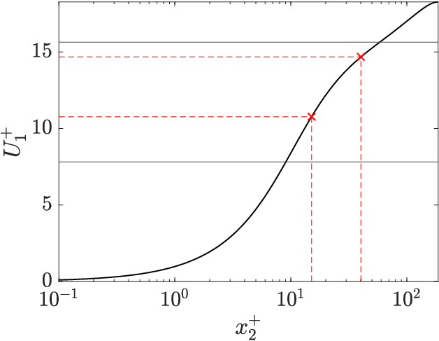
To demonstrate this capability, we study the effect of a time-localized forcing on the buffer layer ($x_{2}^{+}\in[15,40]$). We choose $\mathcal{B}$ such that the forcing modes are limited to a single wavelet with the frequency range containing the critical layer corresponding to the buffer layer, i.e., $[U(x_{2}^{+}=15),U(x_{2}^{+}=40)]=[\omega_{\min},\omega_{\max}]/k_{1}$ (Fig. 3). For the current case, we have $\omega_{\min}=12.52{u_{\tau}}/{\delta}$ and $\omega_{\max}=17.17{u_{\tau}}/{\delta}$. We pick a temporal resolution of $N_{t}=64$, and a time horizon of $T=5.5{\delta}/{u_{\tau}}$. We project the flow variables onto Shannon wavelets that cover frequency intervals $(2^{-i-1}{N_{t}}/{T})([-2\pi,-\pi]\cup[\pi,2\pi])$, for $i=0,1,\cdots 5$. The windowing matrix $\mathcal{B}$ is chosen to restrict the forcing to the unshifted wavelet ($\tau=0$, i.e., centered at $t=0$) that has been scaled to cover $[9.14,18.28]{u_{\tau}}/{\delta}$ (i.e. $i=1$).

The resulting principal response mode is confined to the frequency band determined by the forcing, as shown in Fig. 4(a), which is expected since the time scales are decoupled for statistically stationary flows. The response mode additionally varies in time; the magnitude of the mode growth as a function of time is shown in Fig. 4(b). The principal response mode peaks at a time $tu_{\tau}/\delta=0.79$ before decaying. This transient growth can be explained by the non-normality of the linearized system [42]. The response modes at three different time shifts are shown in Fig. 5. The modes are predominantly in the streamwise direction, forming alternating low- and high-speed streamwise streaks. Although not shown, the principal forcing mode only has a small contribution from the streamwise direction and is in the form of streamwise rolls, in line with the linear theory [43, 44, 45] and the self-sustaining process of wall turbulence [46, 47, 48, 49, 50, 51, 10].

The Stokes boundary layer is simulated through a channel flow with the lower and upper walls oscillating in tandem at a velocity of $U_{w}(t)=U_{\max}$ cos$(\Omega t)$ with no imposed pressure gradient. The relevant nondimensional number is the Reynolds number $Re_{\Omega}=U_{\max}\delta_{\Omega}/\nu$, where $\delta_{\Omega}=\sqrt{2\nu/\Omega}$ denotes the Stokes boundary layer thickness. For the current case, we consider $Re_{\Omega}=1500$, which lies within the intermittently turbulent regime [52, 53, 54, 55, 56]. This problem has been well-studied numerically and experimentally in the literature [52, 57, 58, 53, 54, 55, 56, 59, 60, 61, 62, 63]. The same numerical solver used to simulate the turbulent channel flow is used to generate the statistics, with modifications in the boundary condition to accommodate the oscillating walls. The domain size of the channel for the DNS is given by $6\pi\delta_{\Omega}\times 80\delta_{\Omega}\times 3\pi\delta_{\Omega}$ and discretized using $64$, $385$ and $64$ points in each direction. We compute the mean velocity profiles by averaging in homogeneous directions and phase. Fig. 6 shows the mean and the root-mean-square (rms). velocity profiles at three different temporal locations. Note that $U_{1}(t\Omega+\pi)=-U(t\Omega)$ and $U_{i,rms}(t\Omega+\pi)=U_{i,rms}(t\Omega)$. We observe that the turbulent energy peaks near the wall at $t\Omega=2.65$ and propagates away from the wall in time.

To construct the resolvent operator, we first choose the spatial scales for the homogeneous directions. Using the DNS data, we calculate the streamwise energy spectrum at $x_{2}/\delta_{\Omega}=1.43$ and $t\Omega=2.51$, which correspond to the peak spatio-temporal location of the $U_{1,rms}$. The most energetic streamwise and spanwise scales at that location are given by $k_{1}\delta_{\Omega}=0.67$ and $k_{3}\delta_{\Omega}=2.67$, which we choose as the streamwise and spanwise scales for the resolvent operator. We use $N_{x_{2}}=140$ and $N_{t}=780$ to solve the discrete system. We construct $D_{t}$ and $D_{x_{2}}$ as sparse finite difference matrices. We additionally choose the time-derivative operator $D_{t}$ to be circulant to enforce periodicity in time. We compute the modes for the half-channel and modify $D_{x_{2}}$ to enforce a no-slip and no-penetration boundary condition at the wall, and a free-slip and no-penetration boundary condition at the centerline.

The principal input and output modes corresponding to the chosen spatial scales and boundary conditions in time are shown in Fig. 7(a). We observe that the principal input and output modes are synchronized with the peaks in $U_{1,rms}$. The energy propagation towards the center occurs at a similar rate for the resolvent modes as for the DNS results. This suggests that the energy amplification in the Stokes boundary layer can partially be explained by the optimal linear mechanism, as for turbulent channel flow [45]. Moreover, we observe that the principal input modes precede the principal output modes with time delay, and thus a transient growth mechanism can be explained through the wavelet-based resolvent modes. This is in line with a physical interpretation of the modes in which the input modes ‘cause’ the output modes. In Fig. 7(b), we show the magnitude of the response modes in the frequency-time plane, which highlights that the bulk of the response is limited to a single wavelet scale and a few time shifts. Using the windowed resolvent operator to restrict our forcing and our response to the first wavelet scale, we indeed obtain nearly identical modes as in 7 while reducing the effective dimension of our resolvent operator by a factor of four.

Fig. 8 shows that the peak amplification occurs at the location of zero mean streamwise velocity. This is in line with the fact that Fourier-based resolvent modes are often centered around a critical layer [2], where the critical layer $x_{2}=x_{2}^{c}$ is defined as $U_{1}(x_{2}^{c})=c$ and $k_{x}c=\omega$. For the Stokes boundary layer with the chosen length scales, the critical layer seems to occur at $U_{1}(x_{2}^{c})=0$, which corresponds to $\omega=0$. For this time-periodic problem, we note that wavelet resolvent analysis should be equivalent to a harmonic resolvent analysis [13] that includes the interactions between all the resolved time scales. The wavelet resolvent modes should indeed map to the harmonic resolvent modes via an inverse wavelet transform and a Fourier transform in time. We expect that harmonic resolvent analysis will also reveal a peak amplification for waves at $\omega=0$; we will conduct a harmonic resolvent analysis on this system and compare it with the wavelet-based resolvent modes in future works.

Finally, we study a fully-developed turbulent channel flow at $Re_{\tau}=186$ that is subjected to a sudden lateral pressure gradient $dP/dx_{3}=\Pi dP/dx_{1}$ at $t=0$ with $\Pi=30$ [65, 64]. This flow, commonly referred to as a three-dimensional (3D) channel flow, has an initial transient period dominated by 3D non-equilibrium effects. Eventually, the flow will reach a new statistically steady state with the mean flow in the $(dP/dx_{1},dP/dx_{3})$ direction parallel to the wall. In the transient period, the tangential Reynolds stress initially decreases before increasing linearly, with depletion and increase rate that scales as $\Pi x_{2}/\delta$ [64].

The mean flow profiles are obtained from [64] and have nonzero streamwise and spanwise components $U_{1}$ and $U_{3}$ (Fig. 9) as well as nonzero wall-normal gradients of streamwise and spanwise components $dU_{1,2}$ and $dU_{3,2}$. The time domain of the simulation is $Tu_{\tau,0}/\delta=2.34$, where $u_{\tau,0}$ is the initial friction velocity. To construct the discrete resolvent operator, we use a spatial resolution of $N_{x_{2}}=65$ for the half-channel, and a finite difference matrix $D_{x_{2}}$ enforcing a no-slip and no-penetration boundary condition at the wall and a free-slip and no-penetration condition at the centerline. The boundary condition for the temporal finite difference operator $D_{t}$ is chosen to enforce a Neumann-type condition, $\partial_{t}(\cdot)|_{t=0}=\partial_{t}(\cdot)|_{t=T}=0$. To reduce the impact of the boundary condition on the modes at $t=0$ we extend $U_{1}$ and $U_{3}$ to the time interval $tu_{\tau,0}/\delta\in[-0.58,2.34]$ and assume $U_{i}(t\leq 0,y)=U_{i}(t=0,y)$ and $dP/dx_{3}(t<0)=0$. When the modes are plotted, we only show the original time domain $tu_{\tau,0}/\delta\in[0,2.34]$ and exclude the contribution from negative times. We use a temporal resolution of $N_{t}=1000$ for the extended time frame.

Regarding the spatial scales for the homogeneous directions, we choose $(\lambda_{1}^{+},\,\lambda_{3}^{+})=(1000,\,100)$ as well as ($\lambda_{1}^{+},\,\lambda_{3}^{+})=(189,\,1890)$ and $(\lambda_{1}^{+},\,\lambda_{3}^{+})=(297,\,2970)$. Here, $(\cdot)^{+}$ indicates the wall scaling with respect to $u_{\tau,0}$, before the lateral pressure gradient is applied. The first combination of $\lambda_{1}^{+}$ and $\lambda_{3}^{+}$ is the same as in §4.1 and corresponds to the spatial scales preferred by the near-wall streaks at $Re_{\tau}=186$ prior to the lateral pressure gradient. The resolvent modes for these scales are shown in Fig. 11(a,b). The magnitude of the modes in frequency-time space is also plotted in Fig. 12(a). The resolvent modes are temporally centered around $t=0$ and exhibit a predominant streamwise component. The modes are located in a region $x_{2}/\delta<0.25$, which corresponds to $x_{2}^{+}<45$, i.e., the buffer region. Thus, at $t=0$, the modes capture the highly energetic near-wall streaks. The subsequent temporal decay of these modes can be explained by the changing flow conditions, notably the growth of the spanwise wall-shear stress $\tau_{3}$, and consequently $u_{\tau}$ (see Figure 10). Under these conditions, the spatial scales preferred by the near-wall streaks stretch as $u_{\tau}$ increases and the wall-shear stress tensor rotates toward the $x_{3}$ direction.

The second and third pairs of spatial scales are chosen so that the resolvent modes can capture the near-wall streaks under the new shear condition at times $t\Omega=1.3$ and $t\Omega=1.94$ respectively. To take into account the stronger mean shear in the spanwise direction, which increases proportionally to $dP/dx_{3}$ [64], the quantities in wall units must be scaled by a factor of $u_{\tau}(t)/u_{\tau,0}$. We also take into account the new orientation of the streaks by applying a rotation by the wall-shear stress angle $\gamma(t)=\tan^{-1}(\tau_{3}/\tau_{1})$, where $\tau_{i}$ is the instantaneous wall-shear stress in the $x_{i}$ direction (see Fig. 10). The new spatial scales are calculated by rotating a box of size $\lambda_{1}^{+}=100(u_{\tau}(t)/u_{\tau,0})$ and $\lambda_{3}^{+}=1000(u_{\tau}(t)/u_{\tau,0})$ with angle $\gamma(t)$ and finding the length scales aligned with the $x_{1}$ and $x_{3}$ axis. The response mode for the second pair of spatial scales, $\lambda_{1}^{+}=189$ and $\lambda_{3}^{+}=1890$, correspond to $t\Omega=1.3$ and are plotted in 11(c,d). The frequency-time map of the modes is shown in Fig. 12(b). Similar to the first case, the modes are centered around $t\Omega=1.3$, indicating that the wavelet-based resolvent analysis is able to identify the nonequilibrium effects of the non-stationary flow. We note that the spanwise component of the response mode is much more dominant than the streamwise component, which reflects the new wall-shear angle $\gamma=75.7^{\circ}$. We also observe that the modes are closer to the wall, which depict the reduction of the buffer layer as a result of the increase in $u_{\tau}$. Finally, for the third case, we choose $\lambda_{1}^{+}=297$ and $\lambda_{3}^{+}=2970$. We observe that these modes (Fig. 11e,f and Fig. 12c) are not centered around $t\Omega=1.94$. We speculate that this is due to the temporal boundary condition at $t\Omega=2.34$. As the flow is not at a statistically-steady state at this time, a Neumann boundary condition may not be the most suitable boundary condition. The modes cannot grow beyond the boundary due to the boundary condition and are artificially damped near the end of the temporal domain.

References

- Jovanović and Bamieh [2005] Jovanović, M. R., and Bamieh, B., “Componentwise energy amplification in channel flows,” J. Fluid Mech., Vol. 534, 2005, pp. 145–183.
- McKeon and Sharma [2010] McKeon, B. J., and Sharma, A. S., “A critical-layer framework for turbulent pipe flow,” J. Fluid Mech., Vol. 658, 2010, pp. 336–382.
- Sharma and McKeon [2013] Sharma, A. S., and McKeon, B. J., “On coherent structure in wall turbulence,” J. Fluid Mech., Vol. 728, 2013, pp. 196–238.
- Moarref et al. [2013] Moarref, R., Sharma, A. S., McKeon, B. J., and Tropp, J. A., “Model-based scaling and prediction of the streamwise energy intensity in high-Reynolds number turbulent channels,” J. Fluid Mech., Vol. 734, 2013, pp. 275–316.
- Luhar et al. [2014] Luhar, M., Sharma, A. S., and McKeon, B. J., “Opposition control within the resolvent analysis framework,” J. Fluid Mech., Vol. 749, 2014, pp. 597–626.
- Martini et al. [2020] Martini, E., Cavalieri, A. V. G., Jordan, P., Towne, A., and Lesshafft, L., “Resolvent-based optimal estimation of transitional and turbulent flows,” J. Fluid Mech., Vol. 900, 2020, p. A2.
- Towne et al. [2020] Towne, A., Lozano-Durán, A., and Yang, X. I. A., “Resolvent-based estimation of space–time flow statistics,” J. Fluid Mech., Vol. 883, 2020, p. A17.
- Bae et al. [2021] Bae, H. J., Lozano-Durán, A., and McKeon, B. J., “Nonlinear mechanism of the self-sustaining process in the buffer and logarithmic layer of wall-bounded flows,” J. Fluid Mech., Vol. 914, 2021, p. A3.
- Yeh and Taira [2019] Yeh, C.-A., and Taira, K., “Resolvent-analysis-based design of airfoil separation control,” J. Fluid Mech., Vol. 867, 2019, pp. 572–610.
- Bae et al. [2020a] Bae, H. J., Dawson, S. T. M., and McKeon, B. J., “Resolvent-based study of compressibility effects on supersonic turbulent boundary layers,” J. Fluid Mech., Vol. 883, 2020a, p. A29.
- Bae et al. [2020b] Bae, H. J., Dawson, S. T. M., and McKeon, B. J., “Studying the effect of wall cooling in supersonic boundary layer flow using resolvent analysis,” AIAA Scitech 2020 Forum, 2020b, p. 0575.
- Ahmed et al. [2021] Ahmed, M. A., Bae, H. J., Thompson, A. F., and McKeon, B. J., “Resolvent analysis of stratification effects on wall-bounded shear flows,” Phys. Rev. Fluids, Vol. 6, 2021, p. 084804.
- Padovan et al. [2020] Padovan, A., Otto, S. E., and Rowley, C. W., “Analysis of amplification mechanisms and cross-frequency interactions in nonlinear flows via the harmonic resolvent,” J. Fluid Mech., Vol. 900, 2020, p. A14.
- Meyer [1992] Meyer, Y., Wavelets and Operators: Volume 1, Cambridge University Press, 1992.
- Meneveau [1991] Meneveau, C., “Analysis of turbulence in the orthonormal wavelet representation,” J. Fluid Mech., Vol. 232, 1991, pp. 469–520.
- Lewalle [1993] Lewalle, J., “Wavelet transforms of the Navier-Stokes equations and the generalized dimensions of turbulence,” Appl. Sci. Res., Vol. 51, No. 1-2, 1993, pp. 109–113.
- Ren et al. [2021] Ren, J., Mao, X., and Fu, S., “Image-based flow decomposition using empirical wavelet transform,” J. Fluid Mech., Vol. 906, 2021, p. A22.
- Floryan and Graham [2021] Floryan, D., and Graham, M. D., “Discovering multiscale and self-similar structure with data-driven wavelets,” Proc. Natl. Acad. Sci. USA, Vol. 118, No. 1, 2021, p. e2021299118.
- Towne et al. [2018] Towne, A., Schmidt, O. T., and Colonius, T., “Spectral proper orthogonal decomposition and its relationship to dynamic mode decomposition and resolvent analysis,” J. Fluid Mech., Vol. 847, 2018, pp. 821–867.
- Abreu et al. [2020] Abreu, L. I., Cavalieri, A. V. G., Schlatter, P., Vinuesa, R., and Henningson, D. S., “Spectral proper orthogonal decomposition and resolvent analysis of near-wall coherent structures in turbulent pipe flows,” J. Fluid Mech., Vol. 900, 2020, p. A11.
- Tissot et al. [2021] Tissot, G., Cavalieri, A. V. G., and Mémin, E., “Stochastic linear modes in a turbulent channel flow,” J. Fluid Mech., Vol. 912, 2021, p. A51.
- Jeun et al. [2016] Jeun, J., Nichols, J. W., and Jovanović, M. R., “Input-output analysis of high-speed axisymmetric isothermal jet noise,” Phys. Fluids, Vol. 28.4, 2016, p. 047101.
- Kojima et al. [2020] Kojima, Y., Yeh, C., Taira, K., and Kameda, M., “Resolvent analysis on the origin of two-dimensional transonic buffet,” J. Fluid Mech., Vol. 885, 2020, p. R1.
- Mallat [2001] Mallat, S., A Wavelet Tour of Signal Processing, Academic Press, 2001.
- Najmi [2012] Najmi, A.-H., Wavelets: A Concise Guide, The Johns Hopkins University Press, 2012.
- Alappat et al. [2020] Alappat, C., Basermann, A., Bishop, A. R., Fehske, H., Hager, G., Schenk, O., Thies, J., and Wellein, G., “A recursive algebraic coloring technique for hardware-efficient symmetric sparse matrix-vector multiplication,” ACM Trans. Parallel Comput., Vol. 7, No. 3, 2020, pp. 1–37.
- Bollhöfer et al. [2020] Bollhöfer, M., Schenk, O., Janalik, R., Hamm, S., and Gullapalli, K., “State-of-the-art sparse direct solvers,” Parallel Algorithms in Computational Science and Engineering, Springer, 2020, pp. 3–33.
- Bollhöfer et al. [2019] Bollhöfer, M., A., E., Scheidegger, S., and Schenk, O., “Large-Scale Sparse Inverse Covariance Matrix Estimation,” SIAM J. Sci. Comput., Vol. 41, No. 1, 2019, pp. A380–A401.
- Simon and Zha [2000] Simon, H. D., and Zha, H., “Low-rank matrix approximation using the Lanczos bidiagonalization process with applications,” SIAM Journal on Scientific Computing, Vol. 21, No. 6, 2000, pp. 2257–2274.
- Halko et al. [2011] Halko, N., Martinsson, P.-G., and Tropp, J. A., “Finding structure with randomness: Probabilistic algorithms for constructing approximate matrix decompositions,” SIAM review, Vol. 53, No. 2, 2011, pp. 217–288.
- Drineas and Mahoney [2016] Drineas, P., and Mahoney, M. W., “RandNLA: randomized numerical linear algebra,” Communications of the ACM, Vol. 59, No. 6, 2016, pp. 80–90.
- Tropp et al. [2017] Tropp, J. A., Yurtsever, A., Udell, M., and Cevher, V., “Practical sketching algorithms for low-rank matrix approximation,” SIAM Journal on Matrix Analysis and Applications, Vol. 38, No. 4, 2017, pp. 1454–1485.
- Ribeiro et al. [2020] Ribeiro, J. H. M., Yeh, C.-A., and Taira, K., “Randomized resolvent analysis,” Phys. Rev. Fluids, Vol. 5, No. 3, 2020, p. 033902.
- Yeh et al. [2020] Yeh, C.-A., Benton, S. I., Taira, K., and Garmann, D. J., “Resolvent analysis of an airfoil laminar separation bubble at Re= 500 000,” Physical Review Fluids, Vol. 5, No. 8, 2020, p. 083906.
- Orlandi [2000] Orlandi, P., Fluid Flow Phenomena: A Numerical Toolkit, Fluid Flow Phenomena: A Numerical Toolkit, Springer, 2000.
- Kim and Moin [1985] Kim, J., and Moin, P., “Application of a fractional-step method to incompressible Navier-Stokes equations,” J. Comp. Phys., Vol. 59, 1985, pp. 308–323.
- Wray [1990] Wray, A. A., “Minimal-storage time advancement schemes for spectral methods,” Tech. rep., NASA Ames Research Center, 1990.
- Bae et al. [2018] Bae, H. J., Lozano-Durán, A., Bose, S. T., and Moin, P., “Turbulence intensities in large-eddy simulation of wall-bounded flows,” Phys. Rev. Fluids, Vol. 3, 2018, p. 014610.
- Bae et al. [2019] Bae, H. J., Lozano-Durán, A., Bose, S. T., and Moin, P., “Dynamic slip wall model for large-eddy simulation,” J. Fluid Mech., Vol. 859, 2019, pp. 400–432.
- Lozano-Durán and Bae [2019] Lozano-Durán, A., and Bae, H. J., “Characteristic scales of Townsend’s wall-attached eddies.” J. Fluid Mech., Vol. 868, 2019, p. 698.
- Lozano-Durán et al. [2018] Lozano-Durán, A., Hack, M. J. P., and Moin, P., “Modeling boundary-layer transition in direct and large-eddy simulations using parabolized stability equations,” Phys. Rev. Fluids, Vol. 3, 2018, p. 023901.
- Schmid and Henningson [2000] Schmid, P. J., and Henningson, D. S., Stability and Transition in Shear Flows, Vol. 142, Springer Science & Business Media, 2000.
- Orr [1907] Orr, W., “The stability or instability of the steady motions of a perfect liquid and of a viscous liquid. Part I: A perfect liquid,” Proc. R. Ir. Acad., Vol. A 27, 1907, pp. 9–68.
- Landahl [1975] Landahl, M. T., “Wave breakdown and turbulence,” SIAM J. Appl. Math, Vol. 28, No. 4, 1975, pp. 735–756.
- Jiménez [2013] Jiménez, J., “How linear is wall-bounded turbulence?” J. Fluid Mech., Vol. 25, 2013, p. 110814.
- Jiménez and Moin [1991] Jiménez, J., and Moin, P., “The minimal flow unit in near-wall turbulence,” J. Fluid Mech., Vol. 225, 1991, pp. 213–240.
- Hamilton et al. [1995] Hamilton, J. M., Kim, J., and Waleffe, F., “Regeneration mechanisms of near-wall turbulence structures,” J. Fluid Mech., Vol. 287, 1995, pp. 317–348.
- Jiménez and Pinelli [1999] Jiménez, J., and Pinelli, A., “The autonomous cycle of near-wall turbulence,” J. Fluid Mech., Vol. 389, 1999, pp. 335–359.
- Waleffe [1997] Waleffe, F., “On a self-sustaining process in shear flows,” Phys. Fluids, Vol. 9, No. 4, 1997, pp. 883–900.
- Schoppa and Hussain [2002] Schoppa, W., and Hussain, F., “Coherent structure generation in near-wall turbulence,” J. Fluid Mech., Vol. 453, 2002, pp. 57–108.
- Farrell et al. [2017] Farrell, B. F., Gayme, D. F., and Ioannou, P. J., “A statistical state dynamics approach to wall turbulence,” Phil. Trans. R. Soc. Lond. A, Vol. 375, No. 2089, 2017, p. 20160081.
- Hino et al. [1976] Hino, M., Sawamoto, M., and Takasu, S., “Experiments on transition to turbulence in an oscillatory pipe flow,” J. Fluid Mech., Vol. 75, No. 2, 1976, pp. 193–207.
- Akhavan et al. [1991] Akhavan, R., Kamm, R. D., and Shapiro, A. H., “An investigation of transition to turbulence in bounded oscillatory Stokes flows Part 1. Experiments,” J. Fluid Mech., Vol. 225, 1991, pp. 395–422.
- Verzicco and Vittori [1996] Verzicco, R., and Vittori, G., “Direct simulation of transition in Stokes boundary layers,” Phys. Fluids, Vol. 8, No. 6, 1996, pp. 1341–1343.
- Vittori and Verzicco [1998] Vittori, G., and Verzicco, R., “Direct simulation of transition in an oscillatory boundary layer,” J. Fluid Mech., Vol. 371, 1998, pp. 207–232.
- Costamagna et al. [2003] Costamagna, P., Vittori, G., and Blondeaux, P., “Coherent structures in oscillatory boundary layers,” J. Fluid Mech., Vol. 474, 2003, pp. 1–33.
- Spalart and Baldwin [1989] Spalart, P. R., and Baldwin, B. S., “Direct simulation of a turbulent oscillating boundary layer,” Turbulent shear flows 6, Springer, 1989, pp. 417–440.
- Jensen et al. [1989] Jensen, B. L., Sumer, B. M., and Fredsøe, J., “Turbulent oscillatory boundary layers at high Reynolds numbers,” J. Fluid Mech., Vol. 206, 1989, pp. 265–297.
- Von Kerczek and Davis [1974] Von Kerczek, C., and Davis, S. H., “Linear stability theory of oscillatory Stokes layers,” Journal of Fluid Mechanics, Vol. 62, No. 4, 1974, pp. 753–773.
- Sarpkaya [1993] Sarpkaya, T., “Coherent structures in oscillatory boundary layers,” Journal of Fluid Mechanics, Vol. 253, 1993, pp. 105–140.
- Blondeaux and Vittori [1994] Blondeaux, P., and Vittori, G., “Wall imperfections as a triggering mechanism for Stokes-layer transition,” Journal of Fluid Mechanics, Vol. 264, 1994, pp. 107–135.
- Carstensen et al. [2010] Carstensen, S., Sumer, B. M., and Fredsøe, J., “Coherent structures in wave boundary layers. Part 1. Oscillatory motion,” Journal of Fluid Mechanics, Vol. 646, 2010, pp. 169–206.
- Ozdemir et al. [2014] Ozdemir, C. E., Hsu, T.-J., and Balachandar, S., “Direct numerical simulations of transition and turbulence in smooth-walled Stokes boundary layer,” Physics of Fluids, Vol. 26, No. 4, 2014, p. 045108.
- Lozano-Durán et al. [2021] Lozano-Durán, A., Giometto, M. G., Park, G. I., and Moin, P., “Non-equlibrium three-dimensional boundary layers at moderate Reynolds numbers,” J. Fluid Mech., Vol. 883, 2021, p. A20.
- Moin et al. [1990] Moin, P., Shih, T.-H., Driver, D. M., and Mansour, N. N., “Direct numerical simulation of a three-dimensional turbulent boundary layer,” Phys. Fluids, Vol. 2, No. 10, 1990, pp. 1846–1853.