Constructing Operator Basis in Supersymmetry: A Hilbert Series Approach
Abstract
In this paper we introduce a Hilbert series approach to build the operator basis for a supersymmetry theory with chiral superfields. We give explicitly the form of the corrections that remove redundancies due to the equations of motion and integration by parts. In addition, we derive the maps between the correction spaces. This technique allows us to calculate the number of independent operators involving chiral and antichiral superfields to arbitrarily high mass dimension. Using this method, we give several illustrative examples.
1 Introduction
Effective field theory (EFT) is a framework which allows one to extend the Standard Model (SM) to include new physics effects. In EFT, higher dimensional operators encode our ignorance and also extends the theory up to a certain scale. There are many ways to form higher dimension operators by adding fields and derivatives but not all of these operators are independent. For example, within the Standard Model effective field theory it is difficult to determine the minimal operator basis above dimension six due to several redundancies in operator space Grzadkowski:2010es. However, in the past few years, Hilbert series techniques have provided an illuminating framework within which one is able to quickly count the number of independent operators at certain dimensions Lehman:2015via; Henning:2015daa; Lehman:2015coa; Henning:2017fpj; Anisha:2019nzx; Marinissen:2020jmb; Graf:2020yxt; Wang:2021wdq; Graf:2022rco; Yu2022; Yu2022a; Yu2021; Lu2021; Lu2022; Sun2022. Several other methods, such as the on-shell Young Tableau construction Henning:2019enq; Henning:2019mcv; Ma:2019gtx; Durieux:2019siw; Dong:2021yak; Li:2022tec; Fonseca:2019yya; Li:2020gnx, also serve as complementary ways to give the number and explicit form of these operators. Using these tools, a complete list of independent dimension seven through nine operators can now be found in the literature Henning:2015alf; Murphy:2020rsh; Kobach:2017xkw; Gunawardana:2017zix; Liao:2020jmn; Li2021.
Supersymmetry, as the largest spacetime symmetry compatible with an interacting theory, is still a possible candidate for physics BSM. Higher derivative operators in supersymmetry have been studied in several articles Antoniadis:2007xc; Forcella:2008tqe; Farakos:2013zsa; Dudas:2015vka; Nitta:2020gam especially within the context of supersymmetry breaking. Therefore determining the operator basis in supersymmetry may be important, specially in order to avoid including operators that are related. However, there are difficulties that arise when applying the above mentioned EFT counting methods to a supersymmetric theory. The usual Hilbert series approach only works for Lorentz invariant as well as gauge invariant operator spaces. Once we include supersymmetry, it cannot directly give the correct counting, because the definition of integration by parts changes due to the additional fermionic derivatives in supersymmetric theories.
In this paper we develop a method that allows one to build the operator basis of all dimensions in a supersymmetric theory with only chiral/antichiral superfields 11 1 The inclusion of vector superfields will be postponed to a forthcoming publication.. Hilbert series and related group theory techniques are fundamental to tackle the problem in hand, and together with the definition of correction spaces (vector spaces of redundancies), provide a systematic way to remove all dependencies and get an operator basis. Using a recursive derivation, we are able to derive all corrections explicitly.
This paper is organized as follows. In Section 2 we introduce the Hilbert series approach and how to apply it to form Lorentz invariants. Then we review supersymmetry in the language of superspace, and use Hilbert series tools to build the operator space we are interested in. Section 3 deals with the two kinds of redundancies, namely EOM and IBP relations. Specifically, in Section 3.1 we show how to remove EOM. The method to remove IBP relations in non-supersymmetric theory is introduced in Section 3.2, leading to the definition of correction space, which allows one to identify corrections in a systematic way. We then generalize this idea and derive explicit corrections at each order in Section 3.3, where three examples that involve chiral superfields and antichiral superfields are given at the end. Finally, in Section 4 we give a brief summary and some possible future applications of this approach. Proofs and character formulae are given in the appendices22 2 Through out the paper we adopt the most-negative metric tensor in Minkowski space, i.e. . Totally antisymmetric tensor in two dimensions are defined to be . In addition, a useful identity we will use is ..
2 Hilbert series and supersymmetry reviewed
2.1 Hilbert series and plethystic exponential
The Hilbert series Pouliot:1998yv; Benvenuti:2006qr; Butti:2007jv; Feng:2007ur; Forcella:2007wk; Dolan:2007rq; Gray:2008yu; Hanany:2008sb; Benvenuti:2010pq; Chen:2011wn; Hanany:2012dm; Rodriguez-Gomez:2013dpa; Dey:2013fea; Hanany:2014hia; Hanany:2014dia is a useful way to count the number of independent group invariants. In a field theory consisting of fields, the Hilbert series has the following form:
| (1) |
where is the number of independent invariants composed of powers of and derivatives. Technically, the above are complex numbers to label the content of fields, i.e. spurions, and similarly is a complex number to label the partial derivative. To count the number of independent operators now becomes the same as calculating .
One technique to calculate the Hilbert series is via the plethystic exponential (PE) Butti:2007jv; Gray:2008yu; Hanany:2008sb; Benvenuti:2010pq; Hanany:2014dia. The plethystic exponential generates all (symmetric or anti-symmetric) products of its arguments. For our purposes, the arguments are spurions representing each field in the theory, multiplied by the character appropriate for that field’s representation under the spacetime (Lorentz) and internal symmetries defining the theory. For a field transforming under the representation of a simple group , the plethystic exponential is defined as:
| (2) |
where we assign for bosons (symmetric products) and for fermions (antisymmetric products). The characters can be expressed in terms of unimodular complex variables, where is the rank of . For example, is rank , so all characters can be written in terms of a single complex variable . We will sometimes list the complex variables that make up the characters as arguments in the PE, e.g. and refer to them as ‘group parameters’. Some explicit examples for and characters are given in Appendix A. A useful property of plethystic exponentials is:
| (3) |
which allows us to combine multiple fields into a single PE.
Expanded, the PE is a sum over all polynomials of its arguments (fields, for us), with each term in the polynomial multiplied by some combination of characters. To project out the polynomials that are net gauge/Lorentz invariants, we use character orthonormality:
| (4) |
where is the Haar measure of the group . The Haar measure can be treated as the group volume/measure defined on the group , and we give explictly its expression for common Lie groups in Appendix A. The above relation holds provided is compact. Specifically, integrating the PE times – the character of the trivial representation – over the Haar measure projects out invariants and gives us the Hilbert series. For the example of fields in a theory defined by group we get:
| (5) |
If the theory has multiple symmetries, the argument of the PE is the product of the individual group characters, and the invariants are projected out by integrating over all Haar measures. When considering the symmetries of a theory, we include all gauge and internal global symmetries along with Lorentz symmetry. For the latter, we work with representations of rather than since the former is compact and therefore its characters are orthonormal33 3 We only care about counting the invariants and not about the dynamics.. Since we have included the Lorentz group to the mix, we can add derivatives of fields to the PE, generating invariants of , , etc. Naively, we can include fields with derivatives by adding them to the PE, meaning we treat e.g. as an independent field species and add them to the PE dressed with the appropriate characters. What this naive approach misses are redundancies among operators with derivaives from integration by parts and the equations of motion. These require special attention and will be addressed in detail shortly.
Forgetting about derivatives for the moment, let us calculate the (zero derivative) Hilbert series for and , two familiar left-handed fermions from the SM, as an example. Both transform as under , and under , , . The argument of the plethystic exponential is given by:
| (6) |
where is the group parameter for , is the group parameter for , is the group parameter for and are group parameters for . Notice that there is an additional factor of 3, which represents the 3 generations. Plugging into the plethystic exponential integrating over all Haar measures, we get Lehman:2015via; Henning:2015alf
| (7) |
where 44 4 We could include the Haar measure for into as well, with group parameter . However, as none of the fields in the PE transform under , the integral is trivial.. We can therefore easily read out the number of operators from the expansion, i.e. 57 operators built from and 4818 operators built from .
Having reviewed how to construct the (zero-derivative) Hilbert series for scalar and spinor fields using the plethystic approach, in the next section we will generalize this technique to supersymmetry, where the non-supersymmetric fields are replaced by superfields. Since our aim is to study the operator basis, we first need to know what kind of operators a supersymmetric Lagrangian can contain.
2.2 supersymmetry
In this section we introduce the basic knowledge of supersymmetry, restricting ourselves to (anti-)chiral superfields. To define such superfields, we need two superderivatives , given by55 5 The 4-dimensional sigma matrices are defined to be: (8) :
| (9a) | ||||
| (9b) | ||||
where and are two-dimensional Grassmann numbers, and is the usual partial derivative. From now on, we use and to represent the two derivatives, i.e. and They satisfy the following anticommutation relation:
| (10) |
The (anti)commutation relations
| (11) |
will also prove useful in later sections.
Chiral superfields and antichiral superfields are defined to satisfy the following constraints:
| (12) |
They can be expanded in terms of component fields:
| (13) | ||||
| (14) |
where and represent superspace coordinates, is a complex scalar field, a Weyl chiral fermion and an auxiliary field.
The supersymmetric action built from chiral and antichiral superfields is formed as Weinberg:2000cr:
| (15) |
where and are holomorphic functions (superpotential) of chiral and antichiral superfields respectively, and is a real scalar function of both and , called the Kähler potential. The subscripts represent -term ( term) and -term ( term) respectively. For example, the explicit renormalizable Lagrangian for a single chiral superfield is given by:
| (16) |
where the two functions are chosen to be and .
To build the Hilbert series for supersymmetry with (anti)chiral superfields, we first need to know their characters. Since a chiral superfield contains both bosons and fermions, we choose the lowest component fields to represent – and respectively, which transform as scalar fields under the Lorentz group66 6 Note that the full supermultiplet can be built by acting supercharges on the lowest component field , i.e. , where and are group generators (supercharges) related to supersymmetry.. If we were only interested in superfield invariants without superderivatives, Eq. (5) is sufficient. Operators with superderivatives are where all the complications arise and will be the main focus of the rest of this paper.
Fields with one derivative, , have a lowest component that is fermionic. They carry Lorentz group representations , respectively, and must be added to the fermionic portion of the PE, meaning they enter the sum in Eq. (2) with a minus sign. As in non-supersymmetric theories, we can add operators with more superderivatives to the PE, e.g. to generate even higher derivative operators. There are three differences with respect to the non-supersymmetric case in this aspect. First, certain terms are zero because of the chiral/antichiral nature of the , e.g. , and should not be added. Second, we have to keep track of the bosonic/fermionic nature of the higher derivative terms. This is straightforward, as all terms with an even number of superderivatives acting on are bosonic, while all terms with an odd number of superderivatives are fermionic. Finally, it may seem that we need to study higher derivative extensions of the superpotential and Kähler potential separately, as they have different holomorphy properties. However, as we will show, any -term (superpotential term) containing superderivatives can be transformed into a -term (Kähler term). Therefore, to build our operator basis for (anti)chiral superfields with superderivatives, we only need to find the set of independent -terms.
To prove the last statement, let , where are chiral superfields that satisfy the chiral constraints and are general superfields. Since identically, are chiral superfields. As a result, constructed in this way is chiral and we can choose its -term to be part of the Lagrangian,
| (17) |
There are two kinds of terms that exist in , one is and another is , where labels one field. By definition, doesn’t carry any derivatives and we can simply drop such terms. The other term, , is the same as since due to the chiral constraint. As a result,
| (18) |
where we drop total derivatives in -spacetime when we go from the second line to third line.
We are then left to count the number of operators with an arbitrary number of superderivatives that can form a real function, the most general Kähler potential. To form an invariant, we need to form a Lorentz scalar, and therefore the number of superderivatives should be even to get fully contracted. In addition, due to the intrinsic existence of an R-symmetry – a symmetry that transforms the ’s – we have to put another constraint. We claim that an operator is R-invariant if it carries the same number of ’s and ’s. This is easily proved by noticing that each reduces one degree of (correspond to -1 to the R-charge), while each reduces one degree of (correspond to +1 to the R-charge). If we assign the R-charge 0 to (anti)chiral superfields77 7 For multiple flavours, we should assign R-charges to chiral superfields of different flavours., the field carries R-charge -1 while the field carries R-charge 1. So the lowest dimensional R-invariant Lorentz scalar we can form out of is . To incorporate R-symmetry into the Hilbert series, we need an additional group as well as the related group parameter .
Calculating the corresponding Hilbert series is straightforward by putting superfields together with their characters into the plethystic exponential and then integrating over the Haar measure. For example, suppose we want to form the Hilbert series with fields , whose representations are given by respectively; the last number represents the R-charge. Then the Hilbert series is formed as:
| (19) |
where represent the group parameters of and . The Haar measure in this case is , and the integrand in the PE is given by
| (20) |
Plugging (20) into (19) will generate all possible invariants constructed from these superfields.
Once we include fields with superderivatives in the PE, as in the example above, the Hilbert series generated by Eq. (5) ((19) for the example just shown) is not the end of the story. Operators must be independent (represent different contributions to the action) in an operator basis, and we have not yet removed redundancies from the Hilbert series coming from IBP or EOM relations. The first redundancy comes from the fact that two operators differing by a total derivative gives the same action after integrating over the full space (assuming the boundary terms vanish). The second redundancy comes from field redefinition, after which the original operator can be replaced with another operator with fewer derivatives. We will discuss in detail how to eliminate these two relations in the next section.
3 Removing EOM and IBP
3.1 EOM relations
To remove EOM relations from the operator space, we first look at the equation of motion of a free chiral superfield , given by:
| (21) |
where is the mass of the superfield. One can verify this by expanding both sides in component forms and then compare the lowest components:
| (22) |
where and are the lowest component fields of and . As expected, this reduces to the Klein-Gordon equation for a free complex scalar field. The equation of motion relations allow one to “replace” , , etc. within higher dimensional operators via field redefinitions Georgi:1991ch. Extrapolating this logic to superfields, we can swap factors of for , etc. within superfield operators.
The next question is how to enforce this in forming the Hilbert series, i.e. automatically removing redundant operators by manipulating the plethystic exponential. We will proceed as in non-supersymmetric theories, following Ref. Lehman:2015coa.
Specifically, using a scalar field theory as an example, we add to the PE as separate terms. As the PE generates all possible polynomials of its arguments, this gets us polynomials of and so on. To account for the EOM, we simply exclude from the PE, as any operator containing can be transformed by field redefinition to an operator without the , and thus already included in the operator counting. By the same logic, we drop etc. from the PE. Omitting these terms, we are left with only the symmetric derivatives at each order88 8 Antisymmetric combinations of derivatives are either zero (in the case of ordinary derivatives), or a field strength (if is charged under a gauge symmetry and the derivatives are covariant derivatives). In either case, the terms don’t appear as the building blocks in PE., , etc., where indicates traceless and symmetric pieces. In terms of characters, the PE argument for a scalar is
| (23) |
Here, the characters refer to representations under and is the spurion for the derivative, which we need to keep track of operator mass dimension; are the group parameters related to and .
For fermions, the process is the same – we extend the PE to include derivatives, but omit and its higher derivative counterparts. For example, for a left handed fermion , the PE argument is
| (24) |
While we will not consider field strengths in this paper, one can account for their EOM in a similar fashion Lehman:2015via.
The infinite series of higher derivatives in Eq. (23), (24) can be summed. The results are, respectively, the characters for the scalar and fermion (here, type)99 9 Technically, and importantly for the approach in Ref. Henning:2015daa; Henning:2017fpj, the characters one gets by summing the infinite series of derivatives are short representations of the conformal group. conformal group representations Dolan:2008vc; Dolan:2005wy; Dolan:2002zh. We’ll denote the conformal representations as and , so that Eq. (23), (24) can be expressed concisely as
| (25) |
Taking and to be the group parameters for and , the conformal characters are explicitly given by
| (26) |
where
| (27) |
Notice that the conformal characters contain spurion along with the Lorentz group characters. The connection of the conformal group is not coincidental and has been used in Ref. Henning:2017fpj to analyze the Hilbert series for non-supersymmetric theories.
The non-supersymmetric approach to EOM redundancy can be imported almost as is to the (chiral field) supersymmetric case. The complications are that i.) in supersymmetry we always have bosonic and fermionic fields, and ii.) there are two types of derivative. Both are easy to accommodate. For the two derivative types, we use as the spurion for and for – the connection between and from Eq. (10) implies . For and , we add derivatives following Eq. (23), simply substituting for 1010 10 The order of the two spurions P,Q doesn’t matter since they are not real quantum operators.. Ignoring symmetry for the moment,
| (28) |
where it is understood that the arguments of for the supersymmetric case are and the group parameters and . For the fermionic fields , , we follow Eq. (24),
| (29) |
The extra factors of and in the last line of Eq. (29) account for the fact that the fermionic fields already contain one superderivative. As there are two types of derivative, it may not be obvious that only symmetric derivative combinations should be included in the fermionic PE. To see why, consider the example , which is the same as when we anticommute the first two superderivatives and remove the piece that contains . However, expanding in component form we get – exactly the Dirac equation.
Putting the pieces together for a single chiral superfield (and its hermitian conjugate) and reinstating the symmetry with , the full PE is
| (30) |
where is the group parameter. Replacing , the PE can be extended to more chiral superfields. To account for fields with different charges, the full PE is the product over the individual -charge sectors.
Integrating the PE over the Haar measure for the Lorentz group, , and any additional gauge/internal symmetry groups, the resulting Hilbert series includes derivatives and accounts for EOM redundancies. IBP redundancies are more subtle, and will be explored in detail in the next section.
Before moving on, it is worth noting that while the Hilbert series contains all invariants, we are often only interested in invariants for a specific mass dimension. To address this, we can weight each spurion in the PE (both fields and derivative spurions) by their canonical mass dimension, e.g. , etc. then expand the PE to the desired order before integrating over the Haar measure. This not only allows us to organize the invariants by mass dimension, but it simplifies the contour integration over the group parameters greatly as the only residues after expanding in are at the origin.
Finally, as most phenomenological applications of supersymmetry involve renormalizable operators only, it is worth spending a little more time on the meaning of higher dimensional superfield operators. Theories with higher dimensional superfield operators come about from integrating out fields fully supersymmetrically, and can be arrived at by performing the path integral over heavy degrees of freedom Affleck:1984xz; Intriligator:1995au; Brizi:2009nn. If all operators (including superderivatives) are maintained at a certain mass dimension in the expansion, the theory in terms of superfield is guaranteed to be supersymmetric (up to even higher dimensional effects). While convenient, superfields contain auxiliary fields, which seem confusing at first when present in higher dimensional operators. However, within the basis selected by the Hilbert series – where as many derivatives as possible are removed via EOM – the auxiliary fields do not become dynamical. As such, if one wants to convert between a higher dimensional superfield operators into its components, we can remove auxiliary fields (again, up to even higher dimensional effects) by the component form of the EOM, (if a mass term is allowed by the charges).
3.2 IBP relations in non-supersymmetric theories
With the EOM relations taken care of, in this section we will study the IBP redundancies. We begin by reviewing how IBP redundancies are handled in Hilbert series for non-supersymmetric field theories. As we will show, the structure of the IBP corrections in the non-supersymmetric case will guide us towards a generalization that works for supersymmetry.
For non-supersymmetric field theories, IBP redundancies can be accounted for by adding a factor to the Haar measure integrand, Eq. (5) Henning:2015alf,
| (31) |
where is the same function of the derivative spurions and Lorentz group parameters and that we saw in the conformal characters (Eq. (26)),
| (32) |
To understand the how incorporates IBP relations, let’s expand it. Grouped by powers of , is the sum of five terms:
| (33) |
Plugged into the Haar measure integral, character orthonormality will project out different terms for each power of . The first term, , is the same as what we had without the factor of – it is the number of invariant operators and therefore sits in the Lorentz representation. Going forward, we’ll refer to this set of operators as . The second term comes with a minus sign and accompanies the character for the Lorentz representation, therefore when we perform the Haar integral we’ll project out all operators that are invariant under any internal/gauge symmetries but are Lorentz four-vectors – the operator set . By same logic, the term projects out all Lorentz representations, etc.
What does this have to do with IBP? Imagine we are looking at a theory of a single real scalar and care about counting invariant operators of the form . IBP relations manifest here in the ways we can shuffle how the derivatives are sprinkled among the fields, with two operators being equivalent if they differ only by a total derivative. The operators projected out by the term in Eq. (34) have the form . If we apply one final derivative to any of the operators, we have to get zero since it’s a total derivative. At the same time, must yield combination of operators. So, for every operator, we find some linear combination of operators that equals zero; and for each linear combination, we can solve for one of the operators in terms of the others, meaning it is not independent. For a more general (non-supersymmetric) theory, we can express the IBP relation as
| (34) |
As each operator implies one relation among operators, the number of operators taking all relations into account is the dimension of minus the dimension of space, exactly whats accomplished by the and terms in Eq. (33).
The factor doesn’t stop at because the IBP relations defined by Eq. (34) are not always independent. To correct for this, higher order corrections need to be taken into consideration. For example, if an operator in can be expressed as , where the denotes antisymmetrization, then identically. By the logic above, this zero means each operator implies a linear dependent relation among the previous equations:
| (35) |
Iterating, we see that the last two terms, which represent operator spaces and correct the and terms respectively. The expansion terminates at because in four dimensions we cannot form a non-trivial operator with five or more totally antisymmetric indices. Therefore no space can correct , and the series ends1111 11 One can understand the termination of the series by realizing that any total derivative is itself a closed but not exact d-forms Henning:2015daa; Henning:2017fpj, where d is the dimension of spacetime. In 4 dimensions, one can at most has a 4-form, whose basis is given by , with a coefficient carrying antisymmetic indices among . .
Putting things together, the number of independent operators modulo IBP in the non-supersymmetric case is given by
| (36) |
The above understanding of the factor sheds light on how to find similar factors in more general cases to remove IBP relations. For this purpose, we first give a definition of what is a correction and then apply it in the non-supersymmetric case to reproduce the . Starting with a space , we define the zeroth order equivalence relations on as follows:
| (37) |
where are maps that take elements from to and the sum runs over all possible and the dimension of each . The upper index indicates that this is the zeroth-order correction. The IBP relation for a non-supersymmetric theory fits right into this general definition if we identify as the space , as the space , and is ,
| (38) |
For non-supersymmetric theories, there is only one class, or branch, of corrections, so there is no index on , however for more general setups there may be multiple .
Next, we identify the space , along with maps . We call the first order correction space if all elements in satisfy the following conditions:
| (39) |
From the definition, we see the superscript indicates the order of the correction (1, here), while the subscript respectively label which of the and spaces are connected with the map. For a non-supersymmetric theory, again there is only one space – the operator set – thus the only map, , has . Clearly, all operators in satisfy
| (40) |
Higher-order corrections are defined in a similar way. A space is called the nth-order correction to if there exist maps , such that:
| (41) |
and is denoted as This notation allows us to keep track of all corrections and maps, such that we can easily prove whether a given space (or spaces) and related maps satisfy the definition. In our non-supersymmetric example, it is easy to see that the spaces and maps satisfy the criteria.
We can use diagrams to keep track of the corrections and spaces. Starting from the left, we place the space . Next comes , with arrows pointing from to indicating the maps . The second column is , with arrows from to the representing the maps . Next comes with its affiliated maps, then , and so on. For non-supersymmetric theories, the diagram is shown below in Fig. 1. There is only one correction space at each order (one , one , etc.), so the correction diagram is a single line; the leftmost space is , and the diagram ends with .

Having defined the corrections, we are now able to calculate the number of independent operators:
| (42) |
where the represents the number of operators in space. The series of corrections may terminate at some fixed order, as in the non-supersymmetric case, or it may continue infinitely. To execute this counting within the Hilbert series, each of the need to be dressed up with the appropriate Lorentz group characters – so the right spaces are projected out by character orthonormality – and multiplied by spurions representing the maps . In non-supersymmetric theories, the map spurions are all just , and the character/spurion dressed version of Eq. (42) reproduces .
There is a subtlety that we should mention. For non-supersymmetric theories the Hilbert series can be written as Henning:2017fpj. The procedure described above – plethystic exponential, conformal characters, and factor – reproduces . The pieces is a correction stemming from the non-orthonormality of the characters for short representations of the conformal group under the Haar measure for the (maximal compact subgroup of the conformal group). For scalars, spinors and field strengths in four dimensions, only includes terms of dimension four or less. So, while it is needed for full operator basis, plays no role if our interest is counting higher dimensional operators. Our approach for supersymmetric theories may also generate contributions to , however, as in the non-supersymmetric scenario, will only include operators with mass dimension four. As such, we will ignore for the remainder of this work, focusing on the (mass dimension ) terms contained in .
Now we have everything we need to study the more complicated supersymmetric case. As we will see in the next section, there are two independent IBP relations in supersymmetry, e.g. two spaces , and the maps take on a more complicated form. The net result is a more interesting and subtle correction structure.
3.3 IBP relations in supersymmetry
In a () supersymmetric theory, there are three possibilities two Kähler terms can differ by a total derivative – the IBP relations,
| (43) |
However, only two of these are independent. Use the defining anti-commutation relations between the two superderivatives , we can rewrite the third relation as:
| (44) |
which is a linear combination of the first two equations. Therefore there are only two independent possibilities in supersymmetry and we choose the first two to be the IBP relations. The above also means we only need two of to build operators. Following our choice for IBP relations, we’ll keep and ; roughly speaking, the reader looking to spot factors of should look for combinations or (exactly which depends on whether the object acted on by the derivatives is chiral, antichiral, or neither).
When two Kähler terms differ by a total derivative, they will give the same action once integrated over the superspace. For example, in the first case,
| (45) |
where in the third line the integration goes from the full superspace to half superspace, and in the fourth line the second term vanishes because . The fact that and give the same action means that we only need to take into account of one of them when we form the Lagrangian.
From now on, we will use a slightly different notation to label different spaces. Let and represent the number of and in each operator space, we define the space to be the space spanned by the basis determined by the Hilbert Series, where , and are the number of superderivatives of respectively in , the operator space we are interested in; see Table 1 for details. The indicates the spinorial structure of elements in that space. For example, if we want to study the case , then , , , etc. This notation explicitly shows how many superderivatives a space carries, making it easier for us to arrange and order different spaces. At times, we will omit the indices in for brevity, though they can be reconstructed knowing and .
Equations (45) and (43) motivate the following IBP equivalence relation
| (46) |
which fits into the zeroth order correction master formula Eq. (37) if we define two correction spaces with corresponding maps .
Using (39) and (41), we can fill out the entire diagram of higher order corrections spaces and maps. The result is shown below in Fig 2. Arrows point from the correction space to the space they correct, i.e. from to . The zeroth order corrections lie in the second column, and , with maps and connecting them to , as expected from Eq. (46). The higher corrections are naturally divided into six ‘branches’, three of which are oriented in the same direction as the zeroth order map and three which are oriented along the map direction. For simplicity, we’ll refer to these two groups as the ‘’ and ‘’ directions. They are symmetric under the change . The expressions for the higher order maps, and , are more complicated and will be given shortly. In addition to the multiple branches, another difference between the supersymmetric and non-supersymmetric cases is that the branches in supersymmetric theories do not terminate.

Notice that the number of spaces increases with the correction order: there are two , four , five , etc. To check if these spaces and the maps that connect them satisfy our map criteria Eq. (39), we need to choose a labeling scheme. We choose for the zeroth order corrections, for the first order, and for second order1212 12 For a different labeling, the only change would be in the indices. While the space of corrections in infinite, we have only listed the explicit labeling scheme for the spaces needed to prove the relations in the text.. Each space has both an name, which tells us the derivative content of its operators, and an name, which orients the map with respect to the original space , distinguishes between equidistant maps, and most compactly expresses the IBP relations. Table 1 below shows both names of the spaces we are interested in, along with their Lorentz group representation and characters.
| Corrections | |||
|---|---|---|---|
| Representation | Character | ||
| 1 | |||
| 1 | |||
| 1 | |||
| 1 | |||
The higher order corrections are best understood moving along the diagonal branches, rather than thinking in columns. In the following sections we will study the three ‘ branches’ in detail.
3.3.1 First branch
The first branch we study is shown in Fig. 3, continues along the direction and contains the correction spaces . This branch, and its complex conjugate branch, are the most similar to the non-supersymmetric case. We will use that similarity to intuit the result, then prove that all maps and spaces satisfy the required criteria (Eq. (39)).
Recall the counting formula given in (36). There, each space carries totally antisymmetric indices, and as a result vanishes when acting on two (commuting) partial derivatives. In four dimensions, the maximal number of fully antisymmetric indices is four, and therefore the series terminates at . Let’s try the same trick in the supersymmetry case. As all superderivatives are fermionic, i.e. anti-commuting, acting two of them on an operator that carries totally symmetric indices will vanish identically, i.e. . Each vanishing combinations implies a relation among operators and is thus a correction, just as in the non-supersymmetric case. However, the spacetime dimension places no restriction on operators with symmetric (Lorentz) indices an operator can carry. Therefore, in the supersymmetry case, this type of correction does not terminate at a fixed derivative order. In parallel with (36), we expect the counting formula for supersymmetric theories coming from this branch is given by:
| (47) |
Now we will prove this formula using the definition and give one example of the existence of higher order corrections.
It is clear that we can get relations among operators from acting on each term in . However, just as in the non-supersymmetric case, these relations may not be independent. For example, acting on and gives the same relations, even though they come from different terms. The reason is because of the fact that identically. It’s not difficult to extend this to general . We claim that corrects , where represents fully symmetrization of the indices. Any element in transforms under and the proof is straightforward as follows:
| (48) |
The second equation vanishes because of the antisymmetric property of superderivatives.

3.3.2 Second branch
In this section, we will study the second branch, shown in Fig. 4. The second branch is a new feature in supersymmetry, arising from the fact that the theory has two superderivatives as well as one ordinary partial derivative. Although they are not independent, two of them survive after removing one of them using the defining anticommutation relation (10). To see how the second branch comes about, let’s look at two examples at low dimensions, and then we give the general result and proof for arbitrary dimensions.

Suppose we want to build the operator basis for . Then we know that we can get the following IBP relations from and :
| (49a) | ||||
| (49b) | ||||
| (49c) | ||||
where we have dropped all EOM terms, e.g. or when acting with the final derivative; it is also important to remember that are Grassmann objects with indices raised/lowered with . It’s clear that , so only two of the above three relations are independent. The reason for the connection is that and can all be obtained from an operator with even fewer derivatives, . Specifically, and both are generated by applying to , while is generated from . As the three ‘daughters’ , and share a single ‘mother’, the relations they imply ( through ) are interconnected.
Let us verify that these maps do indeed satisfy Eq. (39). This will better illustrate how to unpack Eq. (39), as well as provide some more physical insight into the relations. Referring to Table 1, , , and we have already identified the zeroth order correction maps , . What remains are the maps taking us from to and . In the notation, the maps take to and , so . From the discussion above, we see and , where is defined as:
| (50) |
For future reference we also introduce the definition of acting on to give :
| (51) |
For these corrections, Eq. (39) becomes:
| (52) |
where the sign flips in the second and third lines come from changing the order of raised/lowered indices with , etc. and the last equality comes from Eq. (11). Using , we can get some intuition for the physics of the second correction. Starting from an operator in , we can get to either by applying a partial derivative first and then or by applying first and then . However, the connection between , and tells us these operations commute and the corrections are not independent.
Tracing through the above steps in Fig. 4 in green, we see the two paths ( then or vice versa) form a closed loop. The correspondence of the loops in the diagram with the commutation relation will help us identify other second order corrections directly from Fig. 2.
As a second example, consider the correction from the space . This space corrects and , both of which correct . Additionally also corrects . Using the notation introduced after Eq. (41), we can express this compound correction structure as . The maps required are (connecting ), (connecting to ), (connecting ), (connecting to ) and (connecting ). From our previous example, we know , and . If we make the identification , , the maps satisfy for all :
| (53) |
The first equation is trivial since . The second equation is more subtle, but can be proven as follows:
| (54) |
In the first line, the piece turns into two terms, while does not. This difference comes from the index structure of the intermediate maps. Specifically, is symmetric in the undotted indices, so we need to symmetrize the indices of acting on . The intermediate space on the path, , has no such symmetrization requirement. Notice that the commutation of and with , Eq. (11), makes an appearance again in the third and fourth lines. One can refer to the purple loop in Figure 4 for illustration.
In these two examples, we’ve shown how to use Eq. (41) and seen the connection between the corrections and relations among the superderivatives and ordinary derivative. However, we provided the maps and . To understand the structure of in terms of and and to extrapolate to more general scenarios, let us derive the map , defined to map the space 1313 13 Recall, mapped while maps .1414 14 The barred maps can be derived from by swapping .
In terms of Lorentz group representations, an element of lies in the representation (an operator ) while an element of lies in the representation (an operator ). A map between these spaces must contract the index in and one of the indices, maintaining the symmetry of the remaining . The most general way of doing this, is by contracting over a dummy set (the below) of indices and symmetrize the free indices (the below):
| (55) |
where and are constants and is defined to be the fully symmetrization permutations of its indices, e.g. . We can solve for by requiring that satisfy the generalized version of Eq. (3.3.2),
| (56) |
The details of this exercise are shown in Appendix B.1, yielding:
| (57) |
With determined, it is easy to see that the corrections from an arbitrary space on the second branch satisfy the required equations. We used the ‘loop’ relation to derive , so that is automatically satisfied. The only other relation is - the analog of the first equation in Eq. (53) – but this vanishes as the Grassman derivatives must be antisymmetrized.
It is natural to ask why the second branch starts from , not some other spaces. Naively one would imagine that the nearest spaces should give the corrections to , in this case are and 1515 15 is the usual space in the SMEFT case, and this space is removed because we write partial derivative in terms of the 2 superderivatives. As a result, plays no role when we construct correction spaces and doesn’t appear in any diagrams.. We give a heuristic proof in Appendix B.2.
3.3.3 Third branch
In this section, we will study the third branch. From our experience with the second branch, the consistency equations show up graphically as compound maps between two spaces separated by two ‘steps’. All third branch spaces are connected to three (hence the name) spaces via compound maps. For example, is two steps away from , and . The connection between and is two steps along the direction, while the connection between and has the loop form – both of which are familiar from the second branch and can be shown to satisfy Eq. (41) using the same logic as there. The new feature of the third branch is the ‘horizontal’ compound map, which takes , or, more generally, . To prove this satisfies the criteria, we need
| (58) |
The proof of this equation is given in Appendix B.1. We have no freedom in this proof, as have been fixed by the requirement . Interestingly, the final step of the proof involves
| (59) |
which vanishes as ordinary partial derivatives commute. The intuitive way to understand this is by noticing that we are acting a composite antisymmetric operator, and the only choice in this case is . For example, the composite takes element from to , which effectively takes the representation from to by acting the composite map , identically vanishes. The same argument works for higher-order correction spaces.

Before summarizing the results, let’s pause for the moment and answer the following question: are there any other correction spaces in additional to the three branches (plus the other three accounting for the )? We will prove by contradiction that these six branches are the only corrections that meet the criteria.

Suppose there exists another correction branch, farther to the right in Fig. 2. This branch must begin with some initial space, just as the first branch began with , the second with , and the third with . Initial spaces can be identified because all of their maps connect to lower branches (e.g. connects to and ). Let us call this initial space . To be a correction space, must satisfy the criteria of Eq. (41); namely it must have a nontrivial map to one of the spaces on the third branch, but all two-step maps must give zero. The possible two-step maps differ depending on whether or not .
If , the only spaces can initially map to are and , so, calling the maps , we have , . To understand why these are the only possibilities, recall that the maps are combinations of products of , and the composition of the initial space indices with the map indices must match the target space, so . For any space except and , this composition will lead to , a difference between the number of and in of three or more. However, by Fermi statistics, so any map with is zero.
Restricted to and , the possible compound maps we can form are: , it’s complex conjugate (swapping , ), and the loop running through , . All three compound maps must vanish if is a correction space. To see that this cannot occur, apply to . This vanishes, by Eq. (11). Rewriting using Eq. (3.3.2) makes this . Now, if we take to satisfy the correction criteria, then . As a result, we can conclude must be chiral, as it is annihilated by – but it must also be antichiral as . The analogous logic holds for , swapping . As only a constant field be both chiral and antichiral, cannot be a correction space.
If , can initially map onto spaces higher up on the third branch. Assuming without loss of generality that this space is on the ‘’ side, and calling the initial map , we have for . From there are two compound maps we can form, a horizontal map to via , or a map in the direction taking us to . For both to vanish we need:
The first of these conditions requires to be antichiral. The second requires to be chiral, which we can see by expanding for constants (see Eq. (57)), and applying it to an antichiral . We are left with – implying must also be chiral. Thus, , also cannot satisfy the correction requirements and we conclude that the three branches (plus their complex conjugates) are the only possible correction spaces.
3.3.4 Summing the corrections
Changing all dotted indices to undotted (and vice versa) on the three correction branches studied above gets us the three ‘’ branches, making the full set of corrections six branches. To summarize, the corrections are given by:
(i) order corrections:
(ii) order corrections:
(iii) order corrections:
(iv) order corrections: .
While the correction branches theoretically extend ‘to infinity’, in practice they are limited by the number of derivatives in the original operator. For example, consider an operator with two and two . As each correction space involves terms with one fewer derivative, this operator can only have zeroth and first order corrections. So, while the corrections terminate at four derivatives for an operator in a non-supersymmetric theory regardless of how many derivatives that operator has, the correction order to an operator in a supersymmetric theory match the derivative order, e.g. an operator will have order corrections. Fermi statistics can also come into play when determining which spaces are populated, as we will see in the second example in next section.
Combining these corrections into Eq. (42), the number of independent operators including all IBP corrections is given by:
| (60) | ||||
Using the character formulae of the spaces summarized in Table. 1 and making use of (42), the total dressed prefactor is 1616 16 The function is defined such that even order correction spaces, i.e. , carry minus signs, as we see in (42). Table 1 provides the translation rule from to .
| (61) |
Formally we can calculate the sum of this infinite series, and the results are given in (87). When R-symmetry is considered, one should replace and .
We want to encode this into the Hilbert series, which then automatically projects out the number of operators in each space. The easiest way to do it is by adding the corresponding character of each space into the integrand (5). Putting everything together, our master formula is:
| (62) |
where contains Lorentz, gauge and R-symmetry characters. One should keep in mind that we are actually working with superfields, not non-supersymmetric fields in this paper. Therefore the should be understood as the sum over both lowest component fields and the next-order terms with one more derivative, which represent the bosonic (fermionic) superpartners of the lowest component fields. For example, for a chiral superfield , the argument in the PE is given by the sum . This is a manifestation of supersymmetry in the sense that one bosonic degree of freedom is related to one fermionic degree of freedom, and vice versa.
3.4 Examples
In this section, we will first go through an example to demonstrate the general procedure to count the operators, then we’ll look at two other examples with non-vanishing higher representations.
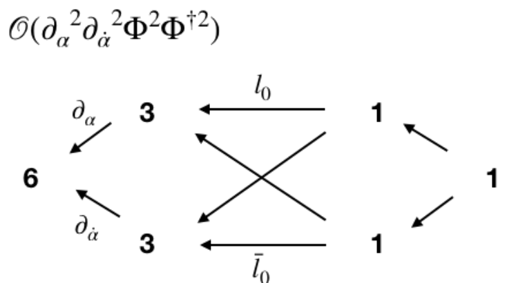
Consider the single flavor case with two chiral superfields and two anti-chiral superfields, i.e. . We want to find the operator basis for operator spaces in the form of , where is the number of superderivatives and . The first non-trivial space generated by operator in this form is the at dimension 6 when . It’s not difficult to see that there are 6 operators in the space modulo EOM, namely:
| (63) |
However, not all of them are independent under IBP relations. For example, the equation
| (64) |
indicates that the two terms on the right hand side are not independent, and as a result only one of them should exist in the operator space. Notice that terms like are dropped due to the EOM relations in the above equation. Since there are terms in and spaces, we can derive six IBP relations:
| (65) |
A brute force way to find the number of independent operators is to apply matrix rank approach, as in Ref. Lehman:2015coa. Specifically, we label each different element as and each relation provides an equation , where are the elements in each relation. For example the previous six relations can be transformed into a set of equations: . What’s left is to find the solution to this set of equations and the easiest way is to use a matrix solution. The rank of the matrix then gives the independent number of ’s. Rather than directly calculate the rank of the matrix relations for this example, we will proceed more methodically and check how the existence of previous (meaning fewer derivatives, so to the right in Fig. 2) spaces imply dependancies among the relations at each step along the way.
Applied to the case at hand, it seems like that the six relations will remove all six terms in the . However, this is not true because the six relations are not independent, and therefore we need higher order corrections coming from and . The relations we get from these two spaces are:
Clearly, the above relations are the same, so we should add 1 back instead of 2. The reason comes from the fact that the LHS of the above two equations comes from the term in , and therefore are corrected by :
| (66) |
Finally we add up the numbers: , which gives the correct number of independent operators. The tree diagram is given on the left in Fig 7.
Since there are only four superderivatives in this example, spaces transforming under larger representations are automatically null. However, once we consider operators with more superderivatives, those spaces must be taken into account. Non-vanishing larger representations are very common especially when we deal with multiple flavors, since in that case the constraints from Fermi statistics is weaker.
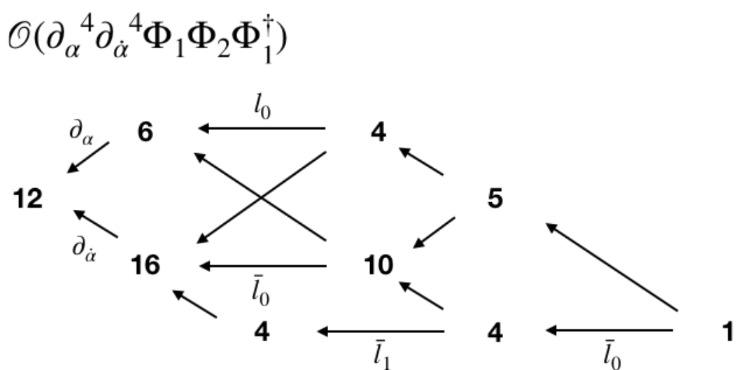
To illustrate this point, let’s take a look at the second example, involving two flavors and eight superderivatives, . We will not go into details to write down all orders of corrections, instead, we will compare the results we get from brute force way and our approach.
The tree diagram is shown on the right in Fig. 7. From IBP relations we get the following equations:
| (67) |
where is understood as , . We only list half of the 22 relations and the other 11 can be found by exchanging . Once one writes down all 22 relations, it becomes easy to calculate the rank of the giant matrix to find the number of independent terms. Plugged this into any math software, we find 0, exactly the same result you get by applying (62): .
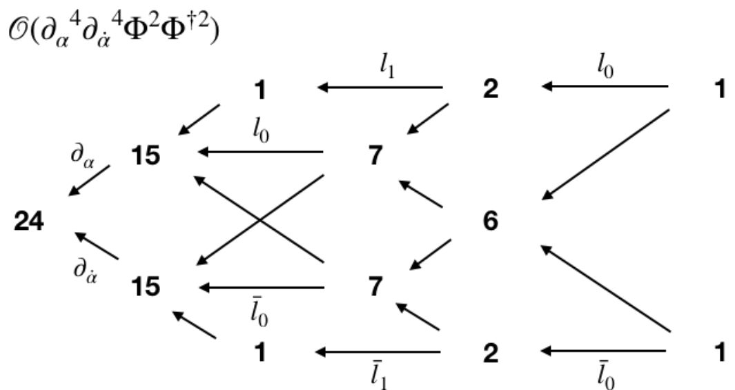
A third example is given in Fig. 8, where in this case we have four superfields and eight superderivatives. It is expected that as the dimension increases, the number of non-vanishing spaces increases, and the related tree diagram extends further. In this example, you can see that if one tries to find the number of independent operators, the dimension of the matrix is . As we add more and more superfields and superderivatives, the matrix becomes larger and is almost impossible for one to solve by brute force. Our approach provides a more accessible way since you no longer need to really find the matrix, instead you calculate the number of possible operators in each space, which can be easily done using Hilbert series. In this case we find invariants.
4 Conclusion and discussion
In this paper we have extended the technique of counting the number of independent effective operators to a supersymmetric theory with chiral superfields. Hilbert series and the plethystic exponential provide a way to form the full operator spaces, while EOM and IBP relations are removed by manipulating the characters and considering the correction spaces.
We find that supersymmetry, and in particular the presence of two, anticommuting derivatives, lead to interesting differences with respect to the non-supersymmetric case. The two superderivatives give two initial (‘zeroth order’) IBP relations, and the structure of the higher order IBP corrections becomes more complicated. We find the corrections organize themselves into six branches, grouped into one set of three oriented in the direction and a complex conjugate set oriented in the direction. All correction spaces satisfy a master relation, Eq. (41).
While a bit formal at first glance, we have seen that the interrelations among the maps implied by Eq. (41) are connected to relations between the two superderivatives and the ‘normal’ (or ‘bosonic’) derivative . As the superderivatives are fermionic, corrections spaces with multiple or indices are required to be symmetric in those indices. As there is no barrier to forming symmetric tensors of arbitrarily high dimension, the correction branches formally extend infinitely, though in practice they are cut by the number of derivatives in the operator we care about correcting. This can be contrasted with correction spaces in non-supersymmetric spaces, which must be antisymmetric in Lorentz indices and this truncate with regardless of how many derivatives the operator we want to correct has.
The full set of corrections can be resummed and turned into a prefactor, namely (61), , to insert into the Haar measure integral along with the plethystic exponential of the chiral/antichiral superfields of interest. This prefactor plays the role of the factor Henning:2017fpj in non-supersymmetric theories, and enacts the subtraction of IBP relations by projecting out and counting the appropriate correction spaces. For non-supersymmetric theories, Ref. Henning:2017fpj showed how the factor could be obtained by considering conformal symmetry as the organizing principle underlying how fields are combined, rather than Lorentz symmetry. The non-orthonormality of the (non-compact) conformal group characters, combined with integration over the dilatation portion of the Haar measure/Cartan subalgebra then yields . In that light, a natural question to ask is whether a generalization using superconformal representations reproduces . Naively one would expect to identify the two superderivatives as a representation of the supercharges – the additional fermionic generators in superconformal algebra – just as one treats the usual partial derivative as a representation of the momentum generator of the Poincare algebra. However, this identification fails: although the superderivatives do satisfy the same anticommutation relations, they are not simply the representation of supercharges. Recall the definition of superderivatives (9) and (10), from which we finds that superderivatives contain the usual partial derivative pieces. Formally one can write , where are supercharges and is the momentum generator. This realization indicates that and are interwined with the usual partial derivatives, which makes the superconformal approach much more complicated, and so far we have not succeeded in using it as a starting point.
Nonetheless, there is something we can learn from superconformal algebra, encoded in five independent vanishing (anti)commutators:
| (68) | ||||
The existence of the first branch makes use of the first identity, namely two consecutive superderivatives acting on symmetric indices automatically vanishes. To prove the existence of the second branch, we use the fact that superderivatives commutes with usual partial derivative, leading to the proof shown in (3.3.2). The last identity is essential to prove the maps indeed satisfy the requirement when we consider the third branch. To summarize, the vanishing of these special combinations of superderivatives leads to the existence of three correction branches, just as the fact that one branch exists in non-supersymmetric theories can be connected to the single vanishing commutator . Future studies on the relation between the method we develop here and the superconformal algebra is very promising and interesting.
We have only analyzed a supersymmetry chiral theory so the technique we developed here should be easily generalized to other supersymmetric theories. In a forthcoming publication we will apply what we learn to vector superfields, and postpone extended supersymmetric theories to later studies.
Acknowledgements.
We would like to thank Xiaochuan Lu for some useful comments on the draft. This work is partially supported by the National Science Foundation under Grant Number PHY-2112540.Appendix A Characters and Haar measures
Here we list a few characters in group and that are used in this paper. And we also list the related Haar measure for each group. For further characters, please refer to Hanany:2008sb.
The characters are given by:
| (69a) | ||||
| (69b) | ||||
| (69c) | ||||
where are related group parameters. In addition, the character of representation and are given by:
| (70a) | ||||
| (70b) | ||||
where are defined through , and are the related group parameters.
The Haar measures are given by:
| (71a) | ||||
| (71b) | ||||
| (71c) | ||||
Appendix B Proofs
B.1 Higher order corrections
In this Appendix, we show the detailed derivation leads to the explict form of coefficients in and given in (57). Recall the definition of acting on a definite representation, which is given by:
| (72) |
where is defined to be the fully symmetrization permutations of its indices. For example, .
These maps should satisfy the following equation such that the above correction spaces obey the definition, i.e. corrects and with respect to when :
| (73) |
Expand it using (72) and we get
| (74) |
Use the identity , we can rewrite the second term as:
| (75) |
where denotes that the indices do not contain the piece. We can separate it into two parts and compare their coefficients and solve for and . The two equations are given by
| (76) |
and
| (77) |
We can expand the symbol using the identity :
| (78) |
Put this back into the first equation, we get:
| (79) |
from which we can solve for and recursively:
| (80) |
The initial condition is given by and 1717 17 In principle the choice is not unique and one can always multiply this solution by a common factor. in order to generate the same define in Section 3.3.2. . Then we can solve and for general n:
| (81) |
We only make use of the first equation of (76) and (77). Now we need to prove that this solution does satisfy the second one (77):
| (82) |
follows from the fact that .
Futhermore, we require that 1818 18 This allows the horizontal composite maps to vanish by virtue of the definition of correction spaces., and the proof is straight forward.
| (83) |
Therefore to prove the above expression is 0, it suffices to prove the following equation
| (84) |
Expand the LHS and terms involving vanishes due to its antisymmetric property. In addition, we use the defining anticommutator to rewrite as . Finally we are left with
| (85) |
which identically vanishes. This completes the proof of .
B.2 Starting space of second branch
Here we answer the question arised at the end of 3.3.2, where one may wonder why the second branch starts from . The general solution to this problem is to consider the nearest spaces and check if they can satisfy the definition. If not, we need to move to the second nearest space and check again. Specifically, we know that gives the IBP relations, and the nearest spaces are and . The first one already exists in the first branch, while the second one cannot satisfy the definition. We can prove this by looking at the equation
| (86) |
If the space is indeed a correction, then we must find a nontrivial solution of the above equation. However this is impossible and therefore leads to contradiction. Then we do the same for the second nearest spaces and we find that when it transforms under , it satisfies the definition. The reason it doesn’t transform under is because in that case it leads to null space under the map and therefore cannot be a correction. Now we have completed the proof why the second branch starts from .
B.3 Infinite sum
References
- (1) B. Grzadkowski, M. Iskrzynski, M. Misiak, and J. Rosiek, “Dimension-Six Terms in the Standard Model Lagrangian,” JHEP 10 (2010) 085, arXiv:1008.4884 [hep-ph].
- (2) L. Lehman and A. Martin, “Hilbert Series for Constructing Lagrangians: expanding the phenomenologist’s toolbox,” Phys. Rev. D 91 (2015) 105014, arXiv:1503.07537 [hep-ph].
- (3) B. Henning, X. Lu, T. Melia, and H. Murayama, “Hilbert series and operator bases with derivatives in effective field theories,” Commun. Math. Phys. 347 (2016) no. 2, 363–388, arXiv:1507.07240 [hep-th].
- (4) L. Lehman and A. Martin, “Low-derivative operators of the Standard Model effective field theory via Hilbert series methods,” JHEP 02 (2016) 081, arXiv:1510.00372 [hep-ph].
- (5) B. Henning, X. Lu, T. Melia, and H. Murayama, “Operator bases, -matrices, and their partition functions,” JHEP 10 (2017) 199, arXiv:1706.08520 [hep-th].
- (6) Anisha, S. Das Bakshi, J. Chakrabortty, and S. Prakash, “Hilbert Series and Plethystics: Paving the path towards 2HDM- and MLRSM-EFT,” JHEP 09 (2019) 035, arXiv:1905.11047 [hep-ph].
- (7) C. B. Marinissen, R. Rahn, and W. J. Waalewijn, “…, 83106786, 114382724, 1509048322, 2343463290, 27410087742, … efficient Hilbert series for effective theories,” Phys. Lett. B 808 (2020) 135632, arXiv:2004.09521 [hep-ph].
- (8) L. Graf, B. Henning, X. Lu, T. Melia, and H. Murayama, “2, 12, 117, 1959, 45171, 1170086, …: a Hilbert series for the QCD chiral Lagrangian,” JHEP 01 (2021) 142, arXiv:2009.01239 [hep-ph].
- (9) Y. Wang, B. Yu, and S. Zhou, “Flavor invariants and renormalization-group equations in the leptonic sector with massive Majorana neutrinos,” JHEP 09 (2021) 053, arXiv:2107.06274 [hep-ph].
- (10) L. Gráf, B. Henning, X. Lu, T. Melia, and H. Murayama, “Hilbert Series, the Higgs Mechanism, and HEFT,” arXiv:2211.06275 [hep-ph].
- (11) B. Yu and S. Zhou, “Cp violation and flavor invariants in the seesaw effective field theory,”The journal of high energy physics 2022 (Aug 1,, 2022) 1–47. https://link.springer.com/article/10.1007/JHEP08(2022)017.
- (12) B. Yu and S. Zhou, “Spelling out leptonic cp violation in the language of invariant theory,” tech. rep., Cornell University Library, arXiv.org, Aug 25,, 2022. https://search.proquest.com/docview/2635121425.
- (13) B. Yu and S. Zhou, “Hilbert series for leptonic flavor invariants in the minimal seesaw model,”The journal of high energy physics 2021 (Oct 4,, 2021) 1–23. https://link.springer.com/article/10.1007/JHEP10(2021)017.
- (14) J. Lu, “(reply to) ”comment on ’flavor invariants and renormalization-group equations in the leptonic sector with massive majorana neutrinos’ ”,”. https://arxiv.org/abs/2111.02729.
- (15) J. Lu, “Comment on “flavor invariants and renormalization-group equations in the leptonic sector with massive majorana neutrinos”,”The journal of high energy physics 2022 (Feb 17,, 2022) 1–11. https://link.springer.com/article/10.1007/JHEP02(2022)135.
- (16) H. Sun, Y.-N. Wang, and J.-H. Yu, “Hilbert series and operator counting on the higgs effective field theory,”. https://arxiv.org/abs/2211.11598.
- (17) B. Henning and T. Melia, “Constructing effective field theories via their harmonics,” Phys. Rev. D 100 (2019) no. 1, 016015, arXiv:1902.06754 [hep-ph].
- (18) B. Henning and T. Melia, “Conformal-helicity duality \& the Hilbert space of free CFTs,” arXiv:1902.06747 [hep-th].
- (19) T. Ma, J. Shu, and M.-L. Xiao, “Standard Model Effective Field Theory from On-shell Amplitudes,” arXiv:1902.06752 [hep-ph].
- (20) G. Durieux and C. S. Machado, “Enumerating higher-dimensional operators with on-shell amplitudes,” Phys. Rev. D 101 (2020) no. 9, 095021, arXiv:1912.08827 [hep-ph].
- (21) Z.-Y. Dong, T. Ma, and J. Shu, “Constructing on-shell operator basis for all masses and spins,” arXiv:2103.15837 [hep-ph].
- (22) H.-L. Li, Z. Ren, M.-L. Xiao, J.-H. Yu, and Y.-H. Zheng, “Operators for generic effective field theory at any dimension: on-shell amplitude basis construction,” JHEP 04 (2022) 140, arXiv:2201.04639 [hep-ph].
- (23) R. M. Fonseca, “Enumerating the operators of an effective field theory,” Phys. Rev. D 101 (2020) no. 3, 035040, arXiv:1907.12584 [hep-ph].
- (24) H.-L. Li, Z. Ren, J. Shu, M.-L. Xiao, J.-H. Yu, and Y.-H. Zheng, “Complete set of dimension-eight operators in the standard model effective field theory,” Phys. Rev. D 104 (2021) no. 1, 015026, arXiv:2005.00008 [hep-ph].
- (25) B. Henning, X. Lu, T. Melia, and H. Murayama, “2, 84, 30, 993, 560, 15456, 11962, 261485, …: Higher dimension operators in the SM EFT,” JHEP 08 (2017) 016, arXiv:1512.03433 [hep-ph]. [Erratum: JHEP 09, 019 (2019)].
- (26) C. W. Murphy, “Dimension-8 operators in the Standard Model Eective Field Theory,” JHEP 10 (2020) 174, arXiv:2005.00059 [hep-ph].
- (27) A. Kobach and S. Pal, “Hilbert Series and Operator Basis for NRQED and NRQCD/HQET,” Phys. Lett. B 772 (2017) 225–231, arXiv:1704.00008 [hep-ph].
- (28) A. Gunawardana and G. Paz, “On HQET and NRQCD Operators of Dimension 8 and Above,” JHEP 07 (2017) 137, arXiv:1702.08904 [hep-ph].
- (29) Y. Liao and X.-D. Ma, “An explicit construction of the dimension-9 operator basis in the standard model effective field theory,” JHEP 11 (2020) 152, arXiv:2007.08125 [hep-ph].
- (30) H.-L. Li, Z. Ren, M.-L. Xiao, J.-H. Yu, and Y.-H. Zheng, “Complete set of dimension-nine operators in the standard model effective field theory,”Physical review. D 104 (Jul, 2021) 1. https://search.proquest.com/docview/2557548502.
- (31) I. Antoniadis, E. Dudas, and D. M. Ghilencea, “Supersymmetric Models with Higher Dimensional Operators,” JHEP 03 (2008) 045, arXiv:0708.0383 [hep-th].
- (32) D. Forcella, Master Space and Hilbert Series for N=1 Field Theories. PhD thesis, CNRS and Ecole Normale Superieure, Paris, 2008. arXiv:0902.2109 [hep-th].
- (33) F. Farakos, S. Ferrara, A. Kehagias, and M. Porrati, “Supersymmetry Breaking by Higher Dimension Operators,” Nucl. Phys. B 879 (2014) 348–369, arXiv:1309.1476 [hep-th].
- (34) E. Dudas and D. M. Ghilencea, “Effective operators in SUSY, superfield constraints and searches for a UV completion,” JHEP 06 (2015) 124, arXiv:1503.08319 [hep-th].
- (35) M. Nitta and S. Sasaki, “Higher Derivative Supersymmetric Nonlinear Sigma Models on Hermitian Symmetric Spaces, and BPS States Therein,” Phys. Rev. D 103 (2021) no. 2, 025001, arXiv:2011.07973 [hep-th].
- (36) P. Pouliot, “Molien function for duality,” JHEP 9901 (1999) 021, arXiv:hep-th/9812015 [hep-th].
- (37) S. Benvenuti, B. Feng, A. Hanany, and Y.-H. He, “Counting BPS Operators in Gauge Theories: Quivers, Syzygies and Plethystics,” JHEP 0711 (2007) 050, arXiv:hep-th/0608050 [hep-th].
- (38) A. Butti, D. Forcella, A. Hanany, D. Vegh, and A. Zaffaroni, “Counting Chiral Operators in Quiver Gauge Theories,” JHEP 0711 (2007) 092, arXiv:0705.2771 [hep-th].
- (39) B. Feng, A. Hanany, and Y.-H. He, “Counting gauge invariants: The Plethystic program,” JHEP 0703 (2007) 090, arXiv:hep-th/0701063 [hep-th].
- (40) D. Forcella, A. Hanany, and A. Zaffaroni, “Baryonic Generating Functions,” JHEP 0712 (2007) 022, arXiv:hep-th/0701236 [HEP-TH].
- (41) F. Dolan, “Counting BPS operators in N=4 SYM,” Nucl.Phys. B790 (2008) 432–464, arXiv:0704.1038 [hep-th].
- (42) J. Gray, A. Hanany, Y.-H. He, V. Jejjala, and N. Mekareeya, “SQCD: A Geometric Apercu,” JHEP 0805 (2008) 099, arXiv:0803.4257 [hep-th].
- (43) A. Hanany, N. Mekareeya, and G. Torri, “The Hilbert Series of Adjoint SQCD,” Nucl.Phys. B825 (2010) 52–97, arXiv:0812.2315 [hep-th].
- (44) S. Benvenuti, A. Hanany, and N. Mekareeya, “The Hilbert Series of the One Instanton Moduli Space,” JHEP 1006 (2010) 100, arXiv:1005.3026 [hep-th].
- (45) Y. Chen and N. Mekareeya, “The Hilbert series of U/SU SQCD and Toeplitz Determinants,” Nucl.Phys. B850 (2011) 553–593, arXiv:1104.2045 [hep-th].
- (46) A. Hanany, N. Mekareeya, and S. S. Razamat, “Hilbert Series for Moduli Spaces of Two Instantons,” JHEP 1301 (2013) 070, arXiv:1205.4741 [hep-th].
- (47) D. Rodríguez-Gómez and G. Zafrir, “On the 5d instanton index as a Hilbert series,” Nucl.Phys. B878 (2014) 1–11, arXiv:1305.5684 [hep-th].
- (48) A. Dey, A. Hanany, N. Mekareeya, D. Rodríguez-Gómez, and R.-K. Seong, “Hilbert Series for Moduli Spaces of Instantons on 2/n,” JHEP 1401 (2014) 182, arXiv:1309.0812 [hep-th].
- (49) A. Hanany and R.-K. Seong, “Hilbert series and moduli spaces of U(N ) vortices,” JHEP 1502 (2015) 012, arXiv:1403.4950 [hep-th].
- (50) A. Hanany and R. Kalveks, “Highest Weight Generating Functions for Hilbert Series,” JHEP 1410 (2014) 152, arXiv:1408.4690 [hep-th].
- (51) S. Weinberg, The quantum theory of fields. Vol. 3: Supersymmetry. Cambridge University Press, 6, 2013.
- (52) H. Georgi, “On-shell effective field theory,” Nucl. Phys. B 361 (1991) 339–350.
- (53) F. A. Dolan, “On Superconformal Characters and Partition Functions in Three Dimensions,” J. Math. Phys. 51 (2010) 022301, arXiv:0811.2740 [hep-th].
- (54) F. A. Dolan, “Character formulae and partition functions in higher dimensional conformal field theory,” J. Math. Phys. 47 (2006) 062303, arXiv:hep-th/0508031.
- (55) F. A. Dolan and H. Osborn, “On short and semi-short representations for four-dimensional superconformal symmetry,” Annals Phys. 307 (2003) 41–89, arXiv:hep-th/0209056.
- (56) I. Affleck, M. Dine, and N. Seiberg, “Dynamical Supersymmetry Breaking in Four-Dimensions and Its Phenomenological Implications,” Nucl. Phys. B 256 (1985) 557–599.
- (57) K. A. Intriligator and N. Seiberg, “Lectures on supersymmetric gauge theories and electric-magnetic duality,” Nucl. Phys. B Proc. Suppl. 45BC (1996) 1–28, arXiv:hep-th/9509066.
- (58) L. Brizi, M. Gomez-Reino, and C. A. Scrucca, “Globally and locally supersymmetric effective theories for light fields,” Nucl. Phys. B 820 (2009) 193–212, arXiv:0904.0370 [hep-th].