Learning Physically Realizable Skills for Online Packing
of General 3D ShapesJournal: TOGCCS: Computing methodologies Shape analysis

Abstract.
We study the problem of learning online packing skills for irregular 3D shapes, which is arguably the most challenging setting of bin packing problems. The goal is to consecutively move a sequence of 3D objects with arbitrary shapes into a designated container with only partial observations of the object sequence. Meanwhile, we take physical realizability into account, involving physics dynamics and constraints of a placement. The packing policy should understand the 3D geometry of the object to be packed and make effective decisions to accommodate it in the container in a physically realizable way. We propose a Reinforcement Learning (RL) pipeline to learn the policy. The complex irregular geometry and imperfect object placement together lead to huge solution space. Direct training in such space is prohibitively data intensive. We instead propose a theoretically-provable method for candidate action generation to reduce the action space of RL and the learning burden. A parameterized policy is then learned to select the best placement from the candidates. Equipped with an efficient method of asynchronous RL acceleration and a data preparation process of simulation-ready training sequences, a mature packing policy can be trained in a physics-based environment within 48 hours. Through extensive evaluation on a variety of real-life shape datasets and comparisons with state-of-the-art baselines, we demonstrate that our method outperforms the best-performing baseline on all datasets by at least in terms of packing utility. We also release our datasets and source code to support further research in this direction 11 1 Datasets and source code available at https://github.com/alexfrom0815/IR-BPP..
Keywords:
irregular shapes, 3D packing problem, reinforcement learning, combinatorial optimization1. Introduction
Packing, finding an efficient placement of as many as possible objects within a designated volume, has garnered multidisciplinary research interests from combinatorial optimization (Martello et al. 2000; Seiden 2002), computational geometry (Ma et al. 2018; Hu et al. 2020) and machine learning (Zhao et al. 2022a; Hu et al. 2017). The famous Kepler conjecture, which considers the continuous packing of spheres in infinite spaces, was proved only recently (Hales et al. 2017) after more than four centuries. Even the discrete bin packing problem has been proven NP-hard (Hartmanis 1982). For 3D shape packing, most existing works consider simple object shapes such as cuboids (Martello et al. 2000), tetrahedra (Conway and Torquato 2006), or ellipsoids (Kallrath 2017). The more general problem of irregular shape packing, on the other hand, has received much less study, although being practically useful in many real application scenarios. In robotics, product packing robots (Wang and Hauser 2019; Shome et al. 2019; Wang and Hauser 2021; Yang et al. 2021) for logistics automation is an active research area. In computer graphics, irregular shape packing has been widely explored in UV atlas generation (Limper et al. 2018; Liu et al. 2019; Zhang et al. 2020), artistic puzzle design (Wang et al. 2021; Chen et al. 2022), 2D panel fabrication (Saakes et al. 2013), and 3D printing (Chen et al. 2015), with various constraints.
We focus on practically feasible robotic packing, namely Physically Realizable Packing (PRP). In particular, PRP combines two well-known robotic tasks, pick-and-place (Han et al. 2019) and irregular shape packing (Wang and Hauser 2019), while further requiring packed objects governed by physics dynamics. As illustrated in Fig. 1, our virtual problem setup involves a robot arm equipped with a sucker-type gripper. Irregularly shaped objects are transported by a conveyor belt in a planar-stable pose and move at a constant speed. The upper surface of the object is captured by a top-view camera and the robot can move this object above an up-looking camera to capture its bottom surface. We pursue an online setting (Seiden 2002) where the robot observes only the object coming in the next instead of the full sequence. After the robot releases each object at its planned configuration inside the target container, we use a full-fledged physics simulator (Coumans and Bai 2016), compatible with the standard Reinforcement Learning (RL) platform (Brockman et al. 2016), to determine the ultimate quasi-static poses of all objects and enforce physically realizable constraints. Our physics constraint accounts for both quasi-static and dynamic interactions between objects, generalizing the prior pile stability constraint (Wang and Hauser 2019) which only considers quasi-static interactions.
We propose a novel RL pipeline to train effective packing policies. The sequential nature of packing has stimulated several recent RL-based approaches (Hu et al. 2020; Zhao et al. 2021; Zhao et al. 2022a). Compared with manually designed heuristics (Karabulut and Inceoglu 2004; Ramos et al. 2016; Ha et al. 2017), RL is capable of learning complex application-side constraints from guided explorations. RL also bears the potential to outperform humans on both continuous and discrete decision-making problems (Mnih et al. 2015; Duan et al. 2016). However, prior RL-based approaches opt to factor out the continuous aspect of the problem and only learn a discrete packing policy, via assuming cuboid objects and omitting physics constraints. The continuous nature of the irregular shape packing calls for exploiting the full potential of RL through accounting for physics constraints. We contribute a practical algorithm to learn packing policies for irregular 3D shapes via overcoming a series of technical challenges.
First of all, learning effective packing policies is naturally a tough challenge. The complex irregular geometry and imperfect object placement due to physics dynamics together lead to huge solution space. Direct policy training through trial and error in such spaces is prohibitively data intensive. We instead propose a candidate action generation method to reduce the action space of RL as well as the learning burden. The candidates are the convex vertices of the (polygonal) connected regions within which the current object can be placed. We prove that these candidates are local optima that make the object tightly packed against the obstacles (the placed objects and the container). Our learned policy is then used to understand the geometry of the current object and choose the best placement from its corresponding candidates. This method significantly reduces the search space of RL and enables reliable learning of packing policies.
Both the geometry understanding and the candidate selection need a gazillion experiences collected through simulation. However, interaction with the simulation world is CPU-bound and is time-consuming, which leaves policies less trained per wall-clock time. Some abnormally slow instances also block the uniform training schedule. To this end, we propose to accelerate the training via an asynchronous sampling strategy. In particular, we decouple the training into a parallelized experience sampling process for non-blocking treatment and a separate learning process for continuously updating parameters. Our method allows a robust packing policy to be trained within 48 hours on a desktop machine.
In addition, RL algorithms should be trained with sufficient data variety to ensure the robustness of the learned policies. As compared with cubical shape packing, however, the variety of object shapes and poses for irregular shape packing is on a much higher level. We propose a data preparation process for generating sequences of simulation-ready objects each with a planar-stable pose. Working with a combination of several real-world and synthetic datasets, we create a packing problem generator emitting randomized, versatile, and faithful problem instances.
We have conducted extensive evaluations of our method on well-established datasets with various geometric characteristics. By comparing with a row of baseline algorithms, we demonstrate that our method significantly outperforms the best-performing baseline on all datasets by at least in terms of packing utility. Furthermore, we extend our method to the scenario of buffered packing, where the robot maintains a buffer for re-ordering objects, and show that higher packing quality can be achieved. Our contributions include:
- •
An effective and theoretically-provable placement candidate generation method for pruning the action space of RL, along with a learnable packing policy for candidate selection.
- •
An efficient, asynchronous, off-policy sampling strategy for accelerating packing policy training.
- •
A constructive PRP environment modeling realistic packing with a large object dataset and RL-compatible interfaces.
2. Related Work
Our work is built off of prior works on packing policy searches. Our problem is also closely related to other packing-related tasks in computer graphics and robotics.
2.1. Packing Policies
Being an NP-hard problem, various heuristic policies have been proposed for 2D (Lodi et al. 2002) and 3D (Ali et al. 2022) cubical object packing over time, without a single best performer. The transition of focus to irregular shapes is quite recent. Liu et al. 2015 (Liu et al. 2015) pack irregular 3D shapes using a Minimum-Total-Potential-Energy (MTPE) heuristic and prioritize shapes with the lowest gravitational center of height. Wang and Hauser 2019 (Wang and Hauser 2019) propose the Heightmap Minimization (HM) heuristic to minimize the volume increase of packed non-convex shapes as observed from the loading direction. Goyal and Deng 2020 (Goyal and Deng 2020) make their packing decision via the Bottom-Left-Back-Fill (BLBF) heuristic (Tiwari et al. 2010), which places an object in the bottom-most, left-most, and back-most corner. All these placement rules are manually designed based on specific observations, which limits their applicability. For example, the HM heuristic performs quite well for non-convex shape packing, since it aims to minimize space occupancy vertically. However, it cannot differentiate horizontal placements on a flat container, leading to sub-optimal cases demonstrated in Fig. 2a.
The latest efforts (Hu et al. 2017; Duan et al. 2019; Hu et al. 2020; Zhao et al. 2021; Zhao et al. 2022a) resort to machine learning, specifically RL, to automatically synthesize policies that work well on an arbitrary cubical shape packing task without human intervention. Early works (Hu et al. 2017; Duan et al. 2019; Hu et al. 2020), however, only learn the order of cuboids to be packed, while using separate heuristics or algorithms to compute the placement. More recent work (Zhao et al. 2021) learns the placement policy via predicting logits of discretized placement locations. The latest work (Zhao et al. 2022a) combines the merit of heuristic and learning-based policies using a candidate selection policy parameterization, having the policy rank a pre-defined set of candidate placements. Similar candidate selection approaches have been proven effective in a variety of robot manipulation tasks, including grasping (Mahler et al. 2016), object transferring (Zeng et al. 2020), and assembly discovery (Funk et al. 2021; Funk et al. 2022), where manually designed heuristics are used to prune sub-optimal actions and learned policies further selects promising ones. Our policy inherits these ideas with necessary modifications toward irregular shapes. A concurrent work is (Huang et al. 2023) which investigates a similar problem of learning-based irregular shape packing. Unlike their method which works with a large resolution-complete action space, we propose a candidate selection algorithm to pre-select a small discrete set of candidate placements. This makes our approach achieve faster training and better packing utility.

2.2. Packing in Computer Graphics
There is a handful of packing-related graphic problems, most of which involve irregular shapes and continuous decision variables. UV atlas generation, for example, minimizes the memory footprint by packing many texture charts into a single texture image. To generate high-quality textures, an algorithm needs to jointly optimize irregular chart shapes and their continuous packing placements. Early works (Lévy et al. 2002; Ray et al. 2003) nail down the two classes of decision variables in separate sub-stages. More recent works (Limper et al. 2018; Liu et al. 2019; Zhang et al. 2020) couple the two sub-stages by decomposing the charts for higher packing efficacy. Limper et al. 2018 (Limper et al. 2018) propose a heuristic strategy to iteratively cut charts into smaller ones and repack them using heuristics (Nöll and Strieker 2011). However, the shape of chart boundaries is pre-determined and cannot be modified during cutting. Liu et al. 2019 (Liu et al. 2019) and Zhang et al. 2020 (Zhang et al. 2020) propose to deform charts into rectangular patches and then adopt rectangular packing heuristics (Schertler et al. 2018). But their work is irrespective of the sequential nature of the packing problem, deforming chart shapes in a sub-stage.
A similar requirement to UV atlas generation arises in 3D printing, where the limited volume of commodity 3D printers requires large objects to be partitioned and/or repacked for printing efficacy. The packing plan can be further constrained for manufacturability and structure robustness. The first work (Luo et al. 2012) in this direction cuts large objects using the BSP-tree, such that each leaf node fits into the printing volume. They choose cutting planes from the object surface patches, essentially discretizing the continuous solutions. Luo et al. 2012 (Luo et al. 2012) select BSP-tree structures guided by a score function incorporating various constraints. However, their optimization strategy is myopic, i.e., using a horizon equal to one. Their follow-up work (Yao et al. 2015) further allows irregular part shapes to be locally optimized for structure robustness and collision resolution, and then packs the parts into the printing volume using local numerical optimization. As a result, Yao et al. 2015 (Yao et al. 2015) allow continuous optimization of both irregular object shapes and packing placements, but their optimizer is still myopic. A similar approach has been proposed by Ma et al. 2018, which only optimizes the final object placement result and neglects the packing process.
Our problem is closely related to these works by optimizing online placements for general 3D shapes. Modeling packing as a sequential-decision making problem, our method bears the potential of closing the sub-optimality gap as illustrated in Fig. 2b. A related work to ours is TAP-Net (Hu et al. 2020), which considers sequential object selection and packing problem in a discrete state-action space, assuming cubical objects and perfect placement without physics dynamics. Our method deviates from (Hu et al. 2020) in two important ways. First, we assume continuous object placements and physics realizability constraints. This is a much more realistic setting mimicking real-world packing problems. Our physics simulator allows uncertainty to be modeled, lifting the assumption of perfect policy execution. Second, our policy parameterization enables the RL algorithm to directly train the entire policy end-to-end, instead of only the object selection policy as done in (Hu et al. 2020), which is one reason for our superior performance over all existing baselines.

2.3. Packing in Robotics
Roboticists consider packing as a component in the pipeline of perception, planning, predicting, and control, rather than a standalone algorithmic problem. However, the progress in robotic packing tasks is relatively slow. This is because the robust execution of high-quality packing plans is extremely difficult due to the tiny spaces between objects. We are only aware of a few prior works (Wang and Hauser 2019; Shome et al. 2019; Funk et al. 2021) presenting full-featured packing systems. Wang and Hauser 2019 (Wang and Hauser 2019) use a robot arm with a sucker-type gripper to grab objects from top-down views. Their following work (Wang and Hauser 2022) further introduces a fallback strategy to shake the target container and create new open spaces for packing. Shome et al. 2019 (Shome et al. 2019) restart the sensing, motion planning, and control loop whenever failures are detected in the downstream stages. Both methods use simple heuristics to solve the underlying packing problem, with Wang and Hauser 2019 (Wang and Hauser 2019) relying on the heightmap minimization heuristic and Shome et al. 2019 (Shome et al. 2019) assuming known cubical object shapes and compatible target container sizes. Funk et al. 2021 (Funk et al. 2021) proposed a novel system that effectively assembles 3D objects into a predetermined structure. For the assembly task, however, their method only assigns the mechanical parts to pre-defined positions of the target structure, while we need to optimize the object poses to maximize the space utility.
In contrast, bin-picking (Mahler et al. 2016; Mahler and Goldberg 2017) can be robustly executed on robot hardware, because the target container is assumed to be much larger than objects, rendering packing unimportant. The bin-picking solutions (Mahler et al. 2016; Mahler and Goldberg 2017), though quite different from ours, share commonality with our policy design. Both methods assume the availability of a set of candidate actions, which is then ranked by a learning-based policy. Most recently, Zeng et al. 2020 (Zeng et al. 2020) and Huang et al. 2022 (Huang et al. 2022) bring the accuracy and generality of learning-based object transfer policy to another level by introducing equivalency. By factoring out the 2D rigid rotations from the neural network input-output space, learning becomes much more sample-efficient. We adopt a similar approach for factoring out rigid rotations during the forward calculation of packing policies.
3. Method
We introduce our online packing problem setup in Section 3.1 and formulate it as Markov Decision Process (MDP) in Section 3.2. To effectively solve this problem, we design a novel packing pattern based on candidate actions generated by a theoretically-provable method in Section 3.3. In Section 3.4, we describe our asynchronous RL algorithm for accelerating packing policy training in the physics simulation world. Extensions to buffered packing scenarios will be discussed in Section3.5. The pipeline of our learning-based algorithm is outlined in Fig. 3.
3.1. Problem Statement
Irregular shape packing problem considers a finite set of geometric objects . Each (in its local frame of reference) is of an irregular and possibly non-convex shape. Following the conventional Bin Packing Problem (Martello et al. 2000) (BPP), the target container takes up the space . The goal is to move as many objects into in a collision-free and physically realizable manner and maximize the packing utility:
| (1) |
where and are the volume of object and the container volume, respectively.

3.1.1. Environmental Setup
To mimic the real-world scenario of pick-and-place tasks, we assume that objects are stably laid on the conveyor belt moving at a constant speed, leaving the robot with a limited time window to pick up and place each into . Clearly, the time window size is a complex function of conveyor belt speed, robot motion speed, and various system delays. However, these factors can be tuned for different hardware platforms and are out of the scope of this work. We assume a fixed time window size, which allows us to model object packing as a sequential-decision problem. We postulate that the robot arm is equipped with a sucker-type gripper that can only pick and place an arbitrarily-shaped object from the top, as illustrated in Fig. 4, and that any object and any placement location in can be reached by the robot. The robot can also apply a 1D rotation of the gripper around the Z-axis (vertical), the same assumption is adopted in (Zhao et al. 2022a). Therefore, the space for robot decision is , consisting of a 3D position and an in-plane rotation. As compared with (Hu et al. 2020) where the virtual robot can grasp a box from its four sides, our assumptions limit robot mobility but make it more amenable to real-world deployment.
To make packing decisions, the robot is equipped with three RGB-D cameras to fully observe the packing environment (Fig. 1a). The on-conveyor camera captures the top surface of the incoming object while the on-container camera observes the continuous packing configurations inside the container. After picking up the incoming object, the robot moves it over a third, up-looking camera to capture its bottom surface (Fig. 4b), thus fully observing the geometry of the object and applying an additional transformation to pack it.
Different from those works which only optimize the final packing result (Ma et al. 2018), PRP also concerns the packing process, i.e., moving the objects into the container one by one. Since the robot can only observe one object at a time, our packing problem follows the online setting (Seiden 2002) where each object is placed without the knowledge of the next ones. No further adjustment, such as unloading or readjusting, will be allowed. The robot must make an immediate decision that accommodates the incoming object while optimizing the overall compactness of the in-container layout. Packing alone is already a difficult combinatorial optimization problem, the arbitrarily complex object geometry and the imperfect placement make this problem even more challenging with huge solution space. We resort to RL to learn this packing skill automatically through trial and error.

3.1.2. Stable Object Poses
As compared with BPP problems which only consider 6 axis-aligned orientations of cuboids, an irregular 3D object can have an arbitrary local-to-world orientation spanning the entire . However, we can adopt a mild assumption that objects are stably lying on the conveyor belt with force equilibrium. This assumption holds when the conveyor belt has sufficient frictional forces and moves reasonably slowly, which is generally the case. We denote the incoming object id at the th timestep as . Mathematically, is subject to a world transform such that is a physically stable pose on the conveyor belt as Fig. 5a. The robot can then apply a vertical rigid transformation such that and is collision-free with the boundary of or any other objects already in , as shown in Fig. 5b. Here is the vertical rotation angle and the 3D target position which takes the Front-Left-Bottom (FLB) of the Axis-Aligned Bounding Box (AABB) of as the reference point. Finally, the robot releases with and the ultimate continuous configurations of all placed objects , denoted as , are governed by rigid body physics dynamics like Fig. 5c.
3.2. PRP Learning Environment
In this section, we discuss our PRP environment compatible with all statements of Section 3.1. This involves a random packing problem emission procedure and an environment model that casts online packing as a Markov Decision Process for RL training.
Problem Emission
We aim at learning packing skills for 3D shapes of a specific data distribution, so the training and testing sequences are generated with objects from the same object dataset. The sequences are randomly generated and are not shared by training and testing. Although this is a typical assumption by most policy learning works, we will demonstrate the generalization of our method to out-of-distribution objects in Section 4.4. Given a shape set, we emit a random packing problem (a sequence of posed objects) by first picking a random shape from the dataset and then selecting a stable pose for it, both with uniform probability and bootstrap sampling. Then, the vertical in-plane orientation of an object is also uniformly randomized. The sampling is repeated until the objects of the sequence are enough to fill the container ().
Markov Decision Process
Our online packing problem can be formulated as a Markov Decision Process, which is a tuple . During each step of the decision, an agent observes the (partial) state of the current environment and makes a decision , where and are the state space and the action space, respectively. The environment then responds by bringing to via a stochastic transition function and granting a reward . The agent is modeled as a policy function , where is the observation function and the parameter of . Under this setting, solving the online packing problem amounts to the following stochastic optimization:
| (2) |
where is the stochastic problem emitter, is a constant discount factor, and is a sampled trajectory. Below we postulate each component of our MDP, putting together to form our packing environment.
State Space and Transition Function
At timestep , the true state of the current environment involves ultimate object configurations inside the target container and the state of the incoming object, i.e.:
essentially mimicking the online packing setting. The robot applies a temporary, initial transform for the th object. After that, our transition function, aka., the rigid body simulator (Coumans and Bai 2016), then integrates the poses of all objects to reach force equilibrium. We decide that all objects have reached force equilibrium when they have a velocity magnitude smaller than some threshold. At the force equilibrium state, we check for any objects that fall outside or have a height beyond , in which case we terminate the episode.
Observation Function o
We provide enough RGB-D cameras for capturing continuous object configurations inside container and the top/bottom surface of the incoming object . We assume that the captured RGB-D images have been segmented into foreground objects and background. We discard all color details and only retain the depth information. We further extract the heightmap of container with resolution , where is a regular interval. And we get a surface point cloud belonging to . We thus define our observation function as , which is also illustrated in Fig. 3ab.
Action Space
As mentioned in Section 3.1, the space for robot decision spans the entire , involving desired packing position and vertical orientation of the th object. We can naturally omit the -dimension decision because of the top-down placement manner. Typically, a robotic hardware platform such as (Pan and Hauser 2021) is equipped with force sensors and can determine the opportune time for releasing an object once collisions are detected. Therefore, no height measurement is needed for the object. Similarly, once the bottom object surface and the container heightmap are captured, we can get the object’s landing altitude when being placed at coordinates (Wang and Hauser 2019) and we denote as a function . Our packing policy only needs to figure out horizontal positions for given vertical rotation , essentially reducing the action space to . We define our action as , where is optional.
However, the space is still unaffordable for the sequential-decision nature of packing. For enabling efficient and effective policy learning, we propose to prune this enormous action space to limited placement candidates via a geometric-inspired method and use a parameterized policy to further select the best one. Our motivation and implementation of this candidate-based packing pattern will be deferred to Section 3.3.
Reward Signal R
Since we aim to maximize the packing utility in Equation 1, we directly grant a reward proportional to the volume of once is successfully placed inside the container. Here is a constant weight. Otherwise, the reward is zero and the trajectory is terminated. To avoid premature trajectory termination and get more step-wise profits, the agent should learn to optimize the packing process for accommodating more future possible objects.
3.3. Candidate-Based Packing Pattern
In this section, we introduce our packing policy representation, including a theoretically-provable candidate action generation method and a learnable policy for further candidate selection.
3.3.1. Candidate Action Generation
An intuitive attempt for acting in the space is discretizing it using a regular interval, as done in (Goyal and Deng 2020; Huang et al. 2023). However, this leads to a large action space which also grows exponentially with higher resolutions and larger container sizes. Meanwhile, the clustered actions with close distances also result in meaningless RL exploration. Generating an effective action subset with a controllable size is necessary for efficient packing policy learning which is also verified in (Zhao et al. 2022b) for cuboid packing.


Given an object to be packed, we hope to find a finite set of candidate actions that result in the object being tightly placed against the obstacles (container boundary or already placed objects) and permit no further movement, so that maximum empty room is left unoccupied for future object packing. See a counter-example in Fig. 6a. However, the irregular 3D boundaries of already packed objects can significantly complicate the analysis of candidate actions. To simplify the analysis, we consider the 2.5D top-down height field formed by the packed objects. We first extract near-planar connected regions formed by areas of similar values. We then consider the boundaries of the projected 2D regions. To ensure compact packing, we assume that the object should be placed at a (locally) convex vertex of a 2D connected region (Fig. 6b), with which we can obtain a discrete set of candidate actions for the object. To provide a theoretical validation, we prove the following 2D theorem:
Theorem 3.1.
For a 2D (polygonal) connected region and a point on its boundary , if is a convex vertex, then for an open neighborhood of which does not contain any other convex vertices and a tightness measure .
We define the tightness measure as the range of directions making touch the obstacles and permit no further movement, where is Minkowski sum (Mark et al. 2008) and we vertically rotate with to get . See Fig. 7 for the explanation of this definition. We provide a proof of this theorem in the next subsection. Essentially, this theorem claims that a convex vertex of is a local optimum that leads to a tight object packing (see Fig. 6c) which can be chosen as an action of the candidate. We extract candidate actions from all . We employ RL policies to further rank these locally optimal candidate actions and make globally optimal decisions. This strategy effectively reduces the dimension of action space.
3.3.2. Rationale of Candidate Generation Method
We will formally define our tightness measure and provide a proof of Theorem 3.1. Given a 3D object with known orientation, we can project it on the horizontal plane as a 2D polygon , so all the following analysis are restricted to 2D by projection. For example, we denote as the horizontal projection of packed objects. We can get feasible action regions which satisfy that and , where is Minkowski sum (Mark et al. 2008). With rotation fixed, the placement of reduces to selecting a reference point from and is the corresponding placement (see illustrations in Fig. 8ab).
We prefer point which places tightly against obstacles, for which there is no straightforward metric. Mark et al. 2008 define an extreme concept on polygons, one polygon is more extreme in a direction than another if its extreme points lie further in that direction. Inspired by this, we adopt which is the extreme value of ’s projection for the packing task. Placing at is more extreme than one placement in direction if is higher than . When is tightly packed against obstacles at along , also reaches a local maximal, as illustrated in Fig. 8c. Therefore, we get an intuitive indicator of tight packing, i.e.:
| (3) |
for some open neighborhood of and some direction . The following property is an immediate consequence of the Minkowski sum, which establishes a direct connection between packing tightness and reference points in :
Proposition 3.2.
If Equation 3 holds for some open neighborhood , then:
| (4) |
In other words, if is local optima, i.e. for all , the point corresponds to the most extreme placement of in its neighborhood. With this tool at hand, we can directly evaluate and compare the potential packing tightness of a point by looking at the range of directions that makes satisfy Equation 4.
Such a range of corresponds exactly to the spanning angle of a 2D normal cone (Boyd et al. 2004). The normal cone of a set at a boundary point is the set of all vectors such that for all . We summarize this property as our definition of tightness measure below:
Proposition 3.3.
For a convex polygonal set and , the spanning angle of the normal cone at is defined as our tightness measure , where is the interior angle of at .
A demonstration of a normal cone is provided in Fig. 9a. For a concave polygon, points located on its concave parts have no normal cone, and we extend that in this case, as shown in Fig. 9b. Using as a tightness metric, we compare different choices of . The proof for Theorem 3.1 is obvious:
Proof.
Normal cones only exist on boundary points of the polygon and not the internal ones. Therefore, we could consider a neighborhood containing and ’s two neighboring edges, without any other convex vertices included. Within , is convex so . All other points are on a straight line or concave vertices, with . ∎
We demonstrate some neighborhoods in Fig. 10. Each convex vertex corresponds to the local optima of and a tight object placement against obstacles. Based on the above observations, our candidate set consists of all convex vertices of the given .
3.3.3. Implementation and Policy Parameterization
Given a fixed in-plane rotation , we construct the candidate action set for using three steps. We firstly consider the full placement set which satisfy and , for . We discretize the container into regular grids and sample grid points lying in . Next, we detect and cluster all feasible, connected 2D regions from discretized positions, where each results in placed with similar altitudes, see also Fig. 6a. We denote two neighboring grids and as connected if:
| (5) |
with being a constant parameter. As our third step, for each connected region , we draw the region contour (Suzuki and Abe 1985) where touches the container boundary or packed objects from the top-down view. Since contours are pixelized, we approximate to polygons with the Ramer-Douglas-Peucker algorithm (Ramer 1972) and detect convex polygon vertices as candidate FLBs (Fig. 6b). We execute this procedure for all possible in-plane rotations discretized at a regular interval of . Finally, the number of candidate FLB positions can be large, and we sort them by in ascending order and retain the first . We outline the candidate generation details in Algorithm 1. Our candidate generation procedure imposes no requirement on object geometry and fits the general shape packing need.
Given the packing observation tuple and the generated candidate actions, our packing policy is used to understand 3D task geometry and rank candidates for selection. Our policy first encodes the container heightmap by a Convolutional Neural Network (CNN) to extract feature . Similarly, we use a PointNet architecture (Qi et al. 2017) to project the point cloud to feature . Both feature extractors are designed lightweight and trained from scratch. We apply a vertical transform to the point cloud until its AABB has the smallest volume with FLB at the origin. This essentially follows a similar idea to (Zeng et al. 2020) which transforms the point cloud to a canonical pose to improve data efficiency. The th candidate action is brought through an element-wise Multi-Layer Perceptron (MLP) to derive a candidate descriptor . Our candidate selector then takes the same form as a standard dueling Q-network (Wang et al. 2016), which is also illustrated in Fig. 3. This architecture represents the state-action value function as:
where is the number of candidate actions. is called the state value function and is the advantage function. We concatenate and parameterize the problem features to and with two MLPs, with learnable parameters and , respectively:
Our ultimate action is defined as:
The number of candidate actions accepted by our policy is fixed to . If the factual number of candidates is less than , we fulfill the candidate array with dummy actions that are all-zero tuples. The Q-value predictions for these redundant candidates are replaced with during action selection.
3.4. Asynchronous Policy Training in Simulation World
Aside from that the complex irregular geometry and imperfect object placement enlarge the combinatorial solution space of packing, the heavy cost of exploring this enormous solution space, i.e. physics simulation, also makes it more difficult to learn an effective packing policy. In this section, we discuss several practical approaches to improve the efficiency of exploration and policy training in the simulation world. We choose a data-efficient off-policy RL algorithm and further use an asynchronous pipeline for accelerating the training, where the simulation-intensive trajectory sampling and policy optimization are performed asynchronously; a partial simulation further lowers the sample cost.
Existing reinforcement learning algorithms can be largely divided into on-policy approaches (Schulman et al. 2017; Wu et al. 2017) and off-policy methods (Barth-Maron et al. 2018; Wang et al. 2016). The former maximizes the expectation in Equation 2 by sampling trajectories using the current policy, while the latter maintains an experience memory that stores trajectories sampled using out-of-sync policies. Off-policy methods minimize the Bellman loss using samples from :
The ability to reuse samples makes off-policy algorithms more data-efficient, which is critical to our problem. As mentioned in Section 3.3, we use dueling networks (Wang et al. 2016) to allow more frequent updates of and share the learning across multiple candidate actions. We adopt the discrete action space DRL algorithm — Rainbow (Hessel et al. 2018) to train the dueling networks. Besides the dueling architecture, the Rainbow algorithm also fruitfully combines the well-known DQN method (Mnih et al. 2015) with other five independent improvements like prioritized replay (Schaul et al. 2016), noisy nets (Fortunato et al. 2018), distributional Q-learning (Bellemare et al. 2017), and so on.
3.4.1. Asynchronous Rainbow
In the vanilla Rainbow algorithm, the experience collection step and the policy learning step run alternatively, as demonstrated in Fig. 11a. For our problem, however, experience collection via physics simulation is CPU-bound and time-consuming, which leaves policies less trained. Given that the policy learning is merely GPU-bound, we propose to parallelize training via an asynchronous scheme similar to (Horgan et al. 2018). Specifically, we create an actor and a learner residing in two different processes, as illustrated in Fig. 11b. The actor interacts with the packing environment and collects experience. The collected data is saved to a memory which is shared between processes. The learner keeps learning from and spontaneously updates the actor with the latest parameters. Our asynchronous implementation not only saves wall-clock training time but also accesses higher-quality experiences by having the actor refine its parameter more frequently before each decision.
To further accelerate the experience collection step, we run multiple simulation threads along with a non-blocking treatment in the actor process. There are two-fold benefits of doing so. First, more sampling threads enrich experiences for policy learning. Moreover, the batched simulation also avoids the uniform training schedule being blocked by abnormally slow instances, as exemplified in Fig. 11a. Such abnormality can happen when the physical simulator is unstable and experiences a sudden gain in kinetic energy, requiring many more timesteps to converge to a new equilibrium configuration. We suspend the actor thread whenever its reaction time is longer than a threshold, as demonstrated in Fig. 11b. This suspended thread will then be treated as a standalone instance and rejoin others after its task is finished. This implementation guarantees sufficient concurrency in trajectory sampling.
3.4.2. Partial Simulation
Even by using asynchronous Rainbow, the policy training for PRP is still bound by the massive simulation cost. We can further accelerate training by fixing the configurations of already packed objects. In practice, we find that old objects are not affected much by new arrivals. Using this strategy can save a large portion of simulation costs. It can also save the price of computing heightmap , since we only need to update the slice of covered by the newly arrived object but scan the entire container. This simple strategy can significantly boost the simulation frequency by more than three times. Note that this partial simulation is only used during training, and we always simulate all objects and scan the entire container at test time for practicality.
3.5. Extension to Buffered Packing Scenario
So far we have discussed the strictly online packing problem. In some real-world scenarios, a buffered area can be used to temporarily store objects before the final placement, as shown in Fig. 12. By introducing the buffer, the robot can reorder objects locally before packing, potentially improving the packing performance by enabling a much larger search space. We suppose the buffered area is of a fixed size . When a new object comes, the robot will store this object in . If there are already objects inside , the robot will pass on one of the objects from to . Solving this problem not only involves reasoning about the picked object geometry, but considering the permutation of objects inside the buffer and future possible ones as well. To this end, we use an additional policy to select objects from , which is followed by our packing policy in Section 3.2. The area of is sufficiently large such that objects can be placed horizontally, and the point cloud feature of each object in is stored and available to . Finally, we assume the robot can reach any position in the buffered area from a top-down view.
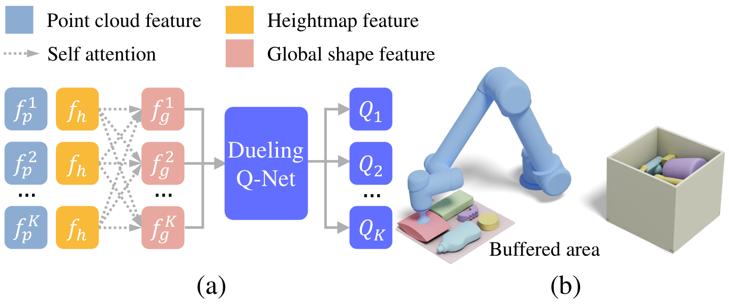
Our architecture of is illustrated in Fig. 12a. We assume there are objects in the buffer, denoted as , with their point clouds being . Similar to Fig. 3, our policy first maps each to a feature in an element-wise manner and maps the container heightmap to a feature . We adopt a Graph Attention Network (GAT) (Velickovic et al. 2018) to project the tuple to a high-level element feature . A dueling Q-network block is then used to select the best object with , where is the average of all features. We train the object-ordering policy and the placement policy jointly in an end-to-end manner. That is, first chooses one shape , then it is ’s turn to cooperate and choose a candidate action for placing .
4. Results and Evaluation
In this section, we first explain our packing experiment setup. Then, we describe our carefully prepared datasets emulating realistic packing tasks in Section 4.1. We illustrate the superiority of our method for online packing by comparing it with a row of existing baselines in Section 4.2 and demonstrate the benefits of our candidate-based packing pattern in Section 4.3. We report the generalization results of our method in Section 4.4, where the problem emitter transfers to noisy point cloud inputs and unseen shapes. Immediately following, we show performance on buffered packing scenarios in Section 4.5.
We establish our packing environment using the Bullet simulator (Coumans and Bai 2016), with a deep container of size cm, cm, and cm following Wang and Hauser 2019. We assume all objects have the same uniform density for estimating the center of mass. The coefficients of friction among objects and against the container are both set to . We set the grid size of the heightmap to be cm. We then sample at an interval of grids to form grid points for the candidate generation procedure. For clustering the connected region with similar values, we use cm. Unless otherwise stated, we use to discretize object rotations. We use a maximum of candidate actions for policy ranking. Our PointNet takes a fixed-sized set of points, so we resample points from the surface point cloud to fit this size. We adopt simulation threads in the actor process and set the discount factor for training. The training process is conducted on a desktop computer equipped with a Xeon E5-2620 CPU and a TITAN Xp GPU. Our learning-based policies are optimized within 48 hours with a maximum of 9.6 million interactions with the packing environment. Further analysis of the effects of these experimental parameters and training methods is provided in Appendix B.

4.1. Object Data Preparation
For training reliable policies for packing irregular 3D shapes, we need to prepare object datasets that contain abundant shapes as well as their planar-stable poses, while being compatible with the simulator. Our object test suite combines objects from widely used, open-source polygonal mesh (Botsch et al. 2010) datasets, collected either by synthetic modeling or real-world scanning.
To perform robust collision detections and ray-casting tests in the simulation world, we stipulate that objects are represented as closed manifold mesh surfaces. For each object, we first use the method in (Stutz and Geiger 2020) to reconstruct the mesh into a watertight one. We then extract all the planar-stable poses using the detection algorithm (Goldberg et al. 1999), as explained in Fig. 13a. Some planar-stable poses are rotation-symmetric as shown in Fig. 13b and we propose Algorithm 3 in Appendix A to remove redundant poses and retain only one representative from each rotation-symmetric group. This step avoids unbalanced shape distributions and improves the robustness of trained policies.

Finally, several rigid body simulators only accept convex shape primitives, e.g., approximating a non-convex power drill shape with its convex hull in Fig. 14a (red). We thus apply the convex decomposition algorithm (Mamou et al. 2016) for non-convex shapes, as illustrated in Fig. 14b. The complete data preparation pipeline is outlined in Algorithm 2 of Appendix A. The packing result or the final packing utility is highly related to the geometric properties of the picked object dataset. For providing convincing evaluations, we apply our pipeline to construct three datasets of various features.

General is a large dataset made up of daily life objects, as illustrated in Fig. 15a. It combines shapes from the KIT dataset (Kasper et al. 2012), the BigBIRD dataset (Singh et al. 2014), the GD dataset (Kappler et al. 2015), the APC dataset (Rennie et al. 2016), and the YCB dataset (Çalli et al. 2017), totalizing 483 shapes and 1094 planar-stable poses. All these shapes are collected through real-world scanning. General is our main dataset for profiling the performance of different methods.
BlockOut is a synthetic 3D puzzle dataset with polyominos that comes from Lo et al. 2009. This dataset includes 8 polyominos with 23 planar-stable poses, as illustrated in Fig. 15b. Each polyomino is composed of basic cubes of the same size. This dataset involves relatively regular shapes that are more complex to handle than cubical objects in BPP problems. BlockOut demonstrates the algorithm’s ability to understand shapes and combine them, as done in Fig. 2.
Kitchen consists of three categories of shapes, namely bowl, board, and fruit. The bowl shapes are concave CAD models collected from the ShapeNet dataset (Chang et al. 2015), as illustrated in Fig. 15c. The board shapes are manually created by us and the fruit shapes are small items coming from the General dataset. This dataset is created in order to verify a commonsense logic: an effective packing method would try to place fruits in bowls before covering boards. We expect the learned policies to pick up such logical rules without human intervention thus achieving better packing performance.
We compose the polyominos in the BlockOut dataset with basic cubes with a side length of cm. Therefore, the upper packing utility bound for the chosen container is . The rotation interval for BlockOut is set to since the polyomino shapes are axis-aligned. To construct the Kitchen dataset, we collect 54 concave bowl shapes from the ShapeNet dataset, 106 fruits from the General dataset, and 20 planar boards generated with random sizes. The problem emitter for the Kitchen dataset is slightly different from the others. Since we focus on verifying the packing logic between shape categories, we first sample an object category and then sample a random object with its most stable pose from this category. We also provide experimental results on industrial shapes collected from the ABC dataset (Koch et al. 2019) in Appendix B.

4.2. Comparisons with Heuristic Baselines
We compare our learned policies with several representative heuristic methods that can pack irregular 3D shapes. The MTPE heuristic (Liu et al. 2015) searches for the pose with the lowest center-of-mass height. The HM heuristic (Wang and Hauser 2019) endeavors to minimize the volume increase as observed from the top-down direction. The BLBF (Goyal and Deng 2020) heuristic selects the bottom-most, left-most, and back-most placement. We also test a classic First-Fit (FF) (Falkenauer 1996) packing logic which places items in the first found feasible placement.
We run all methods in the same environment setup with the same test sequences. A total of object sequences, randomly generated from each dataset, are tested. The performance of these baselines is assessed across five distinct metrics. We designate the packing utility as for each test sequence, which is the volume of packed objects divided by the volume of container . We report the average utility to reflect the overall performance of each method. With the exception of the BlockOut dataset where all shapes are composed of regular cubes, optimal packing solutions for other datasets are hard to derive. Consequently, we provide the utility gap against the best baseline. In particular, we calculate to highlight the performance discrepancy. Here denotes the average utility of the best performer, which is consistently our method. We also list the utility variance and the average number of packed objects. Lastly, we present the average computational time for solving each packing problem.
| General | BlockOut | Kitchen | |||||||||||||
| Method | Uti. | Gap | Var. | Num. | Time | Uti. | Gap | Var. | Num. | Time | Uti. | Gap | Var. | Num. | Time |
| Random | 31.6% | 29.0% | 5.8 | 19.6 | 0.03 | 37.1% | 47.7% | 3.4 | 17.8 | 0.02 | 22.6% | 42.3% | 6.4 | 16.7 | 0.03 |
| Random | 32.9% | 26.1% | 4.6 | 20.4 | 0.04 | 42.1% | 40.7% | 3.5 | 20.2 | 0.02 | 25.8% | 34.2% | 5.5 | 18.9 | 0.03 |
| FF (Falkenauer 1996) | 36.2% | 18.7% | 4.6 | 22.2 | 0.03 | 43.0% | 39.4% | 4.0 | 20.6 | 0.02 | 26.4% | 32.7% | 6.3 | 19.3 | 0.03 |
| MTPE (Liu et al. 2015) | 37.3% | 16.2% | 4.6 | 22.7 | 0.04 | 58.4% | 17.7% | 3.6 | 27.9 | 0.02 | 32.2% | 17.9% | 5.1 | 23.4 | 0.03 |
| HM (Wang and Hauser 2019) | 35.8% | 19.6% | 4.8 | 21.8 | 0.03 | 59.5% | 16.2% | 3.7 | 28.4 | 0.02 | 32.6% | 16.8% | 5.4 | 23.7 | 0.03 |
| BLBF (Goyal and Deng 2020) | 36.6% | 17.8% | 4.6 | 22.7 | 0.03 | 61.9% | 12.8% | 4.1 | 29.5 | 0.02 | 32.0% | 18.4% | 5.2 | 23.3 | 0.03 |
| Ours | 44.5% | 0.0% | 3.4 | 27.7 | 0.04 | 71.0% | 0.0% | 1.7 | 34.8 | 0.02 | 39.2% | 0.0% | 4.5 | 29.4 | 0.03 |
The quantitative and qualitative comparisons are summarized in Table 1 and Fig. 16, respectively. The best-performing heuristic for each dataset differs due to their distinct geometric properties. For instance, MTPE has an advantage on the General dataset, while HM is the best heuristic for the Kitchen dataset which has relatively more non-convex shapes. Compared to these manually designed packing rules, our learned policies adapt well to each dataset and consistently dominate heuristic rules. The gap metric demonstrates that our method outperforms even the best-performing baseline on each dataset with at least 12.8% in terms of packing utility. All these methods meet real-time packing requirements with a framerate of at least . Moreover, our method achieves the least variance on each dataset, further attesting to its robustness. More packing visualizations are provided in Appendix B for a more detailed understanding. We have also incorporated a dynamic packing video in the supplemental material for a comprehensive perspective.
During the packing process, the number of candidate actions can be large. The cardinality of the candidate set is outlined in Table 2. In order to mitigate the computational burden, we feed at most candidate actions to the policy network for each decision. As demonstrated in Table 1, we can see that randomly selecting a candidate action (Random ) outperforms picking a random resolution-complete action, while applying our learned policies to rank these locally optimal candidate actions enhances the packing performance even further. We have also compared with the baseline that randomly selecting an action from all the candidates (instead of limiting to at most ). The outcomes are comparable, yielding a performance of 32.9% for General, 42.2% for BlockOut, and 25.5% for Kitchen.
| General | BlockOut | Kitchen | ||||
| Method | Mean | Max | Mean | Max | Mean | Max |
| Ours | 195.7 | 868.0 | 51.0 | 172.0 | 140.3 | 605.0 |
4.3. Benefits of Candidate-based Packing Pattern
One of our main contributions lies in action space design, i.e., the candidate-based packing pattern for pruning sub-optimal actions. We highlight the effectiveness of our design in this section. We first compare with the resolution-complete action space, which discretizes the action space using a regular interval as done in (Goyal and Deng 2020; Huang et al. 2023). This action space can also be treated as a full geometry set including convex vertices, concave vertices, edges, and internal points of connected action regions, which would demonstrate the functionality of our generated candidates. Then, we also compare with other dimension-reduction techniques below.
| General | BlockOut | Kitchen | |||||||||||||
| Action Space Design | Uti. | Gap | Var. | Num. | Time | Uti. | Gap | Var. | Num. | Time | Uti. | Gap | Var. | Num. | Time |
| Resolution-Complete | 41.6% | 6.5% | 5.0 | 26.4 | 0.04 | 55.7% | 21.5% | 3.4 | 27.7 | 0.02 | 32.7% | 16.6% | 5.2 | 25.5 | 0.03 |
| Act in Line | 42.2% | 5.2% | 4.4 | 26.8 | 0.03 | 60.3% | 15.1% | 2.7 | 29.9 | 0.02 | 34.9% | 11.0% | 4.2 | 27.1 | 0.03 |
| Act on Orientation | 38.6% | 13.3% | 5.2 | 24.6 | 0.03 | 57.6% | 18.9% | 3.6 | 28.5 | 0.02 | 32.1% | 18.1% | 5.6 | 25.1 | 0.03 |
| Act on Heuristics | 40.1% | 9.9% | 6.0 | 25.5 | 0.03 | 65.4% | 7.9% | 2.6 | 32.2 | 0.02 | 32.8% | 16.3% | 5.6 | 25.4 | 0.03 |
| Ours | 44.5% | 0.0% | 3.4 | 27.7 | 0.04 | 71.0% | 0.0% | 1.7 | 34.8 | 0.02 | 39.2% | 0.0% | 4.5 | 29.4 | 0.03 |
Act in Line. The resolution-complete action space for packing is typically large and sensitive to the container size and the related intervals for discretizing the space . We can get the scale of this discretized space . To sidestep such an enormous space that can grow explosively, we only require the robot to provide and . The position can be determined via for given , thus reducing the action space to with .
Act on Orientation. Along the same line of thinking, we can further reduce the action space by only asking the robot to output and determine via . Thus reducing the action space to with .
Act on Heuristics. Since heuristic methods have different packing preferences, a straightforward packing strategy is to select one of the heuristics for the object to be packed. We collect all heuristics mentioned in Section 4.2 as a candidate action set m. The action space size, in this case, is .
For all alternatives mentioned above, we replace Q-values of invalid actions with negative infinity () during the decision-making process, and the subsequent performances are collated in Table 3. The widely adopted resolution-complete design of the action space (Goyal and Deng 2020; Huang et al. 2023), i.e. utilizing a brute-force discretization of 2D translation and rotation to form the action space, performs notably inferior to our method across all datasets. The reasoning behind this lies in the large action space, which necessitates extensive RL exploration and exceeds feasible computational capacity.
Gaining advantages from dimension reduction, Act-in-Line consistently outperforms resolution-complete actions. However, if we further reduce the action space to , i.e., Act-on-Orientation, the decision flexibility decreases and correspondingly, the performance degrades. Unsurprisingly, Act-on-Heuristics surpasses the performance of each individual heuristic reported in Table 1. However, the packing behavior of the learned policy is still restricted by basic heuristic components, and consequently, the improvements are limited. In comparison, our method stands out as the consistently best performer by reducing the action space to candidate actions of a fixed size . This approach not only alleviates the learning burden but also enables compact object packing.
4.4. Generalization Ability
The generalization capability of learning-based methods, i.e., testing the trained policies with a problem emitter differing from the training one, has always been a concern. Here we demonstrate our generalization proficiency with two experiments from practical perspectives.
Generalization on Noisy Point Clouds
We utilize a point cloud to represent the incoming object, which is then re-sampled randomly from . To exhibit our generalization capability, we apply Gaussian noises to the re-sampled . Here represents the standard deviation and is the diagonal length of ’s AABB. Then we generalize the policies trained on to .
Generalization on Unseen Shapes
To examine our method’s performance on unseen shapes, we randomly exclude of shapes from each dataset for training and we test the trained policies on the complete datasets afterwards. For the Kitchen dataset, this shape removal is executed by each category.
| General | BlockOut | Kitchen | |||||||
| Noise | Uti. | Var. | Num. | Uti. | Var. | Num. | Uti. | Var. | Num. |
| 44.5% | 3.4 | 27.7 | 71.0% | 1.7 | 34.8 | 39.2% | 4.5 | 29.4 | |
| 44.5% | 3.5 | 27.7 | 70.7% | 1.7 | 34.7 | 38.8% | 4.5 | 29.0 | |
| 44.4% | 3.4 | 27.6 | 70.7% | 1.7 | 34.7 | 38.9% | 4.3 | 29.1 | |
| 44.3% | 3.4 | 27.6 | 70.5% | 1.8 | 34.6 | 38.5% | 4.5 | 28.9 | |
| 43.6% | 3.6 | 27.2 | 70.4% | 1.7 | 34.6 | 37.3% | 48.2 | 28.1 | |
| General | BlockOut | Kitchen | ||||||||
| Train | Test | Uti. | Var. | Num. | Uti. | Var. | Num. | Uti. | Var. | Num. |
| - | Full | 32.9% | 4.6 | 20.4 | 42.1% | 3.5 | 20.2 | 25.8% | 5.5 | 18.9 |
| Full | Full | 44.5% | 3.4 | 27.7 | 71.0% | 1.7 | 34.8 | 39.2% | 4.5 | 29.4 |
| Part | Full | 44.3% | 3.5 | 27.6 | 70.7% | 1.4 | 34.7 | 39.1% | 4.5 | 29.2 |
The generalization outcomes on noisy point clouds and unseen shapes are presented in Table 4 and Table 5, respectively. Our method retains its performance across diverse amplitude of point cloud noises and continues to function effectively even under a significant noise disturbance of . The policies trained with only part of each dataset exhibit the ability to adapt well to the full dataset, accompanied by a negligible decrease in performance. Note that, even the worst generalization performance in Table 4 and Table 5 still clearly outperforms the best heuristic performance as reported in Table 1, thus showcasing the robustness of our learned policies. Additionally, we have conducted experiments to test the applicability of trained policies across different datasets, as detailed in Section B.4.
4.5. Performance on Buffered Packing Scenario
| General | BlockOut | Kitchen | |||||||||||||||
|---|---|---|---|---|---|---|---|---|---|---|---|---|---|---|---|---|---|
| Train | Test | Method | Uti. | Gap | Var. | Num. | Time | Uti. | Gap | Var. | Num. | Time | Uti. | Gap | Var. | Num. | Time |
| 44.5% | - | 3.4 | 27.7 | 0.04 | 71.0% | - | 1.7 | 34.8 | 0.02 | 39.2% | - | 4.5 | 29.4 | 0.03 | |||
| LFSS & | 44.3% | 2.2% | 3.5 | 25.8 | 0.07 | 70.8% | 1.3% | 1.5 | 33.4 | 0.04 | 39.7% | 10.4% | 4.7 | 28.3 | 0.06 | ||
| & BLBF | 42.0% | 7.3% | 3.9 | 27.8 | 0.03 | 66.9% | 6.7% | 2.7 | 33.2 | 0.02 | 38.1% | 14.0% | 4.8 | 29.5 | 0.03 | ||
| & | 45.3% | 0.0% | 3.4 | 28.9 | 0.07 | 71.7% | 0.0% | 2.4 | 35.5 | 0.04 | 44.3% | 0.0% | 5.5 | 34.1 | 0.07 | ||
| LFSS & | 44.4% | 6.5% | 3.6 | 24.1 | 0.07 | 70.5% | 5.7% | 1.5 | 32.1 | 0.04 | 40.1% | 17.8% | 4.9 | 27.4 | 0.06 | ||
| & BLBF | 45.3% | 4.6% | 4.1 | 30.3 | 0.04 | 70.9% | 5.2% | 2.1 | 35.3 | 0.02 | 42.3% | 13.3% | 5.0 | 32.9 | 0.03 | ||
| & | 47.5% | 0.0% | 3.1 | 31.4 | 0.07 | 74.8% | 0.0% | 1.5 | 37.2 | 0.05 | 48.8% | 0.0% | 5.5 | 37.8 | 0.07 | ||
| LFSS & | 45.7% | 18.0% | 3.4 | 20.9 | 0.07 | 69.3% | 11.2% | 1.8 | 29.6 | 0.04 | 41.8% | 27.7% | 5.6 | 26.1 | 0.07 | ||
| & BLBF | 49.6% | 11.0% | 4.0 | 32.9 | 0.04 | 74.8% | 4.1% | 2.0 | 36.9 | 0.02 | 50.5% | 12.6% | 5.9 | 38.7 | 0.03 | ||
| & | 55.7% | 0.0% | 2.3 | 38.5 | 0.07 | 78.0% | 0.0% | 0.9 | 38.5 | 0.05 | 57.8% | 0.0% | 6.4 | 44.2 | 0.07 | ||
We demonstrate that our method can naturally address the buffered packing problem by simply introducing an object-ordering policy , to cooperate with the existing placement policy . To ascertain that both and are necessary components, we compare them with the systematically corresponding heuristic baselines proposed by Goyal and Deng 2020. Alongside the placement heuristic BLBF mentioned above, Goyal and Deng 2020 also suggest an LFSS method for ordering objects in a largest-volume-first preference. We amalgamate LFSS with , and combine with BLBF to serve as our baselines. All learning-based policies are trained with buffer size . Further, to exemplify the generalization capability, we test the trained policies across various values of , as illustrated in Fig. 17 and summarized in Table 6.

Our comparisons show that introducing an object-ordering policy for buffered packing scenarios with significantly improves the packing performance compared with the strictly online case, where does not exist and . The jointly trained policies and outperform the other two combination alternatives by a considerable margin on each dataset. This advantage is sustained when we generalize the trained policies to buffered packing scenarios with and . More packing results of our method on buffered packing are visualized in Appendix B.
To figure out what the two policies learned, we calculate the average volume of objects chosen by during the packing process and visualize it in Fig. 18a. We can see that automatically learns a strategy that selects objects from large to small like LFSS. We visualize a metric in Fig. 18b to reflect space occupancy, where is the volume below the up surface composed of packed objects. We can see that can select more suitable items to keep higher occupancy than LFSS so that occupied space is better utilized. Also, we can get that the learnable also contributes better packing by comparing the occupancy between and .
5. Conclusion and Future Work
We investigate problem setups and solution techniques for learning online packing skills for irregular 3D shapes. We propose a learning-based method to successfully pack objects with complex 3D shapes at real-time rates, while taking physics dynamics and constraints of a placement into account. Our theoretically-provable candidate generation algorithm prunes sub-optimal actions and forms a set of placements for a learnable policy, leading to high-quality packing plans. Equipped with asynchronous RL acceleration techniques and a data preparation process of simulation-ready training sequences, a mature packing policy can be trained within 48 hours in a physically realistic environment. Through evaluations on a variety of real-life object datasets, our performance beats state-of-the-art baselines in terms of both packing utilities and the number of packed objects. Our method can also be naturally extended to solve buffered packing problems by only introducing an additional object-ordering policy.
Our results shed light on many other packing-related problems in the graphics community including UV generation and 3D printing. We also release our datasets and source code to support further research in this direction. Our work has two limitations. Firstly, we model the general irregular shapes as rigid bodies and neglect their material. Secondly, we have only experimented with our method in simulation, where we always assume robots can successfully pick up objects on the conveyor belt using a sucker-type gripper. Future works could involve experiments on hardware platforms, grasp planning for real-world objects, and handling failure cases. Finally, we are also interested in introducing the stress metric (Pan et al. 2020) for better placing fragile objects, as well as incorporating gripper feasibility into the packing decision. Exploiting deformation during planning to achieve tighter packing (Yin et al. 2021) is also an interesting direction.
6. ACKNOWLEDGEMENTS
The authors acknowledge the anonymous reviewers for their insightful comments and valuable suggestions. Thanks are also extended to Yin Yang, Qijin She, Juzhan Xu, Lintao Zheng, and Jun Li for their helpful discussions. Hang thanks Tong Zhang with heartfelt appreciation for her support, understanding, and encouragement. This work is supported by the National Key Research and Development Program of China (2018AAA0102200), and the National Natural Science Foundation of China (62132021, 62102435).
References
- (1)
- Ali et al. (2022) Sara Ali, António Galrão Ramos, Maria Antónia Carravilla, and José Fernando Oliveira. 2022. On-line three-dimensional packing problems: a review of off-line and on-line solution approaches. Computers & Industrial Engineering (2022), 108122. https://doi.org/10.1016/j.cie.2022.108122
- Barth-Maron et al. (2018) Gabriel Barth-Maron, Matthew W. Hoffman, David Budden, Will Dabney, Dan Horgan, Dhruva TB, Alistair Muldal, Nicolas Heess, and Timothy P. Lillicrap. 2018. Distributed Distributional Deterministic Policy Gradients. In International Conference on Learning Representations. OpenReview.net, Vancouver, BC, Canada. https://openreview.net/forum?id=SyZipzbCb
- Bellemare et al. (2017) Marc G. Bellemare, Will Dabney, and Rémi Munos. 2017. A Distributional Perspective on Reinforcement Learning. In International Conference on Machine Learning (Proceedings of Machine Learning Research, Vol. 70). PMLR, Sydney, NSW, Australia, 449–458. http://proceedings.mlr.press/v70/bellemare17a.html
- Botsch et al. (2010) Mario Botsch, Leif Kobbelt, Mark Pauly, Pierre Alliez, and Bruno Lévy. 2010. Polygon Mesh Processing. AK Peters. http://www.crcpress.com/product/isbn/9781568814261
- Boyd et al. (2004) Stephen Boyd, Stephen P Boyd, and Lieven Vandenberghe. 2004. Convex optimization. Cambridge university press.
- Brockman et al. (2016) Greg Brockman, Vicki Cheung, Ludwig Pettersson, Jonas Schneider, John Schulman, Jie Tang, and Wojciech Zaremba. 2016. OpenAI Gym. arXiv preprint arXiv:1606.01540 (2016). http://arxiv.org/abs/1606.01540
- Çalli et al. (2017) Berk Çalli, Arjun Singh, James Bruce, Aaron Walsman, Kurt Konolige, Siddhartha S. Srinivasa, Pieter Abbeel, and Aaron M. Dollar. 2017. Yale-CMU-Berkeley dataset for robotic manipulation research. The International Journal of Robotics Research 36, 3 (2017), 261–268. https://doi.org/10.1177/0278364917700714
- Chang et al. (2015) Angel X. Chang, Thomas A. Funkhouser, Leonidas J. Guibas, Pat Hanrahan, Qi-Xing Huang, Zimo Li, Silvio Savarese, Manolis Savva, Shuran Song, Hao Su, Jianxiong Xiao, Li Yi, and Fisher Yu. 2015. ShapeNet: An Information-Rich 3D Model Repository. arXiv preprint arXiv:1512.03012 (2015). http://arxiv.org/abs/1512.03012
- Chen et al. (2022) Rulin Chen, Ziqi Wang, Peng Song, and Bernd Bickel. 2022. Computational Design of High-level Interlocking Puzzles. Transactions on Graphics 41, 4 (2022), 150:1 – 150:15. https://doi.org/10.1145/3528223.3530071
- Chen et al. (2015) Xuelin Chen, Hao Zhang, Jinjie Lin, Ruizhen Hu, Lin Lu, Qi-Xing Huang, Bedrich Benes, Daniel Cohen-Or, and Baoquan Chen. 2015. Dapper: decompose-and-pack for 3D printing. Transactions on Graphics 34, 6 (2015), 213:1–213:12. https://doi.org/10.1145/2816795.2818087
- Conway and Torquato (2006) John H Conway and Salvatore Torquato. 2006. Packing, tiling, and covering with tetrahedra. National Academy of Sciences 103, 28 (2006), 10612–10617.
- Coumans and Bai (2016) Erwin Coumans and Yunfei Bai. 2016. Pybullet, a python module for physics simulation for games, robotics and machine learning. (2016).
- Duan et al. (2019) Lu Duan, Haoyuan Hu, Yu Qian, Yu Gong, Xiaodong Zhang, Jiangwen Wei, and Yinghui Xu. 2019. A Multi-task Selected Learning Approach for Solving 3D Flexible Bin Packing Problem. In International Conference on Autonomous Agents and MultiAgent Systems. International Foundation for Autonomous Agents and Multiagent Systems, Montreal, QC, Canada, 1386–1394. http://dl.acm.org/citation.cfm?id=3331847
- Duan et al. (2016) Yan Duan, Xi Chen, Rein Houthooft, John Schulman, and Pieter Abbeel. 2016. Benchmarking deep reinforcement learning for continuous control. In International Conference on Machine Learning. PMLR, 1329–1338. http://proceedings.mlr.press/v48/duan16.html
- Falkenauer (1996) Emanuel Falkenauer. 1996. A hybrid grouping genetic algorithm for bin packing. Journal of Heuristics 2, 1 (1996), 5–30. https://doi.org/10.1007/BF00226291
- Fortunato et al. (2018) Meire Fortunato, Mohammad Gheshlaghi Azar, Bilal Piot, Jacob Menick, Matteo Hessel, Ian Osband, Alex Graves, Volodymyr Mnih, Rémi Munos, Demis Hassabis, Olivier Pietquin, Charles Blundell, and Shane Legg. 2018. Noisy Networks For Exploration. In International Conference on Learning Representations. OpenReview.net, Vancouver, BC, Canada. https://openreview.net/forum?id=rywHCPkAW
- Funk et al. (2021) Niklas Funk, Georgia Chalvatzaki, Boris Belousov, and Jan Peters. 2021. Learn2Assemble with Structured Representations and Search for Robotic Architectural Construction. In Conference on Robot Learning (Proceedings of Machine Learning Research, Vol. 164). PMLR, London, UK, 1401–1411. https://proceedings.mlr.press/v164/funk22a.html
- Funk et al. (2022) Niklas Funk, Svenja Menzenbach, Georgia Chalvatzaki, and Jan Peters. 2022. Graph-based Reinforcement Learning meets Mixed Integer Programs: An application to 3D robot assembly discovery. In International Conference on Intelligent Robots and Systems. IEEE, Kyoto, Japan, 10215–10222. https://doi.org/10.1109/IROS47612.2022.9981784
- Goldberg et al. (1999) Ken Goldberg, Brian Mirtich, Yan Zhuang, John Craig, Brian Carlisle, and John F. Canny. 1999. Part pose statistics: estimators and experiments. Transactions on Robotics and Automation 15, 5 (1999), 849–857. https://doi.org/10.1109/70.795790
- Goyal and Deng (2020) Ankit Goyal and Jia Deng. 2020. PackIt: A Virtual Environment for Geometric Planning. In International Conference on Machine Learning (Proceedings of Machine Learning Research, Vol. 119). PMLR, 3700–3710. http://proceedings.mlr.press/v119/goyal20b.html
- Ha et al. (2017) Chi Trung Ha, Trung Thanh Nguyen, Lam Thu Bui, and Ran Wang. 2017. An Online Packing Heuristic for the Three-Dimensional Container Loading Problem in Dynamic Environments and the Physical Internet. In Applications of Evolutionary Computation (Lecture Notes in Computer Science, Vol. 10200). Amsterdam, The Netherlands, 140–155. https://doi.org/10.1007/978-3-319-55792-2_10
- Hales et al. (2017) Thomas Hales, Mark Adams, Gertrud Bauer, Tat Dat Dang, John Harrison, Hoang Le Truong, Cezary Kaliszyk, Victor Magron, Sean McLaughlin, Tat Thang Nguyen, et al. 2017. A formal proof of the Kepler conjecture. In Forum of Mathematics, Vol. 5. Cambridge University Press.
- Han et al. (2019) Shuai D Han, Si Wei Feng, and Jingjin Yu. 2019. Toward fast and optimal robotic pick-and-place on a moving conveyor. Robotics and Automation Letters 5, 2 (2019), 446–453. https://doi.org/10.1109/LRA.2019.2961605
- Hartmanis (1982) Juris Hartmanis. 1982. Computers and intractability: a guide to the theory of np-completeness (michael r. garey and david s. johnson). Siam Review 24, 1 (1982), 90.
- Hessel et al. (2018) Matteo Hessel, Joseph Modayil, Hado van Hasselt, Tom Schaul, Georg Ostrovski, Will Dabney, Dan Horgan, Bilal Piot, Mohammad Gheshlaghi Azar, and David Silver. 2018. Rainbow: Combining Improvements in Deep Reinforcement Learning. In AAAI Conference on Artificial Intelligence. AAAI Press, New Orleans, Louisiana, USA, 3215–3222. https://www.aaai.org/ocs/index.php/AAAI/AAAI18/paper/view/17204
- Horgan et al. (2018) Dan Horgan, John Quan, David Budden, Gabriel Barth-Maron, Matteo Hessel, Hado van Hasselt, and David Silver. 2018. Distributed Prioritized Experience Replay. In International Conference on Learning Representations. OpenReview.net, Vancouver, BC, Canada. https://openreview.net/forum?id=H1Dy---0Z
- Hu et al. (2017) Haoyuan Hu, Xiaodong Zhang, Xiaowei Yan, Longfei Wang, and Yinghui Xu. 2017. Solving a New 3D Bin Packing Problem with Deep Reinforcement Learning Method. arXiv preprint arXiv:1708.05930 (2017). http://arxiv.org/abs/1708.05930
- Hu et al. (2020) Ruizhen Hu, Juzhan Xu, Bin Chen, Minglun Gong, Hao Zhang, and Hui Huang. 2020. TAP-Net: transport-and-pack using reinforcement learning. Transactions on Graphics 39, 6 (2020), 232:1–232:15. https://doi.org/10.1145/3414685.3417796
- Huang et al. (2022) Haojie Huang, Dian Wang, Robin Walters, and Robert Platt. 2022. Equivariant Transporter Network. Proceedings of Robotics: Science and Systems (2022).
- Huang et al. (2023) Sichao Huang, Ziwei Wang, Jie Zhou, and Jiwen Lu. 2023. Planning Irregular Object Packing via Hierarchical Reinforcement Learning. Robotics and Automation Letters 8, 1 (2023), 81–88. https://doi.org/10.1109/LRA.2022.3222996
- Kallrath (2017) Josef Kallrath. 2017. Packing ellipsoids into volume-minimizing rectangular boxes. Journal of Global Optimization 67, 1-2 (2017), 151–185. https://doi.org/10.1007/s10898-015-0348-6
- Kappler et al. (2015) Daniel Kappler, Jeannette Bohg, and Stefan Schaal. 2015. Leveraging big data for grasp planning. In International Conference on Robotics and Automation. IEEE, Seattle, WA, USA, 4304–4311. https://doi.org/10.1109/ICRA.2015.7139793
- Karabulut and Inceoglu (2004) Korhan Karabulut and Mustafa Murat Inceoglu. 2004. A Hybrid Genetic Algorithm for Packing in 3D with Deepest Bottom Left with Fill Method. In Advances in Information Systems (Lecture Notes in Computer Science, Vol. 3261). Springer, Izmir, Turkey, 441–450. https://doi.org/10.1007/978-3-540-30198-1_45
- Kasper et al. (2012) Alexander Kasper, Zhixing Xue, and Rüdiger Dillmann. 2012. The KIT object models database: An object model database for object recognition, localization and manipulation in service robotics. The International Journal of Robotics Research 31, 8 (2012), 927–934. https://doi.org/10.1177/0278364912445831
- Koch et al. (2019) Sebastian Koch, Albert Matveev, Zhongshi Jiang, Francis Williams, Alexey Artemov, Evgeny Burnaev, Marc Alexa, Denis Zorin, and Daniele Panozzo. 2019. ABC: A Big CAD Model Dataset for Geometric Deep Learning. In Conference on Computer Vision and Pattern Recognition. Computer Vision Foundation / IEEE, Long Beach, CA, USA, 9601–9611. https://doi.org/10.1109/CVPR.2019.00983
- Lévy et al. (2002) Bruno Lévy, Sylvain Petitjean, Nicolas Ray, and Jérôme Maillot. 2002. Least squares conformal maps for automatic texture atlas generation. Transactions on Graphics 21, 3 (2002), 362–371. https://doi.org/10.1145/566654.566590
- Limper et al. (2018) Max Limper, Nicholas Vining, and Alla Sheffer. 2018. Box cutter: atlas refinement for efficient packing via void elimination. Transactions on Graphics 37, 4 (2018), 153. https://doi.org/10.1145/3197517.3201328
- Liu et al. (2019) Hao-Yu Liu, Xiao-Ming Fu, Chunyang Ye, Shuangming Chai, and Ligang Liu. 2019. Atlas refinement with bounded packing efficiency. Transactions on Graphics 38, 4 (2019), 33:1–33:13. https://doi.org/10.1145/3306346.3323001
- Liu et al. (2015) Xiao Liu, Jia-min Liu, An-xi Cao, and Zhuang-le Yao. 2015. HAPE3D - a new constructive algorithm for the 3D irregular packing problem. Frontiers of Information Technology & Electronic Engineering 16, 5 (2015), 380–390. https://doi.org/10.1631/FITEE.1400421
- Lo et al. (2009) Kui-Yip Lo, Chi-Wing Fu, and Hongwei Li. 2009. 3D polyomino puzzle. Transactions on Graphics 28, 5 (2009), 157. https://doi.org/10.1145/1618452.1618503
- Lodi et al. (2002) Andrea Lodi, Silvano Martello, and Michele Monaci. 2002. Two-dimensional packing problems: A survey. European Journal of Operational research 141, 2 (2002), 241–252. https://doi.org/10.1016/S0377-2217(02)00123-6
- Luo et al. (2012) Linjie Luo, Ilya Baran, Szymon Rusinkiewicz, and Wojciech Matusik. 2012. Chopper: Partitioning models into 3D-printable parts. Transactions on Graphics 31, 6 (2012), 1–9. https://doi.org/10.1145/2366145.2366148
- Ma et al. (2018) Y. Ma, Zhonggui Chen, W. Hu, and W. Wang. 2018. Packing Irregular Objects in 3D Space via Hybrid Optimization. Computer Graphics Forum 37, 5 (2018), 49–59. https://doi.org/10.1111/cgf.13490
- Mahler and Goldberg (2017) Jeffrey Mahler and Ken Goldberg. 2017. Learning Deep Policies for Robot Bin Picking by Simulating Robust Grasping Sequences. In Conference on Robot Learning (Proceedings of Machine Learning Research, Vol. 78). PMLR, Mountain View, California, USA, 515–524. http://proceedings.mlr.press/v78/mahler17a.html
- Mahler et al. (2016) Jeffrey Mahler, Florian T. Pokorny, Brian Hou, Melrose Roderick, Michael Laskey, Mathieu Aubry, Kai Kohlhoff, Torsten Kröger, James J. Kuffner, and Ken Goldberg. 2016. Dex-Net 1.0: A cloud-based network of 3D objects for robust grasp planning using a Multi-Armed Bandit model with correlated rewards. In International Conference on Robotics and Automation. IEEE, Stockholm, Sweden, 1957–1964. https://doi.org/10.1109/ICRA.2016.7487342
- Mamou et al. (2016) Khaled Mamou, E Lengyel, and A Peters. 2016. Volumetric hierarchical approximate convex decomposition. In Game Engine Gems 3. AK Peters, 141–158.
- Mark et al. (2008) de Berg Mark, Cheong Otfried, van Kreveld Marc, and Overmars Mark. 2008. Computational geometry algorithms and applications. Spinger.
- Martello et al. (2000) Silvano Martello, David Pisinger, and Daniele Vigo. 2000. The Three-Dimensional Bin Packing Problem. Operations Research 48, 2 (2000), 256–267. https://doi.org/10.1287/opre.48.2.256.12386
- Mnih et al. (2015) Volodymyr Mnih, Koray Kavukcuoglu, David Silver, Andrei A. Rusu, Joel Veness, Marc G. Bellemare, Alex Graves, Martin A. Riedmiller, Andreas Fidjeland, Georg Ostrovski, Stig Petersen, Charles Beattie, Amir Sadik, Ioannis Antonoglou, Helen King, Dharshan Kumaran, Daan Wierstra, Shane Legg, and Demis Hassabis. 2015. Human-level control through deep reinforcement learning. Nature 518, 7540 (2015), 529–533. https://doi.org/10.1038/nature14236
- Nöll and Strieker (2011) Tobias Nöll and D Strieker. 2011. Efficient packing of arbitrary shaped charts for automatic texture atlas generation. In Computer Graphics Forum, Vol. 30. Wiley Online Library, 1309–1317. https://doi.org/10.1111/j.1467-8659.2011.01990.x
- Pan et al. (2020) Zherong Pan, Xifeng Gao, and Dinesh Manocha. 2020. Grasping Fragile Objects Using A Stress-Minimization Metric. In International Conference on Robotics and Automation. 517–523. https://doi.org/10.1109/ICRA40945.2020.9196938
- Pan and Hauser (2021) Zherong Pan and Kris Hauser. 2021. Decision Making in Joint Push-Grasp Action Space for Large-Scale Object Sorting. In International Conference on Robotics and Automation. 6199–6205. https://doi.org/10.1109/ICRA48506.2021.9560782
- Qi et al. (2017) Charles Ruizhongtai Qi, Hao Su, Kaichun Mo, and Leonidas J. Guibas. 2017. PointNet: Deep Learning on Point Sets for 3D Classification and Segmentation. In Conference on Computer Vision and Pattern Recognition. IEEE Computer Society, Honolulu, HI, USA, 77–85. https://doi.org/10.1109/CVPR.2017.16
- Ramer (1972) Urs Ramer. 1972. An iterative procedure for the polygonal approximation of plane curves. Computer Graphics and Image Processing 1, 3 (1972), 244–256. https://doi.org/10.1016/S0146-664X(72)80017-0
- Ramos et al. (2016) A Galrão Ramos, José F Oliveira, José F Gonçalves, and Manuel P Lopes. 2016. A container loading algorithm with static mechanical equilibrium stability constraints. Transportation Research Part B: Methodological 91 (2016), 565–581.
- Ray et al. (2003) Nicolas Ray, Jean-Christophe Ulysse, Xavier Cavin, and Bruno Levy. 2003. Generation of Radiosity Texture Atlas for Realistic Real-Time Rendering. In Eurographics 2003 - Short Presentations. Eurographics Association. https://doi.org/10.2312/egs.20031064
- Rennie et al. (2016) Colin Rennie, Rahul Shome, Kostas E. Bekris, and Alberto F. De Souza. 2016. A Dataset for Improved RGBD-Based Object Detection and Pose Estimation for Warehouse Pick-and-Place. Robotics and Automation Letters 1, 2 (2016), 1179–1185. https://doi.org/10.1109/LRA.2016.2532924
- Saakes et al. (2013) Daniel Saakes, Thomas Cambazard, Jun Mitani, and Takeo Igarashi. 2013. PacCAM: material capture and interactive 2D packing for efficient material usage on CNC cutting machines. In Symposium on User Interface Software and Technology. ACM, St. Andrews, United Kingdom, 441–446. https://doi.org/10.1145/2501988.2501990
- Schaul et al. (2016) Tom Schaul, John Quan, Ioannis Antonoglou, and David Silver. 2016. Prioritized Experience Replay. In International Conference on Learning Representations. San Juan, Puerto Rico. http://arxiv.org/abs/1511.05952
- Schertler et al. (2018) Nico Schertler, Daniele Panozzo, Stefan Gumhold, and Marco Tarini. 2018. Generalized motorcycle graphs for imperfect quad-dominant meshes. Transactions on Graphics 37, 4 (2018). https://doi.org/10.1145/3197517.3201389
- Schulman et al. (2017) John Schulman, Filip Wolski, Prafulla Dhariwal, Alec Radford, and Oleg Klimov. 2017. Proximal Policy Optimization Algorithms. arXiv preprint arXiv:1707.06347 (2017). http://arxiv.org/abs/1707.06347
- Seiden (2002) Steven S. Seiden. 2002. On the online bin packing problem. J. ACM 49, 5 (2002), 640–671. https://doi.org/10.1145/585265.585269
- Shome et al. (2019) Rahul Shome, Wei N. Tang, Changkyu Song, Chaitanya Mitash, Hristiyan Kourtev, Jingjin Yu, Abdeslam Boularias, and Kostas E. Bekris. 2019. Towards Robust Product Packing with a Minimalistic End-Effector. In International Conference on Robotics and Automation. 9007–9013. https://doi.org/10.1109/ICRA.2019.8793966
- Singh et al. (2014) Arjun Singh, James Sha, Karthik S. Narayan, Tudor Achim, and Pieter Abbeel. 2014. BigBIRD: A large-scale 3D database of object instances. In International Conference on Robotics and Automation. IEEE, Hong Kong, China, 509–516. https://doi.org/10.1109/ICRA.2014.6906903
- Stutz and Geiger (2020) David Stutz and Andreas Geiger. 2020. Learning 3D Shape Completion Under Weak Supervision. International Journal of Computer Vision 128, 5 (2020), 1162–1181. https://doi.org/10.1007/s11263-018-1126-y
- Suzuki and Abe (1985) Satoshi Suzuki and Keiichi Abe. 1985. Topological structural analysis of digitized binary images by border following. Computer Vision, Graphics, and Image Processing 30, 1 (1985), 32–46. https://doi.org/10.1016/0734-189X(85)90016-7
- Tiwari et al. (2010) Santosh Tiwari, Georges Fadel, and Peter Fenyes. 2010. A fast and efficient compact packing algorithm for SAE and ISO luggage packing problems. Journal of Computing and Information Science in Engineering 10, 2 (2010), 021010. https://doi.org/10.1115/1.3330440
- Velickovic et al. (2018) Petar Velickovic, Guillem Cucurull, Arantxa Casanova, Adriana Romero, Pietro Liò, and Yoshua Bengio. 2018. Graph Attention Networks. In International Conference on Learning Representations. OpenReview.net, Vancouver, BC, Canada. https://openreview.net/forum?id=rJXMpikCZ
- Wang and Hauser (2019) Fan Wang and Kris Hauser. 2019. Stable Bin Packing of Non-convex 3D Objects with a Robot Manipulator. In International Conference on Robotics and Automation. IEEE, Montreal, QC, Canada, 8698–8704. https://doi.org/10.1109/ICRA.2019.8794049
- Wang and Hauser (2021) Fan Wang and Kris Hauser. 2021. Robot Packing With Known Items and Nondeterministic Arrival Order. Transactions on Automation Science and Engineering 18, 4 (2021), 1901–1915. https://doi.org/10.1109/TASE.2020.3024291
- Wang and Hauser (2022) Fan Wang and Kris Hauser. 2022. Dense Robotic Packing of Irregular and Novel 3D Objects. Transactions on Robotics 38, 2 (2022), 1160–1173. https://doi.org/10.1109/TRO.2021.3097261
- Wang et al. (2016) Ziyu Wang, Tom Schaul, Matteo Hessel, Hado van Hasselt, Marc Lanctot, and Nando de Freitas. 2016. Dueling Network Architectures for Deep Reinforcement Learning. In International Conference on Machine Learning (JMLR Workshop and Conference Proceedings, Vol. 48). JMLR.org, New York, NY, USA, 1995–2003. http://proceedings.mlr.press/v48/wangf16.html
- Wang et al. (2021) Ziqi Wang, Peng Song, and Mark Pauly. 2021. MOCCA: modeling and optimizing cone-joints for complex assemblies. Transactions on Graphics 40, 4 (2021), 1–14. https://doi.org/10.1145/3450626.3459680
- Wu et al. (2017) Yuhuai Wu, Elman Mansimov, Roger B. Grosse, Shun Liao, and Jimmy Ba. 2017. Scalable trust-region method for deep reinforcement learning using Kronecker-factored approximation. In Advances in Neural Information Processing Systems 30: Annual Conference on Neural Information Processing Systems 2017, December 4-9, 2017, Long Beach, CA, USA. 5279–5288. https://proceedings.neurips.cc/paper/2017/hash/361440528766bbaaaa1901845cf4152b-Abstract.html
- Yang et al. (2021) Zifei Yang, Shuo Yang, Shuai Song, Wei Zhang, Ran Song, Jiyu Cheng, and Yibin Li. 2021. PackerBot: Variable-Sized Product Packing with Heuristic Deep Reinforcement Learning. In International Conference on Intelligent Robots and Systems. IEEE, Prague, Czech Republic, 5002–5008. https://doi.org/10.1109/IROS51168.2021.9635914
- Yao et al. (2015) Miaojun Yao, Zhili Chen, Linjie Luo, Rui Wang, and Huamin Wang. 2015. Level-set-based partitioning and packing optimization of a printable model. Transactions on Graphics 34, 6 (2015), 1–11. https://doi.org/10.1145/2816795.2818064
- Yin et al. (2021) Hang Yin, Anastasia Varava, and Danica Kragic. 2021. Modeling, learning, perception, and control methods for deformable object manipulation. Science Robotics 6, 54 (2021), 8803. https://doi.org/10.1126/scirobotics.abd8803
- Zeng et al. (2020) Andy Zeng, Pete Florence, Jonathan Tompson, Stefan Welker, Jonathan Chien, Maria Attarian, Travis Armstrong, Ivan Krasin, Dan Duong, Vikas Sindhwani, and Johnny Lee. 2020. Transporter Networks: Rearranging the Visual World for Robotic Manipulation. In Conference on Robot Learning (Proceedings of Machine Learning Research, Vol. 155). PMLR, Cambridge, MA, USA, 726–747. https://proceedings.mlr.press/v155/zeng21a.html
- Zhang et al. (2020) Chi Zhang, Mao-Feng Xu, Shuangming Chai, and Xiao-Ming Fu. 2020. Robust atlas generation via angle-based segmentation. Computer Aided Geometric Design 79 (2020), 101854. https://doi.org/10.1016/j.cagd.2020.101854
- Zhao et al. (2021) Hang Zhao, Qijin She, Chenyang Zhu, Yin Yang, and Kai Xu. 2021. Online 3D Bin Packing with Constrained Deep Reinforcement Learning. In AAAI Conference on Artificial Intelligence. AAAI Press, 741–749. https://ojs.aaai.org/index.php/AAAI/article/view/16155
- Zhao et al. (2022a) Hang Zhao, Yang Yu, and Kai Xu. 2022a. Learning Efficient Online 3D Bin Packing on Packing Configuration Trees. In International Conference on Learning Representations. https://openreview.net/forum?id=bfuGjlCwAq
- Zhao et al. (2022b) Hang Zhao, Chenyang Zhu, Xin Xu, Hui Huang, and Kai Xu. 2022b. Learning practically feasible policies for online 3D bin packing. Science China Information Sciences 65, 1 (2022). https://doi.org/10.1007/s11432-021-3348-6
Appendix
Appendix A Pipeline for Data Preparation
We outline our specific data preparation pipeline in Algorithm 2, where a polygonal mesh is transformed into several watertight convex decompositions, and its planar-stable poses are provided. Considering that some stable poses are rotation-symmetric, we propose Algorithm 3 to remove redundant poses to avoid unbalanced shape distribution.
Appendix B More Experimental Results
B.1. Effects of Experimental Parameters
Our packing experiment setup involves a set of parameters for finding candidates and describing packing observations. Here we refine these parameters to make ablation and study their effect on the final packing performance. We conduct this experiment on our main dataset General. We double the number of points sampled from object surfaces to and the candidate number to . For the intervals and used to find candidates, we halve them to investigate whether finer action can lead to better performance.
| Parameters | Uti. | Var. | Num. | Time |
|---|---|---|---|---|
| Baseline | 44.5% | 3.4 | 27.7 | 0.04 |
| Double Point Cloud Number | 42.2% | 2.1 | 26.3 | 0.04 |
| Double Candidate Actions | 42.6% | 2.0 | 26.5 | 0.04 |
| Half Heightmap Interval | 43.8% | 2.3 | 27.0 | 0.13 |
| Half Rotation Interval | 42.1% | 2.1 | 26.3 | 0.07 |
| Half Height Interval | 42.2% | 2.3 | 26.3 | 0.05 |
| Half Pixel Interval | 44.8% | 2.3 | 27.8 | 0.13 |
We summarize the test results in Table 7. Halving the pixel interval used to sample grid points has improvement to the packing performance, but it also substantially increases the time for decision-making. Finer tuning of other parameters no longer has a clear impact and may increase the computational overheads. We choose a set of efficient and effective parameters to do our main experiments.
B.2. Ablations on RL Training
Here we do ablation studies to demonstrate the efficacy of our asynchronous RL training. We provide policies trained with the vanilla Rainbow as a baseline. We remove the distributed learner and the non-blocking actor equipped with batched simulation to illustrate their effect. We also report the performance without transforming the point cloud observation to a canonical configuration. All these policies are trained within hours for fairness. From the test results summarized in Table 8, we can see that our asynchronous training achieves the best performance. Removing the canonical transform affects the data efficiency and lowers the packing utility.
| Training Variant | Uti. | Gap | Var. | Num. |
|---|---|---|---|---|
| The Vanilla Rainbow | 41.3% | 7.2% | 2.3 | 25.7 |
| No Distributed Learner | 42.9% | 3.6% | 3.3 | 26.8 |
| No Batched Simulation | 41.3% | 7.2% | 3.3 | 26.0 |
| No Canonical Transform | 40.2% | 9.7% | 3.0 | 25.3 |
| Our Asynchronous Training | 44.5% | 0.0% | 3.4 | 27.7 |
B.3. Results on Shapes from ABC
We test our method on shapes collected from the ABC dataset (Koch et al. 2019). These shapes are mostly complex mechanical parts with distinct characteristics, as shown in Fig. 19. Totally 136 industrial shapes with 440 planar-stable poses are collected. We train an online packing policy and compare it with the existing heuristic competitors to demonstrate the superiority of our method. We also train the object-ordering and the placement policy pairs for solving buffered packing problems. We train these policy pairs with buffer size and generalize them to buffered packing scenarios with and . We report these results in Table 9.
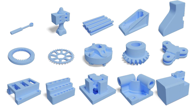
| Method | Uti. | Gap | Var. | Num. | Time |
|---|---|---|---|---|---|
| Random | 22.0% | 35.3% | 2.7 | 14.2 | 0.02 |
| Random | 23.6% | 30.6% | 2.3 | 15.2 | 0.03 |
| FF (Falkenauer 1996) | 25.0% | 26.5% | 2.5 | 16.0 | 0.03 |
| MTPE (Liu et al. 2015) | 29.3% | 13.8% | 1.9 | 18.7 | 0.03 |
| HM (Wang and Hauser 2019) | 27.4% | 19.4% | 2.0 | 17.5 | 0.03 |
| BLBF (Goyal and Deng 2020) | 28.7% | 15.6% | 1.9 | 18.3 | 0.03 |
| Ours | 34.0% | 0.0% | 1.9 | 22.6 | 0.04 |
| Ours (K = 3) | 35.3% | - | 1.7 | 23.5 | 0.06 |
| Ours (K = 5) | 37.4% | - | 1.6 | 24.5 | 0.06 |
| Ours (K = 10) | 41.0% | - | 1.7 | 25.5 | 0.06 |
B.4. Generalization across Datasets
We test generalization across datasets, that is, crossly test trained policies on other datasets. Since part of the shapes is shared between and , we conduct this experiment among , shapes from the ABC dataset, and , with 483, 136, and 8 shapes respectively. These results are summarized in Table 10. When being transferred to a new dataset, the trained policies can still show decision-making ability more competitive than heuristics.
| General | ABC | BlockOut | |||||||
|---|---|---|---|---|---|---|---|---|---|
| Train | Uti. | Var. | Num. | Uti. | Var. | Num. | Uti. | Var. | Num. |
| General | 44.5% | 3.4 | 27.7 | 33.7% | 1.7 | 22.4 | 67.5% | 1.6 | 33.2 |
| ABC | 43.3% | 4.1 | 27.2 | 34.0% | 1.9 | 22.6 | 66.1% | 1.4 | 32.4 |
| BlockOut | 38.0% | 3.7 | 24.2 | 29.7% | 1.4 | 20.0 | 71.0% | 1.7 | 34.8 |
| Random | 31.6% | 5.8 | 19.6 | 22.0% | 2.7 | 14.2 | 37.1% | 3.4 | 17.8 |
| Heuristic | 37.3% | 4.6 | 22.7 | 29.3% | 1.9 | 18.7 | 61.9% | 4.1 | 29.5 |
We note that policies trained on datasets with more variety of shapes tend to perform better on one out-of-distribution dataset. To confirm this, we train policies with different numbers of shapes from and test them on ABC and . Results are visualized in Fig. 20. We can see that rich training shapes help policies transfer to the other two datasets. We recommend that users increase shape variety to enable better performance on out-of-distribution shapes.
B.5. Product Utility
We evaluate packing results with a new product utility metric, which is defined as the initial bounding box volume of all placed items divided by the container volume:
| (6) |
where is the container volume. This metric is widely used in the manufacturing industry to reveal the connection between irregular and bin packing. We calculate this metric on all datasets and present the results in Table 11.
| Method | General | BlockOut | Kitchen | ABC |
|---|---|---|---|---|
| Random | 46.5% | 47.0% | 48.1% | 43.7% |
| Random | 48.3% | 53.4% | 54.5% | 46.8% |
| FF (Falkenauer 1996) | 53.2% | 43.0% | 59.0% | 49.6% |
| MTPE (Liu et al. 2015) | 54.8% | 58.4% | 69.3% | 58.0% |
| HM (Wang and Hauser 2019) | 52.6% | 59.5% | 70.0% | 53.9% |
| BLBF (Goyal and Deng 2020) | 53.9% | 61.9% | 68.7% | 57.2% |
| Ours | 65.1% | 90.1% | 85.4% | 67.1% |
| Ours (K = 3) | 70.4% | 90.7% | 88.3% | 68.6% |
| Ours (K = 5) | 75.6% | 94.5% | 91.7% | 70.9% |
| Ours (K = 10) | 82.7% | 98.6% | 97.4% | 73.9% |
Appendix C More Visualized Results
We provide more visualization results tested on all datasets, including industrial shapes that come from the ABC dataset. We show galleries of online PRP results on each dataset in Fig. 21. We provide qualitative results of buffered packing policies with in Fig. 22. The generalized results on buffered packing scenarios with and are visualized in Fig. 23 and Fig. 24.


