跳到论文正文
W Papers独立论文阅读器 arXiv:2212.02072 论文正文 计算阅读时间 · 0%
引用这篇论文根据当前论文元数据生成,正式投稿前建议核对。


Robust Reinforcement Learning for Risk-Sensitive Linear Quadratic Gaussian Control

Leilei Cui    Tamer Başar    Life Fellow, IEEE,    Zhong-Ping Jiang    Fellow, IEEE Thanks: *This work has been supported in part by the NSF grants EPCN-1903781 and ECCS-2210320. Thanks: L. Cui and Z.˜P.˜Jiang are with the Control and Networks Lab, Department of Electrical and Computer Engineering, Tandon School of Engineering, New York University, Brooklyn, NY 11201, USA (e-mail: l.cui@nyu.edu; zjiang@nyu.edu). Thanks: T. Başar is with the Coordinated Science Laboratory, University of Illinois Urbana-Champaign, Urbana, IL 61801 USA (e-mail: basar1@illinois.edu).
Abstract

This paper proposes a novel robust reinforcement learning framework for discrete-time linear systems with model mismatch that may arise from the sim-to-real gap. A key strategy is to invoke advanced techniques from control theory. Using the formulation of the classical risk-sensitive linear quadratic Gaussian control, a dual-loop policy optimization algorithm is proposed to generate a robust optimal controller. The dual-loop policy optimization algorithm is shown to be globally and uniformly convergent, and robust against disturbances during the learning process. This robustness property is called small-disturbance input-to-state stability and guarantees that the proposed policy optimization algorithm converges to a small neighborhood of the optimal controller as long as the disturbance at each learning step is relatively small. In addition, when the system dynamics is unknown, a novel model-free off-policy policy optimization algorithm is proposed. Finally, numerical examples are provided to illustrate the proposed algorithm.

Index Terms: 
Robust reinforcement learning, policy optimization, risk-sensitive LQG.

I Introduction

By optimizing a specified accumulated performance index, reinforcement learning (RL), as a branch of machine learning, is aimed at learning optimal decisions from data in the absence of model knowledge. Policy optimization (PO) plays a pivotal role in the development of RL algorithms [1, Chapter 13]. The key idea of PO is to parameterize the policy and update the policy parameters along the gradient ascent direction of the performance index for maximization, or gradient descent for minimization. Since the system model is unknown, the policy gradient should be estimated by data-driven methods through sampling and experimentation. Consequently, accurate policy gradient can hardly be obtained because of various errors that may be induced by function approximation, measurement noise, and external disturbance. Therefore, both convergence and robustness properties of PO should be theoretically studied in the presence of gradient estimation error.

Since linear quadratic regulator (LQR) is theoretically tractable and widely applied in various engineering fields, it stands out as providing an ideal benchmark for studying RL problems. For the LQR problem, the control policy is parameterized as a linear function of the state, i.e. ut=−K​xtu_{t}=-Kx_{t}. The corresponding performance index is 𝒥L​Q​R​(K)=∑t=0∞𝔼⁡(xtT​Q​xt+utT​R​ut)\mathcal{J}_{LQR}(K)=\sum_{t=0}^{\infty}\mathbb{E}(x_{t}^{T}Qx_{t}+u_{t}^{T}Ru_{t}). PO for the LQR problem aims at solving the constrained optimization problem minK∈𝒲⁡𝒥L​Q​R​(K)\min_{K\in\mathcal{W}}\mathcal{J}_{LQR}(K), where 𝒲\mathcal{W} is the admissible set of stabilizing control policies. Since 𝒥L​Q​R​(K)\mathcal{J}_{LQR}(K) can be expressed in terms of a Lyapunov equation, which depends on KK, 𝒥L​Q​R​(K)\mathcal{J}_{LQR}(K) is differentiable in KK. Based on this result, standard gradient descent, natural policy gradient, and Newton gradient algorithms have been developed to minimize the performance index 𝒥L​Q​R​(K)\mathcal{J}_{LQR}(K) [2, 3, 4, 5, 6, 7]. Interestingly, the Newton gradient algorithm with a step size of 12\frac{1}{2} is equivalent to the celebrated Kleinman’s policy iteration algorithm [8, 9, 10, 11]. By the coercive property of the performance index 𝒥L​Q​R​(K)\mathcal{J}_{LQR}(K) (𝒥L​Q​R​(K)→∞\mathcal{J}_{LQR}(K)\to\infty as K→∂𝒲K\to\partial\mathcal{W}), the stability of the updated control policy is maintained during PO. Furthermore, the global linear convergence rate of the algorithms is theoretically demonstrated by the gradient dominance property which is shown in [4, Remark 2] and [5, Lemma 3]. One of the reasons for using PO in these model-based approaches (perhaps the most important one) is that it provides a natural pathway to model-free analysis, where the RL techniques come into play. For example, when the system model is unknown, zeroth-order methods are applied to approximate the gradient of the performance index, supported by a sample complexity analysis [5, 7, 4]. Since the estimation error of policy gradient is inevitable at each iteration, whether the error will accumulate and whether the adopted algorithms still converge in the presence of estimation error should be further studied. By considering the PO algorithm as a nonlinear discrete-time system and invoking input-to-state stability [12], the authors of [13, 14] show that the Kleinman’s policy iteration algorithm can still find a near-optimal control policy even under the influence of estimation error. A similar robustness property is investigated for the steepest gradient descent algorithm [15].

The aforementioned PO for the LQR problem cannot guarantee the robustness of the closed-loop system. For example, the obtained controller may fail to stabilize the system in the presence of model mismatch that may be induced by the sim-to-real gap and parameter variation. Risk-sensitive linear quadratic Gaussian (LQG) control was first proposed by [16, 17], which generalizes the risk-neutral optimal control (i.e. LQR) by minimizing the expectation of the accumulative quadratic cost transformed by the exponential function. It was shown in [18] and [19] that the risk-sensitive LQG control is equivalent to the mixed ℋ2\mathcal{H}_{2}/ℋ∞\mathcal{H}_{\infty} control and the linear quadratic zero-sum dynamic game. Therefore, it can guarantee the stability of the closed-loop system even under model mismatch. The authors of [20, 21, 22] proposed RL algorithms for solving the model-free risk-sensitive control, but the methods are only applicable to Markov decision processes whose state and action spaces are finite. In [23, 24], the authors proposed Q-learning algorithms for linear quadratic zero-sum dynamic games. The paper [25] proposed PO methods for mixed ℋ2/ℋ∞\mathcal{H}_{2}/\mathcal{H}_{\infty} control to guarantee robust stability of the closed-loop system. Through the concept of implicit regularization, it was shown that the proposed PO algorithms can find the globally optimal solution of mixed ℋ2/ℋ∞\mathcal{H}_{2}/\mathcal{H}_{\infty} control at globally sublinear and locally superlinear rates. As there is a fundamental connection between mixed ℋ2/ℋ∞\mathcal{H}_{2}/\mathcal{H}_{\infty} control and linear-quadratic zero-sum dynamic games (LQ ZSDGs), the natural policy gradient and Newton algorithms have been equivalently transformed into provably convergent dual-loop PO algorithms for the LQ ZSDG [26, 27, 28]. The outer loop is to learn a protagonist under the worst-case adversary while the inner loop is to learn a worst-case adversary. In this way, the protagonist can robustly perform the control tasks under the disturbances created by the adversary. Interestingly, the Newton algorithm with a step size of 12\frac{1}{2} is equivalent to the policy iteration algorithm for ZSDG [29, 30, 31]. In the aforementioned papers, the convergence of the learning algorithms for the risk-sensitive control has been analyzed under the ideal noise-free case. Besides the convergence, a useful learning algorithm should be robust and is capable of finding a near-optimal solution even in the face of noise that may be induced by noisy experimental data, rounding errors of numerical computation, or the finite-time stopping of the inner loop in the dual-loop learning setup. However, the issues of uniform convergence and robustness of the dual-loop learning algorithm are still unsolved.

I-A Our Contributions in this Paper

A fundamental challenge of the convergence of the dual-loop PO algorithm is to address the uniform convergence issue tied to the inner loop. Specifically, the required number of inner-loop iterations should be independent of the outer-loop iteration. Otherwise, as the outer-loop iteration increases, the required number of inner-loop iterations may grow explosively, thus making the dual-loop algorithm not practically implementable. To the best of our knowledge, the uniform convergence of the dual-loop algorithm has not been theoretically analyzed heretofore.

In addition, PO algorithm cannot be implemented accurately in practical applications, due to the influence of various errors arising from gradient estimation error, sensor noise, external disturbance, and modeling error. Hence, a fundamental question arises: Is the PO algorithm robust to the errors? In particular, does the PO algorithm still converge to a neighbourhood of the optimal solution in the presence of various errors and, if yes, what is the size of the neighborhood? For both the outer and inner loops, the iterative process is nonlinear, and the robustness of the PO algorithm has not been fully understood in the present literature.

In this paper, we investigate uniform convergence and robustness of the dual-loop iterative algorithm for solving the problem of risk-sensitive linear quadratic Gaussian control. Even though the convergence of the dual-loop iterative algorithm is analyzed separately in [25, 28, 5], uniform convergence and robustness of the overall algorithm are still open problems. To analyze the uniform convergence of the dual-loop algorithm, the key idea is to demonstrate global linear convergence of the inner-loop iteration and find an upperbound on the linear convergence rate. To address the robustness issue, a key strategy of the paper is to invoke techniques from advanced control theory, such as input-to-state stability (ISS) [12] and its latest variant called “small-disturbance ISS” [13] to analyze the robustness of the proposed discrete-time iterative algorithm. In the presence of noise during the learning process, it is demonstrated that the PO algorithm still converges to a small neighbourhood of the optimal solution, as long as the noise is relatively small. Furthermore, based on these results and the technique of approximate dynamic programming [32, 33], an off-policy data-driven RL algorithm is proposed when the system is disturbed by an immeasurable Gaussian noise. Several numerical examples are given to validate the efficacy of our theoretical results.

To sum up, our main contributions in this paper are three-fold: 1) the uniform convergence of the dual-loop iterative algorithm is theoretically analyzed; 2) under the framework of the small-disturbance ISS, the robustness of both the outer and inner loops is theoretically demonstrated; 3) a novel learning-based off-policy policy optimization algorithm is proposed.

A shorter and preliminary version of this paper was presented at the conference L4DC 2023 [34]. Compared with the conference paper, in this paper, we provide rigorous proofs for all the theoretical results. In addition, in Section V-A, we propose a method to learn an initial admissible controller. Finally, a benchmark example known as cart-pole system is provided to demonstrate the effectiveness of the proposed dual-loop algorithm.

I-B Organization of the Paper

Following this Introduction section, Section II provides some preliminaries on linear exponential quadratic Gaussian (LEQG) control problem, LQG zero-sum dynamic game, and robustness analysis. Section III introduces the model-based dual-loop iterative algorithm to optimize the policy for LEQG control, and the convergence of the algorithm is analyzed. Section IV analyzes robustness of the dual-loop iterative algorithm to various errors in the learning process within the framework of ISS. Section V presents a learning-based policy optimization algorithm for LEQG control. Section VI provides two numerical examples to illustrate the proposed algorithm. The paper ends with the concluding remarks of Section VII and six appendices which include proofs of the main results in the main body of the paper.

I-C Notations

ℝ\mathbb{R} and ℂ\mathbb{C} are the sets of real and complex numbers, respectively. ℤ\mathbb{Z} (ℤ+\mathbb{Z}_{+}) is the set of (positive) integers. 𝕊n\mathbb{S}^{n} is the set of nn-dimensional real symmetric matrices. |a||a| denotes the Euclidean norm of a vector aa. ∥⋅∥\lVert\cdot\rVert and ∥⋅∥F\lVert\cdot\rVert_{F} denote the spectral norm and the Frobenius norm of a matrix. ℓ2\ell_{2} is the space of square-summable sequences equipped with the norm ∥⋅∥2\lVert\cdot\rVert_{2}. ℓ∞\ell_{\infty} is the space of bounded sequences equipped with the norm ∥⋅∥∞\lVert\cdot\rVert_{\infty}. σ¯(⋅)\bar{\sigma}(\cdot) and σ¯(⋅)\underline{\sigma}(\cdot) are respectively the maximum and minimum singular values of a given matrix. For a transfer function G⁡(z)G(z), its ℋ∞\mathcal{H}_{\infty} norm is defined as ∥G∥ℋ∞:=supω∈[0,2​π]σ¯​(G⁡(ej​ω))\lVert G\rVert_{\mathcal{H}_{\infty}}:=\sup_{\omega\in[0,2\pi]}\bar{\sigma}(G(e^{j\omega})), which is equivalent to ∥G∥ℋ∞:=supu∈ℓ2∥G​u∥2∥u∥2\lVert G\rVert_{\mathcal{H}_{\infty}}:=\sup_{u\in\ell_{2}}\frac{\lVert Gu\rVert_{2}}{\lVert u\rVert_{{}_{2}}}.

For a matrix X∈ℝm×nX\in\mathbb{R}^{m\times n}, vec⁡(X):=[x1T,⋯,xnT]T\vect(X):=[x_{1}^{T},\cdots,x_{n}^{T}]^{T}, where xix_{i} is the iith column of XX. For a matrix P∈𝕊nP\in\mathbb{S}^{n}, vecs⁡(P):=[p1,1,p1,2,⋯,p1,n,p2,2,p2,3,⋯,pn,n]T\vecs(P):=[p_{1,1},p_{1,2},\cdots,p_{1,n},p_{2,2},p_{2,3},\cdots,p_{n,n}]^{T}, where pi,jp_{i,j} is the iith row and jjth column entry of the matrix PP. [X]i[X]_{i} dentotes the iith row of XX. [X]i,j[X]_{i,j} denotes the submatrix of the matrix XX that is comprised of the rows between the iith and jjth rows of XX. For a vector a∈ℝna\in\mathbb{R}^{n}, vecv⁡(a):=[a12,2​a1​a2,⋯,2​a1​an,a22,2​a2​a3,⋯,an2]T\vecv(a):=[a_{1}^{2},2a_{1}a_{2},\cdots,2a_{1}a_{n},a_{2}^{2},2a_{2}a_{3},\cdots,a_{n}^{2}]^{T}. InI_{n} denotes the nn-dimensional identity matrix.

II Preliminaries

In this section, we begin with the problem formulation of LEQG control. Then, we discuss its relation to linear quadratic zero-sum dynamic games (DG) and its robustness analysis.

II-A Linear Exponential Quadratic Guassian Control

Consider the discrete-time linear time-invariant system

xt+1\displaystyle x_{t+1} =A​xt+B​ut+D​wtx0∼𝒩⁡(0,In),\displaystyle=Ax_{t}+Bu_{t}+Dw_{t}\quad x_{0}\sim\mathcal{N}(0,I_{n}), (1a)
yt\displaystyle y_{t} =C​xt+E​ut,\displaystyle=Cx_{t}+Eu_{t}, (1b)

where xt∈ℝnx_{t}\in\mathbb{R}^{n} is the state of the system; ut∈ℝmu_{t}\in\mathbb{R}^{m} is the control input; x0x_{0} is the initial state; wt∈ℝq∼𝒩⁡(0,Iq)w_{t}\in\mathbb{R}^{q}\sim\mathcal{N}(0,I_{q}) is independent and identically distributed random variable; yt∈ℝpy_{t}\in\mathbb{R}^{p} is the controlled output. A,B,C,D,EA,\,B,\,C,\,D,\,E are constant matrices with compatible dimensions. The LEQG control problem entails finding an input sequence u:={ut}t=0∞u:=\{u_{t}\}_{t=0}^{\infty}, depending on the current value of the state, that is {ut=μt(xt)}t=0∞\{u_{t}=\mu_{t}(x_{t})\}^{\infty}_{t=0} where μ:={μt:ℝn→ℝm}t=0∞\mu:=\{\mu_{t}:\mathbb{R}^{n}\to\mathbb{R}^{m}\}^{\infty}_{t=0} is a seqence of appropriately defined measurable control policies, such that the following risk-averse exponential quadratic cost is minimized

𝒥L​E​Q​G​(μ):=limτ→∞2​γ2τ​log⁡[𝔼​exp⁡(12​γ2​∑t=0τytT​yt)]\displaystyle\mathcal{J}_{LEQG}(\mu):=\lim_{\tau\to\infty}\frac{2\gamma^{2}}{\tau}\log\left[\mathbb{E}\exp\left(\frac{1}{2\gamma^{2}}\sum_{t=0}^{\tau}y^{T}_{t}y_{t}\right)\right] (2)

where γ\gamma is a positive constant. For proper formulation of the optimization problem, the following two assumptions are standard.

Assumption 1.

(A,B)(A,B) is stabilizable, CT​C=Q≻0C^{T}C=Q\succ 0, and γ>γ∞\gamma>\gamma_{\infty}, where γ∞>0\gamma_{\infty}>0 is the minimal value of γ\gamma such that for γ>γ∞\gamma>\gamma_{\infty} the solution to (6) given below exists, or equivalently there exists a control under which (2) is finite.

Assumption 2.

The matrices in (1b) satisfy ET​E=R≻0E^{T}E=R\succ 0, and CT​E=0C^{T}E=0.

Assumption 1 ensures the existence of a stabilizing solution to the LEQG control problem. As demonstrated in [19, Theorem 3.8], γ∞\gamma_{\infty} is finite. In addition, the positive definiteness of Q≻0Q\succ 0 can be relaxed to Q⪰0Q\succeq 0, as long as (A,C)(A,C) is taken to be detectable. Assumption 2 has two parts. The first, positive definiteness of the weighting matrix on control, is standard even in LQR. The second one is also a standard condition to simplify the LEQG control problem by eliminating the cross term in the cost (2) between the control input uu and state xx. Stabilizability of the pair (A,B)(A,B) implies that there exists a feedback gain K∈ℝm×nK\in\mathbb{R}^{m\times n} such that the spectral radius ρ⁡(A−B​K)<1\rho(A-BK)<1. Henceforth, a matrix is stable if its spectral radius is less than 11, and KK is stabilizing if A−B​KA-BK is stable. A feedback gain KK is called admissible if it belongs to the admissible set 𝒲\mathcal{W} defined in (11). Assumptions 1 and 2 are used throughout the paper.

As investigated by [16] and [35, Lemma 2.1], for any admissible linear control policy μt​(xt)=−K​xt\mu_{t}(x_{t})=-Kx_{t}, the cost admits the closed-form:

𝒥L​E​Q​G(K)=−γ2logdet(In−γ−2PKDDT),\displaystyle\mathcal{J}_{LEQG}(K)=-\gamma^{2}\log\det(I_{n}-\gamma^{-2}P_{K}DD^{T}), (3)

where the matrix PK=PKT≻0P_{K}=P_{K}^{T}\succ 0 is the unique solution to

(A−B​K)T​UK​(A−B​K)−PK+Q+KT​R​K=0,\displaystyle(A-BK)^{T}U_{K}(A-BK)-P_{K}+Q+K^{T}RK=0, (4a)
UK:=PK+PK​D​(γ2​Iq−DT​PK​D)−1​DT​PK.\displaystyle U_{K}:=P_{K}+P_{K}D(\gamma^{2}I_{q}-D^{T}P_{K}D)^{-1}D^{T}P_{K}. (4b)

Furthermore, the LEQG problem admits a unique optimal controller ut∗=−K∗​xtu_{t}^{*}=-K^{*}x_{t}, where

K∗=(R+BT​U∗​B)−1​BT​U∗​A.\displaystyle K^{*}=(R+B^{T}U^{*}B)^{-1}B^{T}U^{*}A. (5)

with P∗=(P∗)T≻0P^{*}=(P^{*})^{T}\succ 0 the unique solution to the generalized algebraic Riccati equation (GARE)

(A−B​K∗)T​U∗​(A−B​K∗)−P∗+Q+(K∗)T​R​K∗=0,\displaystyle(A-BK^{*})^{T}U^{*}(A-BK^{*})-P^{*}+Q+(K^{*})^{T}RK^{*}=0, (6a)
U∗=P∗+P∗​D​(γ2​Iq−DT​P∗​D)−1​DT​P∗.\displaystyle U^{*}=P^{*}+P^{*}D(\gamma^{2}I_{q}-D^{T}P^{*}D)^{-1}D^{T}P^{*}. (6b)

II-B Linear Quadratic Zero-Sum Dynamic Game

The dynamic game can be mathematically formulated as

minμ⁡maxν​𝒥D​G​(μ,ν):=𝔼x0​(∑t=0∞ytT​yt−γ2​wtT​wt),\displaystyle\min_{\mu}\max_{\nu}\mathcal{J}_{DG}(\mu,\nu):=\mathbb{E}_{x_{0}}\left(\sum_{t=0}^{\infty}y_{t}^{T}y_{t}-\gamma^{2}w_{t}^{T}w_{t}\right),
subject to​(1),\displaystyle\text{subject to}\,\,\eqref{eq:LTI}, (7)

where u:={ut}t=0∞u:=\{u_{t}\}_{t=0}^{\infty} and w:={wt}t=0∞w:=\{w_{t}\}_{t=0}^{\infty} are the input sequences for the minimizer and the maximizer, respectively, generated by state-feedback policies μ:={μt}t=0∞\mu:=\{\mu_{t}\}^{\infty}_{t=0} and ν:={νt}t=0∞\nu:=\{\nu_{t}\}^{\infty}_{t=0}. Note that here in (1a), ww is no longer a Gaussian random sequence, but a second control variable, at the disposal of the maximizer.

For any admissible controller μt​(xt)=−K​xt\mu_{t}(x_{t})=-Kx_{t}, and with γ>γ∞\gamma>\gamma_{\infty}, the closed-form cost is

𝒥D​G​(K,ν∗​(K))=maxν⁡𝒥D​G​(−K​xt,ν)=Tr⁡(PK),\displaystyle\mathcal{J}_{DG}(K,\nu^{*}(K))=\max_{\nu}\mathcal{J}_{DG}(-Kx_{t},\nu)=\Tr(P_{K}), (8)

where PKP_{K} is the solution of (4). From [19, Equation 3.51], it follows that the optimizers for the minimax problem are μt∗​(xt)=−K∗​xt\mu_{t}^{*}(x_{t})=-K^{*}x_{t} and νt∗​(xt)=L∗​xt\nu_{t}^{*}(x_{t})=L^{*}x_{t}, where K∗K^{*} is defined in (5) and L∗L^{*} is given by

L∗=(γ2​Iq−DT​P∗​D)−1​DT​P∗​(A−B​K∗).\displaystyle L^{*}=(\gamma^{2}I_{q}-D^{T}P^{*}D)^{-1}D^{T}P^{*}(A-BK^{*}). (9)

Furthermore, (A−B​K∗)(A-BK^{*}) is stable, Iq−γ−2​DT​P∗​D≻0I_{q}-\gamma^{-2}D^{T}P^{*}D\succ 0, and (A−B​K∗+D​L∗)(A-BK^{*}+DL^{*}) is stable.

Therefore, the minimizer of DG shares the same optimal controller as the optimizer in the LEQG problem. Also note that, PKP_{K} is critical for determining the closed-from costs of 𝒥L​E​Q​G​(K)\mathcal{J}_{LEQG}(K) and 𝒥D​G​(K,ν∗)\mathcal{J}_{DG}(K,\nu^{*}).

II-C Robustness Analysis

With ww taken as a deterministic input in (1), and taking any stabilizing feedback μt​(xt)=−K​xt\mu_{t}(x_{t})=-Kx_{t}, the discrete-time transfer function from ww to yy can be expressed as

𝒯⁡(K):=(C−E​K)​[z​In−(A−B​K)]−1​D.\displaystyle\mathcal{T}(K):=(C-EK)[zI_{n}-(A-BK)]^{-1}D. (10)

where z∈ℂz\in\mathbb{C} is the zz-transform variable.

Now consider the depiction in Fig. 1, where Δ\Delta denotes the model mismatch that may be induced by the sim-to-real gap, and satisfying ∥Δ∥ℋ∞≤1γ\lVert\Delta\rVert_{\mathcal{H}_{\infty}}\leq\frac{1}{\gamma}. Thanks to the small-gain theorem [36, 37, 38], when subjected to model mismatch, the system remains stable as long as ∥𝒯⁡(K)∥ℋ∞<γ\lVert\mathcal{T}(K)\rVert_{\mathcal{H}_{\infty}}<\gamma. Consequently, the controller μt​(xt)=−K​xt\mu_{t}(x_{t})=-Kx_{t} is robust to the model mismatch Δ\Delta if KK lies within the admissible set 𝒲\mathcal{W} defined as

𝒲:={K∈ℝm×n|ρ(A−BK)<1,∥𝒯(K)∥ℋ∞<γ}.\displaystyle\mathcal{W}:=\{K\in\mathbb{R}^{m\times n}|\rho(A-BK)<1,\lVert\mathcal{T}(K)\rVert_{\mathcal{H}_{\infty}}<\gamma\}. (11)

As investigated in [19, Theorem 3.8], the LEQG control in (5) satisfies K∗∈𝒲K^{*}\in\mathcal{W}, and therefore, it is optimal with respect to (2) and robust to the model mismatch. This motivates us to pose the following problem.

Problem 1.

Design a learning-based control algorithm such that near-optimal control gains, i.e. approximate values of K∗K^{*}, can be learned from the input-state data.

We will first introduce the model-based PO algorithm whose convergence and robustness properties are instrumental for the learning-based algorithm.

Refer to caption
Fig. 1: Robust control design with model mismatch Δ\Delta.

III Model-based Policy Optimization

In this section, by resorting to the PO method, a dual-loop iterative algorithm is proposed.

III-A Introduction of the Outer Loop

The outer-loop iteration is developed based on the Newton PO algorithm in [35]. For any K∈𝒲K\in\mathcal{W}, the gradient ∇K𝒥​(K)=∇K𝒥L​E​Q​G​(K)=∇K𝒥D​G​(K,ν∗​(K))\nabla_{K}\mathcal{J}(K)=\nabla_{K}\mathcal{J}_{LEQG}(K)=\nabla_{K}\mathcal{J}_{DG}(K,\nu^{*}(K)) can be computed to be

∇K𝒥​(K)=2​[(R+BT​UK​B)​K−BT​UK​A]​ΣK,\displaystyle\begin{split}&\nabla_{K}\mathcal{J}(K)=2[(R+B^{T}U_{K}B)K-B^{T}U_{K}A]\Sigma_{K},\end{split} (12)

where

ΣK\displaystyle\Sigma_{K} =∑t=0∞[(A−B​K+D​LK,∗)T]t​D\displaystyle=\sum_{t=0}^{\infty}[(A-BK+DL_{K,*})^{T}]^{t}D (13)
(Iq−γ−2​DT​PK​D)−1​DT​(A−B​K+D​LK,∗)t.\displaystyle(I_{q}-\gamma^{-2}D^{T}P_{K}D)^{-1}D^{T}(A-BK+DL_{K,*})^{t}.

and

LK,∗:=(γ2​Iq−DT​PK​D)−1​DT​PK​(A−B​K),\displaystyle L_{K,*}:=(\gamma^{2}I_{q}-D^{T}P_{K}D)^{-1}D^{T}P_{K}(A-BK), (14)

It is noticed that given ut=−K​xtu_{t}=-Kx_{t}, LK,∗L_{K,*} is considered as a worst-case feedback gain for ww. 11 1 Henceforth, we write μt​(xt)=−K​xt\mu_{t}(x_{t})=-Kx_{t} simply as ut=−K​xtu_{t}=-Kx_{t}, and likewise for ww, as appropriate. By the Newton method with a step size of 12\frac{1}{2}, to iteratively minimize 𝒥⁡(K)\mathcal{J}(K), the updated feedback gain is

K′=K−12​(R+BT​UK​B)−1​∇K𝒥​(K)​ΣK−1=(R+BT​UK​B)−1​BT​UK​A.\displaystyle\begin{split}K^{\prime}&=K-\frac{1}{2}(R+B^{T}U_{K}B)^{-1}\nabla_{K}\mathcal{J}(K)\Sigma_{K}^{-1}\\ &=(R+B^{T}U_{K}B)^{-1}B^{T}U_{K}A.\end{split} (15)

Let ii denote the iteration index for the outer loop and introduce the following variables to simplify the notation

Ai:=A−B​Ki,Qi:=Q+KiT​R​Ki,\displaystyle A_{i}:=A-BK_{i},\quad Q_{i}:=Q+K_{i}^{T}RK_{i}, (16a)

where AiA_{i} is the closed-loop transition matrix with ut=−Ki​xtu_{t}=-K_{i}x_{t}, and QiQ_{i} is the cost weighting matrix. Then, by (4) and (15), the outer-loop iteration can be expressed as

AiT​Ui​Ai−Pi+Qi=0,\displaystyle A_{i}^{T}U_{i}A_{i}-P_{i}+Q_{i}=0, (17a)
Ui:=Pi+Pi​D​(γ2​Iq−DT​Pi​D)−1​DT​Pi,\displaystyle U_{i}:=P_{i}+P_{i}D(\gamma^{2}I_{q}-D^{T}P_{i}D)^{-1}D^{T}P_{i}, (17b)
Ki+1=(R+BT​Ui​B)−1​BT​Ui​A,\displaystyle K_{i+1}=(R+B^{T}U_{i}B)^{-1}B^{T}U_{i}A, (17c)

In (17), from policy iteration perspective [33], we consider (17a) as the policy evaluation step under the worst-case disturbance and (17c) as the policy improvement step. PiP_{i} is the cost matrix of (II-B) for the controller ut=−Ki​xtu_{t}=-K_{i}x_{t} under the worst-case disturbance.

As seen in Lemma 5, for each iteration, the controller KiK_{i} generated by (17) preserves robustness to model mismatch, i.e. Ki∈𝒲K_{i}\in\mathcal{W}. PiP_{i} converges to P∗P^{*} with a globally sublinear and locally quadratic rate [25, Theorems 4.3 and 4.4]. We further investigate the convergence rate of (17) and rigorously demonstrate that PiP_{i} monotonically converges to the optimal solution P∗P^{*} with a globally linear convergence rate. The proof of the following theorem can be found in Appendix B.

Theorem 1.

Let ℋ:={Tr⁡(PK)−Tr⁡(P∗)|K∈𝒲}\mathcal{H}:=\{\Tr(P_{K})-\Tr(P^{*})|K\in\mathcal{W}\}. For any h∈ℋh\in\mathcal{H} and K1∈𝒢hK_{1}\in\mathcal{G}_{h}, where 𝒢h={K∈𝒲|Tr⁡(PK)≤Tr⁡(P∗)+h}\mathcal{G}_{h}=\{K\in\mathcal{W}|\Tr(P_{K})\leq\Tr(P^{*})+h\}, there exists α⁡(h)∈[0,1)\alpha(h)\in[0,1), such that

Tr⁡(Pi+1−P∗)≤α⁡(h)​Tr⁡(Pi−P∗),∀i∈ℤ+.\displaystyle\Tr(P_{i+1}-P^{*})\leq\alpha(h)\Tr(P_{i}-P^{*}),\quad\forall i\in\mathbb{Z}_{+}. (18)

Since Pi+1−P∗⪰0P_{i+1}-P^{*}\succeq 0 and ∥Pi+1−P∗∥F≤Tr⁡(Pi+1−P∗)≤n​∥Pi+1−P∗∥F\lVert P_{i+1}-P^{*}\rVert_{F}\leq\Tr(P_{i+1}-P^{*})\leq\sqrt{n}\lVert P_{i+1}-P^{*}\rVert_{F} (Lemma 3), the following inequlity holds

∥Pi+1−P∗∥F≤n​αi​(h)​∥P1−P∗∥F.\displaystyle\lVert P_{i+1}-P^{*}\rVert_{F}\leq\sqrt{n}\alpha^{i}(h)\lVert P_{1}-P^{*}\rVert_{F}. (19)

Since 𝒥D​G​(Ki,ν∗​(Ki))=Tr⁡(Pi)\mathcal{J}_{DG}(K_{i},\nu^{*}(K_{i}))=\Tr(P_{i}) from (8), it follows that

𝒥D​G​(Ki+1,ν∗​(Ki+1))−𝒥D​G​(μ∗,ν∗)≤α⁡(h)​[𝒥D​G​(Ki,ν∗​(Ki))−𝒥D​G​(μ∗,ν∗)].\displaystyle\begin{split}&\mathcal{J}_{DG}(K_{i+1},\nu^{*}(K_{i+1}))-\mathcal{J}_{DG}(\mu^{*},\nu^{*})\leq\\ &\alpha(h)[\mathcal{J}_{DG}(K_{i},\nu^{*}(K_{i}))-\mathcal{J}_{DG}(\mu^{*},\nu^{*})].\end{split} (20)

Hence, the cost of the dynamic game (under the worst-case disturbance) converges to the saddle point at a linear convergence rate α⁡(h)∈[0,1)\alpha(h)\in[0,1).

In the following subsection, given KiK_{i}, by maximizing 𝒥D​G​(Ki,ν)\mathcal{J}_{DG}(K_{i},\nu) over ν\nu, the inner-loop iteration is developed to get the worst-case disturbance ν∗​(Ki)\nu^{*}(K_{i}).

III-B Introduction of the Inner Loop

Given the feedback gain of the minimizer K∈𝒲K\in\mathcal{W}, the inner loop iteratively finds the optimal controller for the maximizer w∗​(K)w^{*}(K) by solving 22 2 Here and below, we have used the control ww instead of the policy ν\nu, for simplicity of the notation.

maxw⁡𝒥D​G​(K,w)=∑t=0∞ytT​yt−γ2​wtT​wt,\displaystyle\max_{w}\mathcal{J}_{DG}(K,w)=\sum_{t=0}^{\infty}y_{t}^{T}y_{t}-\gamma^{2}w_{t}^{T}w_{t}, (21)
subject to​xt+1=(A−B​K)​xt+D​wt,x0∼𝒩⁡(0,In).\displaystyle\text{subject to}\,\,x_{t+1}=(A-BK)x_{t}+Dw_{t},x_{0}\sim\mathcal{N}(0,I_{n}).

The optimal solution is wt∗​(K)=LK,∗​xtw^{*}_{t}(K)=L_{K,*}x_{t}, where LK,∗L_{K,*} is defined in (14). For any admissible controller wt=L​xtw_{t}=Lx_{t} (with (A−B​K+D​LA-BK+DL) stable), by [5] the closed-form cost is

𝒥D​G​(K,L)=Tr⁡(PK,L),\displaystyle\mathcal{J}_{DG}(K,L)=\Tr(P_{K,L}), (22)

where PK,L=PK,LT≻0P_{K,L}=P_{K,L}^{T}\succ 0 is the solution to

(A−B​K+D​L)T​PK,L​(A−B​K+D​L)−PK,L+Q+KT​R​K−γ2​LT​L=0\displaystyle\begin{split}&(A-BK+DL)^{T}P_{K,L}(A-BK+DL)\\ &-P_{K,L}+Q+K^{T}RK-\gamma^{2}L^{T}L=0\end{split} (23)

The gradient of ∇L𝒥D​G​(K,L)\nabla_{L}\mathcal{J}_{DG}(K,L) is

∇L𝒥D​G(K,L)=2[(γ2Iq−DTPK,LD)L−DTPK,L(A−BK)]ΣK,L,\displaystyle\begin{split}&\nabla_{L}\mathcal{J}_{DG}(K,L)=2\left[(\gamma^{2}I_{q}-D^{T}P_{K,L}D)L\right.\\ &\left.-D^{T}P_{K,L}(A-BK)\right]\Sigma_{K,L},\end{split} (24)

where

ΣK,L\displaystyle\Sigma_{K,L} =∑t=0∞(A−B​K+D​L)t​[(A−B​K+D​L)T]t.\displaystyle=\sum_{t=0}^{\infty}(A-BK+DL)^{t}[(A-BK+DL)^{T}]^{t}. (25)

By Newton methods, the updated feedback gain is

L′\displaystyle L^{\prime} =L−12(γ2Iq−DTPK,LD)−1∇𝒥D​G(K,L)ΣK,L−1\displaystyle=L-\frac{1}{2}(\gamma^{2}I_{q}-D^{T}P_{K,L}D)^{-1}\nabla\mathcal{J}_{DG}(K,L)\Sigma_{K,L}^{-1}
=(γ2​Iq−DT​PK,L​D)−1​DT​PK,L​(A−B​K).\displaystyle=(\gamma^{2}I_{q}-D^{T}P_{K,L}D)^{-1}D^{T}P_{K,L}(A-BK). (26)

Let jj denote the iteration index of the inner loop, and introduce the following variables to simplify the notation:

Ai,j\displaystyle A_{i,j} :=A−B​Ki+D​Li,j,Qi:=Q+KiT​R​Ki,\displaystyle:=A-BK_{i}+DL_{i,j},Q_{i}:=Q+K_{i}^{T}RK_{i}, (27a)
Ai,∗\displaystyle A_{i,*} :=A−B​Ki+D​Li,∗,A∗:=A−B​K∗+D​L∗.\displaystyle:=A-BK_{i}+DL_{i,*},A^{*}:=A-BK^{*}+DL^{*}. (27b)

By (23) and (III-B), the inner loop is designed as

Ai,jT​Pi,j​Ai,j−Pi,j+Qi−γ2​Li,jT​Li,j=0,\displaystyle A_{i,j}^{T}P_{i,j}A_{i,j}-P_{i,j}+Q_{i}-\gamma^{2}L_{i,j}^{T}L_{i,j}=0, (28a)
Li,j+1=(γ2​Iq−DT​Pi,j​D)−1​DT​Pi,j​Ai.\displaystyle L_{i,j+1}=(\gamma^{2}I_{q}-D^{T}P_{i,j}D)^{-1}D^{T}P_{i,j}A_{i}. (28b)

From the policy iteration perspective, we consider (28a) as the policy evaluation step and (28b) as the policy improvement step for the inner loop. Pi,jP_{i,j} is the cost matrix of 𝒥D​G​(Ki,Li,j)\mathcal{J}_{DG}(K_{i},L_{i,j}) with the state-feedback policies μt​(xt)=−Ki​xt\mu_{t}(x_{t})=-K_{i}x_{t} and νt​(xt)=Li,j​xt\nu_{t}(x_{t})=L_{i,j}x_{t}. The inner-loop policy iteration possesses the monotonicity property and preserves stability, that is the sequence {Pi,j}j=1∞\{P_{i,j}\}_{j=1}^{\infty} is monotonically increasing and upper bounded by PiP_{i}, and A−B​Ki+D​Li,jA-BK_{i}+DL_{i,j} is stable. These results are stated in Lemma 12. We prove that the inner loop globally and linearly converges to the optimal solution PiP_{i}. The details of the proof are given in Appendix C. This brings us to the following theorem, whose proof is in Appendix C.

Theorem 2.

Given Li,1=0L_{i,1}=0, for any Ki∈𝒲K_{i}\in\mathcal{W}, there exists a constant β⁡(Ki)∈[0,1)\beta(K_{i})\in[0,1), such that

Tr⁡(Pi−Pi,j+1)≤β⁡(Ki)​Tr⁡(Pi−Pi,j),∀j∈ℤ+.\displaystyle\Tr(P_{i}-P_{i,j+1})\leq\beta(K_{i})\Tr(P_{i}-P_{i,j}),\quad\forall j\in\mathbb{Z}_{+}. (29)

Based on Theorem 2, we can further obtain that

∥Pi−Pi,j+1∥F≤n​βj​(Ki)​∥Pi−Pi,1∥F.\displaystyle\lVert P_{i}-P_{i,j+1}\rVert_{F}\leq\sqrt{n}\beta^{j}(K_{i})\lVert P_{i}-P_{i,1}\rVert_{F}. (30)

In addition, since 𝒥D​G​(Ki,Li,j)=Tr⁡(Pi,j)\mathcal{J}_{DG}(K_{i},L_{i,j})=\Tr(P_{i,j}) and 𝒥D​G​(Ki,Li,∗)=Tr⁡(Pi)\mathcal{J}_{DG}(K_{i},L_{i,*})=\Tr(P_{i}), from Theorem 2, we have

𝒥D​G​(Ki,Li,∗)−𝒥D​G​(Ki,Li,j+1)≤β⁡(Ki)​[𝒥D​G​(Ki,Li,∗)−𝒥D​G​(Ki,Li,j)].\displaystyle\begin{split}&\mathcal{J}_{DG}(K_{i},L_{i,*})-\mathcal{J}_{DG}(K_{i},L_{i,j+1})\leq\\ &\beta(K_{i})[\mathcal{J}_{DG}(K_{i},L_{i,*})-\mathcal{J}_{DG}(K_{i},L_{i,j})].\end{split} (31)

Hence, the cost of the dynamic game with KiK_{i} is monotonically increasing and converges to the maximum at a linear rate β⁡(Ki)∈[0,1)\beta(K_{i})\in[0,1).

The dual-loop policy iteration algorithm is in Algorithm 1. Ideally, Pi,jP_{i,j} generated by the inner loop converges to PiP_{i}, and then the control gain for the minimizer is updated to Ki+1K_{i+1} by (17c). In practice, the inner loop stops after j¯\bar{j} iterations, and Pi,j¯P_{i,\bar{j}}, instead of PiP_{i}, is used for updating the control gain at line 12. Ki,j¯K_{i,\bar{j}} denotes the control gain updated at the outer loop.

III-C Convergence Analysis for the Dual-Loop Algorithm

For the dual-loop algorithm, the inner-loop iteration linearly converges to the optimal solution PKP_{K} with the rate dependent on KK. Since KK is updated iteratively, it is required that the inner loop enter the given neighborhood of PKP_{K} within a constant number of steps, regardless of KK. Otherwise, as the outer-loop iteration proceeds, the required number of inner-loop iterations may grow explosively, thus making the dual-loop algorithm not practically implementable. The uniform convergence rate of the overall algorithm is given in the following theorem, whose proof is given in Appendix D.

Theorem 3.

For any h∈ℋh\in\mathcal{H}, K∈𝒢hK\in\mathcal{G}_{h}, and ϵ>0\epsilon>0, there exists j¯​(h,ϵ)∈ℤ+\bar{j}(h,\epsilon)\in\mathbb{Z}_{+} independent of KK, such that for all j≥j¯​(h,ϵ)j\geq\bar{j}(h,\epsilon), ∥PK,j−PK∥F≤ϵ\lVert P_{K,j}-P_{K}\rVert_{F}\leq\epsilon.

Algorithm 1 Model-Based Policy Optimization
1: Set i¯,j¯∈ℤ+\bar{i},\bar{j}\in\mathbb{Z}_{+}. Initialize K1,j¯∈𝒲K_{1,\bar{j}}\in\mathcal{W}  
2: for i≤i¯i\leq\bar{i} do
3:   Initialize j=1j=1 and Li,1=0L_{i,1}=0 
4:   Qi,j¯=CT​C+Ki,j¯T​R​Ki,j¯Q_{i,\bar{j}}=C^{T}C+K_{i,\bar{j}}^{T}RK_{i,\bar{j}} 
5:   for j≤j¯j\leq\bar{j} do
6:    Ai,j=A−B​Ki,j¯+D​Li,jA_{i,j}=A-BK_{i,\bar{j}}+DL_{i,j} 
7:    Get Pi,jP_{i,j} by solving (28a) 
8:    Update Li,j+1L_{i,j+1} by (28b) 
9:    j←j+1j\leftarrow j+1  
10:   end for
11:   Ui,j¯=Pi,j¯+Pi,j¯​D​(γ2​Iq−DT​Pi,j¯​D)−1​DT​Pi,j¯U_{i,\bar{j}}=P_{i,\bar{j}}+P_{i,\bar{j}}D(\gamma^{2}I_{q}-D^{T}P_{i,\bar{j}}D)^{-1}D^{T}P_{i,\bar{j}} 
12:   Ki+1,j¯=(R+BT​Ui,j¯​B)−1​BT​Ui,j¯​AK_{i+1,\bar{j}}=(R+B^{T}U_{i,\bar{j}}B)^{-1}B^{T}U_{i,\bar{j}}A  
13:   i←i+1i\leftarrow i+1  
14: end for

IV Robustness Analysis for the Dual-Loop Algorithm

In the previous section, the exact PO algorithm was introduced in the sense that an accurate knowledge of system matrices was required to implement the algorithm. In practice, however, we do not have access to such an accurate model. Therefore, Algorithm 1 has to be implemented in a model-free setting. For example, we can approximate the gradient by zeroth-order method or approximate the value function (parameterized by cost matrix PKP_{K}) by approximate dynamic programming. The updates for the controllers in (17c) and (28b) are subjected to noise. In this section, using the well-known concept of input-to-state stability in control theory, we will analyze the robustness of the dual-loop policy iteration algorithm in the presence of disturbance.

IV-A Notions of Input-to-State Stability

Consider the general nonlinear discrete-time system

χk+1=f⁡(χk,ρk).\displaystyle\chi_{k+1}=f(\chi_{k},\rho_{k}). (32)

where χk∈𝒳\chi_{k}\in\mathcal{X}, ρk∈𝒱\rho_{k}\in\mathcal{V}, and ff is continuous. χe\chi_{e} is the equilibrium state of the unforced system, that is 0=f⁡(χe,0)0=f(\chi_{e},0).

Definition 1 :

[39] A function ξ(⋅):ℝ+→ℝ+\xi(\cdot):\mathbb{R}_{+}\to\mathbb{R}_{+} is a 𝒦\mathcal{K}-function if it is continuous, strictly increasing and vanishes at zero. A function κ(⋅,⋅):ℝ+×ℝ+→ℝ+\kappa(\cdot,\cdot):\mathbb{R}_{+}\times\mathbb{R}_{+}\to\mathbb{R}_{+} is a 𝒦​ℒ\mathcal{KL}-function if for any fixed t≥0t\geq 0, κ(⋅,t)\kappa(\cdot,t) is a 𝒦\mathcal{K}-function, and for any r≥0r\geq 0, κ(r,⋅)\kappa(r,\cdot) is decreasing and κ⁡(r,t)→0\kappa(r,t)\to 0 as t→∞t\to\infty.

Definition 2 :

[40] System (32) is ISS if there exist a 𝒦​ℒ\mathcal{KL}-function κ\kappa and a 𝒦\mathcal{K}-function ξ\xi such that for each input ρ∈ℓ∞\rho\in\ell_{\infty} and initial state χ1∈𝒳\chi_{1}\in\mathcal{X}, the following holds

∥χk−χe∥≤κ⁡(∥χ1−χe∥,k)+ξ⁡(∥ρ∥∞).\displaystyle\lVert\chi_{k}-\chi_{e}\rVert\leq\kappa(\lVert\chi_{1}-\chi_{e}\rVert,k)+\xi(\lVert\rho\rVert_{\infty}). (33)

for any k∈ℤ+k\in\mathbb{Z}_{+}.

Generally speaking, input-to-state stability characterizes the influence of input ρ\rho to the evolution of state χ\chi. The deviation of the state χ\chi to the equilibrium is bounded as long as the input ρ\rho is bounded. Furthermore, the influence of the initial deviation ∥χ1−χe∥\lVert\chi_{1}-\chi_{e}\rVert vanishes as time tends to infinity.

IV-B Robustness Analysis for the Outer Loop

The exact outer loop iteration is shown in (17), and in the presence of disturbance, it is modified as

A^iT​U^i​A^i−P^i+Q^i=0,\displaystyle\hat{A}_{i}^{T}\hat{U}_{i}\hat{A}_{i}-\hat{P}_{i}+\hat{Q}_{i}=0, (34a)
U^i=P^i+P^i​D​(γ2​Iq−DT​P^i​D)−1​DT​P^i,\displaystyle\hat{U}_{i}=\hat{P}_{i}+\hat{P}_{i}D(\gamma^{2}I_{q}-D^{T}\hat{P}_{i}D)^{-1}D^{T}\hat{P}_{i}, (34b)
K^i+1=(R+BT​U^i​B)−1​BT​U^i​A+Δ​Ki+1,\displaystyle\hat{K}_{i+1}=(R+B^{T}\hat{U}_{i}B)^{-1}B^{T}\hat{U}_{i}A+\Delta K_{i+1}, (34c)

where Δ​Ki\Delta K_{i} is the disturbance at the iith iteration, and “hat” is used to distinguish the sequences generated by the exact (17) and inexact (34) outer-loop iterations. By considering (34) as a discrete-time nonlinear system with the state P^i\hat{P}_{i} and input Δ​Ki\Delta K_{i}, it can be shown that (34) is inherently robust to Δ​K\Delta K in the sense of small-disturbance ISS [13, 14].

Theorem 4.

Given K1∈𝒢hK_{1}\in\mathcal{G}_{h}, there exists a constant d⁡(h)>0d(h)>0, such that if ∥Δ​K∥∞<d⁡(h)\lVert\Delta K\rVert_{\infty}<d(h), (34) is small-disturbance ISS. That is, there exist a 𝒦​ℒ\mathcal{KL}-function κ1(⋅,⋅)\kappa_{1}(\cdot,\cdot) and a 𝒦\mathcal{K}-function ξ1(⋅)\xi_{1}(\cdot), such that

∥P^i−P∗∥F≤κ1​(∥P^1−P∗∥F,i)+ξ1​(∥Δ​K∥∞).\displaystyle\lVert\hat{P}_{i}-P^{*}\rVert_{F}\leq\kappa_{1}(\lVert\hat{P}_{1}-P^{*}\rVert_{F},i)+\xi_{1}(\lVert\Delta K\rVert_{\infty}). (35)

We note that Δ​K={Δ​Ki}i=1∞\Delta K=\{\Delta K_{i}\}_{i=1}^{\infty} is a sequence of disturbance signals, and its ℓ∞\ell_{\infty}-norm is ∥Δ​K∥∞=supi∈ℤ+∥Δ​Ki∥F\lVert\Delta K\rVert_{\infty}=\sup_{i\in\mathbb{Z}_{+}}\lVert\Delta K_{i}\rVert_{F}.

If the outer-loop update in (17) can be computed exactly, which requires PiP_{i} to be exact, then the iterations of the exact update will not leave the admissible set 𝒲\mathcal{W}. In contrast, the dual-loop algorithm (Algorithm 1) has access only to Pi,j¯P_{i,\bar{j}}, which is close to PiP_{i} but not exact. There is the possibility that this inaccuracy could drive the outer-loop iteration away from the optimal solution or even beyond the admissible region 𝒲\mathcal{W}. As a direct corollary to Theorems 3 and 4, we state below that Algorithm 1 can still find a near-optimal solution if i¯\bar{i} and j¯\bar{j} are large enough.

Corollary 1.

For any h∈ℋh\in\mathcal{H}, K1∈𝒢hK_{1}\in\mathcal{G}_{h}, and ϵ>0\epsilon>0, there exist i¯​(h,ϵ)∈ℤ+\bar{i}(h,\epsilon)\in\mathbb{Z}_{+} and j¯​(h,ϵ)∈ℤ+\bar{j}(h,\epsilon)\in\mathbb{Z}_{+}, such that ∥Pi¯,j¯−P∗∥F<ϵ\lVert{P}_{\bar{i},\bar{j}}-{P}^{*}\rVert_{F}<\epsilon.

IV-C Robustness Analysis for the Inner Loop

As a counterpart of the inexact outer-loop iteration, the inexact inner-loop iteration can be developed as

A^i,jT​P^i,j​A^i,j−P^i,j+Q^i−γ2​L^i,jT​L^i,j=0,\displaystyle\hat{A}_{i,j}^{T}\hat{P}_{i,j}\hat{A}_{i,j}-\hat{P}_{i,j}+\hat{Q}_{i}-\gamma^{2}\hat{L}_{i,j}^{T}\hat{L}_{i,j}=0, (36a)
L^i,j+1=(γ2​Iq−DT​P^i,j​D)−1​DT​P^i,j​A^i+Δ​Li,j+1.\displaystyle\hat{L}_{i,j+1}=(\gamma^{2}I_{q}-D^{T}\hat{P}_{i,j}D)^{-1}D^{T}\hat{P}_{i,j}\hat{A}_{i}+\Delta L_{i,j+1}. (36b)

Here, Δ​Li,j+1\Delta L_{i,j+1} denotes the disturbance to the inner loop iteration and “hat” emphasizes that the corresponding sequences are generated by the inexact iteration. With the inexact inner loop at hand, the following theorem shows that the inner-loop iteration (36) is robust to disturbance Δ​Li\Delta L_{i} in the sense of small-disturbance input-to-state stability [13, 14].

Theorem 5.

For any K^i∈𝒲\hat{K}_{i}\in\mathcal{W}, there exists a constant e⁡(K^i)>0e(\hat{K}_{i})>0, such that if ∥Δ​Li∥∞<e⁡(K^i)\lVert\Delta L_{i}\rVert_{\infty}<e(\hat{K}_{i}), (36) is small-disturbance ISS. That is, there exist a 𝒦​ℒ\mathcal{KL}-function κ2(⋅,⋅)\kappa_{2}(\cdot,\cdot) and a 𝒦\mathcal{K}-function ξ2(⋅)\xi_{2}(\cdot), such that

∥P^i,j−P^i∥F≤κ2​(∥P^i,1−P^i∥F,j)+ξ2​(∥Δ​Li∥∞).\displaystyle\lVert\hat{P}_{i,j}-\hat{P}_{i}\rVert_{F}\leq\kappa_{2}(\lVert\hat{P}_{i,1}-\hat{P}_{i}\rVert_{F},j)+\xi_{2}(\lVert\Delta L_{i}\rVert_{\infty}). (37)

We note that Δ​Li={Δ​Li,j}j=1∞\Delta L_{i}=\{\Delta L_{i,j}\}_{j=1}^{\infty} is a sequence of disturbance signals, and ∥Δ​Li∥∞=supj∈ℤ+∥Δ​Li,j∥F\lVert\Delta L_{i}\rVert_{\infty}=\sup_{j\in\mathbb{Z}_{+}}\lVert\Delta L_{i,j}\rVert_{F}. The results of these last two theorems guarantee robustness of the dual-loop PO algorithm. Literally speaking, when the dual-loop PO algorithm is implemented in the presence of disturbance, it still finds the near optimal solution, and the deviation between the generated policy and the optimal one is determined by the magnitude of the disturbance. To be more specific, as iteration ii (jj for inner loop) goes to infinite, the cost matrix P^i\hat{P}_{i} (P^i,j\hat{P}_{i,j}) enters a small neighborhood of the optimal solution P∗P^{*} (P^i\hat{P}_{i}).

V Learning-based Off-Policy Policy Optimization

We will develop a learning-based algorithm to learn from data a robust suboptimal controller (i.e. an approximation of K∗K^{*}) without requiring any accurate knowledge of (A,B,D)(A,B,D) under the setting of zero-sum dynamic game with additive Gaussian noise. The input-state data from the following system will be utilized for learning:

xt+1=A​xt+B​ut+D​wt+vt,\displaystyle x_{t+1}=Ax_{t}+Bu_{t}+Dw_{t}+v_{t}, (38)

where vt∼𝒩⁡(0,Σ)v_{t}\sim\mathcal{N}(0,\Sigma) with Σ=ΣT⪰0\Sigma=\Sigma^{T}\succeq 0 is independent and identically distributed noise.

V-A Learning-Based Policy Optimization

Suppose that the exploratory policies for the minimizer and maximizer are

ut\displaystyle u_{t} =−K^e​x​p​xt+σ1​ξ1,\displaystyle=-\hat{K}_{exp}x_{t}+\sigma_{1}\xi_{1}, ξ1∼𝒩⁡(0,Im),\displaystyle\xi_{1}\sim\mathcal{N}(0,I_{m}), (39a)
wt\displaystyle w_{t} =L^e​x​p​xt+σ2​ξ1,\displaystyle=\hat{L}_{exp}x_{t}+\sigma_{2}\xi_{1}, ξ2∼𝒩⁡(0,Iq),\displaystyle\xi_{2}\sim\mathcal{N}(0,I_{q}), (39b)

where K^e​x​p∈ℝm×n\hat{K}_{exp}\in\mathbb{R}^{m\times n} and L^e​x​p∈ℝq×n\hat{L}_{exp}\in\mathbb{R}^{q\times n} are exploratory feedback gains, and σ1,σ2>0\sigma_{1},\sigma_{2}>0 are the standard deviations of the exploratory noise. Let zt:=[xtT,utT,wtT]Tz_{t}:=[x_{t}^{T},u_{t}^{T},w_{t}^{T}]^{T}. For any given matrices X∈𝕊nX\in\mathbb{S}^{n}, let

Γ⁡(X):=[Γx​x​(X)Γx​u​(X)Γx​w​(X)Γu​x​(X)Γu​u​(X)Γu​w​(X)Γw​x​(X)Γw​u​(X)Γw​w​(X)]=[AT​X​A+QAT​X​BAT​X​DBT​X​ABT​X​B+RBT​X​DDT​X​ADT​X​BDT​X​D−γ2​Iq].\displaystyle\begin{split}&\Gamma(X):=\begin{bmatrix}\Gamma_{xx}(X)&\Gamma_{xu}(X)&\Gamma_{xw}(X)\\ \Gamma_{ux}(X)&\Gamma_{uu}(X)&\Gamma_{uw}(X)\\ \Gamma_{wx}(X)&\Gamma_{wu}(X)&\Gamma_{ww}(X)\\ \end{bmatrix}\\ &=\begin{bmatrix}A^{T}XA+Q&A^{T}XB&A^{T}XD\\ B^{T}XA&B^{T}XB+R&B^{T}XD\\ D^{T}XA&D^{T}XB&D^{T}XD-\gamma^{2}I_{q}\end{bmatrix}.\end{split} (40)

Along the trajectories of system (38), xt+1T​X​xt+1x_{t+1}^{T}Xx_{t+1} can be computed to be

xt+1T​X​xt+1=ztT​Γ​(X)​zt−rt+vtT​X​vt+2​vtT​X​(A​xt+B​ut+D​wt).\displaystyle\begin{split}x_{t+1}^{T}Xx_{t+1}&=z_{t}^{T}\Gamma(X)z_{t}-r_{t}+v_{t}^{T}Xv_{t}\\ &+2v_{t}^{T}X(Ax_{t}+Bu_{t}+Dw_{t}).\end{split} (41)

where rt:=xtT​Q​xt+utT​R​ut−γ2​wtT​wtr_{t}:=x_{t}^{T}Qx_{t}+u_{t}^{T}Ru_{t}-\gamma^{2}w_{t}^{T}w_{t} is the stage cost of the zero-sum dynamic game. Taking the expectation of (41) results in

𝔼⁡[ztT​Γ​(X)​zt+Tr⁡(Σ​X)−rt−xt+1T​X​xt+1|zt]=0.\displaystyle\mathbb{E}\left[{z}_{t}^{T}\Gamma(X){z}_{t}+\Tr(\Sigma X)-r_{t}-x_{t+1}^{T}Xx_{t+1}|z_{t}\right]=0. (42)

To simplify the notations, let

z¯t\displaystyle\bar{z}_{t} :=[vecv⁡(zt)T,1]T\displaystyle:=[\vecv(z_{t})^{T},1]^{T} (43)
θ⁡(X)\displaystyle\theta(X) :=[vecs⁡(Γ⁡(X))T,Tr⁡(Σ​X)]T.\displaystyle:=[\vecs(\Gamma(X))^{T},\Tr(\Sigma X)]^{T}. (44)

By pre-multiplying (42) with z¯t\bar{z}_{t}, one can obtain

𝔼⁡[z¯t​z¯tT​θ​(X)−z¯t​rt−z¯t​vecv⁡(xt+1)T​vecs⁡(X)|zt]=0.\displaystyle\begin{split}&\mathbb{E}\left[\bar{z}_{t}\bar{z}_{t}^{T}\theta(X)-\bar{z}_{t}r_{t}-\bar{z}_{t}\vecv(x_{t+1})^{T}\vecs(X)|z_{t}\right]=0.\end{split} (45)
Assumption 3.

There exists an ergodic stationary probability measure π\pi on ℝn+m+q\mathbb{R}^{n+m+q} for system (38) with controller (39).

Remark 1.

Assumption 3 is widely used in approximate dynamic programming and in the RL literature [41, 42].

Assumption 4.

𝔼π​[zt​ztT]\mathbb{E}_{\pi}\left[{z}_{t}{z}_{t}^{T}\right] and 𝔼π​[z¯t​z¯tT]\mathbb{E}_{\pi}\left[\bar{z}_{t}\bar{z}_{t}^{T}\right] are invertible.

Remark 2.

Assumption 4 is reminiscent of the persistent excitation (PE) condition [43, 44]. As in the literature of data-driven control [10, 45], one can satisfy it by means of added exploration noise, such as sinusoidal signals or random noise.

Under Assumptions 3 and 4, taking the expectation of (45) with respect to the invariant probability measure π\pi, we have

θ⁡(X)\displaystyle\theta(X) =Φ†​Ξ​vecs⁡(X)+Φ†​Ψ.\displaystyle=\Phi^{\dagger}\Xi\vecs(X)+\Phi^{\dagger}\Psi. (46)

where

Φ:=𝔼π[z¯tz¯tT],Ξ:=𝔼π[z¯tvecv(xt+1)T],Ψ:=𝔼π​[z¯t​rt].\displaystyle\begin{split}\Phi&:=\mathbb{E}_{\pi}\left[\bar{z}_{t}\bar{z}_{t}^{T}\right],\quad\Xi:=\mathbb{E}_{\pi}\left[\bar{z}_{t}\vecv(x_{t+1})^{T}\right],\\ \Psi&:=\mathbb{E}_{\pi}\left[\bar{z}_{t}r_{t}\right].\end{split} (47)

Therefore, Γw​w​(X)\Gamma_{ww}(X) and Γ⁡(X)\Gamma(X) can be reconstructed as

vecs⁡(Γw​w​(X))\displaystyle\vecs(\Gamma_{ww}(X)) =[Φ†]n1,n2​Ξ​vecs⁡(X)+[Φ†]n1,n2​Ψ,\displaystyle=[\Phi^{\dagger}]_{n_{1},n_{2}}\Xi\vecs(X)+[\Phi^{\dagger}]_{n_{1},n_{2}}\Psi, (48a)
vecs⁡(Γ⁡(X))\displaystyle\vecs(\Gamma(X)) =[Φ†]1,n2​Ξ​vecs⁡(X)+[Φ†]1,n2​Ψ,\displaystyle=[\Phi^{\dagger}]_{1,n_{2}}\Xi\vecs(X)+[\Phi^{\dagger}]_{1,n_{2}}\Psi, (48b)

where

n1=(n+m+q)​(n+m+q+1)2+1−(q+1)​q2,n2=(n+m+q)​(n+m+q+1)2.\displaystyle\begin{split}n_{1}&=\frac{(n+m+q)(n+m+q+1)}{2}+1-\frac{(q+1)q}{2},\\ n_{2}&=\frac{(n+m+q)(n+m+q+1)}{2}.\end{split} (49)

In practice, we use a finite number of trajectory samples to estimate Φ\Phi, Ξ\Xi, and Ψ\Psi, that is

Φ^τ:=1τ∑t=1τz¯tz¯tT,Ξ^τ:=1τ∑t=1τz¯tvecv(xt+1)T,Ψ^τ:=1τ​∑t=1τz¯t​rt.\displaystyle\begin{split}&\hat{\Phi}_{\tau}:=\frac{1}{\tau}\sum_{t=1}^{\tau}\bar{z}_{t}\bar{z}_{t}^{T},\quad\hat{\Xi}_{\tau}:=\frac{1}{\tau}\sum_{t=1}^{\tau}\bar{z}_{t}\vecv(x_{t+1})^{T},\\ &\hat{\Psi}_{\tau}:=\frac{1}{\tau}\sum_{t=1}^{\tau}\bar{z}_{t}r_{t}.\end{split} (50)

By the Birkhoff Ergodic Theorem [46, Theorem 16.2], the following relations hold almost surely

limτ→∞Φ^τ=Φ,limτ→∞Ξ^τ=Ξ,limτ→∞Ψ^τ=Ψ.\displaystyle\lim_{\tau\to\infty}\hat{\Phi}_{\tau}=\Phi,\quad\lim_{\tau\to\infty}\hat{\Xi}_{\tau}=\Xi,\quad\lim_{\tau\to\infty}\hat{\Psi}_{\tau}=\Psi. (51a)

Then, by (48b), Γ⁡(X){\Gamma}(X) is estimated by a data-driven approach as follows:

vecs⁡(Γ^​(X))=[Φ^τ†]1,n2​Ξ^τ​vecs⁡(X)+[Φ^τ†]1,n2​Ψ^τ,\displaystyle\vecs(\hat{\Gamma}(X))=[\hat{\Phi}_{\tau}^{\dagger}]_{1,n_{2}}\hat{\Xi}_{\tau}\vecs(X)+[\hat{\Phi}_{\tau}^{\dagger}]_{1,n_{2}}\hat{\Psi}_{\tau}, (52)

With the data-driven estimate Γ^​(X)\hat{\Gamma}(X), we will transform model-based PO in Algorithm 1 to a learning-based algorithm. Considering (40), we can rewrite (28a) as

[In,−KiT,Li,jT]​Γ​(Pi,j)​[In,−KiT,Li,jT]T−Pi,j=0.\displaystyle[I_{n},-K_{i}^{T},L_{i,j}^{T}]\Gamma(P_{i,j})[I_{n},-K_{i}^{T},L_{i,j}^{T}]^{T}-P_{i,j}=0. (53)

Vectorizing (53) and plugging (46) into (53) result in

{([In,−KiT,Li,jT]⊗[In,−KiT,Li,jT])Tn+m+q\displaystyle\left\{\left([I_{n},-K_{i}^{T},L_{i,j}^{T}]\otimes[I_{n},-K_{i}^{T},L_{i,j}^{T}]\right)T_{n+m+q}\right.
[Φ†]1,n1Ξ−Tn}vecs(Pi,j)=\displaystyle\left.[\Phi^{\dagger}]_{1,n_{1}}\Xi-T_{n}\right\}\vecs(P_{i,j})= (54)
−([In,−KiT,Li,jT]⊗[In,−KiT,Li,jT])​Tn+m+q​[Φ†]1,n1​Ψ,\displaystyle-\left([I_{n},-K_{i}^{T},L_{i,j}^{T}]\otimes[I_{n},-K_{i}^{T},L_{i,j}^{T}]\right)T_{n+m+q}[\Phi^{\dagger}]_{1,n_{1}}\Psi,

where TnT_{n} and Tn+m+qT_{n+m+q} are the duplication matrices defined in Lemma 4. One can view (V-A) as a linear equation with respect to vecs⁡(Pi,j)\vecs(P_{i,j}). Hence, at each inner-loop iteration, vecs⁡(Pi,j)\vecs(P_{i,j}) can be computed by solving (V-A). With Pi,jP_{i,j}, according to (28b) and (40), the feedback gain of the maximizer can be updated as

Li,j+1=−Γw​w​(Pi,j)−1​(Γw​x​(Pi,j)−Γw​u​(Pi,j)​Ki).\displaystyle L_{i,j+1}=-\Gamma_{ww}(P_{i,j})^{-1}(\Gamma_{wx}(P_{i,j})-\Gamma_{wu}(P_{i,j})K_{i}). (55)

Next, we will develop a data-driven approach for the outer-loop iteration. According to the expression of Γw​w​(X)\Gamma_{ww}(X) in (40), and the duplication matrices defined Lemma 4, we have

vecs⁡(Γw​w​(X))=Tq†​(DT⊗DT)​Tn​vecs⁡(X)−γ2​Tq†​vec⁡(Iq).\displaystyle\begin{split}\vecs(\Gamma_{ww}(X))&=T_{q}^{\dagger}(D^{T}\otimes D^{T})T_{n}\vecs(X)\\ &-\gamma^{2}T_{q}^{\dagger}\vect(I_{q}).\end{split} (56)

Since (48a) and (56) hold for any X∈𝕊nX\in\mathbb{S}^{n}, it follows that

Tq†​(DT⊗DT)​Tn=[Φ†]n1,n2​Ξ.\displaystyle\begin{split}T_{q}^{\dagger}(D^{T}\otimes D^{T})T_{n}&=[\Phi^{\dagger}]_{n_{1},n_{2}}\Xi.\end{split} (57)

Then, from (57), we obtain

(TqT​Tq)​[Φ†]n1,n2​Ξ​(TnT​Tn)−1=TqT​(DT⊗DT)​(Tn†)T\displaystyle\begin{split}&(T_{q}^{T}T_{q})[\Phi^{\dagger}]_{n_{1},n_{2}}\Xi(T_{n}^{T}T_{n})^{-1}=T_{q}^{T}(D^{T}\otimes D^{T})(T_{n}^{\dagger})^{T}\end{split} (58)

For any Y∈𝕊qY\in\mathbb{S}^{q}, let

Ω⁡(Y)=D​Y​DT.\displaystyle\Omega(Y)=DYD^{T}. (59)

According to Lemma 4 and (58), it holds

vecs⁡(Ω⁡(Y))=Tn†​(D⊗D)​Tq​vecs⁡(Y)=(TnT​Tn)−1​ΞT​[Φ†]n1,n2T​(TqT​Tq)​vecs⁡(Y).\displaystyle\begin{split}&\vecs(\Omega(Y))=T_{n}^{\dagger}(D\otimes D)T_{q}\vecs(Y)\\ &\quad=(T_{n}^{T}T_{n})^{-1}\Xi^{T}[\Phi^{\dagger}]_{n_{1},n_{2}}^{T}(T_{q}^{T}T_{q})\vecs(Y).\end{split} (60)

Now, Ω⁡(Y)\Omega(Y) can be computed by (60) without knowing DD. Then, according to (17c), the feedback gain for the minimizer is updated as

Ui=Pi−Pi​Ω​(Γw​w​(Pi)−1)​Pi,Ki+1=Γu​u​(Ui)−1​Γu​x​(Ui).\displaystyle\begin{split}U_{i}&=P_{i}-P_{i}\Omega(\Gamma_{ww}(P_{i})^{-1})P_{i},\\ K_{i+1}&=\Gamma_{uu}(U_{i})^{-1}\Gamma_{ux}(U_{i}).\end{split} (61)

The learning-based PO algorithm is given in the table labeled as Algorithm 2. It should be noticed that in Algorithm 2, the system matrices (AA, BB, and DD) are not involved in computing vecs⁡(Pi,j)\vecs(P_{i,j}), Li,j+1L_{i,j+1} and Ki+1K_{i+1}. In addition, the updated controller KiK_{i} is not applied for the data collection. Therefore, it is a learning-based off-policy algorithm for policy optimization.

V-B Learning an Initial Admissible Controller

In Algorithm 2, an initial admissible feedback gain is required to start the learning-based policy optimization algorithm. In this section, we will develop a data-driven method for learning such an initial feedback gain.

Taking the expectation of (38) with respect to the invariant probability measure π\pi in Assumption 3, we have

𝔼π​[xt+1T−ztT​[A,B,D]T]=0.\displaystyle\mathbb{E}_{\pi}\left[x_{t+1}^{T}-z_{t}^{T}[A,B,D]^{T}\right]=0. (62)

Pre-multiplying (62) by ztz_{t} and using Assumption 4 yield

[A,B,D]T=(Φ′)†​Ξ′,\displaystyle[A,B,D]^{T}=(\Phi^{\prime})^{\dagger}\Xi^{\prime}, (63)

where

Φ′=𝔼π​[zt​ztT],Ψ′=𝔼π​[zt​xt+1].\displaystyle\Phi^{\prime}=\mathbb{E}_{\pi}\left[z_{t}z_{t}^{T}\right],\quad\Psi^{\prime}=\mathbb{E}_{\pi}\left[z_{t}x_{t+1}\right]. (64)

In practice, we can utilize a finite number of trajectory samples to estimate Φ′\Phi^{\prime} and Ξ′\Xi^{\prime}, i.e.

Φ^′τ:=1τ∑t=1τztztT,Ξ^′τ:=1τ∑t=1τzt(xt+1)T.\displaystyle\begin{split}&\hat{\Phi}^{\prime}_{\tau}:=\frac{1}{\tau}\sum_{t=1}^{\tau}{z}_{t}{z}_{t}^{T},\quad\hat{\Xi}^{\prime}_{\tau}:=\frac{1}{\tau}\sum_{t=1}^{\tau}{z}_{t}(x_{t+1})^{T}.\end{split} (65)

By the Birkhoff Ergodic Theorem [46, Theorem 16.2], the following relations hold almost surely

limτ→∞Φ^τ=Φ,limτ→∞Ξ^τ=Ξ.\displaystyle\lim_{\tau\to\infty}\hat{\Phi}_{\tau}=\Phi,\quad\lim_{\tau\to\infty}\hat{\Xi}_{\tau}=\Xi. (66a)

As a result, we obtain the estimates of the system matrices

[A^τ,B^τ,D^τ]T=(Φ^τ′)†​Ξ^τ.\displaystyle[\hat{A}_{\tau},\hat{B}_{\tau},\hat{D}_{\tau}]^{T}=(\hat{\Phi}^{\prime}_{\tau})^{\dagger}\hat{\Xi}_{\tau}. (67)

With the identified system matrices, the linear matrix inequalities (LMIs) in (68) can be solved for the initial admissible controller design. The admissibility of the obtained initial controller is guaranteed by Theorem 6 below, which is proved in Appendix G.

Theorem 6.

There exist ϵ>0\epsilon>0, μ>0\mu>0, and τ∗​(ϵ,μ)>0\tau^{*}(\epsilon,\mu)>0, such that for any τ>τ∗​(ϵ,μ)\tau>\tau^{*}(\epsilon,\mu), the following LMIs

[−W∗∗∗0−γ2​Iq∗∗A^τ​W−B^τ​VD^τ−W∗C​W−E​V00−Ip]\displaystyle\begin{bmatrix}-{W}&*&*&*\\ 0&-\gamma^{2}I_{q}&*&*\\ \hat{A}_{\tau}{W}-\hat{B}_{\tau}{V}&\hat{D}_{\tau}&-{W}&*\\ C{W}-E{V}&0&0&-I_{p}\end{bmatrix} ≺−ϵ​I,\displaystyle\prec-\epsilon I, (68a)
−[In∗∗μ​WIn∗μ​V0Im]\displaystyle-\begin{bmatrix}I_{n}&*&*\\ \mu W&I_{n}&*\\ \mu V&0&I_{m}\end{bmatrix} ≺0,\displaystyle\prec 0, (68b)

have a solution and K=V​W−1K={V}{W}^{-1} that belongs to 𝒲\mathcal{W} almost surely.

Algorithm 2 Learning-based Policy Optimization
1: Initialize K^1∈𝒲\hat{K}_{1}\in\mathcal{W}  
2: Set i¯,j¯∈ℤ+\bar{i},\bar{j}\in\mathbb{Z}_{+}.  
3: Set the length of the sampled trajectory τ\tau, and the exploration variances σ12\sigma_{1}^{2} and σ22\sigma_{2}^{2}  
4: Collect data from (38) with exploratory input (39)  
5: Construct Φ^τ\hat{\Phi}_{\tau}, Ξ^τ\hat{\Xi}_{\tau}, and Ψ^τ\hat{\Psi}_{\tau} defined in (50)  
6: Get the expressions of Γ^​(X)\hat{\Gamma}(X) and Ω^​(X)\hat{\Omega}(X) by (52) and (60).  
7: for i≤i¯i\leq\bar{i} do
8:   Set L^i,1=0\hat{L}_{i,1}=0 
9:   for j≤j¯j\leq\bar{j} do
10:    Get P^i,j\hat{P}_{i,j} by solving (V-A) 
11:    Update L^i,j+1\hat{L}_{i,j+1} by (55)  
12:    j←j+1j\leftarrow j+1  
13:   end for 
14:   Update K^i+1\hat{K}_{i+1} by (61)  
15:   i←i+1i\leftarrow i+1  
16: end for 

VI Numerical Simulations

VI-A An Illustrative Example

We apply Algorithms 1 and 2 to the system studied in [47]. The system matrices are

A=[10−5−110001],B=[1−100031−102],D=[0.50000.20000.2].\displaystyle A=\begin{bmatrix}1&0&-5\\ -1&1&0\\ 0&0&1\end{bmatrix},B=\begin{bmatrix}1&-10&0\\ 0&3&1\\ -1&0&2\end{bmatrix},D=\begin{bmatrix}0.5&0&0\\ 0&0.2&0\\ 0&0&0.2\end{bmatrix}.

The matrices related to the output are C=[I3,03×3]TC=[I_{3},0_{3\times 3}]^{T} and E=[03×3,I3]TE=[0_{3\times 3},I_{3}]^{T}. The ℋ∞\mathcal{H}_{\infty} norm threshold is γ=5\gamma=5. i¯=10\bar{i}=10 and j¯=20\bar{j}=20.

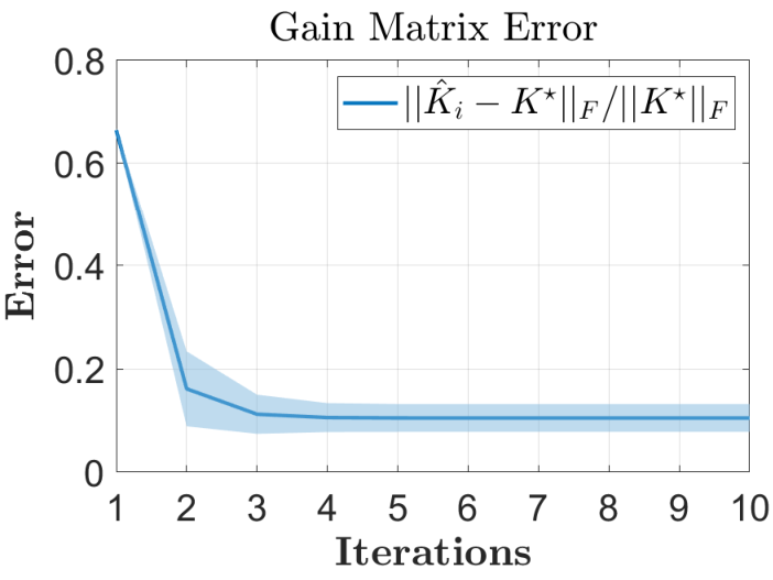
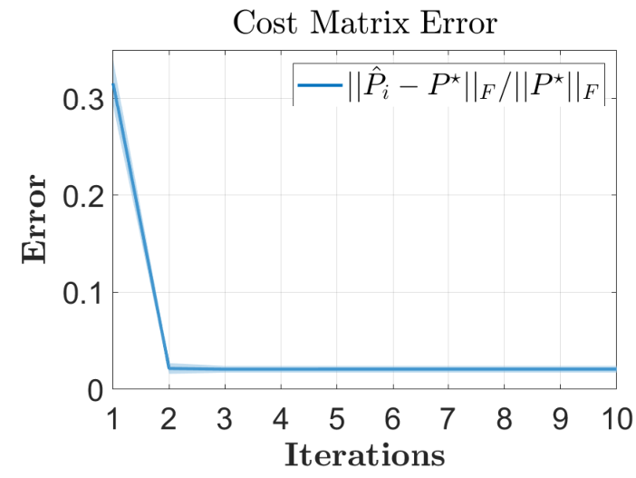
The robustness of Algorithm 1 in the presence of disturbance is validated first. For each outer and inner loop iteration, the entries of the disturbances Δ​Ki\Delta K_{i} and Δ​Li,j\Delta L_{i,j} are taken as samples from a standard Gaussian distribution and then their Frobenius norms are normalized to 0.090.09. The algorithm is run independently for 5050 times. The relative errors of the gain matrix K^i\hat{K}_{i} and cost matrix P^i\hat{P}_{i}, and the ℋ∞\mathcal{H}_{\infty} norm of the closed-loop system with K^i\hat{K}_{i} are shown in Fig. 2, where the bold line is the mean of the trials and the shaded region denotes the variance. It is seen that with the disturbances at both the outer and inner loop iterations, the generated controller and the corresponding cost matrix approach the optimal solution and finally enter a neighborhood of the optimal controller K∗K^{*} and cost matrix P∗P^{*}, respectively. The ℋ∞\mathcal{H}_{\infty} norm of the closed-loop system is smaller than the threshold throughout the policy optimization. These numerical results are consistent with the developed theoretical results in Theorems 4 and 5.

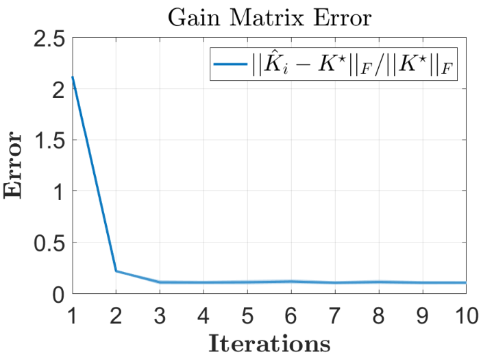
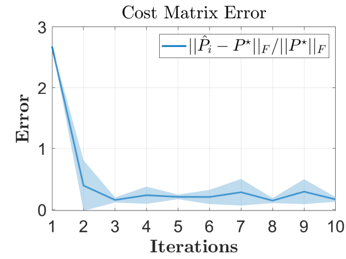
Algorithm 2 is implemented independently for 5050 trials to validate its performance. The length of the trajectory samples is τ=5000\tau=5000. The standard deviation of the system additive noise is Σ=I3\Sigma=I_{3}. The standard deviation of the exploratory noise is σ1=σ2=1\sigma_{1}=\sigma_{2}=1. The relative errors of the gain matrix and cost matrix are shown in Fig. 3. It is seen that the proposed off-policy RL algorithm can still approximate the optimal solution when the system is disturbed by additive Gaussian noise.
Refer to caption
Refer to caption
Refer to caption
Fig. 2: Robustness of Algorithm 1 when ∥Δ​K∥∞=0.09\lVert\Delta K\rVert_{\infty}=0.09 and ∥Δ​Li∥∞=0.09\lVert\Delta L_{i}\rVert_{\infty}=0.09.
Refer to caption
Refer to caption
Refer to caption
Fig. 3: Using Algorithm 2, the solutions of each iteration approach the optimal solution, and the ℋ∞\mathcal{H}_{\infty} norm is smaller than the threshold.

VI-B Cart-Pole Example

We next consider the cart-pole system in [48], where the inverted pendulum is hinged to the top of a wheeled cart that moves along a straight line. The rotational angle is denoted as ϕ\phi and the horizontal position is denoted by ss. The mass of the cart is mc=1​k​gm_{c}=1kg; the mass of the pendulum is mp=0.1​k​gm_{p}=0.1kg; the distance from the pendulum’s center of mass to the pivot is l=0.5​ml=0.5m; the gravitational acceleration is g=9.8​m/s​e​c2g=9.8m/sec^{2}. The system is discretized under the sampling period Δ​t=0.01​s​e​c\Delta t=0.01sec. Considering the noise for the system, the system can be described by a linear system with x=[s,s˙,ϕ,ϕ˙]Tx=[s,\dot{s},\phi,\dot{\phi}]^{T},

A=[10.010001−0.0100010.01000.161],B=[00.010−0.015],\displaystyle A=\begin{bmatrix}1&0.01&0&0\\ 0&1&-0.01&0\\ 0&0&1&0.01\\ 0&0&0.16&1\end{bmatrix},B=\begin{bmatrix}0\\ 0.01\\ 0\\ -0.015\end{bmatrix},

C=[I4,01×4]TC=[I_{4},0_{1\times 4}]^{T}, D=0.001​I4D=0.001I_{4}, E=[01×4,1]E=[0_{1\times 4},1]. The ℋ∞\mathcal{H}_{\infty} norm threshold is γ=10\gamma=10.

The robustness evaluation of Algorithm 1 is shown in Fig. 4, where the mean-variance curves are plotted for 5050 independent trials. At each iteration, the entries of the disturbances Δ​Ki\Delta K_{i} and Δ​Li,j\Delta L_{i,j} are randomly sampled from a standard Gaussian distribution, and then ∥Δ​Ki∥F\lVert\Delta K_{i}\rVert_{F} and ∥Δ​Li,j∥F\lVert\Delta L_{i,j}\rVert_{F} are normalized to 0.70.7 and 0.10.1, respectively. The relative errors approach zero even in the presence of the disturbance, demonstrating the small-disturbance ISS properties of the outer and inner loops in Theorems 4 and 5. In addition, the ℋ∞\mathcal{H}_{\infty} norm of the system is below the given threshold, and the robustness of the closed-loop system is guaranteed during the iteration.

When the matrices (A,B,D)(A,B,D) are unknown, Algorithm 2 is implemented independently for 5050 times. The length of the sampled trajectory is τ=10000\tau=10000, the standard deviation of the system additive noise is Σ=0.1​I4\Sigma=0.1I_{4}. The standard deviation of the exploratory noise is σ1=σ2=20\sigma_{1}=\sigma_{2}=20. It is seen from Fig. 5 that using the noisy data, the learning-based PO developed in Algorithm 2 still finds a near-optimal solution.

Refer to caption
Refer to caption
Refer to caption
Fig. 4: For the cart-pole system, the robustness of Algorithm 1 when ∥Δ​K∥∞=0.7\lVert\Delta K\rVert_{\infty}=0.7 and ∥Δ​Li∥∞=0.1\lVert\Delta L_{i}\rVert_{\infty}=0.1.
Refer to caption
Refer to caption
Refer to caption
Fig. 5: For the cart-pole system, as the iteration of Algorithm 2 proceeds, the gain and cost matrices approach the optimal solution, and the ℋ∞\mathcal{H}_{\infty} norm is smaller than the threshold.

VII Conclusion

In this paper, we have proposed a novel dual-loop policy optimization algorithm for data-driven risk-sensitive linear quadratic Gaussian control whose convergence and robustness properties have been analyzed. We have shown that the iterative algorithm possesses the property of small-disturbance input-to-state stability, that is, starting from any initial admissible controller, the solutions of the proposed policy optimization algorithm ultimately enter a neighbourhood of the optimal solution, given that the disturbance is relatively small. Based on these model-based theoretical results, when the accurate system knowledge is unavailable, we have also proposed a novel off-policy policy optimization RL algorithm to learn from data robust optimal controllers. Numerical examples are provided and the efficacy of the proposed methods are demonstrated by an academic example and a benchmark cart-pole system. Future work will be directed toward investigating the input-to-state stability of standard gradient descent and natural gradient descent algorithms. In addition, by invoking small-gain theory, the application of learning-based risk-sensitive LQG control to decentralized control design of complex systems will be studied.

Appendix A: Useful Auxiliary Results

Some fundamental lemmas are introduced to assist in the development of the results in the main body of the paper.

Lemma 1.

[49, Theorem 5.D6] Consider a stable matrix A∈ℝn×nA\in\mathbb{R}^{n\times n} satisfying

AT​P​A−P+Q=0.\displaystyle A^{T}PA-P+Q=0. (A.1)

The following statements hold:

  1. 1.

    P=∑t=0∞(AT)t​Q​AtP=\sum_{t=0}^{\infty}(A^{T})^{t}QA^{t} is the unique solution to (A.1) and P=PT⪰0P=P^{T}\succeq 0 if Q⪰0Q\succeq 0;

  2. 2.

    For any other P′=P′T⪰0P^{\prime}=P^{\prime T}\succeq 0 satisfying AT​P′​A−P′+Q′=0A^{T}P^{\prime}A-P^{\prime}+Q^{\prime}=0 with Q′⪰QQ^{\prime}\succeq Q, P′⪰PP^{\prime}\succeq P.

Lemma 2 (Bounded Real Lemma).

Given a matrix K∈ℝm×nK\in\mathbb{R}^{m\times n} and the transfer function 𝒯⁡(K)\mathcal{T}(K) for the linear system (1) under Assumptions 1 and 2, the following statements are equivalent:
1) KK is stabilizing and ∥𝒯⁡(K)∥ℋ∞<γ\lVert\mathcal{T}(K)\rVert_{\mathcal{H}_{\infty}}<\gamma;
2) The algebraic Riccati equation (4) admits a unique stabilizing solution PK=PKT≻0P_{K}=P_{K}^{T}\succ 0 such that i) Iq−γ−2​DT​PK​D≻0I_{q}-\gamma^{-2}D^{T}P_{K}D\succ 0; ii) [A−B​K+D​(γ2​Iq−DT​PK​D)−1​DT​PK​(A−B​K)][A-BK+D(\gamma^{2}I_{q}-D^{T}P_{K}D)^{-1}D^{T}P_{K}(A-BK)] is stable;
3) There exists PK=PKT≻0P_{K}=P_{K}^{T}\succ 0 such that

Iq−γ−2​DT​PK​D≻0,\displaystyle I_{q}-\gamma^{-2}D^{T}P_{K}D\succ 0, (A.2)
(A−B​K)T​UK​(A−B​K)−PK+Q+KT​R​K≺0.\displaystyle(A-BK)^{T}U_{K}(A-BK)-P_{K}+Q+K^{T}RK\prec 0.

4) There exist W=WT≻0W=W^{T}\succ 0 and V=K​WV=KW, such that

[−W∗∗∗0−γ2​Iq∗∗A​W−B​VD−W∗C​W−E​V00−Ip]≺0.\displaystyle\begin{bmatrix}-W&*&*&*\\ 0&-\gamma^{2}I_{q}&*&*\\ AW-BV&D&-W&*\\ CW-EV&0&0&-I_{p}\end{bmatrix}\prec 0. (A.3)
Proof.

The equivalence of the first three statements is from [35, Lemma 2.7]. We next prove the statement 4). By the Schur complement lemma, (A.3) is equivalent to

−W−[0W​AT−VT​BTW​CT−VT​ET]​[−γ2​IqDT0D−W000−Ip]−1​[0A​W−B​VC​W−E​V]≺0,\displaystyle-W-\begin{bmatrix}0&WA^{T}-V^{T}B^{T}&WC^{T}-V^{T}E^{T}\end{bmatrix}\begin{bmatrix}-\gamma^{2}I_{q}&D^{T}&0\\ D&-W&0\\ 0&0&-I_{p}\end{bmatrix}^{-1}\begin{bmatrix}0\\ AW-BV\\ CW-EV\end{bmatrix}\prec 0, (A.4a)
[−γ2​IqDT0D−W000−Ip]≺0.\displaystyle\begin{bmatrix}-\gamma^{2}I_{q}&D^{T}&0\\ D&-W&0\\ 0&0&-I_{p}\end{bmatrix}\prec 0. (A.4b)

Pre-multiplying and post-multiplying (A.4a) by P=W−1P=W^{-1}, and applying Schur complement on (A.4b), it is found that (A.4) is equivalent to

−P−[0(A−B​K)T(C−E​K)T]​[−γ2​IqDT0D−W000−Ip]−1​[0A−B​KC−E​K]≺0,\displaystyle-P-\begin{bmatrix}0&(A-BK)^{T}&(C-EK)^{T}\end{bmatrix}\begin{bmatrix}-\gamma^{2}I_{q}&D^{T}&0\\ D&-W&0\\ 0&0&-I_{p}\end{bmatrix}^{-1}\begin{bmatrix}0\\ A-BK\\ C-EK\end{bmatrix}\prec 0, (A.5a)
−γ2​Iq+DT​P​D≺0.\displaystyle-\gamma^{2}I_{q}+D^{T}PD\prec 0. (A.5b)

By recalling (C−E​K)T​(C−E​K)=Q+KT​R​K(C-EK)^{T}(C-EK)=Q+K^{T}RK, it follows that (A.5) is equivalent to (A.2). Thus, the proof is completed. ∎

Lemma 3.

For any positive semi-definite matrix P∈𝕊nP\in\mathbb{S}^{n}, ∥P∥F≤Tr⁡(P)≤n​∥P∥F\lVert P\rVert_{F}\leq\Tr(P)\leq\sqrt{n}\lVert P\rVert_{F} and ∥P∥≤Tr⁡(P)≤n⁡∥P∥\lVert P\rVert\leq\Tr(P)\leq n\lVert P\rVert.

Proof.

Let σ1≥⋯≥σn\sigma_{1}\geq\cdots\geq\sigma_{n} denote the descending sequence of PP’s singular values. Then, ∥P∥F=∑i=1nσi2\lVert P\rVert_{F}=\sqrt{\sum_{i=1}^{n}\sigma_{i}^{2}}, Tr⁡(P)=∑i=1nσi\Tr(P)=\sum_{i=1}^{n}\sigma_{i}, and ∥P∥=σ1​(P)\lVert P\rVert=\sigma_{1}(P). Hence, ∥P∥≤Tr⁡(P)≤n⁡∥P∥\lVert P\rVert\leq\Tr(P)\leq n\lVert P\rVert. ∥P∥F≤Tr⁡(P)≤n​∥P∥F\lVert P\rVert_{F}\leq\Tr(P)\leq\sqrt{n}\lVert P\rVert_{F} can be proven by the fact that ∑i=1nσi2≤(∑i=1nσi)2≤n​∑i=1nσi2\sum_{i=1}^{n}\sigma_{i}^{2}\leq(\sum_{i=1}^{n}\sigma_{i})^{2}\leq n\sum_{i=1}^{n}\sigma_{i}^{2}. ∎

Lemma 4.

There exists a unique matrix Tn∈ℝn2×12​n​(n+1)T_{n}\in\mathbb{R}^{n^{2}\times\frac{1}{2}n(n+1)} with full column rank, such that for every X∈𝕊nX\in\mathbb{S}^{n},

vec⁡(X)=Tn​vecs⁡(X),vecs⁡(X)=Tn†​vec⁡(X).\displaystyle\vect(X)=T_{n}\vecs(X),\quad\vecs(X)=T_{n}^{\dagger}\vect(X). (A.6)
Proof.

See [50, pp. 56] where TnT_{n} is called duplication matrix. ∎

Appendix B: Proof of Theorem 1

The following lemma shows that the cost matrix PiP_{i} generated by the outer-loop iteration (17) is monotonically decreasing and all the updated feedback gains are admissible given an initial admissible feedback gain.

Lemma 5.

Under Assumptions 1 and 2, if K1∈𝒲K_{1}\in\mathcal{W}, then for any i∈ℤ+i\in\mathbb{Z}_{+},

  1. 1.

    Ki∈𝒲K_{i}\in\mathcal{W};

  2. 2.

    P1⪰⋯⪰Pi⪰Pi+1⪰⋯⪰P∗P_{1}\succeq\cdots\succeq P_{i}\succeq P_{i+1}\succeq\cdots\succeq P^{*};

  3. 3.

    limi→∞∥Ki−K∗∥F=0\lim_{i\to\infty}\lVert K_{i}-K^{*}\rVert_{F}=0 and limi→∞∥Pi−P∗∥F=0\lim_{i\to\infty}\lVert P_{i}-P^{*}\rVert_{F}=0.

Proof.

The statements 1) and 3) are shown in [35, Theorem 4.3 and Theorem 4.6]. The statement 2) follows from [35, Equation (5.27)]. ∎

The following lemma presents the difference between the updated controller K′K^{\prime} and the optimal controller K∗K^{*}.

Lemma 6.

For any K∈𝒲K\in\mathcal{W} and K′:=(R+BT​UK​B)−1​BT​UK​AK^{\prime}:=(R+B^{T}U_{K}B)^{-1}B^{T}U_{K}A, we have

K′−K∗=R−1​BT​(ΛK)−T​(PK−P∗)​A∗,\displaystyle K^{\prime}-K^{*}=R^{-1}B^{T}(\Lambda_{K})^{-T}(P_{K}-P^{*})A^{*}, (B.1)
ΛK:=In+B​R−1​BT​PK−γ−2​D​DT​PK\displaystyle\Lambda_{K}:=I_{n}+BR^{-1}B^{T}P_{K}-\gamma^{-2}DD^{T}P_{K} (B.2)
Proof.

By the expression of UKU_{K} in (4b), we have

(R+BT​UK​B)−1​BT​UK​A=R−1​(Im+BT​UK​B​R−1)−1​BT​UK​A=R−1​BT​UK​(In+B​R−1​BT​UK)−1​A=R−1​BT​UK​[In+B​R−1​BT​PK+B​R−1​BT​PK​D​(γ2​Iq−DT​PK​D)−1​DT​PK]−1​A=R−1​BT​UK​{In+B​R−1​BT​PK​[In+D​DT​PK​(γ2​In−D​DT​PK)−1]}−1​A=R−1​BT​UK​[In+B​R−1​BT​PK​(In−γ−2​D​DT​PK)−1]−1​A=R−1​BT​UK​(In−γ−2​D​DT​PK)​(In+B​R−1​BT​PK−γ−2​D​DT​PK)−1​A=R−1​BT​PK​[In+D​(γ2​Iq−DT​PK​D)−1​DT​PK]​(In−γ−2​D​DT​PK)​ΛK−1​A=R−1​BT​PK​[In+γ−2​D​DT​PK​(In−γ−2​D​DT​PK)−1]​(In−γ−2​D​DT​PK)​ΛK−1​A=R−1​BT​PK​ΛK−1​A.\displaystyle\begin{split}&(R+B^{T}U_{K}B)^{-1}B^{T}U_{K}A=R^{-1}(I_{m}+B^{T}U_{K}BR^{-1})^{-1}B^{T}U_{K}A\\ &\qquad=R^{-1}B^{T}U_{K}(I_{n}+BR^{-1}B^{T}U_{K})^{-1}A\\ &\qquad=R^{-1}B^{T}U_{K}[I_{n}+BR^{-1}B^{T}P_{K}+BR^{-1}B^{T}P_{K}D(\gamma^{2}I_{q}-D^{T}P_{K}D)^{-1}D^{T}P_{K}]^{-1}A\\ &\qquad=R^{-1}B^{T}U_{K}\{I_{n}+BR^{-1}B^{T}P_{K}[I_{n}+DD^{T}P_{K}(\gamma^{2}I_{n}-DD^{T}P_{K})^{-1}]\}^{-1}A\\ &\qquad=R^{-1}B^{T}U_{K}[I_{n}+BR^{-1}B^{T}P_{K}(I_{n}-\gamma^{-2}DD^{T}P_{K})^{-1}]^{-1}A\\ &\qquad=R^{-1}B^{T}U_{K}(I_{n}-\gamma^{-2}DD^{T}P_{K})(I_{n}+BR^{-1}B^{T}P_{K}-\gamma^{-2}DD^{T}P_{K})^{-1}A\\ &\qquad=R^{-1}B^{T}P_{K}[I_{n}+D(\gamma^{2}I_{q}-D^{T}P_{K}D)^{-1}D^{T}P_{K}](I_{n}-\gamma^{-2}DD^{T}P_{K})\Lambda_{K}^{-1}A\\ &\qquad=R^{-1}B^{T}P_{K}[I_{n}+\gamma^{-2}DD^{T}P_{K}(I_{n}-\gamma^{-2}DD^{T}P_{K})^{-1}](I_{n}-\gamma^{-2}DD^{T}P_{K})\Lambda_{K}^{-1}A\\ &\qquad=R^{-1}B^{T}P_{K}\Lambda_{K}^{-1}A.\end{split} (B.3)

By the expressions of K′K^{\prime} and K∗K^{*} in (5), we have

K′−K∗=R−1​BT​PK​ΛK−1​A−R−1​BT​P∗​(Λ∗)−1​A\displaystyle K^{\prime}-K^{*}=R^{-1}B^{T}P_{K}\Lambda_{K}^{-1}A-R^{-1}B^{T}P^{*}(\Lambda^{*})^{-1}A (B.4)
=R−1​BT​(PK−P∗)​(Λ∗)−1​A+R−1​BT​PK​ΛK−1​A−R−1​BT​PK​(Λ∗)−1​A\displaystyle\quad=R^{-1}B^{T}(P_{K}-P^{*})(\Lambda^{*})^{-1}A+R^{-1}B^{T}P_{K}\Lambda_{K}^{-1}A-R^{-1}B^{T}P_{K}(\Lambda^{*})^{-1}A
=R−1​BT​(PK−P∗)​(Λ∗)−1​A+R−1​BT​PK​[ΛK−1​Λ∗​(Λ∗)−1−ΛK−1​ΛK​(Λ∗)−1]​A\displaystyle\quad=R^{-1}B^{T}(P_{K}-P^{*})(\Lambda^{*})^{-1}A+R^{-1}B^{T}P_{K}\left[\Lambda_{K}^{-1}\Lambda^{*}(\Lambda^{*})^{-1}-\Lambda_{K}^{-1}\Lambda_{K}(\Lambda^{*})^{-1}\right]A
=R−1​BT​(PK−P∗)​(Λ∗)−1​A−R−1​BT​PK​ΛK−1​(B​R−1​BT−γ−2​D​DT)​(PK−P∗)​(Λ∗)−1​A\displaystyle\quad=R^{-1}B^{T}(P_{K}-P^{*})(\Lambda^{*})^{-1}A-R^{-1}B^{T}P_{K}\Lambda_{K}^{-1}(BR^{-1}B^{T}-\gamma^{-2}DD^{T})(P_{K}-P^{*})(\Lambda^{*})^{-1}A
=R−1​BT​[In−PK​ΛK−1​(B​R−1​BT−γ−2​D​DT)]​(PK−P∗)​A∗\displaystyle\quad=R^{-1}B^{T}[I_{n}-P_{K}\Lambda_{K}^{-1}(BR^{-1}B^{T}-\gamma^{-2}DD^{T})](P_{K}-P^{*})A^{*}
=R−1​BT​[In−(In+PK​B​R−1​BT−γ−2​PK​D​DT)−1​PK​(B​R−1​BT−γ−2​D​DT)]​(PK−P∗)​A∗\displaystyle\quad=R^{-1}B^{T}[I_{n}-(I_{n}+P_{K}BR^{-1}B^{T}-\gamma^{-2}P_{K}DD^{T})^{-1}P_{K}(BR^{-1}B^{T}-\gamma^{-2}DD^{T})](P_{K}-P^{*})A^{*}
=R−1​BT​(In+PK​B​R−1​BT−γ−2​PK​D​DT)−1​(PK−P∗)​A∗=R−1​BT​(ΛK)−T​(PK−P∗)​A∗.\displaystyle\quad=R^{-1}B^{T}(I_{n}+P_{K}BR^{-1}B^{T}-\gamma^{-2}P_{K}DD^{T})^{-1}(P_{K}-P^{*})A^{*}=R^{-1}B^{T}(\Lambda_{K})^{-T}(P_{K}-P^{*})A^{*}.

It is noticed that the fifth equation follows from the equality

A∗\displaystyle A^{*} =[In+D​(γ2​Iq−DT​P∗​D)−1​DT​P∗]​(A−B​K∗)=(In−γ−2​D​DT​P∗)−1​(A−B​K∗)\displaystyle=[I_{n}+D(\gamma^{2}I_{q}-D^{T}P^{*}D)^{-1}D^{T}P^{*}](A-BK^{*})=(I_{n}-\gamma^{-2}DD^{T}P^{*})^{-1}(A-BK^{*})
=(In−γ−2​D​DT​P∗)−1​[In−B​(R+BT​U∗​B)−1​BT​U∗]​A\displaystyle=(I_{n}-\gamma^{-2}DD^{T}P^{*})^{-1}[I_{n}-B(R+B^{T}U^{*}B)^{-1}B^{T}U^{*}]A
=(In−γ−2​D​DT​P∗)−1​(In+B​R−1​BT​U∗)−1​A\displaystyle=(I_{n}-\gamma^{-2}DD^{T}P^{*})^{-1}(I_{n}+BR^{-1}B^{T}U^{*})^{-1}A (B.5)
=(In−γ−2​D​DT​P∗)−1​[In+B​R−1​BT​P∗​(In−γ−2​D​DT​P∗)−1]−1​A=(Λ∗)−1​A.\displaystyle=(I_{n}-\gamma^{-2}DD^{T}P^{*})^{-1}[I_{n}+BR^{-1}B^{T}P^{*}(I_{n}-\gamma^{-2}DD^{T}P^{*})^{-1}]^{-1}A=(\Lambda^{*})^{-1}A.

∎

The following lemma presents the expression of the difference between UKU_{K} and U∗U^{*}.

Lemma 7.

For any K∈𝒲K\in\mathcal{W}, (UK−U∗)(U_{K}-U^{*}) satisfies

UK−U∗\displaystyle U_{K}-U^{*}
=(In−γ−2​P∗​D​DT)−1​(PK−P∗)​(In−γ−2​D​DT​P∗)−1\displaystyle=(I_{n}-\gamma^{-2}P^{*}DD^{T})^{-1}(P_{K}-P^{*})(I_{n}-\gamma^{-2}DD^{T}P^{*})^{-1}
+(In−γ−2​P∗​D​DT)−1​(PK−P∗)​D​(γ2​Iq−DT​PK​D)−1\displaystyle+(I_{n}-\gamma^{-2}P^{*}DD^{T})^{-1}(P_{K}-P^{*})D(\gamma^{2}I_{q}-D^{T}P_{K}D)^{-1}
DT​(PK−P∗)​(In−γ−2​D​DT​P∗)−1\displaystyle\quad D^{T}(P_{K}-P^{*})(I_{n}-\gamma^{-2}DD^{T}P^{*})^{-1} (B.6)
Proof.

By recalling the expression of U∗U^{*} in (6), we can further derive it as

U∗=[In+P∗​D​(γ2​Iq−DT​P∗​D)−1​DT]​P∗=[In+P∗​D​DT​(γ2​In−P∗​D​DT)−1]​P∗\displaystyle U^{*}=[I_{n}+P^{*}D(\gamma^{2}I_{q}-D^{T}P^{*}D)^{-1}D^{T}]P^{*}=[I_{n}+P^{*}DD^{T}(\gamma^{2}I_{n}-P^{*}DD^{T})^{-1}]P^{*}
=(In−γ−2​P∗​D​DT)−1​P∗=(In−γ−2​P∗​D​DT)−1​P∗​(In−γ−2​D​DT​P∗)​(In−γ−2​D​DT​P∗)−1\displaystyle=(I_{n}-\gamma^{-2}P^{*}DD^{T})^{-1}P^{*}=(I_{n}-\gamma^{-2}P^{*}DD^{T})^{-1}P^{*}(I_{n}-\gamma^{-2}DD^{T}P^{*})(I_{n}-\gamma^{-2}DD^{T}P^{*})^{-1}
=(In−γ−2​P∗​D​DT)−1​(PK−γ−2​P∗​D​DT​P∗)​(In−γ−2​D​DT​P∗)−1\displaystyle=(I_{n}-\gamma^{-2}P^{*}DD^{T})^{-1}(P_{K}-\gamma^{-2}P^{*}DD^{T}P^{*})(I_{n}-\gamma^{-2}DD^{T}P^{*})^{-1}
−(In−γ−2​P∗​D​DT)−1​(PK−P∗)​(In−γ−2​D​DT​P∗)−1.\displaystyle-(I_{n}-\gamma^{-2}P^{*}DD^{T})^{-1}(P_{K}-P^{*})(I_{n}-\gamma^{-2}DD^{T}P^{*})^{-1}. (B.7)

To simplify the notation, define SKS_{K} as

SK:=UK−(In−γ−2​P∗​D​DT)−1​(PK−γ−2​P∗​D​DT​P∗)​(In−γ−2​D​DT​P∗)−1.\displaystyle S_{K}:=U_{K}-(I_{n}-\gamma^{-2}P^{*}DD^{T})^{-1}(P_{K}-\gamma^{-2}P^{*}DD^{T}P^{*})(I_{n}-\gamma^{-2}DD^{T}P^{*})^{-1}. (B.8)

Then, it follows that

(In−γ−2​P∗​D​DT)​SK​(In−γ−2​D​DT​P∗)\displaystyle(I_{n}-\gamma^{-2}P^{*}DD^{T})S_{K}(I_{n}-\gamma^{-2}DD^{T}P^{*}) (B.9)
=(In−γ−2​P∗​D​DT)​UK​(In−γ−2​D​DT​P∗)−(PK−γ−2​P∗​D​DT​P∗)\displaystyle=(I_{n}-\gamma^{-2}P^{*}DD^{T})U_{K}(I_{n}-\gamma^{-2}DD^{T}P^{*})-(P_{K}-\gamma^{-2}P^{*}DD^{T}P^{*})
=UK−PK−γ−2​P∗​D​DT​UK−γ−2​UK​D​DT​P∗+γ−4​P∗​D​DT​UK​D​DT​P∗+γ−2​P∗​D​DT​P∗.\displaystyle=U_{K}-P_{K}-\gamma^{-2}P^{*}DD^{T}U_{K}-\gamma^{-2}U_{K}DD^{T}P^{*}+\gamma^{-4}P^{*}DD^{T}U_{K}DD^{T}P^{*}+\gamma^{-2}P^{*}DD^{T}P^{*}.

Following the expression of UKU_{K} in (4b), we have

γ−2​P∗​D​DT​UK\displaystyle\gamma^{-2}P^{*}DD^{T}U_{K} (B.10)
=γ−2​P∗​D​DT​(In−γ−2​PK​D​DT)−1​PK=γ−2​P∗​D​(Iq−γ−2​DT​PK​D)−1​DT​PK.\displaystyle=\gamma^{-2}P^{*}DD^{T}(I_{n}-\gamma^{-2}P_{K}DD^{T})^{-1}P_{K}=\gamma^{-2}P^{*}D(I_{q}-\gamma^{-2}D^{T}P_{K}D)^{-1}D^{T}P_{K}.

Since UK−PK=PK​D​(γ2​Iq−DT​PK​D)−1​DT​PKU_{K}-P_{K}=P_{K}D(\gamma^{2}I_{q}-D^{T}P_{K}D)^{-1}D^{T}P_{K}, plugging (B.10) into (B.9) and completing the squares yield

(In−γ−2​P∗​D​DT)​SK​(In−γ−2​D​DT​P∗)=(PK−P∗)​D​(γ2​Iq−DT​PK​D)−1​DT​(PK−P∗)\displaystyle(I_{n}-\gamma^{-2}P^{*}DD^{T})S_{K}(I_{n}-\gamma^{-2}DD^{T}P^{*})=(P_{K}-P^{*})D(\gamma^{2}I_{q}-D^{T}P_{K}D)^{-1}D^{T}(P_{K}-P^{*})
−P∗​D​(γ2​Iq−DT​PK​D)−1​DT​P∗+γ−4​P∗​D​DT​UK​D​DT​P∗+γ−2​P∗​D​DT​P∗.\displaystyle\qquad-P^{*}D(\gamma^{2}I_{q}-D^{T}P_{K}D)^{-1}D^{T}P^{*}+\gamma^{-4}P^{*}DD^{T}U_{K}DD^{T}P^{*}+\gamma^{-2}P^{*}DD^{T}P^{*}. (B.11)

By the matrix inversion lemma,

(γ2​Iq−DT​PK​D)−1=γ−2​Iq+γ−4​DT​(In−γ−2​PK​D​DT)−1​PK​D=γ−2​Iq+γ−4​DT​UK​D,\displaystyle(\gamma^{2}I_{q}-D^{T}P_{K}D)^{-1}=\gamma^{-2}I_{q}+\gamma^{-4}D^{T}(I_{n}-\gamma^{-2}P_{K}DD^{T})^{-1}P_{K}D=\gamma^{-2}I_{q}+\gamma^{-4}D^{T}U_{K}D, (B.12)

where the last equality is from UK=(In−γ−2​PK​D​DT)−1​PKU_{K}=(I_{n}-\gamma^{-2}P_{K}DD^{T})^{-1}P_{K}. Plugging (B.12) into (Proof.), we have

SK=(In−γ−2​P∗​D​DT)−1​(PK−P∗)​D​(γ2​Iq−DT​PK​D)−1​DT​(PK−P∗)​(In−γ−2​D​DT​P∗)−1.\displaystyle S_{K}=(I_{n}-\gamma^{-2}P^{*}DD^{T})^{-1}(P_{K}-P^{*})D(\gamma^{2}I_{q}-D^{T}P_{K}D)^{-1}D^{T}(P_{K}-P^{*})(I_{n}-\gamma^{-2}DD^{T}P^{*})^{-1}. (B.13)

Therefore, (7) is obtained by (Proof.) and (B.13). ∎

Lemma 8.

For any K∈𝒲K\in\mathcal{W}, PKP_{K} is continuous with respect to KK, where PKP_{K} is the unique positive-definite solution to (4).

Proof.

The lemma follows from the implicit function theorem. Consider the function

F⁡(K,PK):=(A−B​K)T​UK​(A−B​K)−PK+Q+KT​R​K.\displaystyle\begin{split}&F(K,P_{K}):=(A-BK)^{T}U_{K}(A-BK)-P_{K}+Q+K^{T}RK.\end{split} (B.14)

Let ℱ⁡(vec⁡(K),vec⁡(PK)):=vec⁡(F⁡(K,PK))\mathcal{F}(\vect(K),\vect(P_{K})):=\vect(F(K,P_{K})). Then,

ℱ⁡(vec⁡(K),vec⁡(PK))=[(A−B​K)T⊗(A−B​K)T]​vec⁡(UK)−vec⁡(PK)+vec⁡(Q+KT​R​K).\displaystyle\begin{split}&\mathcal{F}(\vect(K),\vect(P_{K}))=[(A-BK)^{T}\otimes(A-BK)^{T}]\vect(U_{K})\\ &-\vect(P_{K})+\vect(Q+K^{T}RK).\end{split} (B.15)

Noticing UK=(In−γ−2​PK​D​DT)−1​PKU_{K}=(I_{n}-\gamma^{-2}P_{K}DD^{T})^{-1}P_{K} and [51, Theroem 9], we have

∂vec⁡(UK)∂vec⁡(PK)=(PK⊗In)​∂vec⁡((In−γ−2​PK​D​DT)−1)∂vec⁡(PK)\displaystyle\frac{\partial\vect(U_{K})}{\partial\vect(P_{K})}=(P_{K}\otimes I_{n})\frac{\partial\vect((I_{n}-\gamma^{-2}P_{K}DD^{T})^{-1})}{\partial\vect(P_{K})}
+[In⊗(In−γ−2​PK​D​DT)−1]​∂vec⁡(PK)∂vec⁡(PK)\displaystyle+[I_{n}\otimes(I_{n}-\gamma^{-2}P_{K}DD^{T})^{-1}]\frac{\partial\vect(P_{K})}{\partial\vect(P_{K})} (B.16)
={[γ−2PKDDT(In−γ−2PKDDT)−1]\displaystyle=\left\{[\gamma^{-2}P_{K}DD^{T}(I_{n}-\gamma^{-2}P_{K}DD^{T})^{-1}]\right.
⊗(I−γ−2PKDDT)−1}+[In⊗(In−γ−2PKDDT)−1]\displaystyle\quad\left.\otimes(I-\gamma^{-2}P_{K}DD^{T})^{-1}\right\}+[I_{n}\otimes(I_{n}-\gamma^{-2}P_{K}DD^{T})^{-1}]
=(In−γ−2​PK​D​DT)−1⊗(In−γ−2​PK​D​DT)−1,\displaystyle=(I_{n}-\gamma^{-2}P_{K}DD^{T})^{-1}\otimes(I_{n}-\gamma^{-2}P_{K}DD^{T})^{-1},

where the second equality follows from [35, Equation (B.10)]. Considering

LK,∗=(γ2​Iq−DT​PK​D)−1​DT​PK​(A−B​K)\displaystyle L_{K,*}=(\gamma^{2}I_{q}-D^{T}P_{K}D)^{-1}D^{T}P_{K}(A-BK) (B.17)
A−B​K+D​LK,∗=(In−γ−2​D​DT​PK)−1​(A−B​K),\displaystyle A-BK+DL_{K,*}=(I_{n}-\gamma^{-2}DD^{T}P_{K})^{-1}(A-BK),

and plugging (Proof.) and (B.17) into the derivative of (B.15) yield

∂ℱ⁡(vec⁡(K),vec⁡(PK))∂vec⁡(PK)=[(A−BK+DLK,∗)T⊗(A−BK+DLK,∗)T]−In2.\displaystyle\begin{split}&\frac{\partial\mathcal{F}(\vect(K),\vect(P_{K}))}{\partial\vect(P_{K})}=[(A-BK+DL_{K,*})^{T}\\ &\otimes(A-BK+DL_{K,*})^{T}]-I_{n^{2}}.\end{split} (B.18)

Since K∈𝒲K\in\mathcal{W}, by Lemma 2, (A−B​K+D​LK,∗)(A-BK+DL_{K,*}) is stable. Then, ∂ℱ⁡(vec⁡(K),vec⁡(PK))∂vec⁡(PK)\frac{\partial\mathcal{F}(\vect(K),\vect(P_{K}))}{\partial\vect(P_{K})} is invertible since σ¯​(A−B​K+D​LK,∗)<1\bar{\sigma}(A-BK+DL_{K,*})<1. By the implicit function theorem, PKP_{K} is continuous with respect to KK for any K∈𝒲K\in\mathcal{W}. ∎

Lemma 9.

Let K∈𝒲K\in\mathcal{W}, PKP_{K} be the positive-definite solution of (4a), and K′=(R+BT​UK​B)−1​BT​UK​AK^{\prime}=(R+B^{T}U_{K}B)^{-1}B^{T}U_{K}A. Then, (K−K′)T​R​(K−K′)=0(K-K^{\prime})^{T}R(K-K^{\prime})=0 is equivalent to K=K∗K=K^{*}.

Proof.

(⇒\Rightarrow): Since R≻0R\succ 0, (K−K′)T​R​(K−K′)=0(K-K^{\prime})^{T}R(K-K^{\prime})=0 implies K=K′K=K^{\prime}. From (4a), we have

(A−B​K)T​UK​(A−B​K)−PK+Q+KT​R​K=0\displaystyle(A-BK)^{T}U_{K}(A-BK)-P_{K}+Q+K^{T}RK=0
K=(R+BT​U​B)−1​BT​UK​A.\displaystyle K=(R+B^{T}UB)^{-1}B^{T}U_{K}A. (B.19)

Hence, PK≻0P_{K}\succ 0 satisfies the GARE (6). Due to the uniqueness of the positive-definite solution to (6), it is deduced that PK=P∗P_{K}=P^{*} and K=K∗K=K^{*}.

(⇐\Leftarrow): Since K=K∗K=K^{*} and PK=P∗P_{K}=P^{*}, it follows that K′=(R+BT​UK​B)−1​BT​UK​A=KK^{\prime}=(R+B^{T}U_{K}B)^{-1}B^{T}U_{K}A=K. Hence, K=K′K=K^{\prime} and (K−K′)T​R​(K−K′)=0(K-K^{\prime})^{T}R(K-K^{\prime})=0. ∎

Lemma 10.

For any h∈ℋh\in\mathcal{H}, 𝒢h:={K∈𝒲|Tr⁡(PK)≤Tr⁡(P∗)+h}\mathcal{G}_{h}:=\{K\in\mathcal{W}|\Tr(P_{K})\leq\Tr(P^{*})+h\} is compact.

Proof.

Firstly, we prove the boundedness of 𝒢h\mathcal{G}_{h}. For any K∈𝒢hK\in\mathcal{G}_{h}, PKP_{K} is bounded. Since UK⪰0U_{K}\succeq 0, it is seen from (4a) that KT​R​K⪯PKK^{T}RK\preceq P_{K}. As R≻0R\succ 0, KK is bounded.

Next, we prove the closeness of 𝒢h\mathcal{G}_{h}. Let {Ks}s=1∞\{K_{s}\}_{s=1}^{\infty} denote an arbitrary convergent sequence within 𝒢h\mathcal{G}_{h} and lims→∞∥Ks−Kl​i​m∥F=0\lim_{s\to\infty}\lVert K_{s}-K_{lim}\rVert_{F}=0. Since PKP_{K} is continuous with respect to KK (Lemma 8), we have lims→∞PKs=PKl​i​m\lim_{s\to\infty}P_{K_{s}}=P_{K_{lim}}. Since Tr⁡(PKs)≤Tr⁡(P∗)+h\Tr(P_{K_{s}})\leq\Tr(P^{*})+h, it follows that Tr⁡(PKl​i​m)≤Tr⁡(P∗)+h\Tr(P_{K_{lim}})\leq\Tr(P^{*})+h. In addition, PKl​i​m⪰0P_{K_{lim}}\succeq 0 is obtained by Lemma 2 and PKs⪰0P_{K_{s}}\succeq 0. Since the pair (Kl​i​m,PKl​i​mK_{lim},P_{K_{lim}}) satisfies (4a), Kl​i​m∈𝒲K_{lim}\in\mathcal{W} is obtained by Lemma 2. As a result, Kl​i​m∈𝒢hK_{lim}\in\mathcal{G}_{h} and 𝒢h\mathcal{G}_{h} is closed. In summary, the compactness of 𝒢h\mathcal{G}_{h} is demonstrated by Heine–Borel theorem. ∎

Lemma 11.

For any h∈ℋh\in\mathcal{H} and K∈𝒢hK\in\mathcal{G}_{h}, let K′:=(R+BT​UK​B)−1​BT​UK​AK^{\prime}:=(R+B^{T}U_{K}B)^{-1}B^{T}U_{K}A, and EK:=(K′−K)T​(R+BT​UK​B)​(K′−K)E_{K}:=(K^{\prime}-K)^{T}(R+B^{T}U_{K}B)(K^{\prime}-K). Then, there exists a⁡(h)>0a(h)>0, such that

∥PK−P∗∥F≤a⁡(h)​∥EK∥F.\displaystyle\begin{split}\lVert P_{K}-P^{*}\rVert_{F}\leq a(h)\lVert E_{K}\rVert_{F}.\end{split} (B.20)
Proof.

It follows from (4) that

(A−B​K∗)T​UK​(A−B​K∗)−PK+Q+KT​R​K+AT​UK​B​(K∗−K)+(K∗−K)T​BT​UK​A+KT​BT​UK​B​K−(K∗)T​BT​UK​B​K∗=0.\displaystyle\begin{split}&(A-BK^{*})^{T}U_{K}(A-BK^{*})-P_{K}+Q+K^{T}RK\\ &+A^{T}U_{K}B(K^{*}-K)+(K^{*}-K)^{T}B^{T}U_{K}A\\ &+K^{T}B^{T}U_{K}BK-(K^{*})^{T}B^{T}U_{K}BK^{*}=0.\end{split} (B.21)

Subtracting (6a) from (B.21), and considering BT​UK​A=(R+BT​UK​B)​K′B^{T}U_{K}A=(R+B^{T}U_{K}B)K^{\prime}, we have

(A−B​K∗)T​(UK−U∗)​(A−B​K∗)−(PK−P∗)\displaystyle(A-BK^{*})^{T}(U_{K}-U^{*})(A-BK^{*})-(P_{K}-P^{*})
+KT​(R+BT​UK​B)​K+(K′)T​(R+BT​UK​B)​(K∗−K)\displaystyle+K^{T}(R+B^{T}U_{K}B)K+(K^{\prime})^{T}(R+B^{T}U_{K}B)(K^{*}-K)
+(K∗−K)T​(R+BT​UK​B)​K′\displaystyle+(K^{*}-K)^{T}(R+B^{T}U_{K}B)K^{\prime}
−(K∗)T​(R+BT​UK​B)​K∗=0.\displaystyle-(K^{*})^{T}(R+B^{T}U_{K}B)K^{*}=0. (B.22)

Completing the squares in (Proof.) yields

(A−B​K∗)T​(UK−U∗)​(A−B​K∗)−(PK−P∗)+EK\displaystyle(A-BK^{*})^{T}(U_{K}-U^{*})(A-BK^{*})-(P_{K}-P^{*})+E_{K}
−(K′−K∗)T​(R+BT​UK​B)​(K′−K∗)=0.\displaystyle-(K^{\prime}-K^{*})^{T}(R+B^{T}U_{K}B)(K^{\prime}-K^{*})=0. (B.23)

It follows from (In−γ−2​D​DT​P∗)−1​(A−B​K∗)=(A−B​K∗+D​L∗)=A∗(I_{n}-\gamma^{-2}DD^{T}P^{*})^{-1}(A-BK^{*})=(A-BK^{*}+DL^{*})=A^{*} and Lemma 7 that

(A∗)T​Δ​PK​(A∗)−Δ​PK+EK\displaystyle(A^{*})^{T}\Delta P_{K}(A^{*})-\Delta P_{K}+E_{K}
−(K′−K∗)T​(R+BT​UK​B)​(K′−K∗)\displaystyle-(K^{\prime}-K^{*})^{T}(R+B^{T}U_{K}B)(K^{\prime}-K^{*}) (B.24)
+(A∗)T​Δ​PK​D​(γ2​Iq−DT​PK​D)−1​DT​Δ​PK​A∗=0.\displaystyle+(A^{*})^{T}\Delta P_{K}D(\gamma^{2}I_{q}-D^{T}P_{K}D)^{-1}D^{T}\Delta P_{K}A^{*}=0.

To simplify the notation, let Δ​PK:=PK−P∗\Delta P_{K}:=P_{K}-P^{*}. According to Lemma 1, we have

Δ​PK⪯∑k=0∞(A∗)T,k[EK+(A∗)TΔPKD(γ2Iq−DTPKD)−1DTΔPKA∗](A∗)k.\displaystyle\begin{split}\Delta P_{K}&\preceq\sum_{k=0}^{\infty}(A^{*})^{T,k}\left[E_{K}+(A^{*})^{T}\Delta P_{K}D\right.\\ &\left.(\gamma^{2}I_{q}-D^{T}P_{K}D)^{-1}D^{T}\Delta P_{K}A^{*}\right](A^{*})^{k}.\end{split} (B.25)

Taking the trace of (B.25) and using the cyclic property of trace and trace inequality in [52, Lemma 1] yields

Tr(ΔPK)≤Tr[∑k=0∞(A∗)k(A∗)T,kEK]+Tr[∑k=1∞(A∗)k\displaystyle\Tr(\Delta P_{K})\leq\Tr\left[\sum_{k=0}^{\infty}(A^{*})^{k}(A^{*})^{T,k}E_{K}\right]+\Tr\left[\sum_{k=1}^{\infty}(A^{*})^{k}\right.
(A∗)T,kΔPKD(γ2Iq−DTPKD)−1DTΔPK]\displaystyle\left.(A^{*})^{T,k}\Delta P_{K}D(\gamma^{2}I_{q}-D^{T}P_{K}D)^{-1}D^{T}\Delta P_{K}\right]
≤a1Tr(EK)+a2γ−2Tr[ΔPK\displaystyle\leq a_{1}\Tr(E_{K})+a_{2}\gamma^{-2}\Tr[\Delta P_{K}
(In−γ−2DDTPK)−1DDTΔPK],\displaystyle(I_{n}-\gamma^{-2}DD^{T}P_{K})^{-1}DD^{T}\Delta P_{K}], (B.26)

where

a1=∥∑k=0∞(A∗)k​(A∗)T,k∥,a2=∥∑k=1∞(A∗)k​(A∗)T,k∥.\displaystyle\begin{split}a_{1}&=\lVert\sum_{k=0}^{\infty}(A^{*})^{k}(A^{*})^{T,k}\rVert,\\ a_{2}&=\lVert\sum_{k=1}^{\infty}(A^{*})^{k}(A^{*})^{T,k}\rVert.\end{split} (B.27)

By Neumann series, for any X∈ℝn×nX\in\mathbb{R}^{n\times n} with ∥X∥<1\lVert X\rVert<1, it holds

∥(I−X)−1∥=∥∑k=0∞Xk∥≤11−∥X∥.\displaystyle\lVert(I-X)^{-1}\rVert=\lVert\sum_{k=0}^{\infty}X^{k}\rVert\leq\frac{1}{1-\lVert X\rVert}. (B.28)

Therefore, for small enough Δ​PK\Delta P_{K}, we have

∥(In−γ−2​D​DT​PK)−1∥\displaystyle\lVert(I_{n}-\gamma^{-2}DD^{T}P_{K})^{-1}\rVert
=∥(In−γ−2​D​DT​P∗−γ−2​D​DT​Δ​PK)−1∥\displaystyle=\lVert(I_{n}-\gamma^{-2}DD^{T}P^{*}-\gamma^{-2}DD^{T}\Delta P_{K})^{-1}\rVert (B.29)
≤∥(In−γ−2​D​DT​P∗)−1∥1−a3​∥Δ​PK∥.\displaystyle\leq\frac{\lVert(I_{n}-\gamma^{-2}DD^{T}P^{*})^{-1}\rVert}{1-a_{3}\lVert\Delta P_{K}\rVert}.

where

a3=γ−2​∥(In−γ−2​D​DT​P∗)−1∥​∥D​DT∥.\displaystyle a_{3}=\gamma^{-2}\lVert(I_{n}-\gamma^{-2}DD^{T}P^{*})^{-1}\rVert\lVert DD^{T}\rVert. (B.30)

Using the trace inequality in [52, Lemma 1], it follows from (Proof.) and (Proof.) that

(1−a2​a3​∥Δ​PK∥1−a3​∥Δ​PK∥)​Tr⁡(Δ​PK)≤a1​Tr⁡(EK).\displaystyle\left(1-\frac{a_{2}a_{3}\lVert\Delta P_{K}\rVert}{1-a_{3}\lVert\Delta P_{K}\rVert}\right)\Tr(\Delta P_{K})\leq a_{1}\Tr(E_{K}). (B.31)

Therefore, if

∥Δ​PK∥≤1a3+2​a2​a3=:h1,\displaystyle\lVert\Delta P_{K}\rVert\leq\frac{1}{a_{3}+2a_{2}a_{3}}=:h_{1}, (B.32)

it follows from Lemma 3 that

∥Δ​PK∥F≤Tr⁡(Δ​PK)≤2​a1​Tr⁡(EK)≤2​a1​n​∥EK∥F.\displaystyle\lVert\Delta P_{K}\rVert_{F}\leq\Tr(\Delta P_{K})\leq 2a_{1}\Tr(E_{K})\leq 2a_{1}\sqrt{n}\lVert E_{K}\rVert_{F}. (B.33)

When ∥Δ​PK∥≥h1\lVert\Delta P_{K}\rVert\geq h_{1}, if follows from Lemma 9 that ∥EK∥F≠0\lVert E_{K}\rVert_{F}\neq 0. Since EKE_{K} is continuous with respect to KK (Lemma 8) and the set 𝒢h∩{K∈𝒲|∥Δ​PK∥≥h1}\mathcal{G}_{h}\cap\{K\in\mathcal{W}|\lVert\Delta P_{K}\rVert\geq h_{1}\} is compact (Lemma 10), there exists a4​(h)>0a_{4}(h)>0, such that ∥EK∥F≥a4​(h)\lVert E_{K}\rVert_{F}\geq a_{4}(h). Hence, ∥Δ​PK∥F≤Tr⁡(Δ​PK)≤ha4​(h)​∥EK∥F\lVert\Delta P_{K}\rVert_{F}\leq\Tr(\Delta P_{K})\leq\frac{h}{a_{4}(h)}\lVert E_{K}\rVert_{F}. By taking a⁡(h)=max⁡(2​a1​n,ha4​(h))a(h)=\max(2a_{1}\sqrt{n},\frac{h}{a_{4}(h)}), we obtain that ∥Δ​PK∥F≤a⁡(h)​∥EK∥F\lVert\Delta P_{K}\rVert_{F}\leq a(h)\lVert E_{K}\rVert_{F}.

∎

Now, we are ready to prove Theorem 1.

Proof of Theorem 1. We can rewrite (17a) as

Ai+1T​Ui​Ai+1+KiT​BT​Ui​B​Ki−Ki+1T​BT​Ui​B​Ki+1+(Ki+1−Ki)T​BT​Ui​A+AT​Ui​B​(Ki+1−Ki)−Pi+Q+KiT​R​Ki=0.\displaystyle\begin{split}&A_{i+1}^{T}U_{i}A_{i+1}+K_{i}^{T}B^{T}U_{i}BK_{i}-K_{i+1}^{T}B^{T}U_{i}BK_{i+1}\\ &+(K_{i+1}-K_{i})^{T}B^{T}U_{i}A+A^{T}U_{i}B(K_{i+1}-K_{i})\\ &-P_{i}+Q+K_{i}^{T}RK_{i}=0.\end{split} (B.34)

Since (R+BT​Ui​B)​Ki+1=BT​Ui​A(R+B^{T}U_{i}B)K_{i+1}=B^{T}U_{i}A from (17c), by completing the squares, we have

Ai+1T​Ui​Ai+1−Pi+Q+Ki+1T​R​Ki+1+Ei=0,\displaystyle\begin{split}&A_{i+1}^{T}U_{i}A_{i+1}-P_{i}+Q+K_{i+1}^{T}RK_{i+1}+E_{i}=0,\end{split} (B.35)

where Ei=EKi=(Ki+1−Ki)T​(R+BT​Ui​B)​(Ki+1−Ki)E_{i}=E_{K_{i}}=(K_{i+1}-K_{i})^{T}(R+B^{T}U_{i}B)(K_{i+1}-K_{i}). Writing out (17a) for the (i+1)(i+1)th iteration, subtracting it from (B.35), we can obtain that

Ai+1T​(Ui−Ui+1)​Ai+1−(Pi−Pi+1)+Ei=0.\displaystyle\begin{split}&A_{i+1}^{T}(U_{i}-U_{i+1})A_{i+1}-(P_{i}-P_{i+1})+E_{i}=0.\end{split} (B.36)

From (17b), the expression of Ui+1U_{i+1} is derived as

Ui+1=[In+Pi+1​D​(γ2​Iq−DT​Pi+1​D)−1​DT]​Pi+1=[In+Pi+1​D​DT​(γ2​In−Pi+1​D​DT)−1]​Pi+1=(In−γ−2​Pi+1​D​DT)−1​Pi+1=(In−γ−2​Pi+1​D​DT)−1​Pi+1​(In−γ−2​D​DT​Pi+1)​(In−γ−2​D​DT​Pi+1)−1=(In−γ−2​Pi+1​D​DT)−1​(Pi−γ−2​Pi+1​D​DT​Pi+1)​(In−γ−2​D​DT​Pi+1)−1−(In−γ−2​Pi+1​D​DT)−1​(Pi−Pi+1)​(In−γ−2​D​DT​Pi+1)−1⪯Ui−(In−γ−2​Pi+1​D​DT)−1​(Pi−Pi+1)​(In−γ−2​D​DT​Pi+1)−1,\displaystyle\begin{split}U_{i+1}&=[I_{n}+P_{i+1}D(\gamma^{2}I_{q}-D^{T}P_{i+1}D)^{-1}D^{T}]P_{i+1}\\ &=[I_{n}+P_{i+1}DD^{T}(\gamma^{2}I_{n}-P_{i+1}DD^{T})^{-1}]P_{i+1}\\ &=(I_{n}-\gamma^{-2}P_{i+1}DD^{T})^{-1}P_{i+1}\\ &=(I_{n}-\gamma^{-2}P_{i+1}DD^{T})^{-1}P_{i+1}(I_{n}-\gamma^{-2}DD^{T}P_{i+1})(I_{n}-\gamma^{-2}DD^{T}P_{i+1})^{-1}\\ &=(I_{n}-\gamma^{-2}P_{i+1}DD^{T})^{-1}(P_{i}-\gamma^{-2}P_{i+1}DD^{T}P_{i+1})(I_{n}-\gamma^{-2}DD^{T}P_{i+1})^{-1}\\ &\quad-(I_{n}-\gamma^{-2}P_{i+1}DD^{T})^{-1}(P_{i}-P_{i+1})(I_{n}-\gamma^{-2}DD^{T}P_{i+1})^{-1}\\ &\preceq U_{i}-(I_{n}-\gamma^{-2}P_{i+1}DD^{T})^{-1}(P_{i}-P_{i+1})(I_{n}-\gamma^{-2}DD^{T}P_{i+1})^{-1},\end{split} (B.37)

where the last inequality is derived using [35, Lemma B.1]. Combining (B.36) and (B.37), we have

Ai+1T​(In−γ−2​Pi+1​D​DT)−1​(Pi−Pi+1)(In−γ−2​D​DT​Pi+1)−1​Ai+1−(Pi−Pi+1)+Ei⪯0.\displaystyle\begin{split}&A_{i+1}^{T}(I_{n}-\gamma^{-2}P_{i+1}DD^{T})^{-1}(P_{i}-P_{i+1})\\ &\quad(I_{n}-\gamma^{-2}DD^{T}P_{i+1})^{-1}A_{i+1}-(P_{i}-P_{i+1})+E_{i}\preceq 0.\end{split} (B.38)

Considering the expression of Li+1,∗L_{i+1,*} in (14), we have

(In−γ−2​D​DT​Pi+1)−1​Ai+1\displaystyle(I_{n}-\gamma^{-2}DD^{T}P_{i+1})^{-1}A_{i+1}
=[In+γ−2​D​DT​Pi+1​(In−γ−2​D​DT​Pi+1)−1]​Ai+1=Ai+1,∗,\displaystyle=\left[I_{n}+\gamma^{-2}DD^{T}P_{i+1}(I_{n}-\gamma^{-2}DD^{T}P_{i+1})^{-1}\right]A_{i+1}=A_{i+1,*}, (B.39)

As a consequence, (B.38) can be rewritten as

Ai+1,∗T​(Pi−Pi+1)​Ai+1,∗−(Pi−Pi+1)+Ei⪯0.\displaystyle\begin{split}&A_{i+1,*}^{T}(P_{i}-P_{i+1})A_{i+1,*}-(P_{i}-P_{i+1})+E_{i}\preceq 0.\end{split} (B.40)

By Lemma 5, it follows that {Pi}\{P_{i}\} is monotonically decreasing and Tr⁡(Pi)≤Tr⁡(P1)\Tr(P_{i})\leq\Tr(P_{1}) for any i∈ℤ+i\in\mathbb{Z}_{+}. Hence, given K1∈𝒢hK_{1}\in\mathcal{G}_{h}, Ki∈𝒢hK_{i}\in\mathcal{G}_{h} for any i∈ℤ+i\in\mathbb{Z}_{+}. Following (B.40) and Lemma 1, we have

(Pi−Pi+1)⪰∑t=0∞(Ai+1,∗T)t​Ei​Ai+1,∗t\displaystyle(P_{i}-P_{i+1})\succeq\sum_{t=0}^{\infty}(A_{i+1,*}^{T})^{t}E_{i}A_{i+1,*}^{t} (B.41)

Subtracting P∗P^{*} from both sides of (B.41) and taking trace of (B.41), we have

Tr⁡(Pi+1−P∗)≤Tr⁡(Pi−P∗)−Tr⁡(Ei)≤Tr⁡(Pi−P∗)−∥Ei∥F,\displaystyle\begin{split}&\Tr(P_{i+1}-P^{*})\leq\Tr(P_{i}-P^{*})-\Tr(E_{i})\\ &\leq\Tr(P_{i}-P^{*})-\lVert E_{i}\rVert_{F},\end{split} (B.42)

where the last inequality comes from Lemma 3. Considering Lemmas 3 and 11, (B.42) can be further derived as

Tr⁡(Pi+1−P∗)≤(1−1n​a​(h))​Tr⁡(Pi−P∗).\displaystyle\Tr(P_{i+1}-P^{*})\leq\left(1-\frac{1}{\sqrt{n}a(h)}\right)\Tr(P_{i}-P^{*}). (B.43)

The theorem is thus proved by setting α⁡(h)=1−1n​a​(h)\alpha(h)=1-\frac{1}{\sqrt{n}a(h)}. From Lemma 5, P∗⪯Pi+1⪯PiP^{*}\preceq P_{i+1}\preceq P_{i}, and thus 0≤Tr⁡(Pi+1−P∗)≤Tr⁡(Pi−P∗)0\leq\Tr(P_{i+1}-P^{*})\leq\Tr(P_{i}-P^{*}). As a result, α⁡(h)∈[0,1)\alpha(h)\in[0,1).

Appendix C: Proof of Theorem 2

Given an admissible feedback K∈𝒲K\in\mathcal{W}, and starting from LK,1=0L_{K,1}=0, the inner-loop iteration is

AK,jT​PK,j​AK,j−PK,j+QK−γ2​LK,jT​LK,j=0\displaystyle A_{K,j}^{T}P_{K,j}A_{K,j}-P_{K,j}+Q_{K}-\gamma^{2}L_{K,j}^{T}L_{K,j}=0 (C.1a)
LK,j+1=(γ2​Iq−DT​PK,j​D)−1​DT​PK,j​AK\displaystyle L_{K,j+1}=(\gamma^{2}I_{q}-D^{T}P_{K,j}D)^{-1}D^{T}P_{K,j}A_{K} (C.1b)

Recall that QK=Q+KT​R​KQ_{K}=Q+K^{T}RK, AK=A−B​KA_{K}=A-BK and AK,j=A−B​K+LK,jA_{K,j}=A-BK+L_{K,j}. The following lemma states the monotonic convergence of the inner-loop iteration.

Lemma 12.

Suppose that the inner loop starts from the initial condition LK,1=0L_{K,1}=0. For any K∈𝒲K\in\mathcal{W}, and j∈ℤ+j\in\mathbb{Z}_{+}, the following statements hold

  1. 1.

    AK,j:=A−B​K+LK,jA_{K,j}:=A-BK+L_{K,j} is stable;

  2. 2.

    PK⪰⋯⪰PK,j+1⪰PK,j⪰⋯⪰PK,1P_{K}\succeq\cdots\succeq P_{K,j+1}\succeq P_{K,j}\succeq\cdots\succeq P_{K,1};

  3. 3.

    limj→∞∥PK,j−PK∥F=0\lim_{j\to\infty}\lVert P_{K,j}-P_{K}\rVert_{F}=0 and limj→∞∥LK,j−LK,∗∥F=0\lim_{j\to\infty}\lVert L_{K,j}-L_{K,*}\rVert_{F}=0.

Proof.

Considering the equalities UK=(In−γ−2​PK​D​DT)−1​PKU_{K}=(I_{n}-\gamma^{-2}P_{K}DD^{T})^{-1}P_{K}, AK,∗=(In−γ−2​D​DT​PK)−1​AKA_{K,*}=(I_{n}-\gamma^{-2}DD^{T}P_{K})^{-1}A_{K} from (Appendix B: Proof of Theorem ), and LK,∗=(γ2​Iq−DT​PK​D)−1​DT​PK​(A−B​K)L_{K,*}=(\gamma^{2}I_{q}-D^{T}P_{K}D)^{-1}D^{T}P_{K}(A-BK) from (14), we can rewrite (4a) as

AK,∗T​PK​AK,∗−PK+QK−γ2​LK,∗T​LK,∗=0.\displaystyle A_{K,*}^{T}P_{K}A_{K,*}-P_{K}+Q_{K}-\gamma^{2}L_{K,*}^{T}L_{K,*}=0. (C.2)

Since PK≻0P_{K}\succ 0 and ∥AK,∗∥<1\lVert A_{K,*}\rVert<1, PK−AK,∗T​PK​AK,∗≻0P_{K}-A_{K,*}^{T}P_{K}A_{K,*}\succ 0. Therefore, from (C.2), we have

QK−γ2​LK,∗T​LK,∗≻0.\displaystyle Q_{K}-\gamma^{2}L_{K,*}^{T}L_{K,*}\succ 0. (C.3)

Considering the equality (γ2​Iq−DT​PK​D)​LK,∗=DT​PK​AK(\gamma^{2}I_{q}-D^{T}P_{K}D)L_{K,*}=D^{T}P_{K}A_{K} in (14) and completing the squares in (LK,∗−LK,j)T​(γ2​Iq−DT​PK​D)​(LK,∗−LK,j)(L_{K,*}-L_{K,j})^{T}(\gamma^{2}I_{q}-D^{T}P_{K}D)(L_{K,*}-L_{K,j}), we can rewrite (C.2) as

AK,jT​PK​AK,j−PK+QK−γ2​LK,jT​LK,j+(LK,∗−LK,j)T​(γ2​Iq−DT​PK​D)​(LK,∗−LK,j)=0.\displaystyle\begin{split}&A_{K,j}^{T}P_{K}A_{K,j}-P_{K}+Q_{K}-\gamma^{2}L_{K,j}^{T}L_{K,j}+(L_{K,*}-L_{K,j})^{T}(\gamma^{2}I_{q}-D^{T}P_{K}D)(L_{K,*}-L_{K,j})=0.\end{split} (C.4)

Subtracting (C.1a) from (C.4) and completing the squares yield

AK,jT​(PK−PK,j)​AK,j−(PK−PK,j)+(LK,∗−LK,j)T​(γ2​Iq−DT​PK​D)​(LK,∗−LK,j)=0.\displaystyle A_{K,j}^{T}(P_{K}-P_{K,j})A_{K,j}-(P_{K}-P_{K,j})+(L_{K,*}-L_{K,j})^{T}(\gamma^{2}I_{q}-D^{T}P_{K}D)(L_{K,*}-L_{K,j})=0. (C.5)

We prove the first statement by induction. When j=1j=1, the inner loop starts from LK,j=0L_{K,j}=0. Since K∈𝒲K\in\mathcal{W}, AK,1=A−B​KK+D​LK,1=A−B​KKA_{K,1}=A-BK_{K}+DL_{K,1}=A-BK_{K} is stable. Now, assume AK,jA_{K,j} is stable for some j≥1j\geq 1. Since AK,jA_{K,j} is stable and (LK,∗−LK,j)T​(γ2​Iq−DT​PK​D)​(LK,∗−LK,j)⪰0(L_{K,*}-L_{K,j})^{T}(\gamma^{2}I_{q}-D^{T}P_{K}D)(L_{K,*}-L_{K,j})\succeq 0, Lemma 1 and (C.5) result in PK⪰PK,j≻0P_{K}\succeq P_{K,j}\succ 0. In addition, following the derivation of (C.4), (C.2) can be rewritten as

AK,j+1T​PK​AK,j+1−PK+QK−γ2​LK,j+1T​LK,j+1+(LK,∗−LK,j+1)T​(γ2​Iq−DT​PK​D)​(LK,∗−LK,j+1)=0.\displaystyle\begin{split}&A_{K,j+1}^{T}P_{K}A_{K,j+1}-P_{K}+Q_{K}-\gamma^{2}L_{K,j+1}^{T}L_{K,j+1}\\ &+(L_{K,*}-L_{K,j+1})^{T}(\gamma^{2}I_{q}-D^{T}P_{K}D)(L_{K,*}-L_{K,j+1})=0.\end{split} (C.6)

As PK⪰PK,jP_{K}\succeq P_{K,j}, (γ2​Iq−DT​PK​D)−1⪰(γ2​Iq−DT​PK,j​D)−1(\gamma^{2}I_{q}-D^{T}P_{K}D)^{-1}\succeq(\gamma^{2}I_{q}-D^{T}P_{K,j}D)^{-1}. As a consequence, LK,jT​LK,j⪯LK,∗T​LK,∗L_{K,j}^{T}L_{K,j}\preceq L_{K,*}^{T}L_{K,*} is obtained by comparing (14) with (C.1b). Then, QK−γ2​LK,j+1T​LK,j+1≻0Q_{K}-\gamma^{2}L_{K,j+1}^{T}L_{K,j+1}\succ 0 follows from (C.3). From (C.6) and [53, Theorem 8.4], we see that AK,j+1A_{K,j+1} is stable. A fortiori, the first statement holds.

For the (j+1)(j+1)th iteration, the policy evaluation step in (C.1a) is

AK,j+1T​PK,j+1​AK,j+1−PK,j+1+QK−γ2​LK,j+1T​LK,j+1=0.\displaystyle A_{K,j+1}^{T}P_{K,j+1}A_{K,j+1}-P_{K,j+1}+Q_{K}-\gamma^{2}L_{K,j+1}^{T}L_{K,j+1}=0. (C.7)

Subtracting (C.1a) from (C.7), considering (γ2​Iq−DT​PK,j​D)​LK,j+1=DT​PK,j​AK(\gamma^{2}I_{q}-D^{T}P_{K,j}D)L_{K,j+1}=D^{T}P_{K,j}A_{K} in (28b), and completing the squares, we have

AK,j+1T​(PK,j+1−PK,j)​AK,j+1−(PK,j+1−PK,j)+(LK,j+1−LK,j)T​(γ2​Iq−DT​PK,j​D)​(LK,j+1−LK,j)=0.\displaystyle\begin{split}&A_{K,j+1}^{T}(P_{K,j+1}-P_{K,j})A_{K,j+1}-(P_{K,j+1}-P_{K,j})\\ &+(L_{K,j+1}-L_{K,j})^{T}(\gamma^{2}I_{q}-D^{T}P_{K,j}D)(L_{K,j+1}-L_{K,j})=0.\end{split} (C.8)

As K∈𝒲K\in\mathcal{W}, by Lemma 2, γ2​Iq−DT​PK​D≻0\gamma^{2}I_{q}-D^{T}P_{K}D\succ 0. By the fact that PK⪰PK,jP_{K}\succeq P_{K,j}, we have γ2​Iq−DT​PK,j​D≻0\gamma^{2}I_{q}-D^{T}P_{K,j}D\succ 0. Since AK,j+1A_{K,j+1} is stable, by Lemma 1, PK,j+1−PK,j⪰0P_{K,j+1}-P_{K,j}\succeq 0. Hence, the second statement holds.

From the second state, the sequence {PK,j}j=1∞\{P_{K,j}\}_{j=1}^{\infty} is monotonically increasing and bounded by PKP_{K}. Therefore, there exists a constant matrix PK,∞⪰0P_{K,\infty}\succeq 0 such that limj→∞PK,j=PK,∞\lim_{j\to\infty}P_{K,j}=P_{K,\infty}. It can be verified that PK,∞P_{K,\infty} satisfies (4a). Due to the uniqueness of the positive-definite solution of (4a), we have PK,∞=PKP_{K,\infty}=P_{K} and the third statement holds. ∎

Lemma 13.

Given K∈𝒲K\in\mathcal{W}, let LL be admissible, i.e. A−B​K+D​LA-BK+DL is stable, and recall from (III-B) that L′=(γ2​Iq−DT​PK,L​D)−1​DT​PK,L​AKL^{\prime}=(\gamma^{2}I_{q}-D^{T}P_{K,L}D)^{-1}D^{T}P_{K,L}A_{K}, where PK,LP_{K,L} is defined in (23) . Define EK,L:=(L−L′)T​(γ2​Iq−DT​PK,L​D)​(L−L′)E_{K,L}:=(L-L^{\prime})^{T}(\gamma^{2}I_{q}-D^{T}P_{K,L}D)(L-L^{\prime}). Then, there exists a constant b⁡(K)>0b(K)>0, such that

Tr⁡(PK−PK,L)≤b⁡(K)​∥EK,L∥,\displaystyle\Tr(P_{K}-P_{K,L})\leq b(K)\lVert E_{K,L}\rVert, (C.9)

and

b⁡(K):=Tr⁡[∑t=0∞(AK,∗)t​(AK,∗T)t].\displaystyle b(K):=\Tr\left[\sum_{t=0}^{\infty}(A_{K,*})^{t}(A_{K,*}^{T})^{t}\right]. (C.10)
Proof.

Considering (γ2​Iq−DT​PK,L​D)​L′=DT​PK,L​AK(\gamma^{2}I_{q}-D^{T}P_{K,L}D)L^{\prime}=D^{T}P_{K,L}A_{K} in (III-B) and completing the squares, (23) can be rewritten as

AK,∗T​PK,L​AK,∗−PK,L+QK−(L−L′)T​(γ2​Iq−DT​PK,L​D)​(L−L′)+(LK,∗−L′)T​(γ2​Iq−DT​PK,L​D)​(LK,∗−L′)−γ2​LK,∗T​LK,∗=0\displaystyle\begin{split}&A_{K,*}^{T}P_{K,L}A_{K,*}-P_{K,L}+Q_{K}-(L-L^{\prime})^{T}(\gamma^{2}I_{q}-D^{T}P_{K,L}D)(L-L^{\prime})\\ &+(L_{K,*}-L^{\prime})^{T}(\gamma^{2}I_{q}-D^{T}P_{K,L}D)(L_{K,*}-L^{\prime})-\gamma^{2}L_{K,*}^{T}L_{K,*}=0\end{split} (C.11)

Subtracting it from (4a) results in

AK,∗T​(PK−PK,L)​AK,∗−(PK−PK,L)+EK,L−(LK,∗−L′)T​(γ2​Iq−DT​PK,L​D)​(LK,∗−L′)=0.\displaystyle\begin{split}&A_{K,*}^{T}(P_{K}-P_{K,L})A_{K,*}-(P_{K}-P_{K,L})+E_{K,L}\\ &-(L_{K,*}-L^{\prime})^{T}(\gamma^{2}I_{q}-D^{T}P_{K,L}D)(L_{K,*}-L^{\prime})=0.\end{split} (C.12)

As AK,∗A_{K,*} is stable, by Lemma 1 we have

PK−PK,L⪯∑t=0∞(AK,∗T)t​EK,L​(AK,∗)t.\displaystyle P_{K}-P_{K,L}\preceq\sum_{t=0}^{\infty}(A_{K,*}^{T})^{t}E_{K,L}(A_{K,*})^{t}. (C.13)

The following inequality can be derived by the cyclic property of trace and [52, Lemma 1]

Tr⁡(PK−PK,L)≤Tr⁡[EK,L​∑t=0∞(AK,∗)t​(AK,∗T)t]≤∥EK,L∥​Tr⁡[∑t=0∞(AK,∗)t​(AK,∗T)t]⏟b⁡(K).\displaystyle\Tr(P_{K}-P_{K,L})\leq\Tr\left[E_{K,L}\sum_{t=0}^{\infty}(A_{K,*})^{t}(A_{K,*}^{T})^{t}\right]\leq\lVert E_{K,L}\rVert\underbrace{\Tr\left[\sum_{t=0}^{\infty}(A_{K,*})^{t}(A_{K,*}^{T})^{t}\right]}_{b(K)}. (C.14)

∎

Now, we are ready to prove Theorem 2.

Proof of Theorem 2. Let EK,j=EK,Lj=(LK,j+1−LK,j)T​(γ2​Iq−DT​PK,j​D)​(LK,j+1−LK,j)E_{K,j}=E_{K,L_{j}}=(L_{K,j+1}-L_{K,j})^{T}(\gamma^{2}I_{q}-D^{T}P_{K,j}D)(L_{K,j+1}-L_{K,j}). By (C.8) and Lemma 1, we have

Tr⁡(PK,j+1−PK,j)=Tr⁡[∑t=0∞(AK,j+1T)t​EK,j​(AK,j+1)t].\displaystyle\Tr(P_{K,j+1}-P_{K,j})=\Tr\left[\sum_{t=0}^{\infty}(A_{K,j+1}^{T})^{t}E_{K,j}(A_{K,j+1})^{t}\right]. (C.15)

Consequently,

Tr⁡(PK−PK,j+1)≤Tr⁡(PK−PK,j)−Tr⁡(EK,j)\displaystyle\Tr(P_{K}-P_{K,j+1})\leq\Tr(P_{K}-P_{K,j})-\Tr(E_{K,j}) (C.16)
≤Tr⁡(PK−PK,j)−∥EK,j∥≤(1−1b⁡(K))⏟β⁡(K)​Tr⁡(PK−PK,j)\displaystyle\leq\Tr(P_{K}-P_{K,j})-\lVert E_{K,j}\rVert\leq\underbrace{(1-\frac{1}{b(K)})}_{\beta(K)}\Tr(P_{K}-P_{K,j})

where the last inequality comes from Lemma 13. Since PK⪰PK,jP_{K}\succeq P_{K,j}, Tr⁡(PK−PK,j+1)≥0\Tr(P_{K}-P_{K,j+1})\geq 0. Hence, β⁡(K)∈[0,1)\beta(K)\in[0,1).

Appendix D: Proof of Theorem 3

Let MK:=∑t=0∞(AK,∗)t​(AK,∗T)tM_{K}:=\sum_{t=0}^{\infty}(A_{K,*})^{t}(A_{K,*}^{T})^{t}, where AK,∗=A−B​K+D​LK,∗A_{K,*}=A-BK+DL_{K,*} and LK,∗=(γ2​Iq−DT​PK​D)−1​DT​PK​(A−B​K)L_{K,*}=(\gamma^{2}I_{q}-D^{T}P_{K}D)^{-1}D^{T}P_{K}(A-BK). Since K∈𝒲K\in\mathcal{W}, AK,∗A_{K,*} is stable by Lemma 2. By Lemma 1, MKM_{K} is the unique solution to

AK,∗​MK​AK,∗T−MK+In=0.\displaystyle A_{K,*}M_{K}A_{K,*}^{T}-M_{K}+I_{n}=0. (D.1)

Since PKP_{K} is continuous in K∈𝒲K\in\mathcal{W} (Lemma 8), AK,∗A_{K,*} is continuous in K∈𝒲K\in\mathcal{W}. Hence, MKM_{K} is continuous in K∈𝒲K\in\mathcal{W}, and b⁡(K)=Tr⁡(MK)b(K)=\Tr(M_{K}) is continuous in KK. In addition, the set 𝒢h:={K∈𝒲|Tr⁡(PK)≤Tr⁡(P∗)+h}\mathcal{G}_{h}:=\{K\in\mathcal{W}|\Tr(P_{K})\leq\Tr(P^{*})+h\} is compact (Lemma 10). Therefore, the upperbound of b⁡(K)=Tr⁡(MK)b(K)=\Tr(M_{K}) exists on K∈𝒢hK\in\mathcal{G}_{h}, that is b​(K)≤b¯​(h)b(K)\leq\bar{b}(h) for any K∈𝒢hK\in\mathcal{G}_{h}. Consequently, for any K∈𝒢hK\in\mathcal{G}_{h}, β​(K)≤β¯​(h)\beta(K)\leq\bar{\beta}(h), which is defined as

β¯​(h):=1−1b¯​(h).\displaystyle\bar{\beta}(h):=1-\frac{1}{\bar{b}(h)}. (D.2)

Given K∈𝒢hK\in\mathcal{G}_{h}, following Lemma 3 and Theorem 2, we have

∥PK−PK,j∥F≤β¯j−1​(h)​Tr⁡(PK−PK,1)\displaystyle\lVert P_{K}-P_{K,j}\rVert_{F}\leq\bar{\beta}^{j-1}(h)\Tr(P_{K}-P_{K,1})
≤β¯j−1​(h)​Tr⁡(PK)≤β¯j−1​(h)​(Tr⁡(P∗)+h).\displaystyle\leq\bar{\beta}^{j-1}(h)\Tr(P_{K})\leq\bar{\beta}^{j-1}(h)(\Tr(P^{*})+h). (D.3)

Therefore, for any K∈𝒢hK\in\mathcal{G}_{h} and ϵ>0\epsilon>0, if j≥j¯​(h,ϵ)=logβ¯ϵTr⁡(P∗)+h+1j\geq\bar{j}(h,\epsilon)=\log_{\bar{\beta}}^{\frac{\epsilon}{\Tr(P^{*})+h}}+1, ∥PK,j−PK∥F≤ϵ\lVert P_{K,j}-P_{K}\rVert_{F}\leq\epsilon. Noting that j¯​(h,ϵ)\bar{j}(h,\epsilon) is independent of KK, the uniform convergence of the dual-loop algorithm follows readily.

Appendix E: Proof of Theorem 4

Recall that 𝒢h:={K∈𝒲|Tr⁡(PK)≤Tr⁡(P∗)+h}\mathcal{G}_{h}:=\{K\in\mathcal{W}|\Tr(P_{K})\leq\Tr(P^{*})+h\}. The following lemma ensures that for K∈𝒢hK\in\mathcal{G}_{h} and small perturbation Δ​K∈ℝm×n\Delta K\in\mathbb{R}^{m\times n}, the updated policy becomes K′+Δ​KK^{\prime}+\Delta K that still belongs to 𝒢h\mathcal{G}_{h}. In other words, 𝒢h\mathcal{G}_{h} is an invariant set under small disturbance.

Lemma 14.

Let K∈𝒢hK\in\mathcal{G}_{h}, K′:=(R+BT​UK​B)−1​BT​UK​AK^{\prime}:=(R+B^{T}U_{K}B)^{-1}B^{T}U_{K}A, and K^′:=K′+Δ​K\hat{K}^{\prime}:=K^{\prime}+\Delta K. Then, there exists d⁡(h)>0d(h)>0, such that K^′∈𝒢h\hat{K}^{\prime}\in\mathcal{G}_{h} if ∥Δ​K∥F≤d⁡(h)\lVert\Delta K\rVert_{F}\leq d(h).

Proof.

Since K∈𝒢hK\in\mathcal{G}_{h}, it follows from Lemma 5 that K′∈𝒲K^{\prime}\in\mathcal{W}. Suppose that K^′∈𝒲\hat{K}^{\prime}\in\mathcal{W}. According to Lemma 2, there exists a unique solution P^K′=P^K′T≻0\hat{P}_{K^{\prime}}=\hat{P}_{K^{\prime}}^{T}\succ 0 to

(A−B​K^′)T​U^K′​(A−B​K^′)−P^K′\displaystyle(A-B\hat{K}^{\prime})^{T}\hat{U}_{K^{\prime}}(A-B\hat{K}^{\prime})-\hat{P}_{K^{\prime}}
+Q+(K^′)T​R​K^′=0,\displaystyle+Q+(\hat{K}^{\prime})^{T}R\hat{K}^{\prime}=0, (E.1a)
U^K′=P^K′+P^K′​D​(γ2​Iq−DT​P^K′​D)−1​DT​P^K′.\displaystyle\hat{U}_{K^{\prime}}=\hat{P}_{K^{\prime}}+\hat{P}_{K^{\prime}}D(\gamma^{2}I_{q}-D^{T}\hat{P}_{K^{\prime}}D)^{-1}D^{T}\hat{P}_{K^{\prime}}. (E.1b)

In addition, we can rewrite (4a) as

(A−B​K^′)T​UK​(A−B​K^′)−PK+Q+(K^′−K)T​BT​UK​A+AT​UK​B​(K^′−K)+KT​(R+BT​UK​B)​K−(K^′)T​BT​UK​B​K^′=0.\displaystyle\begin{split}&(A-B\hat{K}^{\prime})^{T}U_{K}(A-B\hat{K}^{\prime})-P_{K}+Q\\ &+(\hat{K}^{\prime}-K)^{T}B^{T}U_{K}A+A^{T}U_{K}B(\hat{K}^{\prime}-K)\\ &+K^{T}(R+B^{T}U_{K}B)K-(\hat{K}^{\prime})^{T}B^{T}U_{K}B\hat{K}^{\prime}=0.\end{split} (E.2)

Noticing (R+BT​UK​B)​K′=BT​UK​A(R+B^{T}U_{K}B)K^{\prime}=B^{T}U_{K}A and K^′=K′+Δ​K\hat{K}^{\prime}=K^{\prime}+\Delta K, (E.2) implies

(A−B​K^′)T​UK​(A−B​K^′)−PK+Q\displaystyle(A-B\hat{K}^{\prime})^{T}U_{K}(A-B\hat{K}^{\prime})-P_{K}+Q
+(K′−K)T​(R+BT​UK​B)​K′\displaystyle+({K}^{\prime}-K)^{T}(R+B^{T}U_{K}B)K^{\prime} (E.3)
+(K′)T​(R+BT​UK​B)​(K′−K)\displaystyle+(K^{\prime})^{T}(R+B^{T}U_{K}B)({K}^{\prime}-K)
+Δ​KT​(R+BT​UK​B)​K′+(K′)T​(R+BT​UK​B)​Δ​K\displaystyle+\Delta K^{T}(R+B^{T}U_{K}B)K^{\prime}+(K^{\prime})^{T}(R+B^{T}U_{K}B)\Delta K
+KT​(R+BT​UK​B)​K−(K^′)T​BT​UK​B​K^′=0.\displaystyle+K^{T}(R+B^{T}U_{K}B)K-(\hat{K}^{\prime})^{T}B^{T}U_{K}B\hat{K}^{\prime}=0.

Subtracting (E.1a) from (Proof.) and completing the squares yield

(A−B​K^′)T​(UK−U^K′)​(A−B​K^′)\displaystyle(A-B\hat{K}^{\prime})^{T}(U_{K}-\hat{U}_{K^{\prime}})(A-B\hat{K}^{\prime}) (E.4)
−(PK−P^K′)+EK−Δ​KT​(R+BT​UK​B)​Δ​K=0.\displaystyle-(P_{K}-\hat{P}_{K^{\prime}})+E_{K}-\Delta{K}^{T}(R+B^{T}U_{K}B)\Delta{K}=0.

From Lemma 11, EK=(K′−K)T​(R+BT​UK​B)​(K′−K)E_{K}=(K^{\prime}-K)^{T}(R+B^{T}U_{K}B)(K^{\prime}-K). Using [35, Lemma B.1] and following the derivation of (B.40), we have

(A−B​K^′+D​LK^′,∗)T​(PK−P^K′)​(A−B​K^′+D​LK^′,∗)−(PK−P^K′)+EK−Δ​KT​(R+BT​UK​B)​Δ​K⪯0,\displaystyle\begin{split}&(A-B\hat{K}^{\prime}+D{L}_{\hat{K}^{\prime},*})^{T}(P_{K}-\hat{P}_{K^{\prime}})(A-B\hat{K}^{\prime}+D{L}_{\hat{K}^{\prime},*})\\ &-(P_{K}-\hat{P}_{K^{\prime}})+E_{K}-\Delta{K}^{T}(R+B^{T}U_{K}B)\Delta{K}\preceq 0,\end{split} (E.5)

where LK^′,∗=(γ2​Iq−DT​P^K′​D)−1​DT​P^K′​(A−B​K^′){L}_{\hat{K}^{\prime},*}=(\gamma^{2}I_{q}-D^{T}\hat{P}_{K^{\prime}}D)^{-1}D^{T}\hat{P}_{K^{\prime}}(A-B\hat{K}^{\prime}). Since K^′∈𝒲\hat{K}^{\prime}\in\mathcal{W}, by Lemma 2, (A−B​K^′+D​LK^′,∗)(A-B\hat{K}^{\prime}+D{L}_{\hat{K}^{\prime},*}) is stable. Using Lemma 1, we have

Tr(PK−P^K′)≥Tr{∑t=0∞{(A−BK^′+DLK^′,∗)T,t[EK\displaystyle\Tr(P_{K}-\hat{P}_{K^{\prime}})\geq\Tr\left\{\sum_{t=0}^{\infty}\left\{(A-B\hat{K}^{\prime}+D{L}_{\hat{K}^{\prime},*})^{T,t}[E_{K}\right.\right.
−ΔKT(R+BTUKB)ΔK](A−BK^′+DLK^′,∗)t}}\displaystyle\left.\left.-\Delta{K}^{T}(R+B^{T}U_{K}B)\Delta{K}](A-B\hat{K}^{\prime}+D{L}_{\hat{K}^{\prime},*})^{t}\right\}\right\} (E.6)

Let

c⁡(K^′)=∥∑t=0∞(A−BK^′+DLK^′,∗)t(A−BK^′+DLK^′,∗)T,t∥\displaystyle\begin{split}c(\hat{K}^{\prime})=&\|\sum_{t=0}^{\infty}(A-B\hat{K}^{\prime}+D{L}_{\hat{K}^{\prime},*})^{t}\\ &(A-B\hat{K}^{\prime}+D{L}_{\hat{K}^{\prime},*})^{T,t}\|\end{split} (E.7)

and d1​(h)=supK∈𝒢h∥R+BT​UK​B∥d_{1}(h)=\sup_{K\in\mathcal{G}_{h}}\lVert R+B^{T}U_{K}B\rVert. Then, by Lemmas 3 and 11, and [52, Lemma 1], (Proof.) implies

Tr⁡(P^K′−P∗)≤(1−1n​a​(h))​Tr⁡(PK−P∗)+c⁡(K^′)​d1​(h)​∥Δ​K∥F2.\displaystyle\begin{split}&\Tr(\hat{P}_{K^{\prime}}-P^{*})\leq(1-\frac{1}{\sqrt{n}{a}(h)})\Tr({P}_{K}-P^{*})\\ &+c(\hat{K}^{\prime})d_{1}(h)\lVert\Delta K\rVert_{F}^{2}.\end{split} (E.8)

Therefore, if ∥Δ​K∥F2≤hc⁡(K^′)​d1​(h)​n​a​(h)\lVert\Delta K\rVert_{F}^{2}\leq\frac{h}{c(\hat{K}^{\prime})d_{1}(h)\sqrt{n}{a}(h)}, it is ensured that Tr⁡(P^K′−P∗)≤h\Tr(\hat{P}_{K^{\prime}}-P^{*})\leq h, i.e. K^′∈𝒢h\hat{K}^{\prime}\in\mathcal{G}_{h}. Let c¯​(h)=supK∈𝒢hc⁡(K)\bar{c}(h)=\sup_{K\in\mathcal{G}_{h}}c(K). Since PKP_{K} is continuous in KK (Lemma 8) and LK,∗L_{K,*} defined in (14) is continuous in PKP_{K} and KK, c⁡(K)c(K) is continuous with respect to KK and c¯​(h)<∞\bar{c}(h)<\infty. Therefore, if

∥Δ​K∥F≤(hc¯​(h)​d1​(h)​n​a​(h))12=:d⁡(h),\displaystyle\lVert\Delta K\rVert_{F}\leq\left(\frac{h}{\bar{c}(h)d_{1}(h)\sqrt{n}{a}(h)}\right)^{\frac{1}{2}}=:d(h), (E.9)

it is ensured that K^′∈𝒢h\hat{K}^{\prime}\in\mathcal{G}_{h}. In other words, ℬ⁡(K′,d⁡(h))={K∈ℝm×n|∥K−K′∥F≤d⁡(h)}⊂𝒢h\mathcal{B}(K^{\prime},d(h))=\{K\in\mathbb{R}^{m\times n}|\lVert K-K^{\prime}\rVert_{F}\leq d(h)\}\subset\mathcal{G}_{h}.

Next, we prove that K^′∈𝒲\hat{K}^{\prime}\in\mathcal{W} by contradiction. If K^′∉𝒲\hat{K}^{\prime}\notin\mathcal{W}, it follows that K^′∉ℬ⁡(K′,d⁡(h))\hat{K}^{\prime}\notin\mathcal{B}(K^{\prime},d(h)). Hence, ∥Δ​K∥>d⁡(h)\lVert\Delta K\rVert>d(h), which contradicts with the condition ∥Δ​K∥<d⁡(h)\lVert\Delta K\rVert<d(h).

∎

Now, we prove Theorem 4 and Corollary 1.

Proof of Theorem 4. From Lemma 14 and given an initial admissible policy K^1∈𝒢h\hat{K}_{1}\in\mathcal{G}_{h}, it is seen that if ∥Δ​K∥∞≤d⁡(h)\lVert\Delta K\rVert_{\infty}\leq d(h), K^i<𝒢h\hat{K}_{i}<\mathcal{G}_{h} for any i∈ℤ+i\in\mathbb{Z}_{+}. In (E.8), considering P^i\hat{P}_{i} and P^i+1\hat{P}_{i+1} as PKP_{K} and P^K′\hat{P}_{K^{\prime}}, respectively, we have

Tr⁡(P^i+1−P∗)≤(1−1n​a​(h))​Tr⁡(P^i−P∗)+c¯​(h)​d1​(h)​∥Δ​Ki+1∥F2.\displaystyle\begin{split}&\Tr(\hat{P}_{i+1}-P^{*})\leq(1-\frac{1}{\sqrt{n}{a}(h)})\Tr(\hat{P}_{i}-P^{*})\\ &+\bar{c}(h)d_{1}(h)\lVert\Delta K_{i+1}\rVert_{F}^{2}.\end{split} (E.10)

Repeating the above inequality from i=1i=1 yields

Tr⁡(P^i+1−P∗)≤(1−1n​a​(h))i​Tr⁡(P^1−P∗)\displaystyle\Tr(\hat{P}_{i+1}-P^{*})\leq(1-\frac{1}{\sqrt{n}{a}(h)})^{i}\Tr(\hat{P}_{1}-P^{*})
+n​a​(h)​c¯​(h)​d1​(h)​∥Δ​K∥∞2\displaystyle+\sqrt{n}{a}(h)\bar{c}(h)d_{1}(h)\lVert\Delta K\rVert_{\infty}^{2} (E.11)

From Lemma 3, it follows that

∥P^i−P∗∥F≤(1−1n​a​(h))i−1​n​∥P^1−P∗∥F+n​a​(h)​c¯​(h)​d1​(h)​∥Δ​K∥∞2.\displaystyle\begin{split}&\lVert\hat{P}_{i}-P^{*}\rVert_{F}\leq(1-\frac{1}{\sqrt{n}{a}(h)})^{i-1}\sqrt{n}\lVert\hat{P}_{1}-P^{*}\rVert_{F}\\ &+\sqrt{n}{a}(h)\bar{c}(h)d_{1}(h)\lVert\Delta K\rVert_{\infty}^{2}.\end{split} (E.12)

Thus, κ1(⋅,⋅)\kappa_{1}(\cdot,\cdot) defined by κ1​(∥P^1−P∗∥F,i):=(1−1n​a​(h))i−1​n​∥P^1−P∗∥F\kappa_{1}(\lVert\hat{P}_{1}-P^{*}\rVert_{F},i):=(1-\frac{1}{\sqrt{n}{a}(h)})^{i-1}\sqrt{n}\lVert\hat{P}_{1}-P^{*}\rVert_{F} is a 𝒦​ℒ\mathcal{KL}-function, and ξ1(⋅)\xi_{1}(\cdot) defined by ξ1​(∥Δ​K∥∞)=n​a​(h)​c¯​(h)​d1​(h)​∥Δ​K∥∞2\xi_{1}(\lVert\Delta K\rVert_{\infty})=\sqrt{n}{a}(h)\bar{c}(h)d_{1}(h)\lVert\Delta K\rVert_{\infty}^{2} is a 𝒦\mathcal{K}-function. Therefore, the inexact outer-loop iteration is small-disturbance ISS.

Proof of Corollary 1. For each outer-loop iteration of Algorithm 1, Pi,j¯P_{i,\bar{j}} instead of PiP_{i} is used to update the policy. This leads to the disturbance at each iteration

Δ​Ki+1=(R+BT​Ui,j¯​B)−1​BT​Ui,j¯​A−(R+BT​Ui​B)−1​BT​Ui​A.\displaystyle\begin{split}\Delta K_{i+1}&=(R+B^{T}U_{i,\bar{j}}B)^{-1}B^{T}U_{i,\bar{j}}A\\ &-(R+B^{T}U_{i}B)^{-1}B^{T}U_{i}A.\end{split} (E.13)

As K′=(R+BT​UK​B)−1​BT​UK​AK^{\prime}=(R+B^{T}U_{K}B)^{-1}B^{T}U_{K}A is continuously differentiable in UKU_{K}, and UKU_{K} is continuously differentiable in PKP_{K}, K′K^{\prime} is Lipschitz continuous in PK∈{P≻0|Tr⁡(P)≤Tr⁡(P∗)+h}P_{K}\in\{P\succ 0|\Tr(P)\leq\Tr(P^{*})+h\}. Consequently, there exists d2​(h)>0d_{2}(h)>0,

∥Δ​Ki+1∥F≤d2​(h)​∥Pi−Pi,j¯∥F.\displaystyle\lVert\Delta K_{i+1}\rVert_{F}\leq d_{2}(h)\lVert P_{i}-P_{i,\bar{j}}\rVert_{F}. (E.14)

By Theorem 4, for any ϵ>0\epsilon>0, there exist d3​(h,ϵ)>0d_{3}(h,\epsilon)>0 and i¯∈ℤ+\bar{i}\in\mathbb{Z}_{+}, such that, if K1∈𝒢hK_{1}\in\mathcal{G}_{h} and ∥Δ​K∥∞≤d3​(h,ϵ)\lVert\Delta K\rVert_{\infty}\leq d_{3}(h,\epsilon), Ki∈𝒢hK_{i}\in\mathcal{G}_{h} for all i∈ℤ+i\in\mathbb{Z}_{+} and

∥Pi¯−P∗∥F≤(1/2)​ϵ.\displaystyle\lVert P_{\bar{i}}-P^{*}\rVert_{F}\leq(1/2)\epsilon. (E.15)

By Theorem 3, there exists j¯​(h,ϵ)∈ℤ+\bar{j}(h,\epsilon)\in\mathbb{Z}_{+}, such that for any i∈ℤ+i\in\mathbb{Z}_{+}

∥Pi−Pi,j¯∥F≤min⁡[d3/d2,(1/2)​ϵ].\displaystyle\lVert P_{i}-P_{i,\bar{j}}\rVert_{F}\leq\min[{d_{3}}/{d_{2}},(1/2)\epsilon]. (E.16)

Therefore, (E.14) and (E.16) imply ∥Δ​K∥∞≤d3​(h,ϵ)\lVert\Delta K\rVert_{\infty}\leq d_{3}(h,\epsilon). By norm’s triangle inequality, (E.15) and (E.16), we have

∥Pi¯,j¯−P∗∥F≤∥Pi¯,j¯−Pi¯∥F+∥Pi¯−P∗∥F≤ϵ.\displaystyle\begin{split}&\lVert P_{\bar{i},\bar{j}}-P^{*}\rVert_{F}\leq\\ &\lVert P_{\bar{i},\bar{j}}-P_{\bar{i}}\rVert_{F}+\lVert P_{\bar{i}}-P^{*}\rVert_{F}\leq\epsilon.\end{split} (E.17)

Appendix F: Proof of Theorem 5

The following lemma ensures the stability of the closed-loop system with the feedback gain L^i,j\hat{L}_{i,j} generated from the inexact inner loop.

Lemma 15.

Given K^i∈𝒲\hat{K}_{i}\in\mathcal{W}, there exists a constant e⁡(K^i)>0e(\hat{K}_{i})>0, such that A^i,j=A−B​K^i+D​L^i,j\hat{A}_{i,j}=A-B\hat{K}_{i}+D\hat{L}_{i,j} is stable for all j∈ℤ+j\in\mathbb{Z}_{+}, as long as ∥Δ​Li∥∞<e⁡(K^i)\lVert\Delta L_{i}\rVert_{\infty}<e(\hat{K}_{i}).

Proof.

This lemma is proven by induction. To simplify the notation, the following variables are defined to denote the inner-loop update without disturbance

L~i,j+1:=(γ2​Iq−DT​P^i,j​D)−1​DT​P^i,j​A^i,A^i=A−B​K^i.\displaystyle\begin{split}&\tilde{L}_{i,j+1}:=(\gamma^{2}I_{q}-D^{T}\hat{P}_{i,j}D)^{-1}D^{T}\hat{P}_{i,j}\hat{A}_{i},\\ &\hat{A}_{i}=A-B\hat{K}_{i}.\end{split} (F.1)

Then, L^i,j+1=L~i,j+1+Δ​Li,j+1\hat{L}_{i,j+1}=\tilde{L}_{i,j+1}+\Delta L_{i,j+1}. Since K^i∈𝒲\hat{K}_{i}\in\mathcal{W} and L^i,1=0\hat{L}_{i,1}=0, A^i,1=A−B​K^i+D​L^i,1\hat{A}_{i,1}=A-B\hat{K}_{i}+D\hat{L}_{i,1} is stable by Lemma 2. By induction, assume that A^i,j=A−B​K^i+D​L^i,j\hat{A}_{i,j}=A-B\hat{K}_{i}+D\hat{L}_{i,j} is stable for some j∈ℤ+j\in\mathbb{Z}_{+}. Considering U^i=(In−γ−2​P^i​D​DT)−1​P^i\hat{U}_{i}=(I_{n}-\gamma^{-2}\hat{P}_{i}DD^{T})^{-1}\hat{P}_{i}, L^i,∗=(γ2​Iq−DT​P^i​D)−1​DT​P^i​(A−B​K^i)\hat{L}_{i,*}=(\gamma^{2}I_{q}-D^{T}\hat{P}_{i}D)^{-1}D^{T}\hat{P}_{i}(A-B\hat{K}_{i}), and (A−B​K^i+D​L^i,∗)=(In−γ−2​D​DT​P^i)−1​(A−B​K^i)(A-B\hat{K}_{i}+D\hat{L}_{i,*})=(I_{n}-\gamma^{-2}DD^{T}\hat{P}_{i})^{-1}(A-B\hat{K}_{i}), we can rewrite (34a) as

(A−B​K^i+D​L^i,∗)T​P^i​(A−B​K^i+D​L^i,∗)−P^i+Q^i−γ2​L^i,∗T​L^i,∗=0.\displaystyle\begin{split}&(A-B\hat{K}_{i}+D\hat{L}_{i,*})^{T}\hat{P}_{i}(A-B\hat{K}_{i}+D\hat{L}_{i,*})\\ &-\hat{P}_{i}+\hat{Q}_{i}-\gamma^{2}\hat{L}_{i,*}^{T}\hat{L}_{i,*}=0.\end{split} (F.2)

Subtracting the jjth iteration of (36a) from (F.2) and completing the squares, we have

A^i,jT​(P^i−P^i,j)​A^i,j−(P^i−P^i,j)+(L^i,∗−L^i,j)T​(γ2​Iq−DT​P^i​D)​(L^i,∗−L^i,j)=0.\displaystyle\begin{split}&\hat{A}_{i,j}^{T}(\hat{P}_{i}-\hat{P}_{i,j})\hat{A}_{i,j}-(\hat{P}_{i}-\hat{P}_{i,j})+\\ &(\hat{L}_{i,*}-\hat{L}_{i,j})^{T}(\gamma^{2}I_{q}-D^{T}\hat{P}_{i}D)(\hat{L}_{i,*}-\hat{L}_{i,j})=0.\end{split} (F.3)

Since A^i,j\hat{A}_{i,j} is stable, from Lemma 1, P^i⪰P^i,j\hat{P}_{i}\succeq\hat{P}_{i,j}, where P^i\hat{P}_{i} is from (34a). By completing the squares, (F.2) implies

0=A^i,j+1T​P^i​A^i,j+1−P^i+Q^i−γ2​L~i,j+1T​L~i,j+1−Ω^i,j+1\displaystyle 0=\hat{A}_{i,j+1}^{T}\hat{P}_{i}\hat{A}_{i,j+1}-\hat{P}_{i}+\hat{Q}_{i}-\gamma^{2}\tilde{L}_{i,j+1}^{T}\tilde{L}_{i,j+1}-\hat{\Omega}_{i,j+1}
+(L~i,j+1−L^i,∗)T​(γ2​Iq−DT​P^i​D)​(L~i,j+1−L^i,∗),\displaystyle+(\tilde{L}_{i,j+1}-\hat{L}_{i,*})^{T}(\gamma^{2}I_{q}-D^{T}\hat{P}_{i}D)(\tilde{L}_{i,j+1}-\hat{L}_{i,*}), (F.4)

where

Ω^i,j+1=Δ​Li,j+1T​DT​P^i​D​L~i,j+1+L~i,j+1T​DT​P^i​D​Δ​Li,j+1\displaystyle\hat{\Omega}_{i,j+1}=\Delta L_{i,j+1}^{T}D^{T}\hat{P}_{i}D\tilde{L}_{i,j+1}+\tilde{L}_{i,j+1}^{T}D^{T}\hat{P}_{i}D\Delta L_{i,j+1}
+Δ​Li,j+1T​DT​P^i​D​Δ​Li,j+1\displaystyle+\Delta{L}_{i,j+1}^{T}D^{T}\hat{P}_{i}D\Delta L_{i,j+1} (F.5)
+A^iT​Pi^​D​Δ​Li,j+1+Δ​Li,j+1T​DT​Pi^​A^i.\displaystyle+\hat{A}_{i}^{T}\hat{P_{i}}D\Delta{L}_{i,j+1}+\Delta{L}_{i,j+1}^{T}D^{T}\hat{P_{i}}\hat{A}_{i}.

Since P^i⪰P^i,j\hat{P}_{i}\succeq\hat{P}_{i,j}, it follows that L^i,∗T​L^i,∗⪰L~i,j+1T​L~i,j+1\hat{L}^{T}_{i,*}\hat{L}_{i,*}\succeq\tilde{L}^{T}_{i,j+1}\tilde{L}_{i,j+1} and ∥L^i,∗∥≥∥L~i,j+1∥\lVert\hat{L}_{i,*}\rVert\geq\lVert\tilde{L}_{i,j+1}\rVert. As a consequence,

∥Ω^i,j+1∥≤e1​(K^i)​∥Δ​Li,j+1∥+e2​(K^i)​∥Δ​Li,j+1∥2.\displaystyle\lVert\hat{\Omega}_{i,j+1}\rVert\leq e_{1}(\hat{K}_{i})\lVert\Delta L_{i,j+1}\rVert+e_{2}(\hat{K}_{i})\lVert\Delta L_{i,j+1}\rVert^{2}. (F.6)

where

e1​(K^i)\displaystyle e_{1}(\hat{K}_{i}) =(2​∥DT​P^i​D∥​∥L^i,∗∥+2​∥DT​P^i​A^i∥),\displaystyle=(2\lVert D^{T}\hat{P}_{i}D\rVert\lVert\hat{L}_{i,*}\rVert+2\lVert D^{T}\hat{P}_{i}\hat{A}_{i}\rVert),
e2​(K^i)\displaystyle e_{2}(\hat{K}_{i}) =∥DT​P^i​D∥.\displaystyle=\lVert D^{T}\hat{P}_{i}D\rVert.

Following Lemma 2, we know that P^i≻0\hat{P}_{i}\succ 0 and A^i,∗=A−B​K^i+D​L^i,∗\hat{A}_{i,*}=A-B\hat{K}_{i}+D\hat{L}_{i,*} is stable. Therefore, by Lemma 1 and (F.2), Q^i−γ2​L^i,∗T​L^i,∗≻0\hat{Q}_{i}-\gamma^{2}\hat{L}^{T}_{i,*}\hat{L}_{i,*}\succ 0, and e3​(K^i):=σ¯​(Q^i−γ2​L^i,∗T​L^i,∗)>0e_{3}(\hat{K}_{i}):=\underline{\sigma}(\hat{Q}_{i}-\gamma^{2}\hat{L}^{T}_{i,*}\hat{L}_{i,*})>0. Hence, if ∥Δ​Li,j+1∥\lVert\Delta L_{i,j+1}\rVert satisfies

∥Δ​Li,j+1∥≤−e1+e12+2​e2​e32​e2:=e⁡(K^i),\displaystyle\lVert\Delta L_{i,j+1}\rVert\leq\frac{-e_{1}+\sqrt{e_{1}^{2}+2e_{2}e_{3}}}{2e_{2}}:=e(\hat{K}_{i}), (F.7)

we have

Q^i−γ2​L^i,∗T​L^i,∗−Ω^i,j+1≻12​e3​(K^i)​In.\displaystyle\hat{Q}_{i}-\gamma^{2}\hat{L}^{T}_{i,*}\hat{L}_{i,*}-\hat{\Omega}_{i,j+1}\succ\frac{1}{2}e_{3}(\hat{K}_{i})I_{n}. (F.8)

As L^i,∗T​L^i,∗⪰L~i,j+1T​L~i,j+1\hat{L}^{T}_{i,*}\hat{L}_{i,*}\succeq\tilde{L}^{T}_{i,j+1}\tilde{L}_{i,j+1}, Q^i−γ2​L~i,j+1T​L~i,j+1−Ω^i,j+1≻0\hat{Q}_{i}-\gamma^{2}\tilde{L}^{T}_{i,j+1}\tilde{L}_{i,j+1}-\hat{\Omega}_{i,j+1}\succ 0. A^i,j+1\hat{A}_{i,j+1} is stable as a result of (Proof.) and [53, Theorem 8.4]. Therefore, for any j∈ℤ+j\in\mathbb{Z}_{+}, A^i,j\hat{A}_{i,j} is stable.

∎

Proof of Theorem 5. For the jjth iteration, (36a) can be rewritten as

A^i,j+1T​P^i,j​A^i,j+1−P^i,j+Q^i−γ2​L~i,j+1T​L~i,j+1\displaystyle\hat{A}_{i,j+1}^{T}\hat{P}_{i,j}\hat{A}_{i,j+1}-\hat{P}_{i,j}+\hat{Q}_{i}-\gamma^{2}\tilde{L}_{i,j+1}^{T}\tilde{L}_{i,j+1}
−(L^i,j−L~i,j+1)T​(γ2​Iq−DT​P^i,j​D)​(L^i,j−L~i,j+1)\displaystyle-(\hat{L}_{i,j}-\tilde{L}_{i,j+1})^{T}(\gamma^{2}I_{q}-D^{T}\hat{P}_{i,j}D)(\hat{L}_{i,j}-\tilde{L}_{i,j+1})
−γ2​Δ​Li,j+1T​L~i,j+1−γ2​L~i,j+1T​Δ​Li,j+1\displaystyle-\gamma^{2}\Delta L_{i,j+1}^{T}\tilde{L}_{i,j+1}-\gamma^{2}\tilde{L}_{i,j+1}^{T}\Delta L_{i,j+1}
−Δ​Li,j+1T​DT​P^i,j​D​Δ​Li,j+1=0.\displaystyle-\Delta L_{i,j+1}^{T}D^{T}\hat{P}_{i,j}D\Delta{L}_{i,j+1}=0. (F.9)

Subtracting (Appendix F: Proof of Theorem ) from the (j+1)(j+1)th iteration of (36) yields

A^i,j+1T​(P^i,j+1−P^i,j)​A^i,j+1−(P^i,j+1−P^i,j)\displaystyle\hat{A}_{i,j+1}^{T}(\hat{P}_{i,j+1}-\hat{P}_{i,j})\hat{A}_{i,j+1}-(\hat{P}_{i,j+1}-\hat{P}_{i,j})
+(L^i,j−L~i,j+1)T​(γ2​Iq−DT​P^i,j​D)​(L^i,j−L~i,j+1)⏟E^i,j\displaystyle+\underbrace{(\hat{L}_{i,j}-\tilde{L}_{i,j+1})^{T}(\gamma^{2}I_{q}-D^{T}\hat{P}_{i,j}D)(\hat{L}_{i,j}-\tilde{L}_{i,j+1})}_{\hat{E}_{i,j}}
−Δ​Li,j+1T​(γ2​Iq−DT​P^i,j​D)​Δ​Li,j+1=0.\displaystyle-\Delta L_{i,j+1}^{T}(\gamma^{2}I_{q}-D^{T}\hat{P}_{i,j}D)\Delta{L}_{i,j+1}=0. (F.10)

When ∥Δ​Li∥∞<e⁡(K^i)\lVert\Delta L_{i}\rVert_{\infty}<e(\hat{K}_{i}), by Lemma 15, A^i,j+1\hat{A}_{i,j+1} is stable. Following Lemma 1, we have

Tr(P^i,j+1−P^i,j)=Tr{∑t=0∞(A^i,j+1T)t[E^i,j−ΔLi,j+1T(γ2Iq−DTP^i,jD)ΔLi,j+1](A^i,j+1)t}.\displaystyle\begin{split}&\Tr(\hat{P}_{i,j+1}-\hat{P}_{i,j})=\Tr\left\{\sum_{t=0}^{\infty}(\hat{A}_{i,j+1}^{T})^{t}\left[\hat{E}_{i,j}\right.\right.\\ &\left.\left.-\Delta L_{i,j+1}^{T}(\gamma^{2}I_{q}-D^{T}\hat{P}_{i,j}D)\Delta{L}_{i,j+1}\right](\hat{A}_{i,j+1})^{t}\right\}.\end{split} (F.11)

Consequently, by Lemma 13,

Tr⁡(P^i−P^i,j+1)≤(1−1b⁡(K^i))​Tr⁡(P^i−P^i,j)+γ2​∥Δ​Li∥∞2​Tr⁡[∑t=0∞(A^i,j+1T)t​(A^i,j+1)t].\displaystyle\begin{split}&\Tr(\hat{P}_{i}-\hat{P}_{i,j+1})\leq(1-\frac{1}{b(\hat{K}_{i})})\Tr(\hat{P}_{i}-\hat{P}_{i,j})\\ &+\gamma^{2}\lVert\Delta L_{i}\rVert^{2}_{\infty}\Tr\left[\sum_{t=0}^{\infty}(\hat{A}_{i,j+1}^{T})^{t}(\hat{A}_{i,j+1})^{t}\right].\end{split} (F.12)

Let M^i,j+1:=∑t=0∞(A^i,j+1T)t​(A^i,j+1)t\hat{M}_{i,j+1}:=\sum_{t=0}^{\infty}(\hat{A}_{i,j+1}^{T})^{t}(\hat{A}_{i,j+1})^{t}, and by Lemma 1, M^i,j+1\hat{M}_{i,j+1} satisfies

A^i,j+1T​M^i,j+1​A^i,j+1−M^i,j+1+In=0.\displaystyle\hat{A}_{i,j+1}^{T}\hat{M}_{i,j+1}\hat{A}_{i,j+1}-\hat{M}_{i,j+1}+I_{n}=0. (F.13)

Multiplying both sides of (F.13) by 12​e3​(K^i)\frac{1}{2}e_{3}(\hat{K}_{i}) and subtracting it from (Proof.), we have

A^i,j+1T​(P^i−12​e3​M^i,j+1)​A^i,j+1−(P^i−12​e3​M^i,j+1)\displaystyle\hat{A}_{i,j+1}^{T}(\hat{P}_{i}-\frac{1}{2}e_{3}\hat{M}_{i,j+1})\hat{A}_{i,j+1}-(\hat{P}_{i}-\frac{1}{2}e_{3}\hat{M}_{i,j+1})
+Q^i−γ2​L~i,j+1T​L~i,j+1−Ω^i,j+1−12​e3​In\displaystyle+\hat{Q}_{i}-\gamma^{2}\tilde{L}_{i,j+1}^{T}\tilde{L}_{i,j+1}-\hat{\Omega}_{i,j+1}-\frac{1}{2}e_{3}I_{n} (F.14)
+(L~i,j+1−L^i,∗)T​(γ2​Iq−DT​P^i​D)​(L~i,j+1−L^i,∗)=0.\displaystyle+(\tilde{L}_{i,j+1}-\hat{L}_{i,*})^{T}(\gamma^{2}I_{q}-D^{T}\hat{P}_{i}D)(\tilde{L}_{i,j+1}-\hat{L}_{i,*})=0.

By (F.8) and Lemma 1, P^i−12​e3​(K^i)​M^i,j+1⪰0\hat{P}_{i}-\frac{1}{2}e_{3}(\hat{K}_{i})\hat{M}_{i,j+1}\succeq 0. As a consequence Tr⁡(M^i,j+1)≤2/e3​Tr⁡(P^i)\Tr(\hat{M}_{i,j+1})\leq 2/e_{3}\Tr(\hat{P}_{i}).

From (F.12), we have

Tr⁡(P^i−P^i,j+1)≤(1−1b⁡(K^i))​Tr⁡(P^i−P^i,j)+2e3​(K^i)​Tr⁡(P^i)​γ2​∥Δ​Li∥∞2.\displaystyle\begin{split}&\Tr(\hat{P}_{i}-\hat{P}_{i,j+1})\leq(1-\frac{1}{b(\hat{K}_{i})})\Tr(\hat{P}_{i}-\hat{P}_{i,j})\\ &+\frac{2}{e_{3}(\hat{K}_{i})}\Tr(\hat{P}_{i})\gamma^{2}\lVert\Delta L_{i}\rVert_{\infty}^{2}.\end{split} (F.15)

Using Lemma 3 and repeating the above argument for j,j−1,⋯,1j,j-1,\cdots,1, it follows that

∥P^i−P^i,j∥F≤(1−1b⁡(K^i))j−1​n​∥P^i−P^i,1∥F+2e3​(K^i)​b​(K^i)​Tr⁡(P^i)​γ2​∥Δ​Li∥∞2.\displaystyle\begin{split}&\lVert\hat{P}_{i}-\hat{P}_{i,j}\rVert_{F}\leq(1-\frac{1}{b(\hat{K}_{i})})^{j-1}\sqrt{n}\lVert\hat{P}_{i}-\hat{P}_{i,1}\rVert_{F}\\ &+\frac{2}{e_{3}(\hat{K}_{i})}b(\hat{K}_{i})\Tr(\hat{P}_{i})\gamma^{2}\lVert\Delta L_{i}\rVert_{\infty}^{2}.\end{split} (F.16)

Clearly, κ2(⋅,⋅)\kappa_{2}(\cdot,\cdot) defined as κ2​(∥P^i−P^i,1∥F,j)=(1−1b⁡(K^i))j−1​n​∥P^i−P^i,1∥F\kappa_{2}(\lVert\hat{P}_{i}-\hat{P}_{i,1}\rVert_{F},j)=(1-\frac{1}{b(\hat{K}_{i})})^{j-1}\sqrt{n}\lVert\hat{P}_{i}-\hat{P}_{i,1}\rVert_{F} is a 𝒦​ℒ\mathcal{KL}-function, and ξ2(⋅)\xi_{2}(\cdot) defined as ξ2​(∥Δ​Li∥∞)=2e3​(K^i)​b​(K^i)​Tr⁡(P^i)​γ2​∥Δ​Li∥∞2\xi_{2}(\lVert\Delta L_{i}\rVert_{\infty})=\frac{2}{e_{3}(\hat{K}_{i})}b(\hat{K}_{i})\Tr(\hat{P}_{i})\gamma^{2}\lVert\Delta L_{i}\rVert_{\infty}^{2} is a 𝒦\mathcal{K}-function. Therefore, we can conclude that the inexact inner-loop iteration is ISS.

Appendix G: Proof of Theorem 6

Since when ϵ=μ=0\epsilon=\mu=0 and τ→∞\tau\to\infty, the feasible set of the LMIs (68a) and (68b) is nonempty, by continuity, (68a) and (68b) has a solution for sufficiently small ϵ\epsilon and μ\mu and sufficiently large τ\tau.

Equation (68a) implies that

[−W∗∗∗0−γ2​Iq∗∗A​W−B​VD−W∗C​W−E​V00−Ip]+[ϵ​In∗∗∗0ϵ​Iq∗∗A~τ​W−B~τ​VD~τϵ​In∗000ϵ​Ip]≺0,\displaystyle\begin{split}&\begin{bmatrix}-{W}&*&*&*\\ 0&-\gamma^{2}I_{q}&*&*\\ {A}{W}-{B}{V}&{D}&-{W}&*\\ C{W}-E{V}&0&0&-I_{p}\end{bmatrix}\\ &+\begin{bmatrix}\epsilon I_{n}&*&*&*\\ 0&\epsilon I_{q}&*&*\\ \tilde{A}_{\tau}{W}-\tilde{B}_{\tau}{V}&\tilde{D}_{\tau}&\epsilon I_{n}&*\\ 0&0&0&\epsilon I_{p}\end{bmatrix}\prec 0,\end{split} (G.1)

where A~τ=A^τ−A\tilde{A}_{\tau}=\hat{A}_{\tau}-A, B~τ=B^τ−B\tilde{B}_{\tau}=\hat{B}_{\tau}-B, and D~τ=D^τ−D\tilde{D}_{\tau}=\hat{D}_{\tau}-D. By Schur complement lemma, it follows from (68b) that

In−μ2​[W,−VT]​[W−V]≻0.\displaystyle I_{n}-\mu^{2}[W,-V^{T}]\begin{bmatrix}W\\ -V\end{bmatrix}\succ 0. (G.2)

Since the following relation holds almost surely

limτ→∞A~τ=0,limτ→∞B~τ=0,limτ→∞D~τ=0,\displaystyle\lim_{\tau\to\infty}\tilde{A}_{\tau}=0,\quad\lim_{\tau\to\infty}\tilde{B}_{\tau}=0,\quad\lim_{\tau\to\infty}\tilde{D}_{\tau}=0, (G.3)

there exists τ∗​(ϵ,μ)>0\tau^{*}(\epsilon,\mu)>0, such that for all τ>τ∗​(ϵ,μ)\tau>\tau^{*}(\epsilon,\mu), the following inequality holds almost surely:

∥A~τ∥F≤ϵ​μ2,∥B~τ∥F≤ϵ​μ2,∥D~τ∥F≤ϵ2.\displaystyle\lVert\tilde{A}_{\tau}\rVert_{F}\leq\frac{\epsilon\mu}{\sqrt{2}},\quad\lVert\tilde{B}_{\tau}\rVert_{F}\leq\frac{\epsilon\mu}{\sqrt{2}},\quad\lVert\tilde{D}_{\tau}\rVert_{F}\leq\frac{\epsilon}{{2}}. (G.4)

Consequently, ∥[A~,B~]∥≤ϵ​μ2\lVert[\tilde{A},\tilde{B}]\rVert\leq\frac{\epsilon\mu}{\sqrt{2}}, and

[0,W​A~T−VT​B~T]​[ϵ​IqD~TD~ϵ​In]−1​[0A~​W−B~​V]\displaystyle[0,{W}\tilde{A}^{T}-{V}^{T}\tilde{B}^{T}]\begin{bmatrix}\epsilon I_{q}&\tilde{D}^{T}\\ \tilde{D}&\epsilon I_{n}\end{bmatrix}^{-1}\begin{bmatrix}0\\ \tilde{A}{W}-\tilde{B}{V}\end{bmatrix}
=[W,−VT]​[A~TB~T]​(ϵ​In−1ϵ​D~​D~T)−1​[A~B~]​[W−V]\displaystyle=[W,-V^{T}]\begin{bmatrix}\tilde{A}^{T}\\ \tilde{B}^{T}\end{bmatrix}(\epsilon I_{n}-\frac{1}{\epsilon}\tilde{D}\tilde{D}^{T})^{-1}\begin{bmatrix}\tilde{A}&\tilde{B}\end{bmatrix}\begin{bmatrix}W\\ -V\end{bmatrix}
⪯2ϵ​[W,−VT]​[A~TB~T]​[A~B~]​[W−V]\displaystyle\preceq\frac{2}{\epsilon}[W,-V^{T}]\begin{bmatrix}\tilde{A}^{T}\\ \tilde{B}^{T}\end{bmatrix}\begin{bmatrix}\tilde{A}&\tilde{B}\end{bmatrix}\begin{bmatrix}W\\ -V\end{bmatrix}
⪯ϵ​μ2​[W,−VT]​[W−V].\displaystyle\preceq\epsilon\mu^{2}[W,-V^{T}]\begin{bmatrix}W\\ -V\end{bmatrix}. (G.5)

Therefore, by combining (G.2) and (Appendix G: Proof of Theorem ), one can obtain

ϵ​In−[0,W​A~T−VT​B~T]​[ϵ​IqD~TD~ϵ​In]−1​[0A~​W−B~​V]⪰0.\displaystyle\epsilon I_{n}-[0,{W}\tilde{A}^{T}-{V}^{T}\tilde{B}^{T}]\begin{bmatrix}\epsilon I_{q}&\tilde{D}^{T}\\ \tilde{D}&\epsilon I_{n}\end{bmatrix}^{-1}\begin{bmatrix}0\\ \tilde{A}{W}-\tilde{B}{V}\end{bmatrix}\succeq 0. (G.6)

Using Schur complement lemma, we can obtain that the second term in (G.1) is positive semi-definite, and therefore, the first term in (G.1) is negative definite. By Lemma 2, it follows that K=V​W−1∈𝒲K=VW^{-1}\in\mathcal{W}.

References

  • [1] R. S. Sutton and A. G. Barto, Reinforcement Learning: An Introduction. MIT press, 2nd ed. ed., 2018.
  • [2] J. Bu, A. Mesbahi, and M. Mesbahi, “Policy gradient-based algorithms for continuous-time linear quadratic control,” arXiv e-prints, p. arXiv:2006.09178, June 2020.
  • [3] J. Bu, A. Mesbahi, M. Fazel, and M. Mesbahi, “LQR through the lens of first order methods: Discrete-time case,” arXiv e-prints, p. arXiv:1907.08921, July 2019.
  • [4] H. Mohammadi, A. Zare, M. Soltanolkotabi, and M. R. Jovanović, “Convergence and sample complexity of gradient methods for the model-free linear–quadratic regulator problem,” IEEE Trans. Autom. Control, vol. 67, no. 5, pp. 2435–2450, 2022.
  • [5] M. Fazel, R. Ge, S. Kakade, and M. Mesbahi, “Global convergence of policy gradient methods for the linear quadratic regulator,” in Proceedings of the 35th International Conference on Machine Learning, vol. 80 of Proceedings of Machine Learning Research, pp. 1467–1476, PMLR, 10–15 Jul 2018.
  • [6] B. Gravell, P. M. Esfahani, and T. Summers, “Learning optimal controllers for linear systems with multiplicative noise via policy gradient,” IEEE Trans. Autom. Control, vol. 66, no. 11, pp. 5283–5298, 2021.
  • [7] Y. Li, Y. Tang, R. Zhang, and N. Li, “Distributed reinforcement learning for decentralized linear quadratic control: A derivative-free policy optimization approach,” IEEE Trans. Autom. Control, vol. 67, no. 12, pp. 6429–6444, 2022.
  • [8] G. Hewer, “An iterative technique for the computation of the steady state gains for the discrete optimal regulator,” IEEE Trans. Autom. Control, vol. 16, no. 4, pp. 382–384, 1971.
  • [9] D. Kleinman, “On an iterative technique for Riccati equation computations,” IEEE Trans. Autom. Control, vol. 13, no. 1, pp. 114–115, 1968.
  • [10] Y. Jiang and Z. P. Jiang, Robust Adaptive Dynamic Programming. Wiley-IEEE Press, 2017.
  • [11] F. L. Lewis, D. Vrabie, and V. L. Syros, Optimal Control. John Wiley & Sons, 2012.
  • [12] E. Sontag, Input to state stability: Basic concepts and results, pp. 163–220. Lecture Notes in Mathematics, Germany: Springer Verlag, 2008.
  • [13] B. Pang and Z. P. Jiang, “Robust reinforcement learning: a case study in linear quadratic regulation,” Proceedings of the AAAI Conference on Artificial Intelligence, vol. 35, pp. 9303–9311, May 2021.
  • [14] B. Pang, T. Bian, and Z. P. Jiang, “Robust policy iteration for continuous-time linear quadratic regulation,” IEEE Trans. Autom. Control, vol. 67, no. 1, pp. 504–511, 2022.
  • [15] E. D. Sontag, “Remarks on input to state stability of perturbed gradient flows, motivated by model-free feedback control learning,” Systems & Control Letters, vol. 161, p. 105138, 2022.
  • [16] D. Jacobson, “Optimal stochastic linear systems with exponential performance criteria and their relation to deterministic differential games,” IEEE Trans. Autom. Control, vol. 18, no. 2, pp. 124–131, 1973.
  • [17] P. Whittle, “Risk-sensitive linear/quadratic/Gaussian control,” Advances in Applied Probability, vol. 13, no. 4, pp. 764–777, 1981.
  • [18] K. Glover and J. C. Doyle, “State-space formulae for all stabilizing controllers that satisfy an ℋ∞\mathcal{H}_{\infty}-norm bound and relations to relations to risk sensitivity,” Systems & control letters, vol. 11, no. 3, pp. 167–172, 1988.
  • [19] T. Başar and P. Bernhard, H∞H_{\infty}-optimal Control and Related Minimax Design Problems: A Dynamic Game Approach. New York, USA: Springer, 1995.
  • [20] V. Borkar, “A sensitivity formula for risk-sensitive cost and the actor–critic algorithm,” Systems & Control Letters, vol. 44, no. 5, pp. 339–346, 2001.
  • [21] V. S. Borkar, “Q-learning for risk-sensitive control,” Mathematics of Operations Research, vol. 27, no. 2, pp. 294–311, 2002.
  • [22] O. Mihatsch and R. Neuneier, “Risk-sensitive reinforcement learning,” Machine learning, vol. 49, pp. 267–290, 2002.
  • [23] A. Al-Tamimi, F. L. Lewis, and M. Abu-Khalaf, “Model-free Q-learning designs for linear discrete-time zero-sum games with application to h-infinity control,” Automatica, vol. 43, no. 3, pp. 473–481, 2007.
  • [24] Y. Zhang, Z. Yang, and Z. Wang, “Provably efficient actor-critic for risk-sensitive and robust adversarial RL: A linear-quadratic case,” in Proceedings of The 24th International Conference on Artificial Intelligence and Statistics (A. Banerjee and K. Fukumizu, eds.), vol. 130 of Proceedings of Machine Learning Research, pp. 2764–2772, PMLR, 13–15 Apr 2021.
  • [25] K. Zhang, B. Hu, and T. Ba0sar, “Policy optimization for ℋ2\mathcal{H}_{2} linear control with ℋ∞\mathcal{H}_{\infty} robustness guarantee: implicit regularization and global convergence,” SIAM J. Control Optim., vol. 59, no. 6, pp. 4081–4109, 2021.
  • [26] K. Zhang, Z. Yang, and T. Ba0sar, “Policy optimization provably converges to Nash equilibria in zero-sum linear quadratic games,” arXiv e-prints, p. arXiv:1906.00729, May 2019.
  • [27] J. Bu, L. J. Ratliff, and M. Mesbahi, “Global convergence of policy gradient for sequential zero-sum linear quadratic dynamic games,” arXiv e-prints, p. arXiv:1911.04672, Nov. 2019.
  • [28] K. Zhang, B. Hu, and T. Ba0sar, “On the stability and convergence of robust adversarial reinforcement learning: A case study on linear quadratic systems,” in Advances in Neural Information Processing Systems, vol. 33, pp. 22056–22068, 2020.
  • [29] A. Al-Tamimi, F. L. Lewis, and M. Abu-Khalaf, “Model-free Q-learning designs for linear discrete-time zero-sum games with application to H∞{H}_{\infty} control,” Automatica, vol. 43, no. 3, pp. 473–481, 2007.
  • [30] M. Abu-Khalaf, F. L. Lewis, and J. Huang, “Policy iterations on the Hamilton–Jacobi–Isaacs equation for H∞{H}_{\infty} state feedback control with input saturation,” IEEE Trans. Autom. Control, vol. 51, no. 12, pp. 1989–1995, 2006.
  • [31] K. G. Vamvoudakis and F. Lewis, “Online solution of nonlinear two-player zero-sum games using synchronous policy iteration,” International Journal of Robust and Nonlinear Control, vol. 22, no. 13, pp. 1460–1483, 2012.
  • [32] Z. P. Jiang, T. Bian, and W. Gao, “Learning-based control: A tutorial and some recent results,” Foundations and Trends® in Systems and Control, vol. 8, no. 3, pp. 176–284, 2020.
  • [33] D. P. Bertsekas and J. N. Tsitsiklis, Neuro-Dynamic Programming. Belmont, MA: Athena Scientific, 1996.
  • [34] L. Cui, T. Ba0sar, and Z. P. Jiang, “A reinforcement learning look at risk-sensitive linear quadratic gaussian control,” in Proceedings of The 5th Annual Learning for Dynamics and Control Conference (N. Matni, M. Morari, and G. J. Pappas, eds.), vol. 211 of Proceedings of Machine Learning Research, pp. 534–546, PMLR, 15–16 Jun 2023.
  • [35] K. Zhang, B. Hu, and T. Başar, “Policy optimization for ℋ2\mathcal{H}_{2} linear control with ℋ∞\mathcal{H}_{\infty} robustness guarantee: implicit regularization and global convergence,” arXiv:1910.09496, 2019.
  • [36] K. Zhou, J. C. Doyle, and K. Glover, Robust and Optimal Control. Princeton, New Jersey: Prentice Hall, 1996.
  • [37] Z. P. Jiang and T. Liu, “Small-gain theory for stability and control of dynamical networks: A survey,” Annual Reviews in Control, vol. 46, pp. 58–79, 2018.
  • [38] G. Zames, “On the input-output stability of time-varying nonlinear feedback systems part one: Conditions derived using concepts of loop gain, conicity, and positivity,” IEEE Trans. Autom. Control, vol. 11, no. 2, pp. 228–238, 1966.
  • [39] W. Hahn, Stability of Motion. Springer Berlin, Heidelberg, 1967.
  • [40] Z. P. Jiang and Y. Wang, “Input-to-state stability for discrete-time nonlinear systems,” Automatica, vol. 37, no. 6, pp. 857–869, 2001.
  • [41] J. N. Tsitsiklis, “Asynchronous stochastic approximation and Q-learning,” Machine Learning, vol. 16, no. 3, pp. 185–202, 1994.
  • [42] J. Tsitsiklis and B. Van Roy, “An analysis of temporal-difference learning with function approximation,” IEEE Trans. Autom. Control, vol. 42, no. 5, pp. 674–690, 1997.
  • [43] Z. P. Jiang, C. Prieur, and A. Astolfi (Editors), Trends in Nonlinear and Adaptive Control: A Tribute to Laurent Praly for His 65th Birthday. NY, USA: Springer Nature, 2021.
  • [44] K. J. Åström and B. Wittenmark, Adaptive control, 2nd Edition. MA, USA: Addison-Wesley, 1997.
  • [45] F. L. Lewis and D. Liu, Reinforcement Learning and Approximate Dynamic Programming for Feedback Control. NJ, USA: Wiley-IEEE Press, 2013.
  • [46] L. Koralov and Y. G. Sinai, Theory of Probability and Random Processes. Springer Berlin, Heidelberg, 2nd ed., 2007.
  • [47] K. Zhang, X. Zhang, B. Hu, and T. Ba0sar, “Derivative-free policy optimization for linear risk-sensitive and robust control design: Implicit regularization and sample complexity,” in Advances in Neural Information Processing Systems, vol. 34, pp. 2949–2964, 2021.
  • [48] C. Anderson, “Learning to control an inverted pendulum using neural networks,” IEEE Control Systems Magazine, vol. 9, no. 3, pp. 31–37, 1989.
  • [49] C.-T. Chen, Linear System Theory and Design. New York, USA: Oxford University Press, 3rd ed., 1999.
  • [50] J. R. Magnus and H. Neudecker, Matrix Differential Calculus with Applications in Statistics and Econometrics. New York: Wiley, 2007.
  • [51] J. R. Magnus and H. Neudecker, “Matrix differential calculus with applications to simple, Hadamard, and Kronecker products,” Journal of Mathematical Psychology, vol. 29, no. 4, pp. 474–492, 1985.
  • [52] S.-D. Wang, T.-S. Kuo, and C.-F. Hsu, “Trace bounds on the solution of the algebraic matrix Riccati and Lyapunov equation,” IEEE Transactions on Automatic Control, vol. 31, no. 7, pp. 654–656, 1986.
  • [53] J. P. Hespanha, Linear Systems Theory. Princeton, New Jersey: Princeton Press, Feb. 2018. ISBN13: 9780691179575.