Label Encoding for Regression Networks

Deval Shah Zi Yu Xue & Tor M. Aamodt Affiliation: Department of Electrical and Computer Engineering Affiliation: University of British Columbia, Vancouver, BC, Canada Email: {devalshah,fzyxue,aamodt}@ece.ubc.ca

Abstract

Deep neural networks are used for a wide range of regression problems. However, there exists a significant gap in accuracy between specialized approaches and generic direct regression in which a network is trained by minimizing the squared or absolute error of output labels. Prior work has shown that solving a regression problem with a set of binary classifiers can improve accuracy by utilizing well-studied binary classification algorithms. We introduce binary-encoded labels (BEL), which generalizes the application of binary classification to regression by providing a framework for considering arbitrary multi-bit values when encoding target values. We identify desirable properties of suitable encoding and decoding functions used for the conversion between real-valued and binary-encoded labels based on theoretical and empirical study. These properties highlight a tradeoff between classification error probability and error-correction capabilities of label encodings. BEL can be combined with off-the-shelf task-specific feature extractors and trained end-to-end. We propose a series of sample encoding, decoding, and training loss functions for BEL and demonstrate they result in lower error than direct regression and specialized approaches while being suitable for a diverse set of regression problems, network architectures, and evaluation metrics. BEL achieves state-of-the-art accuracies for several regression benchmarks. Code is available at https://github.com/ubc-aamodt-group/BEL_regression.

1 Introduction

Deep regression networks, in which a continuous output is predicted for a given input, are traditionally trained by minimizing squared/absolute error of output labels, which we refer to as direct regression. However, there is a significant gap in accuracy between direct regression and recent task-specialized approaches for regression problems including head pose estimation, age estimation, and facial landmark estimation. Given the increasing importance of deep regression networks, developing generic approaches to improving their accuracy is desirable.

A regression problem can be posed as a set of binary classification problems. A similar approach has been applied to other domains such as ordinal regression (Li & Lin 2006) and multiclass classification (Dietterich & Bakiri 1995). Such a formulation allows the use of well-studied binary classification approaches. Further, new generalization bounds for ordinal regression or multiclass classification can be derived from the known generalization bounds of binary classification. This reduces the efforts for design, implementation, and theoretical analysis significantly (Li & Lin 2006). Dietterich & Bakiri 1995 demonstrated that posing multiclass classification as a set of binary classification problems can increase error tolerance and improve accuracy. However, the proposed approaches for multiclass classification do not apply to regression due to the differences in task objective and properties of the classifiers’ error probability distribution (Section 2). On the other hand, prior works on ordinal regression have explored the application of binary classifiers in a more restricted way which limits its application to a wide range of complex regression problems (Section 2). There exists a lack of a generic framework that unifies possible formulations for using binary classification to solve regression.

In this work, we propose binary-encoded labels (BEL) which improves accuracy by generalizing application of binary classification to regression. In BEL, a target label is quantized and converted to a binary code of length $M$ , and $M$ binary classifiers are then used to learn these binary-encoded labels. An encoding function is introduced to convert the target label to a binary code, and a decoding function is introduced to decode the output of binary classifiers to a real-valued prediction. BEL allows using an adjustable number of binary classifiers depending upon the quantization, encoding, and decoding functions. BEL opens possible avenues to improve the accuracy of regression problems with a large design space spanning quantization, encoding, decoding, and loss functions.

We focus on the encoding and decoding functions and theoretically study the relations between the absolute error of label and binary classifiers’ errors for sample encoding and decoding functions. This analysis demonstrates the impact of binary classifiers’ error distribution over the numeric range of target labels on the suitability of different encoding and decoding functions. Based on our analysis and empirically observed binary classifiers’ error distribution, we propose properties of suitable encoding functions for regression and explore various encoding functions on a wide range of tasks. We also propose an expected correlation-based decoding function for regression that can effectively reduce the quantization error introduced by the use of classification.

A deep regression network consists of a feature extractor and a regressor and is trained end-to-end. A regressor is typically the last fully connected layer with one output logit for direct regression. Our proposed regression approach (BEL) can be combined with off-the-shelf task-specific feature extractors by increasing the regressor’s output logits. Further, we find that the correlation between multiple binary classifiers’ outputs can be exploited to reduce the size of the feature vector and consequently reduce the number of parameters in the regressor. We explore the use of different decoding functions for training loss formulation and evaluate binary cross-entropy, cross-entropy, and squared/absolute error loss functions for BEL. We evaluate BEL on four complex regression problems: head pose estimation, facial landmark detection, age estimation, and end-to-end autonomous driving. We make the following contributions in this work:

•

We propose binary-encoded labels for regression and introduce a general framework and a taxonomy for the design aspects of regression by binary classification. We propose desirable properties of encoding and decoding functions suitable for regression problems.
•

We present a series of suitable encoding, decoding, and loss functions for regression with BEL. We present an end-to-end learning approach and regression layer architecture for BEL. We combine BEL with task-specific feature extractors for four tasks and evaluate multiple encoding, decoding, and loss functions. BEL outperforms direct regression for all the problems and specialized approaches for several tasks.
•

We theoretically and empirically demonstrate the effect of different design parameters on the accuracy, how it varies across different tasks, datasets, and network architectures, and provide preliminary insights and motivation for further study.

2 Related Work

Binary classification for regression: Prior works have proposed binary classification-based approaches for ordinal regression (Crammer & Singer 2001; Chu & Keerthi 2005; Li & Lin 2006). Ordinal regression is a class of supervised learning problems, where the samples are labeled by a rank that belongs to an ordinal scale. Ordinal regression approaches can be applied to regression by discretizing the numeric range of the real-valued labels (Fu et al. 2018; Berg et al. 2021). In the existing works on ordinal regression by binary classification, $N-1$ binary classifiers are used for target labels $\in\{1,2,...,N\}$ , where classifier- $k$ predicts if the label is greater than $k$ or not for a given input. Li & Lin 2006 provided a reduction framework and generalization bound for the same. However, the proposed binary classification formulation is restricted. It requires several binary classifiers if the numeric range of output is extensive, whereas reducing the number of classifiers by using fewer quantization levels increases quantization error. Thus, a more generalized approach for using binary classification for regression is desirable to allow flexibility in the design of classifiers.
Binary classification for multiclass classification: Dietterich & Bakiri 1995 proposed the use of error-correcting output codes (ECOC) to convert a multiclass classification to a set of binary classification problems. This improves accuracy as it introduces tolerance to binary classifiers’ errors depending upon the hamming distance (i.e., number of bits changed between two binary strings) between two codes. Allwein et al. 2001 provided a unifying framework and multiclass loss bounds in terms of binary classification loss. More recent works have also used Hadamard code, a widely used error-correcting code (Song et al. 2021; Verma & Swami 2019). Other works have focused on the use and design of compact codes that exhibit a sublinear increase in the length of codes with the number of classes for extreme classification problems with a large number of classes (Cissé et al. 2012; Evron et al. 2018). However, the proposed encoding and decoding approaches do not consider the task objective and labels’ ordinality for regression. Further, the binary classifiers possess distinct error probability distribution properties for regression problems as observed empirically (Section 3.1), which can be exploited to design codes suitable for regression.

Multiclass classification and ordinal regression by binary classification can be viewed as special cases falling under the BEL framework. As shown in Section 4, other BEL designs yield improvements in accuracy over these approaches. Task-specific regression techniques are well explored as summarized below (see also Appendix D). While effective, task-specific approaches lack generality by design.

Head pose estimation: SSR-Net (Yang et al. 2018) and FSA-Net (fsa 2019) used a soft stagewise regression approach. HopeNet (Ruiz et al. 2018) used a combination of classification and regression loss. Hsu et al. 2019 used a combination of regression and ordinal regression loss.
Facial landmark detection: Wang et al. 2020 minimize L2 loss between predicted and target 2D heatmaps with the latter formed using small variance Gaussians centered on ground truth landmarks. AWing (Wang et al. 2019) modified loss for different pixels in the heatmap. LUVLi (Kumar et al. 2020) proposed a landmark’s location, uncertainty, and visibility likelihood-based loss. Bulat & Tzimiropoulos 2016 used binary heatmaps with pixel-wise binary cross-entropy loss.
Age estimation: OR-CNN (Niu et al. 2016) and CORAL-CNN (Cao et al. 2020) used ordinal regression via binary classification. MV-Loss (Pan et al. 2018) proposed to penalize the model output based on the age distribution’s variance, while Gao et al. 2018 proposed to use the KL-divergence between the softmax output and a generated label distribution for training.

3 Binary-encoded Labels for Regression (BEL)

Figure 1: The training (top) and inference (bottom) flow of binary-encoded labels (BEL) for regression networks. Red colored blocks represent design aspects we focus on.

We consider regression problems where the goal is to minimize the error between real-valued target labels $y_{i}$ and predicted labels $\hat{y}_{i}$ , over a set of training samples $i$ . We transform this problem to a set of binary classification sub-problems by converting a real-valued label to a binary code.

Figure 1 shows the training and inference flow for BEL. The red-colored blocks highlight functions that vary under BEL. A real-valued label $y_{i}\in\mathbb{R}$ is quantized to level $Q_{i}\in\{1,2,...,N\}$ \small1⃝. The quantized label is converted to a binary vector $B_{i}\in\{0,1\}^{M}$ , that we call a binary-encoded label, using encoding function $\mathcal{E}$ \small2⃝. There are $\binom{2^{M}}{N}$ possible encoding functions—a large number. The binary-encoded labels $B_{i}$ are used to train $M$ classifiers \small3⃝. During inference the $M$ classifiers predict a binary code $\hat{B}_{i}\in\{0,1\}^{M}$ for input $x_{i}$ \small4⃝. The predicted code ( $\hat{B}_{i}$ ) or the predictions’ magnitude ( $\hat{Z}_{i}$ ), which indicates its confidence, is then decoded to a predicted label $\hat{y}_{i}\in\mathbb{R}$ using a decoding function $\mathcal{D}$ \small5⃝. We explore decoding functions that yield either quantized or continuous predicted outputs. The latter avoids quantization error by employing expected correlation (Section 3.3).

BEL contains five major design parameters resulting in a large design space: quantization, encoding, decoding, regressor network architecture, and training loss formulation. In this work we consider only uniform quantization while leaving nonuniform quantization (Fu et al. 2018) to future work. Section 3.2 and 3.3 explore the characteristics of suitable encoding, decoding, and loss functions. Section 3.4 explores the impact of regressor network architecture. We find varying any of these aspects can improve accuracy. While BEL provides a framework, and some design choices appear generally better than others, the most suitable BEL parameters to employ vary across task, dataset, and network architecture, as we show both theoretically (Section 3.1) and empirically (Section 4).

3.1 Analysis of Encoding/Decoding Functions

This section analyzes the potential impact of encoding/decoding functions on regression error assuming empirically observed error distributions for the underlying classifiers. We compare Unary and Johnson codes (Figure 2(b) and 2(c)) to determine when each is preferable. With this analytical study, we aim to obtain insight into ordinal label classifier impact on regression error when employing simple encoding and decoding functions $\{\mathcal{E},\mathcal{D}\}$ . Based upon this analysis we identify desirable properties for these functions. The design of the codes and intuition for trying them are discussed in Section 3.2. We divide our analysis into three parts: First, the expected error of predicted labels is derived in terms of classifiers’ errors for two $\{\mathcal{E},\mathcal{D}\}$ functions. Next, we propose an approximate classifier’s error probability distribution over the numeric range of target labels for regression based on empirical study. Last, we compare the expected error of sample $\{\mathcal{E},\mathcal{D}\}$ functions based on our analysis. We use labels $y_{i}\in[1,N-1]$ , with quantization levels $Q_{i}\in\{1,2,...,N-1\}$ . Quantization error is not included as it is not affected by $\{\mathcal{E},\mathcal{D}\}$ functions.

Expected absolute error bounds in terms of classification error:

First, we analyze the unary code (BEL-U). The encoding function $\mathcal{E}^{\text{BEL-U}}$ converts $Q_{i}$ to $B_{i}=b_{i}^{1},b_{i}^{2},...,b_{i}^{N-2}$ , where $b_{i}^{k}=1$ for $k<Q_{i}$ , else $0$ . In this case, a good choice of decoding function turns out to be simply counting the number of 1 outputs across all $N-2$ classifiers since a error in a single classifier changes the prediction by only one quantization level. Adding one since $Q_{i}=1$ is encoded by all zeros gives:

\mathcal{D}^{\text{BEL-U}}(\hat{b}_{i}^{1},\hat{b}_{i}^{2},...,\hat{b}_{i}^{N-2})=\sum_{k=1}^{N-2}\hat{b}_{i}^{k}+1

(1)

Let $e_{k}(n)$ be the error probability of classifier $k$ for target quantized label $Q_{i}=n$ . For a uniform distribution of $y_{i}$ in the range $[1,N-1]$ the expected error for BEL-U can be shown (see Appendix B) to be bounded as follows:

\EX(|\hat{y}^{\text{BEL-U}}-y|)\leqslant\frac{1}{N-1}\sum_{n=1}^{N-1}\Big(\sum_{k=1}^{N-2}e_{k}(n)\Big)

(2)

A similar analysis of expected error can be applied to binary encoded labels constructed to yield Johnson codes (BEL-J), in which $Q_{i}$ is encoded using $B_{i}=b_{i}^{1},b_{i}^{2},...,b_{i}^{{N/2}}$ , where, $b_{i}^{k}=1$ for $\frac{N}{2}-Q_{i}<k-1\leqslant N-Q_{i}$ , else $0$ (see Equation 27 in Appendix B).

Error probability of classifiers:

(a)

(b) Unary

(d) B1JDJn

(e) B1JDJ

(f) B2JDJ

(g) HEXJ

Figure 2: Examples of BEL codes. Part (a) represents the quantized values of the labels for Unary and Johnson codes shown in Parts (b) and (c). Part (d) shows a B1JDJ code without reflected binary; Parts (e) and (f) show B1JDJ and B2JDJ codes for targets in the range

1

16

. Part (g) shows quantized and encoded values for a HEXJ code (space added to differentiate between base and displacement, or digits). Red lines represent bit transitions. These BEL codes described in Section 3.2.

To use Equation 2 we need to determine $e_{k}(n)$ . A classifier’s target output is $0$ or $1$ . For BEL, the target labels of a given classifier will have one or more bit transitions from $0\rightarrow 1$ or $1\rightarrow 0$ as the target value of the regression network’s output varies. For example, for the unary code (Figure 2(b)), the target output of classifier $b^{2}$ has a bit transition from $0$ to $1$ going from $Q_{i}=2$ to $Q_{i}=3$ . The classifier should learn a decision boundary in $(2,3)$ . Each BEL classifier is tasked with learning decision boundaries for all bit transitions. As the difficulty of this task varies with the number of bit transitions it varies with different encoding functions. Moreover, the misclassification probability of a classifier tends to increase as the target label is closer to the classifier’s decision boundaries (Cardoso & Pinto da Costa 2007). Thus, we approximate $e_{k}(y)$ for a classifier $k$ with $t$ bit transitions as a linear combination of $t$ Gaussian distributions. Here, each Gaussian term is centered around a bit transition. Let $f_{\mathcal{N}(\mu,\sigma^{2})}(y)$ denote the probability density of a normal distribution with mean $\mu$ and variance $\sigma^{2}$ . Each classifier for BEL-U encoding has one bit transition, whereas, each classifier for BEL-J encoding has two bit transitions (except the first and last classifiers). $e_{k}(y)$ of a classifier $k$ for BEL-U and BEL-J encoding is approximated as:

e^{\text{BEL-U}}_{k}(y)=rf_{\mathcal{N}(\mu_{k},\sigma^{2})}(y),\text{where, }\mu_{k}=k+0.5

(3)

e^{\text{BEL-J}}_{k}(y)=rf_{\mathcal{N}(\mu_{1k},\sigma^{2})}(y)+rf_{\mathcal{N}(\mu_{2k},\sigma^{2})}(y),\text{where, }\mu_{1k}={\frac{N}{2}}-k+1.5,\mu_{2k}=N-k+1.5

(4)

Here, $r$ is a scaling factor. Figure 3(a) and 3(b) compares Equation 3 and 4 against empirically observed error distributions for two classifiers using an HRNetV2-W18 (Wang et al. 2020) feature extractor (backbone) trained with the COFW facial landmark detection dataset (Burgos-Artizzu et al. 2013).

Comparison of expected absolute error for BEL-U and BEL-J:

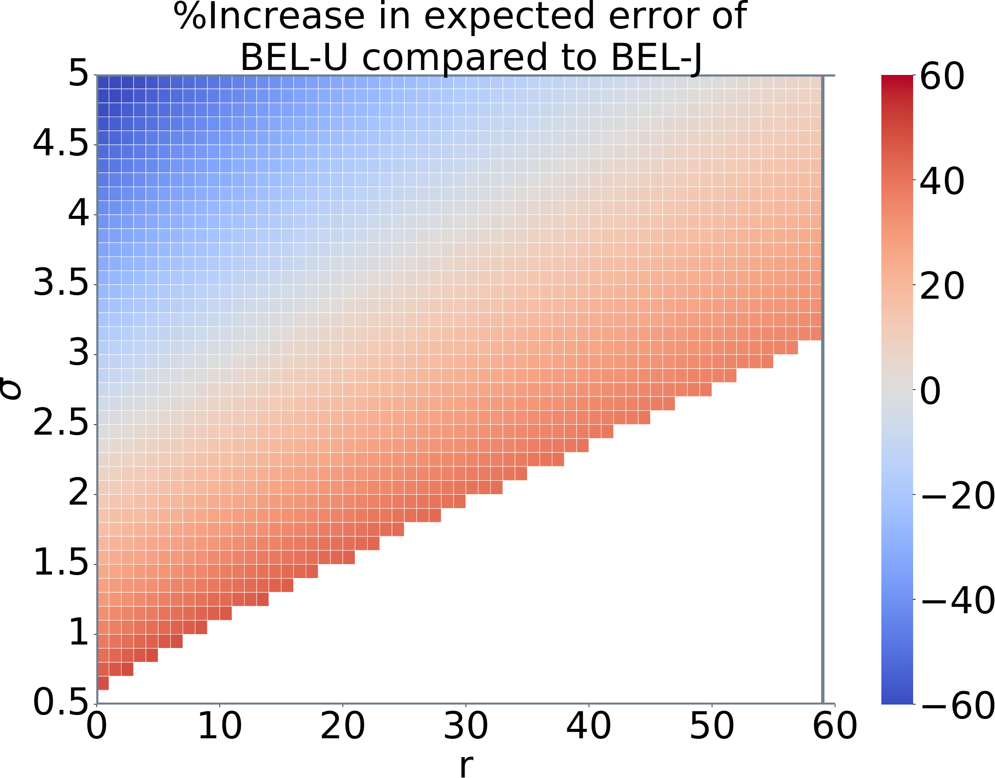
Based on the above analysis, we compare the expected absolute errors of BEL-U and BEL-J. Figure 3(c) represents the percentage increase in absolute error for BEL-U compared to BEL-J for valid values of standard deviation $\sigma$ ( $y-$ axis) and scaling factor $r$ ( $x-$ axis) as used in Equation 3 and 4. Here, BEL-J has a lower error in the red-colored region (%increase $>0$ ), whereas BEL-U has a lower error in the blue-colored region (%increase $<0$ ). The figure shows that whether BEL-J or BEL-U has lower error depends upon the values of $\sigma$ and $r$ . This suggests that the best $\{\mathcal{E},\mathcal{D}\}$ function will depend upon the classifier error probability distribution. The classifier error distribution in turn may depend upon the task, dataset, label distribution, network architecture, and optimization approach. Derivation of expected error for BEL-U and BEL-J and classifiers’ empirical error probability distributions for different architectures, datasets, and encodings are provided in Appendix B to C.

3.2 Design of Encoding Functions

Based on the above analysis and further empirical observation we identify three principles for selecting BEL codes for regression so as to minimize error. First, individual classifiers should require fewer bit transitions as this makes them easier to train. Second, a desirable property for a BEL encoding function is that the hamming distance between two codes (number of bits that differ) should be proportional to the difference between the target values they encode. However, hamming distance weighs all bit changes equally. Thus, hamming distance based code design provides equal error protection capability to all bits (Wu 2018; Xie et al. 2002) and does not account for which classifiers are more likely to mispredict for a given input. This matters because the misclassification probability of BEL classifiers is not uniform, but rather increases the closer the target value of an input is to a bit transition (e.g., Figure 3(a) and 3(b)). These observations yield a third important consideration: For a given target value classifiers closer to a bit transition are more likely to incur an error.

The principles above highlight a tradeoff between classification error probability and error-correction properties when selecting BEL codes. To evaluate the trade-offs, we empirically evaluate encodings that, to greater or lesser extent, satisfy one or more of the principles while focusing on reducing the number of classifiers (bits) so as to avoid increasing model parameters. Development of algorithms that might systematically optimize encoding functions is left to future work. Specifically, we explore the following codes:

Unary code (U): Unary codes (Figure 2(b)) have only one bit transition per classifier and thus require $M=N-1$ bits to encode $N$ values. Unary codes satisfy the first two principles and prior work on ordinal regression by binary classification (Li & Lin 2006; Niu et al. 2016) uses similar codes.

Johnson code (J): The Johnson code sequence (Figure 2(c)) is based on Libaw-Craig code (Libaw & Craig 1953). We select this code as it has well-separated bit transitions and requires $M=\frac{N}{2}$ bits compared to $N$ required for unary code. This code exemplifies the impact of considering non-uniform classifier error probabilities (third principle). For example the hamming distance between $1$ and $8$ is just one. However, the bit transition for the differing bit, for classifier $b^{1}$ , is far from $1$ or $8$ . Assuming equal error probability distributions centered on each bit transition for each classifier (as in Equation 4), $b^{1}$ is less likely to mispredict than $b^{2}$ , $b^{3}$ or $b^{4}$ for inputs with target values near $1$ or $8$ .

Base+displacement based code (B1JDJ/B2JDJ): We further reduce the number of bits using a base+displacement-based representation. In this representation, a value is represented in base-k using a base-term b and displacement d via b * k + d. b and d are represented using Johnson codes. Further, to improve the distance between two remote codes, we adapt reflected binary codes for term d (Gray 1953). We evaluate base-2 (B1JDJ - Figure 2(e)) and base-4 codes (B2JDJ - Figure 2(f)).

Binary coded hex - Johnson code (HEXJ): In HEXJ (Figure 2(g)), each digit (0-F) of the hexadecimal representation of a number is converted to an 8-bit binary code using Johnson code. For example, for the decimal number 47 (i.e., 2F in hex), HEXJ(47) = Concetanate(Johnson(2), Johnson(F)). A 16-bit HEXJ code can represent numbers in the range of 00 to FF (a total of 256). The number of bits increases sublinearly with the number of quantization levels for HEXJ, making it suitable for regression problems with many quantization levels.

Hadamard code (HAD): Hadamard codes (Bose & Shrikhande 1959) are widely used as error-correcting codes and have been used for multiclass classification (Dietterich & Bakiri 1995; Verma & Swami 2019). They require $M=N$ bits to encode $N$ values. However, Hadamard codes violate all three BEL code selection principles: First, each classifier has many bit transitions. Second, as each code is equidistant (hamming distance of $\frac{M}{2}$ ), the difference between target values is ignored. Finally, they protect all bits equally so do not take advantage of non-uniform error probabilities. We verify empirically Hadamard codes are unsuitable for regression (Section A).

3.3 Design of Decoding Functions

We explore three decoding functions: custom decoding, correlation-based decoding, and expected correlation-based decoding. Custom decoding functions are specific to the encoding function, and are only evaluated for unary and Johnson codes. In contrast, correlation-based decoding, first explored in prior work studying ECOC for multiclass classification (Allwein et al. 2001), can be applied to all codes. For quantized labels in $\{1,2,...,N\}$ , we define a code matrix ${\bm{C}}$ of size $N\times M$ , where $M$ is the number of bits/classifiers used for the binary-encoded label. Each row ${\bm{C}}_{k,:}$ in this matrix represents the binary code for label $Q_{i}=k$ . For example, Figure 2(b) can be considered a code matrix, where the first row represents code for label $Q_{i}=1$ . Let $\hat{Z}_{i}\in\mathbb{R}^{M}$ denote the output logit values of the classifiers. For decoding, the row with the highest correlation with the output $\hat{Z}_{i}$ is selected as the decoded label. Here, real-valued output $\hat{Z}_{i}$ is used instead of output binary code $\hat{B}_{i}$ to find the correlation as it uses the confidence of a classifier to make a more accurate prediction. For target quantized labels $Q_{i}\in\{1,2,...,N\}$ , the decoding function is defined as:

\mathcal{D}^{\text{GEN}}(\hat{Z}_{i})=\argmaxB_{k\in\{1,2,...,N\}}\Big(\hat{Z}_{i}\cdot{\bm{C}}_{k,:}\Big)

(5)

However, $\mathcal{D}^{\text{GEN}}$ outputs a quantized prediction, introducing quantization error. To remedy this concern and demonstrate the potential of more sophisticated decoding rules, we propose and evaluate an expected correlation-based decoding function, which allows prediction of real-valued label $\hat{y}_{i}$ . For target labels $y_{i}\in[1,N]$ , the decoding function is defined as:

\mathcal{D}^{\text{GEN-EX}}(\hat{Z}_{i})=\sum_{k=1}^{N}k\sigma_{k},\text{where }\sigma_{k}=\frac{e^{\hat{Z}_{i}\cdot{\bm{C}}_{k,:}}}{\sum_{j=1}^{N}e^{\hat{Z}_{i}\cdot{\bm{C}}_{j,:}}}

(6)

Training loss functions:

A deep neural network with multiple output binary classifiers can be trained using the binary cross-entropy (BCE) loss $\mathcal{L}_{\text{BCE}}\big(\hat{Z_{i}},\mathcal{E}(Q_{i})\big)$ . However, this loss minimizes the mismatch between predicted and target code but does not directly minimize the error between the target and predicted values. Decoding functions $\mathcal{D}^{\text{GEN}}$ and $\mathcal{D}^{\text{GEN-EX}}$ can be used to calculate the loss and minimize the mismatch between decoded predictions and target values directly. Decoding function $\mathcal{D}^{\text{GEN}}$ finds the correlation between each row of the code matrix ( ${\bm{C}}_{k,:}$ ) and the output $\hat{Z}_{i}$ . ${\bm{C}}{}\hat{Z}_{i}$ gives the correlation vector, and the index with the highest correlation is used as the predicted label. In this case, cross-entropy loss $\mathcal{L}_{\text{CE}}\big({\bm{C}}{}\hat{Z}_{i},Q_{i}\big)$ can be used to train the network. Similarly, for decoding function $\mathcal{D}^{\text{GEN-EX}}$ , which predicts a continuous value, L1 or L2 loss $\mathcal{L}_{\text{L1/L2}}\big(\mathcal{D}^{\text{GEN-EX}}(\hat{Z}_{i}),y_{i}\big)$ can also be used for training. We evaluate multiple combinations of decoding and loss functions in Section 4.

3.4 Regression Network Architecture for BEL

(a) Direct regression

(b) Binary-encoded labels

Figure 4: Network architecture for direct and BEL regression; only the regressor architecture is modified, but the entire network is trained end to end.

P

is the number of dimensions of the regression network output.

A regression network typically consists of a feature extractor and regressor. The regressor consists of a fully connected layer between the feature extractor’s output (i.e., feature vector) and output logits for direct regression as shown in Figure 4(a). In BEL, the number of output logits is increased to the number of classifiers (bits) used. When $y\in\mathbb{R}^{P}$ , with $P>1$ , the required number of output logits— $P\times M$ assuming $M$ -bit BEL encoding per output dimension—can significantly increase the size of the regression layer. However, empirically, we find small feature vectors suffice as the output logits are highly correlated for the explored encoding functions. Adding a fully connected bottleneck layer to reduce feature vector size to $\theta$ reduces the number of parameters and provides a trade-off between the model size and accuracy. Figure 4(b) shows the modified network architecture for BEL.

4 Evaluation

Table 1: Benchmarks used for evaluation

Task	Feature Extractor	Specialized Approach	Dataset	Benchmark	Label range/ Quantization levels	$\theta$
Landmark-free 2D head pose estimation	ResNet50	Regression+classification (Ruiz et al. 2018)	BIWI	HPE1	-100-100/200	10
			300LP/AFLW2000	HPE2	-100-100/200	10
	RAFANet	Direct regression (Behera et al. 2021)	BIWI	HPE3	-180-180/360	50
			300LP/AFLW2000	HPE4	-180-180/360	50
Facial Landmark Detection	HRNetV2-W18	Heatmap regression (Wang et al. 2020; Xu et al. 2020)	COFW	FLD1	0-256/256	10
			300W	FLD2	0-256/256	10
			WFLW	FLD3	0-256/256	10
			AFLW	FLD4	0-256/256	30
Age estimation	ResNet50 /ResNet34	Ordinal regression (Cao et al. 2020)	MORPH-II	AE1	0-64/64	10
			AFAD	AE2	0-32/32	10
End-to-end autonomous driving	PilotNet	Direct regression (Bojarski et al. 2017)	PilotNet	PN	0-670/670	10

Table 1 summarizes the tasks, datasets, and network architectures used for the evaluation of BEL. These tasks are commonly used for evaluation of regression approaches by prior works due to the complexity of problem and network architectures (Díaz & Marathe 2019). Landmark-free 2D head pose estimation (HPE) aims to find a human head’s pose in terms of three angles: yaw, pitch, and roll from a 2D image without landmarks. Facial landmark detection (FLD) is a problem of detecting the $(x,y)$ coordinates of keypoints in a given face image. Age estimation aims to predict the age of a person from an image. In end-to-end autonomous driving, the steering wheel’s next angle is predicted from an image of the road. Normalized Mean Error (NME) and Mean Absolute Error (MAE) with respect to raw real-valued labels are used as the evaluation metric for FLD and the rest, respectively.

We also evaluate direct regression and multiclass classification as baseline regression approaches. For direct regression, L1 or L2 loss functions are used. Label values are scaled to reduce the range of labels. The loss function and the scaling factors are set using hyperparameter tuning. In the multiclass classification-based regression, the target values are quantized and converted to a class. The network is trained using cross-entropy loss in this case. In our evaluation, the entire network (i.e., feature extractor and regressor) are trained end-to-end for direct regression, multiclass classification, and BEL. The feature extractor, data augmentation, evaluation protocols, and the number of training iterations are kept uniform across different methods for each benchmark. We report average of five training runs and error margin of $95\%$ confidence interval. Details on datasets, training parameters, related work for specific tasks, and other evaluation metrics are provided in Appendix C.

Figure 5: Error (MAE or NME) for different encoding, decoding, and loss functions for BEL. D1-D5 represents different combinations of decoding and loss functions: D1 (BCE loss with BEL-U/BEL-J/GEN decoding for U/J/others), D2 (CE/GEN-EX), D3 (CE/GEN), D4 (L1 or L2/GEN-EX), and D5 (BCE/GEN-EX).

BEL introduces several design parameters for regression by binary classification. We evaluate different encoding ( $\mathcal{E}$ ), decoding ( $\mathcal{D}$ ), and training loss ( $\mathcal{L}$ ) functions for BEL across all the benchmarks and study the extent and nature of the impact of these design parameters on accuracy.

Encoding function ( $\mathcal{E}$ ):

Figure 5 plots error (MAE or NME) using different encodings. We do not show results for Hadamard codes here as it results in significantly higher error than other encodings (Appendix A). On average, Hadamard codes result in $\sim 60\%$ higher error than J encoding, which shows that these codes are unsuitable for regression. The results show the encoding function significantly affects the accuracy and the best-performing encoding function varies across tasks, datasets, and network architectures (e.g., HPE1 and HPE3 are trained on the same dataset and different architecture). In Section 3.1 we observed that which encoding/decoding functions result in lower error depends upon the classifiers’ error distribution. For decoding functions used for the comparison in Section 3.1, J does better than U for HPE3, FLD1, and AE1; we attribute this to misclassification errors occurring more frequently near bit transitions based on the analytical study.

The encoding function impacts the number of classifiers and the complexity of the function to be learned by a classifier. We observe a trade-off between these two parameters. For some benchmarks, the availability of sufficient training data and network capacity facilitates the learning of complex classifiers such as B2JDJ. In such a case, a reduced number of classifiers compared to U, J, or B1JDJ codes results in a lower error. We provide empirical results for the same in Appendix A.

Decoding ( $\mathcal{D}$ ) and training loss ( $\mathcal{L}$ ) functions:

We explore three decoding and three training loss functions (Section 3.3). However, not all the combinations of decoding and loss functions ( $\mathcal{D}$ / $\mathcal{L}$ ) perform well. For example, CE, L1, or L2 losses do not use decodings $\mathcal{D}^{\text{BEL-J}}$ or $\mathcal{D}^{\text{BEL-U}}$ . Therefore, optimizing the network for these losses does not directly minimize the absolute error between targets and decoded predictions. We present results for five out of nine $\mathcal{D}$ / $\mathcal{L}$ combinations. Figure 5 compares error (MAE or NME) achieved by different $\mathcal{D}$ / $\mathcal{L}$ combinations and highlights the range of error variations. $\mathcal{D}^{\text{GEN-EX}}$ results in the lowest error for the majority of the benchmarks as it reduces quantization error and also utilizes the output logit confidence values. $\mathcal{D}^{\text{GEN-EX}}$ consistently perform better than $\mathcal{D}^{\text{GEN}}$ function that has been used for multiclass classification by prior works (Allwein et al. 2001). The use of CE or L1/L2 loss results in a lower error with $\mathcal{D}^{\text{GEN-EX}}$ for most benchmarks as the training loss function directly minimizes the error between targets and decoded predictions.

Comparison of BEL with regression approaches:

Table 2: Comparison of BEL with different regression approaches. “Specialized approach” described in Table 1

	Error (MAE or NME) / Model size
Approach	HPE1	HPE2	HPE3	HPE4
Specialized approach	-	-	3.40 / 69.8M	4.14 / 69.8M
Direct regression	4.76 $\pm$ 0.35 / 23.5M	5.65 $\pm$ 0.13 / 23.5M	3.40 $\pm$ 0.26 / 69.8M	4.14 $\pm$ 0.12 / 69.8M
Multiclass classification	4.49 $\pm$ 0.24 / 24.2M	5.31 $\pm$ 0.05 / 24.8M	4.54 $\pm$ 0.04 / 72.0M	5.14 $\pm$ 0.08 / 72.0M
BEL	3.56 $\pm$ 0.01 / 23.6M	4.77 $\pm$ 0.05 / 23.6M	3.30 $\pm$ 0.04 / 69.8M	3.90 $\pm$ 0.03 / 69.8M
BEL $\mathcal{E}/\mathcal{D}/\mathcal{L}$ functions	U/GEN-EX/L2	U/GEN-EX/BCE	B1JDJ/GEN-EX/BCE	U/GEN-EX/BCE

Approach	FLD1	FLD2	FLD3	FLD4
Specialized approach	3.45 / 9.6M	3.32 / 9.6M	4.32 / 9.6M	1.57 / 9.6M
Direct regression	3.60 $\pm$ 0.02 / 10.2M	3.54 $\pm$ 0.03 / 10.2M	4.64 $\pm$ 0.03 / 10.2M	1.51 $\pm$ 0.01 / 10.2M
Multiclass classification	3.58 $\pm$ 0.03 / 25.4M	3.51 $\pm$ 0.02 / 45.2M	4.50 $\pm$ 0.01 / 61.3M	1.56 $\pm$ 0.01 / 20.1M
BEL	3.34 $\pm$ 0.02 / 10.6M	3.40 $\pm$ 0.02 / 11.2M	4.36 $\pm$ 0.02 / 11.7M	1.47 $\pm$ 0.00 / 10.8M
BEL $\mathcal{E}/\mathcal{D}/\mathcal{L}$ functions	HEXJ/GEN-EX/CE	U/GEN-EX/CE	B1JDJ/GEN-EX/CE	B1JDJ/GEN-EX/CE

Approach	AE1	AE2	PN
Specialized approach	2.49 / 21.3M	3.47 / 21.3M	4.24 / 1.8M
Direct regression	2.44 $\pm$ 0.01 / 23.1M	3.21 $\pm$ 0.02 / 23.1M	4.24 $\pm$ 0.45 / 1.8M
Multiclass classification	2.75 $\pm$ 0.03 / 23.1M	3.38 $\pm$ 0.05 / 23.1M	5.54 $\pm$ 0.00 / 1.9M
BEL	2.27 $\pm$ 0.01 / 23.1M	3.11 $\pm$ 0.00 / 23.1M	3.11 $\pm$ 0.01 / 1.8M
BEL $\mathcal{E}/\mathcal{D}/\mathcal{L}$ functions	J/BEL-J/BCE	B1JDJ/GEN-EX/L1	J/GEN/CE

Table 2 compares BEL with other approaches for different benchmarks (Table 1). We explore and evaluate multiple combinations of encoding ( $\mathcal{E}$ ), decoding ( $\mathcal{D}$ ), and loss ( $\mathcal{L}$ ) functions for BEL in this work. In these experiments $20\%$ of the training set is used as validation set and the validation error is used to choose the best BEL approach. An ablation study for using more fully connected layers for direct regression and multiclass classification is in Appendix A. BEL results in lower error than direct regression and multiclass classification and even outperforms task-specific regression approaches for several benchmarks.

The results show no single combination of encoding/decoding/loss functions evaluated was best for all benchmarks but also demonstrate BEL improves accuracy across a range of regression problems.

5 Conclusion

This work proposes binary-encoded labels (BEL) to pose regression as binary classification. We propose a taxonomy identifying the key design aspects for regression by binary classification and demonstrate the impact of classification error and encoding/decoding functions on the expected label error. Different encoding, decoding, and loss functions are explored to evaluate our approach using four complex regression tasks. BEL results in an average $9.9\%$ , $15.5\%$ , and $7.2\%$ lower error than direct regression, multiclass classification, and task-specific regression approaches, respectively. BEL improves accuracy over state-of-the-art approaches for head pose estimation (BIWI, AFLW2000), facial landmark detection (COFW), age estimation (AFAD), and end-to-end autonomous driving (PilotNet). Our analysis and empirical evaluation in this work demonstrate the potential of the vast design space of BEL for regression problems and the importance of finding suitable design parameters for a given task. The best performing encoding/decoding function pair may be task, dataset, and network specific. A possibility this suggests, which we leave to future work, is that it may be beneficial to develop automated approaches for optimizing these functions.

6 Acknowledgements

This research has been funded in part by the National Sciences and Engineering Research Council of Canada (NSERC) Strategic Project Grant. Tor M. Aamodt serves as a consultant for Huawei Technologies Canada Co. Ltd. and Intel Corp. Deval Shah is partly funded by the Four Year Doctoral Fellowship (4YF) provided by the University of British Columbia.

Reproducibility:

We have provided a detailed discussion about training hyperparameters, experimental setup, and modifications made in publicly available network architectures in Appendix D.1-D.4 for all benchmarks. Code is available at https://github.com/ubc-aamodt-group/BEL_regression. We have provided the training and inference code with trained models.

Code of Ethics

Some of the major applications of regression problems are artificial intelligence and autonomous machines, and regression improvement can accelerate the development of autonomous systems. However, depending upon the use, autonomous systems can have some negative societal impacts, such as job loss in some sectors and ethical concerns.

References

fsa (2019) Fsa-net: Learning fine-grained structure aggregation for head pose estimation from a single image. Proceedings of the IEEE Computer Society Conference on Computer Vision and Pattern Recognition, 2019-June:1087–1096, 2019.
Allwein et al. (2001) Erin L. Allwein, Robert E. Schapire, and Yoram Singer. Reducing multiclass to binary: A unifying approach for margin classifiers. J. Mach. Learn. Res., 1:113–141, September 2001. doi: 10.1162/15324430152733133.
Behera et al. (2021) Ardhendu Behera, Zachary Wharton, Pradeep Hewage, and Swagat Kumar. Rotation axis focused attention network (rafa-net) for estimating head pose. In Computer Vision – ACCV 2020, 2021.
Berg et al. (2021) Axel Berg, Magnus Oskarsson, and Mark O’Connor. Deep ordinal regression with label diversity. In 2020 25th International Conference on Pattern Recognition (ICPR), pp. 2740–2747. IEEE, 2021.
Bojarski et al. (2016) Mariusz Bojarski, Davide Del Testa, Daniel Dworakowski, Bernhard Firner, Beat Flepp, Prasoon Goyal, Lawrence D. Jackel, Mathew Monfort, Urs Muller, Jiakai Zhang, Xin Zhang, Jake Zhao, and Karol Zieba. End to End Learning for Self-Driving Cars. arXiv:1604.07316, 2016.
Bojarski et al. (2017) Mariusz Bojarski, Philip Yeres, Anna Choromanaska, Krzysztof Choromanski, Bernhard Firner, Lawrence Jackel, and Urs Muller. Explaining how a deep neural network trained with end-to-end learning steers a car. arXiv:1704.07911, 2017.
Bose & Shrikhande (1959) R.C. Bose and S.S. Shrikhande. A note on a result in the theory of code construction. Information and Control, 2(2):183–194, 1959. doi: https://doi.org/10.1016/S0019-9958(59)90376-6.
Bulat & Tzimiropoulos (2016) Adrian Bulat and Georgios Tzimiropoulos. Human Pose Estimation via Convolutional Part Heatmap Regression. In Bastian Leibe, Jiri Matas, Nicu Sebe, and Max Welling (eds.), Computer Vision – ECCV 2016, pp. 717–732, 2016.
Burgos-Artizzu et al. (2013) Xavier Burgos-Artizzu, Pietro Perona, and Piotr Dollár. Robust Face Landmark Estimation under Occlusion. In Proceedings of the IEEE International Conference on Computer Vision, pp. 1513–1520, 12 2013. doi: 10.1109/ICCV.2013.191.
Cao et al. (2020) Wenzhi Cao, Vahid Mirjalili, and Sebastian Raschka. Rank consistent ordinal regression for neural networks with application to age estimation. Pattern Recognition Letters, 140:325–331, 2020. doi: https://doi.org/10.1016/j.patrec.2020.11.008.
Cardoso & Pinto da Costa (2007) Jaime S. Cardoso and Joaquim F. Pinto da Costa. Learning to Classify Ordinal Data: The Data Replication Method. Journal of Machine Learning Research, 8:1393–1429, 2007.
(12) Sully Chen. Driving-datasets. https://github.com/SullyChen/driving-datasets.
Chu & Keerthi (2005) Wei Chu and S. Sathiya Keerthi. New approaches to support vector ordinal regression. In Proceedings of the 22nd International Conference on Machine Learning, ICML ’05, pp. 145–152, 2005.
Cissé et al. (2012) M. Cissé, T. Artières, and Patrick Gallinari. Learning Compact Class Codes for Fast Inference in Large Multi Class Classification. In Peter A. Flach, Tijl De Bie, and Nello Cristianini (eds.), Machine Learning and Knowledge Discovery in Databases, pp. 506–520. Springer Berlin Heidelberg, 2012.
Crammer & Singer (2001) Koby Crammer and Yoram Singer. Pranking with Ranking. In Proceedings of the 14th International Conference on Neural Information Processing Systems: Natural and Synthetic, NIPS’01, pp. 641–647. MIT Press, 2001.
Dietterich & Bakiri (1995) T. G. Dietterich and G. Bakiri. Solving Multiclass Learning Problems via Error-Correcting Output Codes. Journal of Artificial Intelligence Research, 2:263–286, 1995. doi: 10.1613/jair.105.
Dong et al. (2018) Xuanyi Dong, Yan Yan, Wanli Ouyang, and Yi Yang. Style Aggregated Network for Facial Landmark Detection. In Proceedings of the IEEE Conference on Computer Vision and Pattern Recognition (CVPR), pp. 379–388, 2018.
Díaz & Marathe (2019) Raúl Díaz and Amit Marathe. Soft labels for ordinal regression. In 2019 IEEE/CVF Conference on Computer Vision and Pattern Recognition (CVPR), 2019. doi: 10.1109/CVPR.2019.00487.
Evron et al. (2018) Itay Evron, Edward Moroshko, and Koby Crammer. Efficient Loss-Based Decoding on Graphs for Extreme Classification. In Proceedings of the 32nd International Conference on Neural Information Processing Systems, NIPS’18, pp. 7233–7244, 2018.
Fanelli et al. (2013) Gabriele Fanelli, Matthias Dantone, Juergen Gall, Andrea Fossati, and Luc Gool. Random forests for real time 3d face analysis. International Journal of Computer Vision, 101(3):437–458, February 2013.
Fu et al. (2018) Huan Fu, Mingming Gong, Chaohui Wang, Kayhan Batmanghelich, and Dacheng Tao. Deep Ordinal Regression Network for Monocular Depth Estimation. Proceedings of the IEEE Computer Society Conference on Computer Vision and Pattern Recognition, pp. 2002–2011, 2018.
Gao et al. (2018) Bin-Bin Gao, Hong-Yu Zhou, Jianxin Wu, and Xin Geng. Age estimation using expectation of label distribution learning. In Proceedings of the Twenty-Seventh International Joint Conference on Artificial Intelligence, IJCAI-18, pp. 712–718, 7 2018. doi: 10.24963/ijcai.2018/99.
Gray (1953) Frank Gray. Pulse code communication, 1953.
Hsu et al. (2019) Heng-Wei Hsu, Tung-Yu Wu, Sheng Wan, Wing Hung Wong, and Chen-Yi Lee. Quatnet: Quaternion-based head pose estimation with multiregression loss. IEEE Transactions on Multimedia, 21(4):1035–1046, 2019. doi: 10.1109/TMM.2018.2866770.
Kowalski et al. (2017) Marek Kowalski, Jacek Naruniec, and Tomasz Trzcinski. Deep alignment network: A convolutional neural network for robust face alignment. In IEEE Conference on Computer Vision and Pattern Recognition Workshops, pp. 2034–2043, 2017. doi: 10.1109/CVPRW.2017.254.
Kumar et al. (2020) Abhinav Kumar, Tim K. Marks, Wenxuan Mou, Ye Wang, Michael Jones, Anoop Cherian, Toshiaki Koike-Akino, Xiaoming Liu, and Chen Feng. LUVLi face alignment: Estimating Landmarks’ location, uncertainty, and visibility likelihood. Proceedings of the IEEE Computer Society Conference on Computer Vision and Pattern Recognition, 2020. doi: 10.1109/CVPR42600.2020.00826.
Köstinger et al. (2011) M. Köstinger, P. Wohlhart, P. M. Roth, and H. Bischof. Annotated Facial Landmarks in the Wild: A large-scale, real-world database for facial landmark localization. In 2011 IEEE International Conference on Computer Vision Workshops (ICCV Workshops), pp. 2144–2151, 2011.
Li & Lin (2006) Ling Li and Hsuan-Tien Lin. Ordinal regression by extended binary classification. In Proceedings of the 19th International Conference on Neural Information Processing Systems, pp. 865–872, 2006.
Libaw & Craig (1953) William Libaw and Leonard Craig. A photoelectric decimal-coded shaft digitizer. Electronic Computers, Transactions of the I.R.E. Professional Group on, EC-2:1 – 4, 10 1953.
Lv et al. (2017) J. Lv, X. Shao, J. Xing, C. Cheng, and X. Zhou. A deep regression architecture with two-stage re-initialization for high performance facial landmark detection. In 2017 IEEE Conference on Computer Vision and Pattern Recognition (CVPR), pp. 3691–3700, 2017. doi: 10.1109/CVPR.2017.393.
Miao et al. (2018) X. Miao, X. Zhen, X. Liu, C. Deng, V. Athitsos, and H. Huang. Direct shape regression networks for end-to-end face alignment. In 2018 IEEE/CVF Conference on Computer Vision and Pattern Recognition, pp. 5040–5049, 2018.
Mukherjee & Robertson (2015) S. S. Mukherjee and N. M. Robertson. Deep head pose: Gaze-direction estimation in multimodal video. IEEE Transactions on Multimedia, 17(11):2094–2107, 2015.
Niu et al. (2016) Zhenxing Niu, Mo Zhou, Le Wang, Xinbo Gao, and Gang Hua. Ordinal regression with multiple output CNN for age estimation. Proceedings of the IEEE Computer Society Conference on Computer Vision and Pattern Recognition, 2016.
Pan et al. (2018) Hongyu Pan, Hu Han, Shiguang Shan, and Xilin Chen. Mean-variance loss for deep age estimation from a face. In 2018 IEEE/CVF Conference on Computer Vision and Pattern Recognition, pp. 5285–5294, 2018. doi: 10.1109/CVPR.2018.00554.
Raschka (2018) Sebastian Raschka. MLxtend: Providing machine learning and data science utilities and extensions to Python’s scientific computing stack. Journal of Open Source Software, 3(24):638, April 2018. doi: 10.21105/joss.00638.
Ricanek & Tesafaye (2006) K. Ricanek and T. Tesafaye. Morph: a longitudinal image database of normal adult age-progression. In 7th International Conference on Automatic Face and Gesture Recognition (FGR06), pp. 341–345, 2006. doi: 10.1109/FGR.2006.78.
Ruiz et al. (2018) Nataniel Ruiz, Eunji Chong, and James M. Rehg. Fine-grained head pose estimation without keypoints. In The IEEE Conference on Computer Vision and Pattern Recognition (CVPR) Workshops, June 2018.
Sagonas et al. (2013) C. Sagonas, G. Tzimiropoulos, S. Zafeiriou, and M. Pantic. 300 faces in-the-wild challenge: The first facial landmark localization challenge. In 2013 IEEE International Conference on Computer Vision Workshops, pp. 397–403, 2013.
Shizhan Zhu et al. (2015) Shizhan Zhu, Cheng Li, C. C. Loy, and X. Tang. Face alignment by coarse-to-fine shape searching. In 2015 IEEE Conference on Computer Vision and Pattern Recognition (CVPR), pp. 4998–5006, 2015.
Song et al. (2021) Yang Song, Qiyu Kang, and Wee Peng Tay. Error-Correcting Output Codes with Ensemble Diversity for Robust Learning in Neural Networks. AAAI, 2021.
Sun et al. (2013) Y. Sun, X. Wang, and X. Tang. Deep convolutional network cascade for facial point detection. In 2013 IEEE Conference on Computer Vision and Pattern Recognition, pp. 3476–3483, 2013. doi: 10.1109/CVPR.2013.446.
Tzimiropoulos (2015) G. Tzimiropoulos. Project-out cascaded regression with an application to face alignment. In 2015 IEEE Conference on Computer Vision and Pattern Recognition (CVPR), pp. 3659–3667, 2015.
Verma & Swami (2019) Gunjan Verma and Ananthram Swami. Error correcting output codes improve probability estimation and adversarial robustness of deep neural networks. Advances in Neural Information Processing Systems, 32(NeurIPS), 2019.
Wang et al. (2020) Jingdong Wang, Ke Sun, Tianheng Cheng, Borui Jiang, Chaorui Deng, Yang Zhao, Dong Liu, Yadong Mu, Mingkui Tan, Xinggang Wang, Wenyu Liu, and Bin Xiao. Deep high-resolution representation learning for visual recognition. IEEE transactions on pattern analysis and machine intelligence, PP, April 2020.
Wang et al. (2019) Xinyao Wang, Liefeng Bo, and Fuxin Li. Adaptive wing loss for robust face alignment via heatmap regression. In 2019 IEEE International Conference on Computer Vision (ICCV), pp. 6970–6980, 2019. doi: 10.1109/ICCV.2019.00707.
Wu (2018) Chai Wah Wu. Designing communication systems via iterative improvement: error correction coding with bayes decoder and codebook optimized for source symbol error. ArXiv:1805.07429, 2018.
Wu & Yang (2017) W. Wu and S. Yang. Leveraging intra and inter-dataset variations for robust face alignment. In 2017 IEEE Conference on Computer Vision and Pattern Recognition Workshops (CVPRW), pp. 2096–2105, 2017.
Wu et al. (2018) W. Wu, Chen Qian, S. Yang, Q. Wang, Y. Cai, and Qiang Zhou. Look at boundary: A boundary-aware face alignment algorithm. 2018 IEEE/CVF Conference on Computer Vision and Pattern Recognition, pp. 2129–2138, 2018.
Xie et al. (2002) Ley Xie, Huifang Chen, Peiliang Qiu, and Ming Zhang. The modified hamming bound for unequal error protection codes. In IEEE 2002 International Conference on Communications, Circuits and Systems and West Sino Expositions, 2002. doi: 10.1109/ICCCAS.2002.1180579.
Xiong & De la Torre (2013) X. Xiong and F. De la Torre. Supervised descent method and its applications to face alignment. In 2013 IEEE Conference on Computer Vision and Pattern Recognition, pp. 532–539, 2013.
Xu et al. (2020) Zixuan Xu, Banghuai Li, Miao Geng, Ye Yuan, and Gang Yu. Anchorface: An anchor-based facial landmark detector across large poses. ArXiv:2007.03221, 2020.
Yang et al. (2018) Tsun-Yi Yang, Yi-Hsuan Huang, Yen-Yu Lin, Pi-Cheng Hsiu, and Yung-Yu Chuang. Ssr-net: A compact soft stagewise regression network for age estimation. In Proceedings of the 27th International Joint Conference on Artificial Intelligence, IJCAI’18, pp. 1078–1084. AAAI Press, 2018. ISBN 9780999241127.
Zhang et al. (2014) Jie Zhang, Shiguang Shan, Meina Kan, and Xilin Chen. Coarse-to-fine auto-encoder networks (cfan) for real-time face alignment. In Computer Vision – ECCV 2014, pp. 1–16, 2014.
Zhu et al. (2016) S. Zhu, C. Li, C. C. Loy, and X. Tang. Unconstrained face alignment via cascaded compositional learning. In 2016 IEEE Conference on Computer Vision and Pattern Recognition (CVPR), pp. 3409–3417, 2016. doi: 10.1109/CVPR.2016.371.
Zhu et al. (2016) Xiangyu Zhu, Zhen Lei, Xiaoming Liu, Hailin Shi, and Stan Li. Face alignment across large poses: A 3d solution. In Proceedings of the IEEE Computer Society Conference on Computer Vision and Pattern Recognition, pp. 146–155, 06 2016.

Appendix A Ablation study

Impact of combination of encoding, decoding, and loss functions:

We propose multiple combinations of encoding, decoding, and loss functions that can be used with BEL. In Tables 3- 13, we show the effect of each combination of encoding, decoding, and loss function on the error of the model. Although general trends exist and some combinations perform consistently well across datasets, the optimal combination varies based on the dataset.

Table 3: Comparison of BEL design parameters on MAE for head pose estimation with BIWI dataset and ResNet50 feature extractor (HPE1).

		Encoding function
Decoding function	Loss function	U	J	B1JDJ	B2JDJ	HEXJ	HAD
BEL-J/BEL-U	BCE	3.38	3.65	-	-	-	-
GEN-EX	BCE	3.37	3.64	5.11	8.02	4.76	7.53
GEN	BCE	3.38	3.65	5.16	8.16	4.99	7.73
GEN-EX	CE	4.22	3.55	3.88	4.08	4.09	5.50
GEN	CE	4.25	3.62	3.93	4.06	4.39	5.48
GEN-EX	L2	3.56	3.93	3.66	3.59	5.99	4.21

Table 4: Comparison of BEL design parameters on MAE for head pose estimation with 300LP/AFLW2000 datasets and ResNet50 feature extractor (HPE2).

		Encoding function
Decoding function	Loss function	U	J	B1JDJ	B2JDJ	HEXJ	HAD
BEL-J/BEL-U	BCE	4.78	4.84	-	-	-	-
GEN-EX	BCE	4.77	4.84	5.43	5.09	4.94	7.84
GEN	BCE	4.78	4.87	5.11	5.05	5.15	8.54
GEN-EX	CE	4.93	5.04	5.04	4.97	4.79	5.64
GEN	CE	5.07	5.17	5.13	5.10	4.99	5.62
GEN-EX	L2	5.05	5.18	5.19	5.09	5.17	5.07

Table 5: Comparison of BEL design parameters on MAE for head pose estimation with BIWI dataset and RAFA-Net feature extractor (HPE3).

		Encoding function
Decoding function	Loss function	U	J	B1JDJ	B2JDJ	HEXJ	HAD
BEL-J/BEL-U	BCE	3.47	3.16	-	-	-	-
GEN-EX	BCE	3.46	3.12	3.30	3.35	3.80	5.75
GEN	BCE	3.49	3.14	3.62	3.78	4.44	5.83
GEN-EX	CE	3.82	3.91	3.52	3.49	3.98	3.98
GEN	CE	3.92	4.09	3.62	3.65	4.35	4.28
GEN-EX	L2	3.72	3.60	4.31	4.29	6.61	18.69

Table 6: Comparison of BEL design parameters on MAE for head pose estimation with 300LP/AFLW2000 datasets and RAFA-Net feature extractor (HPE4).

		Encoding function
Decoding function	Loss function	U	J	B1JDJ	B2JDJ	HEXJ	HAD
BEL-J/BEL-U	BCE	3.94	4.00	-	-	-	-
GEN-EX	BCE	3.90	3.93	4.19	4.12	4.39	9.17
GEN	BCE	3.93	3.94	4.21	4.25	4.53	9.21
GEN-EX	CE	4.55	4.62	4.34	4.53	4.45	5.12
GEN	CE	4.68	4.75	4.46	4.61	4.63	5.29
GEN-EX	L2	4.45	5.87	5.11	9.34	10.43	17.89

Table 7: Comparison of BEL design parameters on NME for facial landmark detection with COFW dataset and HRNetV2-W18 feature extractor (FLD1).

		Encoding function
Decoding function	Loss function	U	J	B1JDJ	B2JDJ	HEXJ	HAD
BEL-J/BEL-U	BCE	3.47	3.45	-	-	-	-
GEN-EX	BCE	3.45	3.43	3.42	3.41	3.47	4.28
GEN	BCE	3.46	3.45	3.43	3.47	3.66	4.43
GEN-EX	CE	3.37	3.37	3.38	3.41	3.34	3.69
GEN	CE	3.44	3.44	3.44	3.49	3.57	3.69
GEN-EX	L1	3.44	3.41	3.45	3.47	3.41	4.52

Table 8: Comparison of BEL design parameters on NME for facial landmark detection with 300W dataset and HRNetV2-W18 feature extractor (FLD2).

		Encoding function
Decoding function	Loss function	U	J	B1JDJ	B2JDJ	HEXJ	HAD
BEL-J/BEL-U	BCE	3.5	3.49	-	-	-	-
GEN-EX	BCE	3.48	3.46	3.43	3.42	3.38	4.71
GEN	BCE	3.50	3.49	3.45	3.45	3.55	4.78
GEN-EX	CE	3.40	3.36	3.37	3.41	3.37	3.62
GEN	CE	3.50	3.45	3.45	3.51	3.59	3.65
GEN-EX	L1	3.41	3.39	3.49	3.67	3.43	4.04

Table 9: Comparison of BEL design parameters on NME for facial landmark detection with WFLW dataset and HRNetV2-W18 feature extractor (FLD3).

		Encoding function
Decoding function	Loss function	U	J	B1JDJ	B2JDJ	HEXJ	HAD
BEL-J/BEL-U	BCE	4.62	4.54	-	-	-	-
GEN-EX	BCE	4.6	4.51	4.43	4.38	4.37	7.18
GEN	BCE	4.62	4.53	4.44	4.42	4.55	7.14
GEN-EX	CE	4.36	4.34	4.36	4.33	4.34	5.15
GEN	CE	4.46	4.44	4.47	4.47	4.56	4.83
GEN-EX	L1	4.39	4.42	4.47	4.47	4.45	4.74

Table 10: Comparison of BEL design parameters on NME for facial landmark detection with AFLW dataset and HRNetV2-W18 feature extractor (FLD4).

		Encoding function
Decoding function	Loss function	U	J	B1JDJ	B2JDJ	HEXJ	HAD
BEL-J/BEL-U	BCE	1.51	1.52	-	-	-	-
GEN-EX	BCE	1.50	1.50	1.47	1.47	1.49	1.52
GEN	BCE	1.51	1.52	1.50	1.49	1.54	1.55
GEN-EX	CE	1.48	1.47	1.47	1.47	1.47	1.47
GEN	CE	1.52	1.51	1.51	1.51	1.52	1.52
GEN-EX	L1	1.47	1.47	1.48	1.48	1.48	1.59

Table 11: Comparison of BEL design parameters on MAE for age estimation with MORPH-II dataset and ResNet50 feature extractor (AE1).

		Encoding function
Decoding function	Loss function	U	J	B1JDJ	B2JDJ	HEXJ	HAD
BEL-J/BEL-U	BCE	2.32	2.27	-	-	-	-
GEN-EX	BCE	2.30	2.29	2.35	2.49	2.45	2.99
GEN	BCE	2.28	2.28	2.34	2.51	2.54	3.07
GEN-EX	CE	2.55	2.54	2.75	2.65	2.63	12.33
GEN	CE	2.60	2.58	2.61	2.66	2.61	3.10
GEN-EX	L1	2.30	2.30	2.32	2.30	2.32	2.29

Table 12: Comparison of BEL design parameters on MAE for age estimation with AFAD dataset and ResNet50 feature extractor (AE2).

		Encoding function
Decoding function	Loss function	U	J	B1JDJ	B2JDJ	HEXJ	HAD
BEL-J/BEL-U	BCE	3.13	3.15	-	-	-	-
GEN-EX	BCE	3.14	3.16	3.32	3.35	3.28	3.34
GEN	BCE	3.13	3.19	3.41	3.44	3.41	3.52
GEN-EX	CE	3.26	3.29	3.38	3.44	3.40	3.30
GEN	CE	3.36	3.34	3.42	3.47	3.40	3.45
GEN-EX	L1	3.13	3.12	3.11	3.12	3.13	3.13

Table 13: Comparison of BEL design parameters on MAE for end-to-end autonomous driving with PilotNet dataset and feature extractor (PN).

		Encoding function
Decoding function	Loss function	U	J	B1JDJ	B2JDJ	HEXJ	HAD
BEL-J/BEL-U	BCE	4.34	3.91	-	-	-	-
GEN-EX	BCE	4.57	4.20	4.83	4.96	5.29	10.12
GEN	BCE	4.37	3.95	3.51	3.61	4.01	10.00
GEN-EX	CE	4.30	4.16	4.99	5.87	5.39	87.17
GEN	CE	3.15	3.11	3.14	3.21	3.64	6.20
GEN-EX	L1	4.10	4.11	4.34	4.34	4.11	5.09

Impact of quantization and decoding functions:

As discussed in Section 3, a real-valued label is quantized to a discrete value in $\{1,2,...,N\}$ before applying the encoding function. In Table 14, we show the effect of increasing the number of quantization levels ( $N$ ) on the error for correlation-based decoding ( $\mathcal{D}^{\text{GEN}}$ , which returns a quantized prediction) and expected correlation-based decoding ( $\mathcal{D}^{\text{GEN-EX}}$ , which returns a continuous prediction). As shown in the table, there exists a tradeoff between reducing quantization error and using fewer classifiers. The error is lower for 128 quantization levels than it is for 256 as the improvement resulting from fewer binary classifiers is higher than the increase in quantization error. Moreover, the use of proposed decoding function $\mathcal{D}^{\text{GEN-EX}}$ for regression consistently results in lower error compared to $\mathcal{D}^{\text{GEN}}$ .

Table 14: Impact of the quantization and decoding functions on NME for facial landmark detection.

	COFW			300W
Quantization levels	64	128	256	64	128	256
$\mathcal{E}^{\text{BEL-U}}$ + $\mathcal{D}^{\text{GEN}}$	3.66	3.51	3.46	3.79	3.59	3.46
$\mathcal{E}^{\text{BEL-U}}$ + $\mathcal{D}^{\text{GEN-EX}}$	3.46	3.41	3.44	3.54	3.47	3.44
$\mathcal{E}^{\text{BEL-J}}$ + $\mathcal{D}^{\text{GEN}}$	3.65	3.49	3.43	3.76	3.58	3.46
$\mathcal{E}^{\text{BEL-J}}$ + $\mathcal{D}^{\text{GEN-EX}}$	3.45	3.40	3.42	3.52	3.45	3.43

Impact of the number of training samples on BEL:

As discussed in Section 4, the performance of different encoding functions varies depending on the availability of sufficient training data. In Table 15, we analyze the effect of the number of available training samples for both simple and complex encodings. We use the number of bit transitions as a measure of the complexity of a classifier. As the number of training samples decreases, simpler encodings (U and J) perform better than more complex encodings (B1JDJ, B2JDJ, and HEXJ). Using a more complex encoding reduces the number of classifiers; however, it increases each classifier’s complexity (i.e. the number of bit transitions) and thus performs poorly with less training data.

Table 15: Effect of training dataset size on optimal encoding function for facial landmark detection. BCE loss function and GEN-EX decoding function are used for the training and evaluation.

			Reduction in the number training samples
Encoding	#Classifiers/label	#bit transitions/classifier	0%	20%	40%	60%	80%	90%	95%
COFW (FLD1)
U	256	1	3.45	3.48	3.55	3.72	3.94	4.52	6.29
J	128	2	3.43	3.48	3.51	3.61	3.88	4.32	5.39
B1JDJ	65	4	3.42	3.44	3.52	3.60	4.11	4.50	5.68
B2JDJ	34	8	3.41	3.45	3.48	3.80	3.94	4.80	6.56
HEXJ	17	32	3.47	3.69	3.78	4.03	4.61	5.48	6.69
300W (FLD2)
U	256	1	3.48	3.55	3.58	3.64	3.89	4.26	5.66
J	128	2	3.46	3.56	3.52	3.58	3.79	4.04	4.58
B1JDJ	65	4	3.43	3.48	3.53	3.61	3.89	4.31	6.10
B2JDJ	34	8	3.42	3.47	3.51	3.54	3.88	4.50	5.80
HEXJ	17	32	3.38	3.64	3.73	3.97	4.41	5.38	6.60
WFLW (FLD3)
U	256	1	4.60	4.67	4.83	5.00	5.37	6.04	7.46
J	128	2	4.51	4.60	4.65	4.84	5.23	5.64	6.39
B1JDJ	65	4	4.43	4.44	4.52	4.66	5.08	5.90	8.39
B2JDJ	34	8	4.38	4.46	4.49	4.61	5.02	5.95	8.78
HEXJ	17	32	4.37	4.60	4.72	4.96	5.72	6.86	8.09
AFLW (FLD4)
U	256	1	1.50	1.53	1.53	1.56	1.61	1.68	1.83
J	128	2	1.50	1.51	1.52	1.54	1.60	1.68	1.79
B1JDJ	65	4	1.47	1.50	1.52	1.54	1.60	1.67	1.78
B2JDJ	34	8	1.47	1.50	1.50	1.52	1.57	1.64	1.73
HEXJ	17	32	1.49	1.54	1.54	1.55	1.59	1.71	1.89

Impact of reflected binary conversion:

As mentioned in Section 3, we use reflected binary to increase the distance between distant labels based on the design properties of suitable regression encodings we proposed. Table 16 shows the impact of using reflected binary conversion on error for facial landmark detection benchmarks. As shown in the table, the use of reflected binary significantly reduces the error.

Table 16: Effect of reflected binary conversion for B1JDJ encoding on facial landmark detection. Here, BCE loss and GEN-EX decoding functions are used.

	COFW	300W	WFLW	AFLW
B1JDJ	3.43	3.46	4.43	1.47
B1JDJ- w/o reflected binary	4.13	4.43	5.70	1.97

Use of binary heamaps:

Facial landmark detection approaches typically use heatmap regression. We also evaluate BEL-H-x, in which the real-valued heatmaps are converted to binary heatmaps with $8$ quantization levels. Table 17 shows the impact of using binary heatmaps on error for facial landmark detection benchmarks. For unary code, a $64\times 64$ real-valued heatmap of one facial landmark is converted to eight $64\times 64$ binary heatmaps, resulting in $32,768$ ( $8\times 64\times 64$ ) binary classifiers compared to $512$ for BEL-U. We believe that training a high number of binary classifiers results in high error for BEL-H-x.

Table 17: Comparison of BEL with heatmaps for facial landmark detection. Here, BCE loss and GEN-EX decoding functions are used.

	FLD1	FLD2	FLD3	FLD4
BEL-U	3.45	3.46	4.60	1.50
BEL-J	3.48	3.46	4.51	1.50
BEL-H-U	4.13	4.43	5.70	1.97
BEL-H-J	10.17	33.02	22.50	2.99

Hyperparameter $\theta$ :

As shown in Figure 4b, we introduce a feature vector of size $\theta$ before the output layer. Figure 6 compares the decrease in the error for different encodings and $\theta$ values. We observe that more complex encodings benefit more from an increase in the value of $\theta$ , while a lower value of $\theta$ can be used for simpler encodings.

Figure 6: Effect of

\theta

on error for different encodings on FLD1.

Impact of increasing the number of fully connected layers:

Table 18: Impact increasing number of fully connected layers in direct regression and multiclass classification on the error (MAE or NME).

Benchmark	Direct regression		Multiclass classification		BEL
Benchmark	1 FC layer	2 FC layers	1 FC layer	2 FC layers	2 FC layers
HPE1	4.76	5.19	4.49	4.82	3.37
HPE2	5.65	5.59	5.31	5.42	4.77
HPE3	3.40	3.54	4.45	4.54	3.12
HPE4	4.14	4.22	5.14	5.45	3.90
FLD1	3.60	3.63	3.58	3.56	3.34
FLD2	3.54	3.58	3.51	3.62	3.36
FLD3	4.64	4.63	4.50	4.64	4.33
FLD4	1.51	1.51	1.56	1.53	1.47
AE1	2.44	2.35	2.75	2.81	2.27
AE2	3.21	3.14	3.38	3.40	3.11
PN	4.24	4.33	4.56	5.74	3.11

For BEL, we propose to add a fully connected bottleneck layer in the regressor to reduce the feature vector size to $\theta$ and thus decrease the number of parameters in the regressor. We perform an ablation study to study the impact of this added fully connected layer on relative performance of direct regression, multiclass classification, and binary encoded labels. Table 18 provides the error (MAE or NME) for direct regression and multiclass classification with one or two fully connected layers after the feature extractor. Further, we evaluate BEL, direct regression, and multiclass classification for higher number of fully connected layers as shown in Table 19. We observe that increasing the number of fully connected layers in direct regression and multiclass classification does not improve the accuracy for most benchmarks (possibly due to overparameterization). BEL with two fully connected layers outperforms direct regression and multiclass classification in both cases. Furthermore, even for a higher number of fully connected layers in BEL, the suitability of an encoding function varies with the dataset, demonstrating the importance of BEL design space.

Table 19: Impact increasing number of fully connected layers in direct regression, multiclass classification, and BEL. GEN-EX decoding function and BCE loss function are used for BEL.

Benchmark	# FC layers (size of FC layers)	Direct regression	Multiclass classification	U	J	B1JDJ	B2JDJ	HEXJ
FLD1	1 (1024-x)	3.6	3.58	-	-	-	-	-
	2 (1024-30-x)	3.63	3.56	3.45	3.43	3.42	3.41	3.47
	3 (1024-30-10-x)	3.63	3.94	3.55	3.47	3.82	4.02	3.62
FLD2	1 (1024-x)	3.54	3.51	-	-	-	-	-
	2 (1024-10-x)	3.58	3.62	3.48	3.46	3.43	3.42	3.38
	3 (1024-30-10-x)	3.55	3.78	3.42	3.46	3.5	3.61	3.52

Training-validation set based evaluation:

Ideally, a validation set should be used for model selection. Hence we have reevaluated the benchmarks with a validation set to select the best design parameters and the best model (i.e., which model is the best over multiple epochs). Since datasets used in benchmarks do not provide separate validation datasets, we use $20\%$ of the training data as a validation set. Since earlier works use $100\%$ training data for the reported results and use test error for model selection, we have re-run specialized approaches (if possible), direct regression, and multiclass classification. It was not possible for us to re-run experiments for all specialized approaches due to resource constraints, and the comparison is conservative for many benchmarks.

Table 20 compares different regression approaches for this evaluation setup. Note that the additional results do not diminish the effectiveness of BEL and BEL outperforms direct regression and multiclass classification for all benchmarks and specialized approaches for several benchmarks.

Table 20: Comparison of BEL with different regression approaches. Specialized approaches for each benchmark are described in Table 1

	Error (MAE or NME) / Model size
Approach (% training set)	HPE1	HPE2	HPE3	HPE4
Specialized approach (100%)	-	-	3.40 / 69.8M	4.14 / 69.8M
Specialized approach (80%)	-	-	4.08 $\pm$ 0.11 / 69.8M	4.69 $\pm$ 0.02 / 69.8M
Direct regression (80%)	6.12 $\pm$ 0.02 / 23.5M	5.97 $\pm$ 0.09 / 23.5M	4.08 $\pm$ 0.11 / 69.8M	4.67+4.70 / 69.8M
Multiclass classification (80%)	5.38 $\pm$ 0.03 / 24.2M	5.60 $\pm$ 0.13 / 24.8M	5.58 $\pm$ 0.04 / 72.0M	5.86 $\pm$ 0.10 / 72.0M
BEL (80%)	3.91 $\pm$ 0.08 / 23.6M	4.91 $\pm$ 0.10 / 23.6M	3.50 $\pm$ 0.08 / 69.8M	3.99 $\pm$ 0.04 / 69.8M
BEL $\mathcal{E}/\mathcal{D}/\mathcal{L}$ functions	U/GEN-EX/L2	U/GEN-EX/BCE	B1JDJ/GEN-EX/BCE	U/GEN-EX/BCE

Approach (%training set)	FLD1	FLD2	FLD3	FLD4
Specialized approach (100%)	3.45 / 9.6M	3.32 / 9.6M	4.32 / 9.6M	1.57 / 9.6M
Direct regression (80%)	3.70 $\pm$ 0.04 / 10.2M	3.69 $\pm$ 0.06 / 10.2M	4.71 $\pm$ 0.02 / 10.2M	1.51 $\pm$ 0.01 / 10.2M
Multiclass classification (80%)	3.64 $\pm$ 0.02 / 25.4M	3.68 $\pm$ 0.02 / 45.2M	4.77 $\pm$ 0.02 / 61.3M	1.56 $\pm$ 0.01 / 20.1M
BEL (80%)	3.35 $\pm$ 0.02 / 10.6M	3.40 $\pm$ 0.03 / 11.2M	4.37 $\pm$ 0.01 / 11.7M	1.48 $\pm$ 0.01 / 10.8M
BEL $\mathcal{E}/\mathcal{D}/\mathcal{L}$ functions	HEXJ/GEN-EX/CE	U/GEN-EX/CE	B1JDJ/GEN-EX/CE	B1JDJ/GEN-EX/CE

Approach (% training set)	AE1	AE2	PN
Specialized approach (100%)	2.49 / 21.3M	3.47 / 21.3M	4.24 / 1.8M
Direct regression (80%)	2.45 $\pm$ 0.01 / 23.1M	3.34 $\pm$ 0.02 / 23.1M	4.56 $\pm$ 0.45 / 1.8M
Multiclass classification (80%)	2.85 $\pm$ 0.03 / 23.1M	3.47 $\pm$ 0.05 / 23.1M	6.37 $\pm$ 0.00 / 1.9M
BEL (80%)	2.36 $\pm$ 0.01 / 23.1M	3.20 $\pm$ 0.00 / 23.1M	3.49 $\pm$ 0.01 / 1.8M
BEL $\mathcal{E}/\mathcal{D}/\mathcal{L}$ functions	J/BEL-J/BCE	B1JDJ/GEN-EX/L1	J/GEN/CE

Appendix B Expected Error Derivation

This section explains the expected error equations used to compare BEL-U and BEL-J in Section 3. We first explain the encoding and decoding function used for BEL-U and derive the relation between the expected regression error and classification error for BEL-U. Then, we explain the encoding/decoding functions and expected error relation for BEL-J.

B.1 Preliminaries

Given a sample $i$ drawn from a dataset with minimum label $a$ and maximum label $b$ , let $y_{i}\in[a,b]$ represent the target label for that sample. Assuming uniform quantization, the range of target labels can be quantized using $q:[a,b]\to\{1,2,...,N\}$ through Equation 7.

q(y_{i})=(y_{i}-a)*\frac{N-1}{b-a}+1

(7)

We define the encoding function $\mathcal{E}:\{1,2,...,N-1\}\to\{0,1\}^{M}$ to convert a target quantized level $Q_{i}\in\{1,2,...,N-1\}$ to a binary code $B_{i}\in\{0,1\}^{M}$ . We further define the decoding function $\mathcal{D}:\{0,1\}^{M}\to[a,b]$ to convert the predicted binary code $\hat{B_{i}}$ to the predicted label $\hat{y_{i}}$ .

Although the decoding functions used in this analysis predict the quantized label and introduce quantization error, we do not include quantization error in the expected absolute error for our analysis as it is constant for both BEL-U and BEL-J. The expected value of absolute error between the target $y$ and predicted labels $\hat{y}$ is used for the analysis as typically mean absolute error is used as the evaluation metric in regression problems.

Let us denote the error probability of a binary classifier $C^{k}$ used to predict bit $k$ in a binary code $B_{i}=\mathcal{E}(n)$ as $e_{k}(n)$ , where $n$ is the target quantized label $Q_{i}$ . Then,

\begin{split}e_{k}(n)&=\EX(|\hat{b}_{i}^{k}-b_{i}^{k}|)\\ &=Pr(\hat{b}_{i}^{k}=F)\text{ for target label $Q_{i}=n$ and target binary code $B_{i}=\mathcal{E}(n)$}\end{split}

(8)

where $\hat{b}_{i}^{k}=T$ indicates a correct binary classification by classifier $C^{k}$ ( $\hat{b}_{i}^{k}==b_{i}^{k}$ ) for sample $i$ and $\hat{b}_{i}^{k}=F$ indicates an incorrect binary classification by classifier $C^{k}$ ( $\hat{b}_{i}^{k}\neq b_{i}^{k}$ ) for sample $i$ .

B.2 Expected Error for BEL-U

Encoding and decoding functions:

The encoding and decoding functions for BEL-U are defined as:

\mathcal{E}^{\text{BEL-U}}(Q_{i})=b_{i}^{1},b_{i}^{2},..,b_{i}^{N-2}\text{, where }b_{i}^{k}=\begin{cases}1,&k<Q_{i}\\ 0,&\text{Otherwise}\\ \end{cases}

(9)

\mathcal{D}^{\text{BEL-U}}(\hat{b}_{i}^{1},\hat{b}_{i}^{2},...,\hat{b}_{i}^{N-2})=\sum_{k=1}^{N-2}\hat{b}_{i}^{k}+1

(10)

Expected error:

For target quantized label $Q_{i}=n$ ( $n\in\{1,2,...,N-1\}$ ), ignoring the quantization error, the expected error between target $y_{i}$ and predicted label $\hat{y}_{i}$ can be derived as:

\begin{split}\EX(|\hat{y}_{i}^{\text{BEL-U}}-y_{i}|)&=\EX\Big(\Big|\sum_{k=1}^{N-2}\big(\hat{b}_{i}^{k}+1\big)-\sum_{k=1}^{N-2}\big(b_{i}^{k}+1\big)\Big|\Big)\\ &=\EX\Big(\Big|\sum_{k=1}^{N-2}(\hat{b}_{i}^{k}-b_{i}^{k})\Big|\Big)\\ &\leqslant\EX\Big(\sum_{k=1}^{N-2}|\hat{b}_{i}^{k}-b_{i}^{k}|\Big)\\ &=\sum_{k=1}^{N-2}\EX|\hat{b}_{i}^{k}-b_{i}^{k}|\\ &=\sum_{k=1}^{N-2}e_{k}(n)\text{ (using ~Equation~\ref{eq:err}) }\end{split}

(11)

For a uniform distribution of target labels in the range $[1,N-1]$ , the expected error can be derived as:

\EX(|\hat{y}^{\text{BEL-U}}-y|)\leqslant\frac{1}{N-1}\sum_{n=1}^{N-1}\sum_{k=1}^{N-2}e_{k}(n)

(12)

B.3 Expected Error for BEL-J

Encoding and decoding functions:

For target quantized label $Q_{i}\in\{1,2,...,N-1\}$ , BEL-J encoding requires $\frac{N}{2}$ bits/binary classifiers. The encoding for BEL-J can be defined as:

\displaystyle\mathcal{E}^{\text{BEL-J}}(Q_{i})=b_{i}^{1},b_{i}^{2},..,b_{i}^{\frac{N}{2}}\text{,where }b_{i}^{k}=\begin{cases}1,&\frac{N}{2}-Q_{i}<k\leqslant N-Q_{i}\\ 0,&\text{Otherwise}\end{cases}

(13)

Figure 7: Encoding and Decoding functions’ output for BEL-J approach and label

y\in[1,N-1],\text{where }N=8

. Decoding function’s output is calculated using

y^{\prime}=Tl+Tf+Tc

, where

Tl=-\max_{k\in\{1...\frac{N}{2}\}}k\hat{b}_{i}^{k}

Tf=\max_{k\in\{1...\frac{N}{2}\}}\Big(\frac{N}{2}-k+1\Big)\hat{b}_{i}^{k}

, and

Tc=\frac{N}{2}

Similarly, the decoding functions for BEL-J can be defined as:

	$\displaystyle\mathcal{D}^{\text{BEL-J}}(\hat{B}_{i})=Tl(\hat{B}_{i})+Tf(\hat{B}_{i})+Tc$		(14)
	$\displaystyle\text{where, }Tl(\hat{B}_{i})=-\max_{k\in\{1...\frac{N}{2}\}}k\hat{b}_{i}^{k}$
	$\displaystyle Tf(\hat{B}_{i})=\max_{k\in\{1...\frac{N}{2}\}}\Big(\frac{N}{2}-k+1\Big)\hat{b}_{i}^{k},Tc=\frac{N}{2}$

In Equation 14, $Tl()$ finds the location of the last occurrence of “ $1$ ” in the predicted binary code $\hat{B}_{i}$ . Similarly, $Tf()$ finds the location of the first occurrence of “ $1$ ” in the binary code $\hat{B}_{i}$ . Figure 7 gives examples of binary codes for label $Q_{i}\in\{1,2,...,7\}$ and the corresponding values of the different terms in Equation 14. For example, for label $Q_{i}=3$ , the binary code is “ $0111$ ”. Here, the last occurrence of “ $1$ ” is at position $4$ , and $Tl=-4$ . Similarly, the first occurrence of “ $1$ ” is at position $2$ , and $Tf=(4+1)-2=3$ .

Expected error:

For BEL-J code, binary classifiers $(C^{1},C^{2},...,C^{\frac{N}{2}})$ are used. For a given input sample i, an error in any of the binary classifiers’ outputs $(\hat{b}_{i}^{1},\hat{b}_{i}^{2},...,\hat{b}^{\frac{N}{2}})$ will result in an error between $Tf(\hat{B}_{i})/Tl(\hat{B}_{i})$ and $Tf(B_{i})/Tl(B_{i})$ in Equation 14. We refer to $Tf(\hat{B}_{i})$ and $Tl(\hat{B}_{i})$ as $\hat{Tf}_{i}$ and $\hat{Tl}_{i}$ (predicted binary code), and $Tf(B_{i})$ and $Tl(B_{i})$ as $Tf_{i}$ and $Tl_{i}$ (target binary code) for brevity. Expected value of the absolute error can be further expanded as:

\begin{split}\EX(|\hat{y}_{i}^{\text{BEL-J}}-y_{i}|)&=\EX(|\hat{Tf}_{i}+\hat{Tl}_{i}+Tc-(Tf_{i}+Tl_{i}+Tc)|)\\ &=\EX(|(\hat{Tf}_{i}-Tf_{i})+(\hat{Tl}_{i}-Tl_{i})|)\\ &\leqslant\EX(|\hat{Tf}_{i}-Tf_{i}|+|\hat{Tl}_{i}-Tl_{i}|)\\ &=\EX(|\hat{Tf}_{i}-Tf_{i}|)+\EX(|\hat{Tl}_{i}-Tl_{i}|)\end{split}

(15)

Thus, the sum of the expected error of $Tf()$ and $Tl()$ is the upper bound of the label’s expected error. Further, we derive the relation between binary classifiers’ error probabilities and $\EX(|\hat{Tf}_{i}-Tf_{i}|)$ and $\EX(|\hat{Tl}_{i}-Tl_{i}|)$ .

We consider $Q_{i}=n,\text{where }1\leqslant n\leqslant\frac{N}{2}$ for our derivation. In such a case, $Tf_{i}=n$ and $Tl_{i}=-\frac{N}{2}$ . However, as the code is symmetric around $Q_{i}=\frac{N}{2}$ , it can be shown that the derived equation for $\EX|\hat{y}_{i}-y_{i}|$ can be used for $1\leqslant Q_{i}\leqslant N-1$ .

1. Derivation of $\EX|\hat{Tf}_{i}-Tf_{i}|$ :

Figure 8: Effect of classifier error on

\hat{Tf}_{i}-Tf_{i}

for label

Q_{i}=n

. Case 1 and case 2 represent erroneous outputs.

0/1

highlighted in red color represents an error in the classifier’s output. “-” represents error/no error in both cases.

As shown in Equation 14, $Tf()$ finds the location $k$ of the first occurrence of “ $1$ ” in the binary sequence. In the case of an erroneous binary sequence, the position of the first occurrence of “ $1$ ” might shift, which results in an error between $\hat{Tf}_{i}$ and $Tf_{i}$ . Figure 8 shows examples of the correct and erroneous outputs of classifiers for label $Q_{i}=n$ . For label $Q_{i}=n$ , $b_{i}^{k}=0$ for $k\in\{1,2,...,\frac{N}{2}-n\}$ and $b_{i}^{k}=1$ for $k\in\{\frac{N}{2}-n+1,\frac{N}{2}-n+2,...,\frac{N}{2}\}$ .

For case 1, error in a classifier $C^{k},k\in\{1,2,...,\frac{N}{2}-n\}$ is considered, where $b_{i}^{k}=0$ and $\hat{b}_{i}^{k}=1$ . For $k\in\{1,2,...,\frac{N}{2}-n\}$ , an error at classifier $C^{k}$ will result in erroneous $\hat{Tf}_{i}$ only if all proceeding classifiers are correct, since if any of the proceeding classifier $z$ is incorrect, i.e. $\hat{b}_{i}^{z}=1$ , then the location of the first occurrence of “ $1$ ” will be shifted to $z$ , and any error in the following classifiers will not affect the value of $\hat{Tf}$ . Such a case ( $\hat{b}_{i}^{1}=T,\hat{b}_{i}^{2}=T,...,\hat{b}_{i}^{k-1}=T,\hat{b}_{i}^{k}=F,\hat{b}_{i}^{k+1}=T/F,...,\hat{b}_{i}^{\frac{N}{2}}=T/F$ ) considers a total of $2^{\frac{N}{2}-k}$ combinations out of $2^{\frac{N}{2}}$ for $k\in\{1,2,...,\frac{N}{2}-n\}$ . Assuming that the binary classifiers are mutually independent, the error value and the probability of this combination can be shown to be:

|\hat{Tf}_{i}-Tf_{i}|=\Big(\frac{N}{2}-n+1-k\Big)

(16)

\begin{split}Pr(\hat{b}_{i}^{1}=T,\hat{b}_{i}^{2}=T,...,\hat{b}_{i}^{k-1}=T,\hat{b}_{i}^{k}=F)&=Pr(\hat{b}^{1}=T)Pr(\hat{b}_{i}^{2}=T)...Pr(\hat{b}_{i}^{k-1}=T)Pr(\hat{b}^{k}=F)\\ &=\Big(\prod_{j=1}^{k-1}(1-e_{j}(n))\Big)\cdot e_{k}(n)\end{split}

(17)

The above term considers combinations ( $b^{\prime 1}=T,b^{\prime 2}=T,...,b^{\prime k-1}=T,b^{\prime k}=F,b^{\prime k+1}=T/F,...,b^{\prime\frac{N}{2}=T/F}$ ) for $k\in\{1,2,...,\frac{N}{2}-n\}$ , which constitutes to a total of $\sum_{k=1}^{\frac{N}{2}-n}2^{\frac{N}{2}-k}$ combinations out of $2^{\frac{N}{2}}$ .

For case 2, error in a classifier $C^{k},k\in\{\frac{N}{2}-n+1,\frac{N}{2}-n+2,...,\frac{N}{2}\}$ is considered, where $b_{i}^{k}=1$ and $\hat{b}_{i}^{k}=0$ . We consider a combination ( $\hat{b}_{i}^{1}=T,\hat{b}_{i}^{2}=T,...,\hat{b}_{i}^{\frac{N}{2}-n}=T,\hat{b}_{i}^{\frac{N}{2}-n+1}=F,...,\hat{b}_{i}^{k-1}=F,\hat{b}_{i}^{k}=T,\hat{b}_{i}^{k+1}=T/F,...,\hat{b}_{i}^{\frac{N}{2}=T/F}$ ). For this case, the position of the first occurrence of “ $1$ ” will be moved to $k$ , which will result in erroneous $\hat{Tf}_{i}$ . Such a case would cover $2^{\frac{N}{2}-k}$ combinations out of $2^{\frac{N}{2}}$ for $k\in\{\frac{N}{2}-n+1,\frac{N}{2}-n+2,...,\frac{N}{2}\}$ . The error value and the probability of this combination can be shown to be:

|\hat{Tf}_{i}-Tf_{i}|=\Big(k-(\frac{N}{2}-n+1)\Big)

(18)

\begin{split}Pr(\hat{b}_{i}^{1}=T,\hat{b}_{i}^{2}=T,...,\hat{b}_{i}^{\frac{N}{2}-n}=T,\hat{b}_{i}^{\frac{N}{2}-n+1}=F,...,\hat{b}_{i}^{k-1}=F,\hat{b}_{i}^{k}=T)=\\ \Big(\prod_{j=1}^{\frac{N}{2}-n}(1-e_{j}(n))\Big)\cdot\Big(\prod_{j=\frac{N}{2}-n+1}^{k-1}e_{j}(n)\Big)\cdot\Big(1-e_{k}(n)\Big)\end{split}

(19)

The above term considers combinations $(\hat{b}_{i}^{1}=T,\hat{b}_{i}^{2}=T,...,\hat{b}_{i}^{\frac{N}{2}-n}=T,\hat{b}_{i}^{\frac{N}{2}-n+1}=F,...,\hat{b}_{i}^{k-1}=F,\hat{b}_{i}^{k}=T,\hat{b}_{i}^{k+1}=T/F,...,\hat{b}_{i}^{\frac{N}{2}=T/F})$ , which constitutes to a total of $\sum_{k=\frac{N}{2}-n+1}^{\frac{N}{2}}2^{\frac{N}{2}-k}$ combinations out of $2^{\frac{N}{2}}$ for $k\in\{\frac{N}{2}-n+1,\frac{N}{2}-n+2,...,\frac{N}{2}\}$ .

Combining Equation 16 to Equation 19, the expected value of $|\hat{Tf}_{i}-Tf_{i}|$ can be derived as:

$\displaystyle\EX(\|\hat{Tf}_{i}-Tf_{i}\|)=$	$\displaystyle\sum_{k=1}^{\frac{N}{2}-n}\Big(\frac{N}{2}-n+1-k\Big)\cdot\Big(\prod_{j=1}^{k-1}(1-e_{j}(n))\Big)\cdot e_{k}(n)$	(20)
	$\displaystyle+\sum_{k=\frac{N}{2}-n+1}^{\frac{N}{2}}\Big(k-(\frac{N}{2}-n+1)\Big)\cdot\Big(\prod_{j=1}^{\frac{N}{2}-n}(1-e_{j}(n))\Big)\cdot\Big(\prod_{j=\frac{N}{2}-n+1}^{k-1}(e_{j}(n))\Big)\cdot\Big(1-e_{k}(n)\Big)$
$\displaystyle=$	$\displaystyle\sum_{k=1}^{\frac{N}{2}-n}\Big(\frac{N}{2}-n+1-k\Big)\cdot e_{k}(n)\cdot\Big(\prod_{j=1}^{k-1}(1-e_{j}(n))\Big)+\sum_{k=\frac{N}{2}-n+1}^{\frac{N}{2}}\Big(\prod_{j=\frac{N}{2}-n+1}^{k}e_{j}(n)\Big)$

The first term in Equation 20 covers $\sum_{k=1}^{\frac{N}{2}-n}2^{\frac{N}{2}-k}$ combinations and the second term considers $\sum_{k=\frac{N}{2}-n+1}^{\frac{N}{2}}2^{\frac{N}{2}-k}$ combinations. Adding one combination where all the classifiers are correct, Equation 20 considers all of the possible combinations $2^{\frac{N}{2}}$ to find expected value of $|\hat{Tf}_{i}-Tf_{i}|$ .

2. Derivation of $\EX|\hat{Tl}_{i}-Tl_{i}|$ :

Figure 9: Effect of classifier error on

\hat{Tl}_{i}-Tl_{i}

for label

Q_{i}=n

. Case 1 and case 2 represent erroneous outputs.

0/1

highlighted in red color represents an error in the classifier’s output. “-” represents error/no error in both cases.

As shown in Equation 14, $Tl()$ finds the location $k$ of the last occurrence of “ $1$ ” in the binary sequence. In the case of an erroneous binary sequence, the position of the last occurrence of “ $1$ ” might shift, which results in an erroneous value of $\hat{Tl}_{i}$ . Figure 9 shows examples of correct and erroneous outputs of classifiers for label $Q_{i}=n$ .

For case 1, an error in a classifier $C^{k},k\in\{\frac{N}{2}-n+1,\frac{N}{2}-n+2,...,\frac{N}{2}\}$ is considered, where $b_{i}^{k}=1$ and $\hat{b}_{i}^{k}=0$ . We consider a combination $(\hat{b}_{i}^{\frac{N}{2}}=F,\hat{b}_{i}^{\frac{N}{2}-1}=F,...,\hat{b}_{i}^{k+1}=F,\hat{b}_{i}^{k}=T,\hat{b}_{i}^{k-1}=T/F,...,\hat{b}_{i}^{1}=T/F)$ . For this case, position of the last occurrence of “ $1$ ” will be moved to $k$ , which will result in erroneous $\hat{Tl}_{i}$ . Such a case would cover $2^{k-1}$ combinations out of $2^{\frac{N}{2}}$ . The error value and the probability of this combination can be shown to be:

|\hat{Tl}_{i}-Tl_{i}|=\Big(\frac{N}{2}-k\Big)

(21)

\displaystyle Pr(\hat{b}_{i}^{\frac{N}{2}}=F,\hat{b}_{i}^{\frac{N}{2}-1}=F,...,\hat{b}_{i}^{k+1}=F,\hat{b}_{i}^{k}=T)=\Big(\prod_{j=k+1}^{\frac{N}{2}}e_{j}(n)\Big)\cdot(1-e_{k}(n))

(22)

The above term considers combinations $(\hat{b}_{i}^{\frac{N}{2}}=F,\hat{b}_{i}^{\frac{N}{2}-1}=F,...,\hat{b}_{i}^{k+1}=F,\hat{b}_{i}^{k}=T,\hat{b}_{i}^{k-1}=T/F,...,\hat{b}_{i}^{1}=T/F)$ for $k\in\{\frac{N}{2}-n+1,\frac{N}{2}-n+2,...,\frac{N}{2}\}$ , which constitutes to a total of $\sum_{k=\frac{N}{2}-n+1}^{\frac{N}{2}}2^{k-1}$ combinations out of $2^{\frac{N}{2}}$ .

For case 2, an error in a classifier $C^{k},k\in\{1,2,...,\frac{N}{2}-n\}$ is considered, where $b_{i}^{k}=0$ and $\hat{b}_{i}^{k}=1$ . We consider a combination ( $\hat{b}_{i}^{\frac{N}{2}}=F,...,\hat{b}_{i}^{\frac{N}{2}-n+1}=F,\hat{b}_{i}^{\frac{N}{2}-n}=T,...,\hat{b}_{i}^{k+1}=T,\hat{b}_{i}^{k}=F,\hat{b}_{i}^{k-1}=T/F,...,\hat{b}_{i}^{1}=T/F$ ). For this case, position of the last occurrence of “ $1$ ” will be moved to $k$ , which will result in erroneous $\hat{Tl}_{i}$ . Such a case would cover $2^{k-1}$ combinations out of $2^{\frac{N}{2}}$ . The error value and the probability of this combination can be shown to be:

|\hat{Tl}_{i}-Tl_{i}|=\Big(\frac{N}{2}-k\Big)

(23)

	$\displaystyle Pr(\hat{b}_{i}^{\frac{N}{2}}=F,...,\hat{b}_{i}^{\frac{N}{2}-n+1}=F,\hat{b}_{i}^{\frac{N}{2}-n}=T,...,\hat{b}_{i}^{k+1}=T,\hat{b}_{i}^{k}=F)=$		(24)
	$\displaystyle\Big(\prod_{j=\frac{N}{2}-n+1}^{\frac{N}{2}}e_{j}(n)\Big)\cdot\Big(\prod_{j=k+1}^{\frac{N}{2}-n}(1-e_{j}(n))\Big)\cdot(e_{k}(n))$		(24)

The above term considers combinations $(\hat{b}_{i}^{\frac{N}{2}}=F,...,\hat{b}_{i}^{\frac{N}{2}-n+1}=F,\hat{b}_{i}^{\frac{N}{2}-n}=T,...,\hat{b}_{i}^{k+1}=T,\hat{b}_{i}^{k}=F,\hat{b}_{i}^{k-1}=T/F,...,\hat{b}_{i}^{1}=T/F)$ for $k\in\{1,2,...,\frac{N}{2}-n\}$ , which constitutes to a total of $\sum_{k=1}^{\frac{N}{2}-n}2^{k-1}$ combinations out of $2^{\frac{N}{2}}$ .

Combining Equation 21 to Equation 24, the expected value of $|\hat{Tl}_{i}-Tl_{i}|$ can be derived as:

$\displaystyle\EX(\|\hat{Tl}_{i}-Tl_{i}\|)=$	$\displaystyle\sum_{k=\frac{N}{2}-n+1}^{\frac{N}{2}}\Big(\frac{N}{2}-k\Big)\cdot\Big(\prod_{j=k+1}^{\frac{N}{2}}e_{j}(n)\Big)\cdot(1-e_{k}(n))$	(25)
	$\displaystyle+\sum_{k=1}^{\frac{N}{2}-n}\Big(\frac{N}{2}-k\Big)\cdot\Big(\prod_{j=\frac{N}{2}-n+1}^{\frac{N}{2}}e_{j}(n)\Big)\cdot\Big(\prod_{j=k+1}^{\frac{N}{2}-n}(1-e_{j}(n))\Big)\cdot(e_{k}(n))$
$\displaystyle=$	$\displaystyle\sum_{k=\frac{N}{2}-n+1}^{\frac{N}{2}}\Big(\prod_{j=k}^{\frac{N}{2}}e_{j}(n)\Big)+\Big(\prod_{j=\frac{N}{2}-n+1}^{\frac{N}{2}}e_{j}(n)\Big)\cdot\sum_{k=1}^{\frac{N}{2}-n}\Big(\prod_{j=k}^{\frac{N}{2}-n}(1-e_{j}(n))\Big)$

The first term in Equation 25 covers $\sum_{k=\frac{N}{2}-n+1}^{\frac{N}{2}}2^{k-1}$ combinations and the second term considers $\sum_{k=1}^{\frac{N}{2}-n}2^{k-1}$ combinations. Adding one combination where all the classifiers are correct, Equation 25 considers all of the possible combinations $2^{\frac{N}{2}}$ to find expected value of $|\hat{Tl}_{i}-Tl_{i}|$ .

Combining Equation 15, Equation 20, and Equation 25, the expected value of error for $Q_{i}=n$ in terms of classifiers’ error probabilities can be derived as:

\EX(\hat{y}_{i}^{\text{BEL-J}}-y_{i})\leqslant\sum_{k=1}^{\frac{N}{2}-n}\Big(\frac{N}{2}-n+1-k\Big)\cdot e_{k}(n)\cdot\Big(\prod_{j=1}^{k-1}(1-e_{j}(n))\Big)+\sum_{k=\frac{N}{2}-n+1}^{\frac{N}{2}}\Big(\prod_{j=\frac{N}{2}-n+1}^{k}e_{j}(n)\Big)\\ +\sum_{k=\frac{N}{2}-n+1}^{\frac{N}{2}}\Big(\prod_{j=k}^{\frac{N}{2}}e_{j}(n)\Big)+\Big(\prod_{j=\frac{N}{2}-n+1}^{\frac{N}{2}}e_{j}(n)\Big)\cdot\sum_{k=1}^{\frac{N}{2}-n}\Big(\prod_{j=k}^{\frac{N}{2}-n}(1-e_{j}(n))\Big)

(26)

As the binary code is symmetric around $\frac{N}{2}$ as shown in Figure 7, the expected errors for label $y_{i}\in[1,\frac{N}{2}]$ can be mirrored to find expected errors for label $y_{i}\in[\frac{N}{2},N-1]$ . For a uniform distribution of target labels in the range $[1,N-1]$ , the expected error can be derived as:

\EX(\hat{y}^{\text{BEL-J}}-y)\leqslant\frac{1}{N-1}\sum_{n=1}^{N-1}\Big[\sum_{k=1}^{\frac{N}{2}-n}\Big(\frac{N}{2}-n+1-k\Big)\cdot e_{k}(n)\cdot\Big(\prod_{j=1}^{k-1}(1-e_{j}(n))\Big)+\sum_{k=\frac{N}{2}-n+1}^{\frac{N}{2}}\Big(\prod_{j=\frac{N}{2}-n+1}^{k}e_{j}(n)\Big)\\ +\sum_{k=\frac{N}{2}-n+1}^{\frac{N}{2}}\Big(\prod_{j=k}^{\frac{N}{2}}e_{j}(n)\Big)+\Big(\prod_{j=\frac{N}{2}-n+1}^{\frac{N}{2}}e_{j}(n)\Big)\cdot\sum_{k=1}^{\frac{N}{2}-n}\Big(\prod_{j=k}^{\frac{N}{2}-n}(1-e_{j}(n))\Big)\Big]

(27)

We also verify the equation by comparing the expected value of error based on Equation 26 for $Q_{i}\in\{1,2,...,N-1\}$ with the expected error calculated by $100,000$ random samples of binary sequences for the same error probabilities $e_{k}(n)$ . Figure 10 compares the expected error from Equation 26 and measured from statistical samples, and validates error upper bounds calculated using Equation 26 and Equation 27.

Figure 10: Comparison of expected value of error from Equation 26 and random samples for given error probabilities of the classifiers.

Appendix C Error Probability of Classifiers

It is known that the error/misclassification probability $e_{k}(n)$ of a classifier tends to increase as the target label value $n$ is closer to the classifier’s decision boundaries (Cardoso & Pinto da Costa 2007). We approximate $e_{k}(y)$ for a classifier $C^{k}$ with $t$ bit transitions as a linear combination of $t$ Gaussian distributions. Here, each Gaussian term is centered around a bit transition. Figure 11 shows the empirically observed error probability distributions for different classifiers trained for different combinations of network and dataset. We also show the approximate error probability distribution using a linear combination of Gaussian distributions. Here r is a scalar multiplied with probability density of gaussian distribution and $\sigma$ is the standard deviation (Equation 3 and 4).

(a) ResNet50 (BIWI head pose estimation)

(b) HRNetV2-W18 (AFLW facial landmark detection)

(d) HRNetV2-W18 (300W facial landmark detection)

(e) HRNetV2-W18 (WFLW facial landmark detection)

(f) HRNetV2-W18 (WFLW facial landmark detection)

Figure 11: Classification error probability versus target label

y

for different classifiers. The top horizontal bar represent target output of the classifier. Blue color represents output

1

Appendix D Experimental Methodology

All experiments are conducted on a Linux machine with an Intel i9-9900X processor and an Nvidia RTX 2080 Ti GPU with 11GB of memory. Our code is implemented using Python 3.8.3 with Pytorch 1.5.1 using CUDA 10.2. Our evaluation is averaged over 5 training runs with separate seeds.

D.1 Head Pose Estimation

Head pose estimation aims to find a human head’s pose in terms of three angles: yaw, pitch, and roll. In this work, we consider landmark-free 2D head pose estimation.

Datasets:

We follow the evaluation setting of Hopenet (Ruiz et al. 2018) and FSA-Net (fsa 2019) and use two evaluation protocols with three widely used datasets: 300W-LP (Zhu et al. 2016), BIWI (Fanelli et al. 2013), and AFLW2000 (Zhu et al. 2016).

Protocol 1: BIWI dataset is used for training and evaluation in this protocol. BIWI dataset consists of $24$ videos of $20$ subjects with total $15,128$ frames. Three random splits of 70%-30% images are used for training and evaluation. For the BIWI dataset, the yaw angle is in the range $[-75^{\circ},75^{\circ}]$ , the pitch is in the range $[-65^{\circ},85^{\circ}]$ , and the roll angle is in the range $[-55^{\circ},45^{\circ}]$ .

Protocol 2: In this setting, the synthetic 300W-LP dataset is used for training, consisting of $122,450$ samples. The trained network is tested on a real-world AFLW2000 dataset. Yaw, pitch, and roll angles are in the range $[-99^{\circ},99^{\circ}]$ for both datasets.

Evaluation metrics:

Mean Absolute Error (MAE) between the target and predicted values is used as the evaluation metric for this benchmark. MAE for a regression task is defined as:

\text{MAE}=\frac{1}{N}\sum_{i=1}^{N}\frac{1}{P}\sum_{j=1}^{P}|y_{i,j}-\hat{y}_{i,j}|

(28)

Here, $N$ is the number of test samples, and $P$ is the dimension of the regression task output. For head pose estimation, the dimension of regression output is three (i.e., yaw, pitch, and roll). $y$ is the target, and $\hat{y}$ is the predicted label.

Network architecture and training parameters:

We evaluate our approach on two models: ResNet-50 and RAFA-Net. With ResNet-50, two runs with different random seeds for each combination of learning rate $\{0.001,0.0001,0.00001\}$ and batch size $\{8,16\}$ are used for hyperparameter tuning. For data augmentation, images are loosely cropped around the center in the training and testing datasets with random flipping. With RAFA-Net, we use the training parameters and data augmentation used in Behera et al. 2021.

We refer to Protocol 1 evaluated with ResNet-50 as HPE1, Protocol 1 evaluated with RAFA-Net as HPE3, Protocol 2 evaluated with ResNet-50 as HPE2, and Protocol 2 evaluated with RAFA-Net as HPE4. Table 21 provides a summary of the training parameters used with protocol 1. Table 22 provides a summary of the training parameters used with protocol 2.

Table 21: Training parameters for head pose estimation with protocol 1.

Approach	Label range/Quantization levels	Optimizer	Epochs	Batch size	Learning rate	Learning rate schedule	Training time (GPU hours)
HPE1	Yaw: $[-75^{\circ},75^{\circ}]/150$ , Pitch: $[-65^{\circ},85^{\circ}]/150$ , Roll: $[-55^{\circ},45^{\circ}]/100$	Adam, weight decay=0, momentum = 0	50	8	0.0001	1/10 after 30 Epochs	2
HPE3	$[-179^{\circ},180^{\circ}]/360$	RMSProp, momentum=0, rho = 0.9	100	16	0.001	-	6

Table 22: Training parameters for head pose estimation with protocol 2.

Approach	Label range/Quantization levels	Optimizer	Epochs	Batch size	Learning rate	Learning rate schedule	Training time (GPU hours)
HPE2	$[-99^{\circ},99^{\circ}]/200$	Adam, weight decay=0, momentum = 0	20	16	0.00001	1/10 after 10 Epochs	4
HPE4	$[-179^{\circ},180^{\circ}]/360$	RMSProp, momentum=0, rho = 0.9	100	16	0.001	-	48

Related work

Existing approaches for head pose estimation include stage-wise soft regression (Yang et al. 2018; fsa 2019), a combination of classification and regression (Mukherjee & Robertson 2015; Ruiz et al. 2018), and ordinal regression (Hsu et al. 2019). SSR-Net (Yang et al. 2018) proposes the use of stage-wise soft regression to use the softmax values of classification output to refine the label. FSA-Net (fsa 2019) proposes extending stage-wise estimation to head pose estimation using feature aggregation. HopeNet (Ruiz et al. 2018) uses a combination of classification and regression loss to train a model for head pose estimation. Whereas, QuatNet (Hsu et al. 2019) proposes a combination of L2 loss and a custom ordinal regression loss. RAFA-Net (Behera et al. 2021) uses an attention based approach for feature extraction with direct regression.

We compare BEL with the performance of related work in Table 23 and Table 24. 95% confidence intervals are given.

Table 23: Landmark-free 2D Head poses estimation evaluation for protocol 1 (HPE1 and HPE3).

Approach	Feature Extractor	#Params (M)	Yaw	Pitch	Roll	MAE
SSR-Net-MD (Yang et al. 2018) (Soft regression)	SSR-Net	1.1	4.24	4.35	4.19	4.26
FSA-Caps-Fusion (fsa 2019) (Soft regression)	FSA-Net	5.1	2.89	4.29	3.60	3.60
Direct regression (L2 loss)	ResNet50 (HPE1)	23.5	4.62	5.24	4.43	4.76 $\pm$ 0.35
BEL-U/GEN-EX/L2	ResNet50 (HPE1)	23.6	3.32	3.80	3.53	3.56 $\pm$ 0.01
RAFA-Net (Behera et al. 2021) (Direct Regression)	RAFA-Net (HPE3)	69.8	3.07	4.30	2.82	3.40
BEL-B1JDJ/GEN-EX/BCE	RAFA-Net (HPE3)	69.8	3.21	3.34	3.43	3.30 $\pm$ 0.04

Table 24: Landmark-free 2D Head poses estimation evaluation for protocol 2 (HPE2 and HPE4).

Approach	Feature Extractor	#Params (M)	Yaw	Pitch	Roll	MAE
SSR-Net-MD (Yang et al. 2018) (Soft regression)	SSR-Net	1.1	5.14	7.09	5.89	6.01
FSA-Caps-Fusion (fsa 2019) (Soft regression)	FSA-Net	5.1	4.50	6.08	4.64	5.07
HopeNet* ( $\alpha$ = 2) (Ruiz et al. 2018) (classification + regression loss)	ResNet50	23.9	6.47	6.56	5.44	6.16
Direct regression (L2 loss)	ResNet50 (HPE2)	23.5	5.85	6.34	4.80	5.65 $\pm$ 0.13
BEL-U/GEN-EX/BCE	ResNet50 (HPE2)	23.6	4.54	5.76	3.96	4.77 $\pm$ 0.05
RAFA-Net (Behera et al. 2021) (Direct Regression)	RAFA-Net (HPE4)	69.8	3.60	4.92	3.88	4.13
BEL-U/GEN-EX/BCE	RAFA-Net (HPE4)	69.8	3.28	4.78	3.55	3.90 $\pm$ 0.03

D.2 Facial Landmark Detection

Facial landmark detection is a problem of detecting the $(x,y)$ coordinates of keypoints in a given face image.

Datasets

We use the COFW (Burgos-Artizzu et al. 2013), 300W (Sagonas et al. 2013), WFLW (Wu et al. 2018), and AFLW (Köstinger et al. 2011) datasets with data augmentation and evaluation protocols described in (Wang et al. 2020). Data augmentation is performed by random flipping, $0.75-1.25$ scaling, and $\pm 30$ degrees in-plane rotation for all the datasets. We use $256$ quantization levels for binary-encoded labels.

COFW: The COFW dataset (Burgos-Artizzu et al. 2013) consists of $1,345$ training and $507$ testing images. Each image is annotated with 29 facial landmarks.

300W: This dataset is a combination of HELEN, LFPW, AFW, XM2VTS, and IBUG datasets. Each image is annotated with 68 facial landmarks. The training dataset consists of $3,148$ images. We evaluate the trained model on four test sets: full test set with $689$ images, common subset with $554$ images from HELEN and LFPW, challenging subset with $135$ images from IBUG, and the official test set with $300$ indoor and $300$ outdoor images.

WFLW: WFLW dataset consists of $7,500$ training images where each image is annotated with $98$ facial landmarks. Full test dataset consists of $2,500$ images. We use test subsets: large pose ( $326$ images), expression ( $314$ images), illumination ( $698$ images), make-up ( $206$ images), occlusion ( $736$ images), and blur ( $773$ images).

AFLW: Each image has $19$ annotated facial key points in this dataset. AFLW dataset consists of $20,000$ training images where each image is annotated with 19 facial landmarks. The full test dataset consists of $4,836$ images, and the frontal test set consists of $1,314$ images.

Evaluation metrics:

Mean Normalized Error (NME) between the target and predicted values is used as the evaluation metric for this benchmark. NME for a regression task is defined as:

\text{NME}=\frac{1}{N}\sum_{i=1}^{N}\frac{1}{P}\cdot\frac{1}{L}\sum_{j=1}^{P}|y_{i,j}-\hat{y}_{i,j}|_{2}

(29)

Here, $N$ is the number of test samples, and $P$ is the dimension of the regression task output, i.e., the number of landmarks for facial landmark detection. $y$ is the target, and $\hat{y}$ is the predicted label. $L$ is the normalization factor. . Inter-ocular distance normalization is used for COFW, 300W, and WFLW datasets, and bounding box-based normalization is used for AFLW dataset.

We also report failure rate (f@10%) for some datasets. The failure rate (f@10%) is defined as the fraction of test samples with normalized errors higher than 0.1.

Network architecture and training parameters:

We evaluate BEL by applying it on HRNetV2-W18. HRNetV2-W18 feature extractor’s output is $240$ channels of size $64\times 64$ . For heatmap regression, a $1\times 1$ convolution is used to get $P$ heatmaps of size $64\times 64$ , where $P$ is the number of landmarks. Since BEL-x predicts $(x,y)$ coordinates directly we modify the architecture of HRNetV2-W18 to support direct prediction of landmarks. Figure 12 shows the modified architecture of HRNetV2-W18 for BEL-x.

The state-of-the-art approaches for facial landmark detection uses heatmap regression, which minimizes the pixel-level loss between the predicted and target heatmaps. We evaluate the applicability of BEL on heatmap regression in Appendix A. In contrast, BEL-x predicts $(x,y)$ coordinates directly with $256$ quantization levels.

Figure 12: HRNetV2-W18 feature extractor combined with BEL regressor for (x,y) coordinates

We use two runs with different random seeds to decide the learning rate. We consider learning rates $\{0.0003,0.0005,0.0007\}$ and $\theta\in\{10,30\}$ .

Table 25 provides a summary of all the training parameters. We refer to HRNetV2-W18 evaluated on COFW as FLD1, on 300W as FLD2, on WFLW as FLD3, and on AFLW as FLD4.

Table 25: Training parameters for facial landmark detection for HRNetV2-W18 feature extractor.

Dataset	Optimizer	Epochs	Batch size	Learning rate (BEL/Direct regression/Multiclass classification)	Learning rate schedule	Training time (GPU hours)
COFW	Adam, weight decay=0, momentum = 0	60	8	0.0005/0.0003/ 0.0003	1/10 after 30 and 50 Epochs	$\frac{1}{2}$
300W	Adam, weight decay=0, momentum = 0	60	8	0.0007/0.0003/ 0.0003	1/10 after 30 and 50 Epochs	3
WFLW	Adam, weight decay=0, momentum = 0	60	8	0.0003/0.0003/ 0.0003	1/10 after 30 and 50 Epochs	5
AFLW	Adam, weight decay=0, momentum = 0	60	8	0.0005/0.0005/ 0.0003	1/10 after 30 and 50 Epochs	8

Related work

Facial landmark detection is an extensively studied problem used for facial analysis and modeling. Common regression approaches for this tasks includes regression using MSE loss (Xiong & De la Torre 2013; Lv et al. 2017), cascaded regression (Miao et al. 2018; Tzimiropoulos 2015; Zhu et al. 2016; Sun et al. 2013), and coarse-to-fine regression (Sun et al. 2013; Shizhan Zhu et al. 2015; Zhang et al. 2014). State-of-the-art methods for this task learn heatmaps by regression to find facial landmarks. SAN (Dong et al. 2018) augments training data using temporal information and GAN-generated faces. DVLN (Wu & Yang 2017), CFSS (Shizhan Zhu et al. 2015), LAB (Wu et al. 2018), DSRN (Miao et al. 2018) take advantage of correlations between facial landmarks. DAN (Kowalski et al. 2017) introduces a progressive refinement approach using predicted landmark heatmaps. LAB (Wu et al. 2018) also exploits extra boundary information to improve the accuracy. LUVLi (Kumar et al. 2020) proposes a landmark’s location, uncertainty, and visibility likelihood-based loss. Bulat & Tzimiropoulos 2016 proposes the use of binary heatmaps with pixel-wise binary cross-entropy loss. AWing (Wang et al. 2019) proposes adapted wing loss to improve the accuracy of heatmap regression. AnchorFace (Xu et al. 2020) demonstrates that anchoring facial landmarks on templates improves regression performance for large poses. HRNet (Wang et al. 2020) proposes a CNN architecture to maintain high-resolution representations across the network, and uses heatmap regression. The target heatmap is generated by assuming a Gaussian distribution around the landmark location.

We compare BEL with related work in Table 26- 29. 95% confidence intervals are provided.

Table 26: Facial landmark detection results on COFW dataset (FLD1). The failure rate is measured at the threshold 0.1.

\theta=30

is used for BEL.

Approach	Feature Extractor	#Params/ GFlops	Test NME	FR_0.1
LAB (w B) (Wu et al. 2018)	Hourglass	25.1/19.1	3.92	0.39
AWing (Wang et al. 2019)*	Hourglass	25.1/19.1	4.94	-
HRNetV2-W18 (Wang et al. 2020) (Heatmap regression)	HRNetV2-W18	9.6/4.6	3.45	0.19
Direct regression (L2 loss)	HRNetV2-W18	10.2/4.7	3.96 $\pm$ 0.02	0.29
Direct regression (L1 loss)	HRNetV2-W18	10.2/4.7	3.60 $\pm$ 0.02	0.29
BEL-HEXJ/GEN-EX/CE	HRNetV2-W18	10.6/4.6	3.34 $\pm$ 0.02	0.40

$*$ Uses different data augmentation for the training

Table 27: Facial landmark detection results on 300W dataset (FLD2).

\theta=10

is used for BEL.

Approach	Feature Extractor	#Params/ GFlops	Test	Common	Challenging	Full
DAN (Kowalski et al. 2017)	-	-	-	3.19	5.24	3.59
LAB (w B) (Wu et al. 2018)	Hourglass	25.1/19.1	-	2.98	5.19	3.49
AnchorFace (Xu et al. 2020)	ShuffleNet-V2	-	-	3.12	6.19	3.72
AWing (Wang et al. 2019)*	Hourglass	25.1/19.1	-	2.72	4.52	3.07
LUVLi (Kumar et al. 2020)	CU-Net	-	-	2.76	5.16	3.23
HRNetV2-W18 (Wang et al. 2020) (Heatmap regression)	HRNetV2-W18	9.6/4.6	-	2.87	5.15	3.32
Direct regression (L2 loss)	HRNetV2-W18	10.2/4.7	4.40	3.25	5.65	3.71 $\pm$ 0.05
Direct regression (L1 loss)	HRNetV2-W18	10.2/4.7	4.26	3.10	5.42	3.54 $\pm$ 0.03
BEL-U/GEN-EX/CE	HRNetV2-W18	11.2/4.6	4.09	2.91	5.50	3.40 $\pm$ 0.02

$*$ Uses different data augmentation for the training

Table 28: Facial landmark detection results (NME) on WFLW test (FLD3) and 6 subsets: pose, expression (expr.), illumination (illu.), make-up (mu.), occlusion (occu.) and blur.

\theta=10

is used for BEL.

Approach	Feature Extractor	#Params/ GFlops	Test	Pose	Expr.	Illu.	MU	Occu.	Blur
LAB (w B) (Wu et al. 2018)	Hourglass	25.1/19.1	5.27	10.24	5.51	5.23	5.15	6.79	6.32
AnchorFace (Xu et al. 2020)*	HRNetV2-W18	-/5.3	4.32	7.51	4.69	4.20	4.11	4.98	4.82
AWing (Wang et al. 2019)*	Hourglass	25.1/19.1	4.36	7.38	4.58	4.32	4.27	5.19	4.96
LUVLi (Kumar et al. 2020)	CU-Net	-	4.37	-	-	-	-	-	-
HRNetV2-W18 (Wang et al. 2020) (Heatmap regression)	HRNetV2-W18	9.6/4.6	4.60	7.94	4.85	4.55	4.29	5.44	5.42
Direct regression (L2 loss)	HRNetV2-W18	10.2/4.7	5.56 $\pm$ 0.05	10.17	6.13	5.49	5.29	6.83	6.52
Direct regression (L1 loss)	HRNetV2-W18	10.2/4.7	4.64 $\pm$ 0.03	8.13	4.96	4.49	4.45	5.41	5.25
BEL-B1JDJ/GEN-EX/CE	HRNetV2-W18	11.7/4.6	4.36 $\pm$ 0.02	7.53	4.64	4.28	4.19	5.19	5.05

$*$ Uses different data augmentation for the training

Table 29: Facial landmark detection results on AFLW dataset (FLD4).

\theta=30

is used for BEL.

Approach	Feature Extractor	#Params/ GFlops	Full	Frontal
LAB (w/o B) (Wu et al. 2018)	Hourglass	25.1/19.1	1.85	1.62
AnchorFace (Xu et al. 2020)	ShuffleNet-V2	-	1.56
LUVLi (Kumar et al. 2020)	CU-Net	-	1.39	1.19
HRNetV2-W18 (Wang et al. 2020) (Heatmap regression)	HRNetV2-W18	9.6/4.6	1.57	1.46
Direct regression (L2 loss)	HRNetV2-W18	10.2/4.7	2.10 $\pm$ 0.02	1.71
Direct regression (L1 loss)	HRNetV2-W18	10.2/4.7	1.51 $\pm$ 0.01	1.34
BEL-B1JDJ/GEN-EX/CE	HRNetV2-W18	10.8/4.6	1.47 $\pm$ 0.00	1.30

$*$ Uses different data augmentation for the training

D.3 Age Estimation

Age estimation aims to predict the age given an image of a human head.

Datasets

We use the MORPH-II (Ricanek & Tesafaye 2006) and AFAD (Niu et al. 2016) datasets for our evaluation. Cumulative Score (CS) and MAE are used as evaluation metrics. We preprocess the MORPH-II dataset by aligning images first along the average eye position (Raschka 2018), then by re-aligning so that the tip of the nose is in the center of each image. We do not preprocess the AFAD dataset as faces are already centered. Afterwards, face images are resized to $256\times 256\times 3$ and randomly cropped to $224\times 224\times 3$ for training. For testing, a center crop of $224\times 224\times 3$ is taken.

MORPH-II: This dataset consists of 55,608 face images with age labels between 16 and 70. The dataset is randomly divided into 39,617 training, 4,398 validation, and 11,001 testing images.

AFAD: This dataset consists of 164,432 Asian facial images and age labels between 15 and 40. The dataset is randomly divided into 118,492 training, 13,166 validation, and 32,763 testing images.

Evaluation metrics:

MAE (Equation 28) is used as the evaluation metric. We report Cumulative Score (CS $\theta$ ) for some datasets. CS $\theta$ is defined as the fraction of test images with absolute error less than $\theta$ years.

Network architecture and training parameters:

We evaluate our approach on ResNet-50. We perform two runs with different random seeds to determine the learning rate between $[0.00001,0.0001,0.001]$ and use a batch size of 64 for all experiments. We use ImageNet pretrained weights to initialize the network. Full training parameters are described in Table 30. We refer to our evaluation on MORPH-II as AE1 and AFAD as AE2.

Table 30: Training parameters for age estimation using MORPH-II and AFAD dataset

Optimizer	Epochs	Batch size	Learning rate	Learning rate schedule
Adam, weight decay=0, momentum=0	50	64	0.0001	-

Related work

Existing approaches for age estimation include ordinal regression (Niu et al. 2016; Cao et al. 2020), soft regression (Yang et al. 2018), and expected value ordinal regression (Pan et al. 2018; Gao et al. 2018). OR-CNN (Niu et al. 2016) proposed the use of ordinal regression via binary classification to predict the label. CORAL-CNN (Cao et al. 2020) refined this approach by enforcing the ordinality of the model output. SSR-Net (Yang et al. 2018) proposed the use of stage-wise soft regression using the softmax of the classification output to refine the predicted label. MV-Loss (Pan et al. 2018) extended the soft regression approach by penalizing the output of the model based on the variance of the age distribution, while DLDL (Gao et al. 2018) proposed to use the KL-divergence between the softmax output and a generated label distribution to train a model.

We compare BEL with related work in Table 31 and Table 32. 95% confidence intervals are provided.

Table 31: Age estimation results on MORPH-II dataset (AE1).

\theta=10

is used for BEL.

Approach	Feature extractor	#Parameters (M)	MORPH-II (MAE)	MORPH-II (CS $\theta=5$ )
OR-CNN (Niu et al. 2016) (Ordinal regression by binary classification )	-	1.0	2.58	0.71
MV Loss (Pan et al. 2018) (Direct regression)	VGG-16	138.4	2.41	0.889
DLDL-v2 (Gao et al. 2018) (Ordinal regression with multi-class classification)	ThinAgeNet	3.7	1.96*	-
CORAL-CNN (Cao et al. 2020) (Ordinal regression by binary classification)	ResNet34	21.3	2.49	-
Direct Regression (L2 Loss)	ResNet50	23.1	2.44 $\pm$ 0.01	0.903 $\pm$ 0.002
BEL-J/BEL-J/BCE	ResNet50	23.1	2.27 $\pm$ 0.01	0.928 $\pm$ 0.001

$*$ Uses different data augmentation for the training

Table 32: Age estimation results on AFAD dataset (AE2).

\theta=10

is used for BEL.

Approach	Feature extractor	#Parameters (M)	AFAD (MAE)	AFAD (CS $\theta=5$ )
OR-CNN (Niu et al. 2016) (Ordinal regression by binary classification )	-	1.0	3.51	0.74
CORAL-CNN (Cao et al. 2020) (Ordinal regression by binary classification)	ResNet34	21.3	3.47	-
Direct Regression (L2 Loss)	ResNet50	23.1	3.21 $\pm$ 0.02	0.810 $\pm$ 0.02
BEL-B1JDJ/GEN-EX/L1	ResNet50	23.1	3.11 $\pm$ 0.01	0.823 $\pm$ 0.001

D.4 End-to-end Self Driving

We evaluate our approach on the NVIDIA PilotNet dataset and PilotNet model for end-to-end autonomous driving (Bojarski et al. 2016). In this task, the steering wheel’s next angle is predicted from an image of the road. We refer to these experiments as PN. MAE (Equation 28) is used as the evaluation metric.

Dataset

We use a driving dataset consisting of 45,500 images taken around Rancho Palos Verdes and San Pedro, California (Chen). We crop images to $256\times 70\times 3$ then resize them to $200\times 66\times 3$ . We randomly vary the brightness of the image between $[0.2\times,1.5\times]$ , randomly flip images, and make random minor perturbations on the steering direction. We use $\theta=10$ with $670$ quantization levels for BEL.

Training parameters

We perform two runs with different random seeds to determine the learning rate between $[0.00001,0.0001,0.001]$ and use a batch size of 64 for all experiments. Full training parameters are described in Table 33.

Table 33: Training parameters for end-to-end autonomous driving using PilotNet.

Optimizer	Epochs	Batch size	Learning rate	Learning rate schedule
SGD with weight decay=1e-5, momentum=0	50	64	0.1	1/10 at 10, 30 epochs

Related work

End-to-end autonomous driving is a novel task that has become increasingly relevant due to the rise of self-driving vehicles. The autonomous driving model’s task is to predict the future driving angle based on a forward-facing image from the perspective of the vehicle. PilotNet (Bojarski et al. 2017) used a small, application-specific network to provide good accuracy within the time constraints of autonomous driving.

We compare BEL with the baseline PilotNet architecture in Table 34. 95% confidence intervals are provided.

Table 34: End-to-end autonomous driving results on PilotNet dataset (PN) and architecture (Bojarski et al. 2017; Bojarski et al. 2016).

Approach	Feature extractor	#Parameters (M)	MAE
PilotNet (Bojarski et al. 2017)	PilotNet	1.8	4.24 $\pm$ 0.45
BEL-J/GEN/CE	PilotNet	1.8	3.11 $\pm$ 0.01

Label Encoding for Regression Networks

Abstract

1 Introduction

2 Related Work

3 Binary-encoded Labels for Regression (BEL)

3.1 Analysis of Encoding/Decoding Functions

Expected absolute error bounds in terms of classification error:

Error probability of classifiers:

Comparison of expected absolute error for BEL-U and BEL-J:

3.2 Design of Encoding Functions

3.3 Design of Decoding Functions

Training loss functions:

3.4 Regression Network Architecture for BEL

4 Evaluation

Encoding function (ℰ\mathcal{E}):

Decoding (𝒟\mathcal{D}) and training loss (ℒ\mathcal{L}) functions:

Comparison of BEL with regression approaches:

5 Conclusion

6 Acknowledgements

Reproducibility:

Code of Ethics

References

Appendix A Ablation study

Impact of combination of encoding, decoding, and loss functions:

Impact of quantization and decoding functions:

Impact of the number of training samples on BEL:

Impact of reflected binary conversion:

Use of binary heamaps:

Hyperparameter θ\theta:

Impact of increasing the number of fully connected layers:

Training-validation set based evaluation:

Appendix B Expected Error Derivation

B.1 Preliminaries

B.2 Expected Error for BEL-U

Encoding and decoding functions:

Expected error:

B.3 Expected Error for BEL-J

Encoding and decoding functions:

Expected error:

Appendix C Error Probability of Classifiers

Appendix D Experimental Methodology

D.1 Head Pose Estimation

Datasets:

Evaluation metrics:

Network architecture and training parameters:

Related work

D.2 Facial Landmark Detection

Datasets

Evaluation metrics:

Network architecture and training parameters:

Related work

D.3 Age Estimation

Datasets

Evaluation metrics:

Network architecture and training parameters:

Related work

D.4 End-to-end Self Driving

Dataset

Training parameters

Related work

Encoding function ( $\mathcal{E}$ ):

Decoding ( $\mathcal{D}$ ) and training loss ( $\mathcal{L}$ ) functions:

Hyperparameter $\theta$ :