Observables for cyclic causal set cosmologies
Abstract
In causal set theory, cycles of cosmic expansion and collapse are modelled by causal sets with “breaks” and “posts” and a special role is played by cyclic dynamics in which the universe goes through perpetual cycles. We identify and characterise two algebras of observables for cyclic dynamics in which the causal set universe has infinitely many breaks. The first algebra is constructed from the cylinder sets associated with finite causal sets that have a single maximal element and offers a new framework for defining cyclic dynamics as random walks on a novel tree. The second algebra is generated by a collection of stem-sets and offers a physical interpretation of the observables in these models as statements about unlabeled stems with a single maximal element. There are analogous theorems for cyclic dynamics in which the causal set universe has infinitely many posts.
I Introduction
Within causal set theory, sequential growth dynamics form a concrete theory space in which to explore ideas for cosmology Rideout and Sorkin 2000; Dowker 2020; Brightwell et al. 2003; Dowker and Surya 2006; Dowker and Surya 2006; Dowker 2014; Ahmed and Rideout 2010; Sorkin 2000; Martin et al. 2001; Dowker and Zalel 2017; Dowker et al. 2020; Zalel 2021a; Bento et al. 2022.
In this work, we explore a class of sequential growth dynamics that is of particular interest to cosmology: cyclic sequential growth models, in which the causal set (causet) universe goes through perpetual cycles of expansion and contraction punctuated by breaks, where a break is an ordered partition of the causet that satisfies . A subclass of causets with infinitely many breaks is that of causets with infinitely many posts, where a post is a single causet element with a break immediately below it and a break immediately above it. An illustration is shown in Fig.1.

Cyclic models play a central role in the causal set cosmological paradigm, a heuristic that aims to explain the emergence of a flat, homogeneous and isotropic cosmos directly from the quantum gravity era Sorkin 2000; Martin et al. 2001; Dowker and Zalel 2017. This proposal is one of several in a recent trend to develop theories of cyclic or bouncing cosmologies and determine their implications for fundamental physics. In this work, we take a step towards advancing this school of thought within causal set theory. The cyclic models which we study are those dynamics which give rise to cyclic universes and our aim is to investigate the question: what are the physical observables (covariant events) in these cyclic models?
We note that the cosmological paradigm within which we will be working pertains only to the causal set spacetime, not to any matter living on it. Whether a causal set is enough to give rise to matter degrees of freedom Rideout and Sorkin 2000 or whether one requires additional structure such as a field living on the causal set X et al. 2017; Glaser 2021 is still unknown. Whichever the case may be, this simplified cosmological paradigm will act as a guide to building a causal set cosmology.
In section II we review the concepts of sequential growth models, events and covariant events and known results. In section III we identify a -algebra that forms a complete set of covariant events in cyclic dynamics. We prove that can be constructed using a particular subcollection of the cylinder sets and discuss the implications of the result for the search for classical and quantum cyclic dynamics. However, we note that the physical interpretation of events in remains obscure and in section IV we identify a second -algebra of observables, that endows each observable in a cyclic dynamics with a physical interpretation. We prove that this physically meaningful algebra exhausts the algebra of covariant events in a well defined way. We will consider in detail the general cyclic dynamics defined above in which the infinitely many epochs (cycles) are separated by breaks. At the end of the paper, in section V we describe how our results carry over mutatis mutandis to the special case where the epochs are separated by posts.
II Background
II.1 Sequential growth dynamics and covariant events
A sequential growth dynamics is a probability space . is the set of causal sets (causets, for short) on the ground-set that satisfy for all , where denotes the partial ordering. Let denote a causet on ground-set satisfying . For each there is the cylinder set,
| (1) |
where denotes the restriction of to . is the -algebra generated by the cylinder sets.
The measure is the extension–via the Fundamental Theorem of Measure Theory Kolmogorov and Fomin 1975–of the measure on the semi-ring of cylinder sets given by a random walk on labeled poscau. Labeled poscau is a directed tree in which each is a node and is a stem (a finite down-set) in (Fig.2). Then , where is the probability that the random walk goes through the node Rideout and Sorkin 2000; Dowker et al. 2020.

The algebra of covariant events, , is a subalgebra of :
| (2) |
where denotes equivalence under order-isomorphism.
Within this framework for the dynamics of a discrete universe, the events in are the physical “observables” (or beables)Brightwell et al. 2003. Each event in corresponds to the question “Does happen?” to which the measure responds: “Yes, with probability ” (or “Almost surely no” if ).
II.2 Rogues
Looking closely, one finds that a generic event in has no obvious physical interpretation. However there exists a strictly smaller -algebra whose elements do have a clear physical meaning. Let denote an unlabeled causet (or order), i.e. the order-isomorphism equivalence class of which the causet is a representative. For each , define the stem-set,
| (3) |
where the union is over causets that contain a stem that is order-isomorphic to , for all (see Fig.3 for an illustration of stem). Let and denote the set of stem-sets for all and the -algebra generated by , respectively. The elements of have a comprehensible physical meaning: they correspond to countable logical combinations of statements like “the causet has a stem isomorphic to a representative of the finite order .” is the prime example of a physically comprehensible subalgebra of the covariant event algebra .

What physics does leave out, what physical information is not captured by the stem questions? The answer, almost by definition, is that stem questions cannot distinguish between two causets that have the same stems. We call an infinite causet a rogue if there exists some such that if and only if , for all . Let denote the set of rogues. In Brightwell et al. 2002; Brightwell et al. 2003 it was proved that is measurable (i.e. ) and indeed that . The main theorem of Brightwell et al. 2003 is that for every event , there is an event such that . It is in this precise technical sense that the rogues make up the difference between the covariant events and the stem events (elements of the stem event algebra ).
We can go a little further and prove
Lemma 0.
Let . Then and , where the superscript c denotes complement in .
Proof.
Define . By
the theorem mentioned above there is some such that . This implies . Since
, we have
. And since ,
we have .
Now define . Then there is a such that . This implies . And so
. And since ,
we have .
∎
Thus, removing the rogues from a covariant event turns it into a stem event. And adding all the rogues to a covariant event turns it into a stem event. This motivates the defining of another algebra that will have a direct analogue when we come to discuss cyclic dynamics in the next section. Let be the the -algebra of all covariant events that either contain all the rogues or contain no rogues:
| (4) |
In any dynamics in which the rogues have measure zero, i.e. , is then a sort of doubled physical event algebra
| (5) |
where
| (6) | ||||
| (7) |
II.3 CSG models, a special class
Crucially, it was also proved that in every Classical Sequential Growth (CSG) model, the most-studied class of sequential growth dynamics Rideout and Sorkin 2000, the set of rogues has measure zero Brightwell et al. 2002; Brightwell et al. 2003. Combined with the measure independent theorem stated above, this means that in every CSG model, for every covariant event there is a stem event such that their difference is of measure zero. Indeed, the lemma proved above says that removing the rogues from a covariant event turns it into a stem event and in dynamics satisfying , such as CSG models, for any covariant event . So, for CSG models, a physically motivated class of sequential growth dynamics, the stem observables exhaust the physical observables in this well-defined sense.
Finally we can summarise the relations between the -algebras mentioned so far:
| (8) |
is, in this sense, an “over-complete” set of observables in dynamics in which the set of rogues has measure zero. It is the simple physical interpretation of that makes it the most meaningful choice of physical event algebra, or its elements the most meaningful choice of physical observables.
The significance of the results about is two-fold. First, as mentioned above, we can now assign a clear meaning to every dynamically relevant observable in dynamics satisfying : it is a logical combination of statements about which (unlabeled) stems are contained in the causet spacetime. For example, the statement “the causal set universe has a unique minimal element” corresponds to a stem event because it is equivalent to the statement “the causal set universe does not contain the 2-antichain as a stem”. This event is particularly interesting for causal set cosmology, as it can be interpreted as a Big Bang event. Second, this result has led to the construction of covtree—a tree on which every random walk corresponds directly to a measure on (and vice versa)—a new tool for studying causal set dynamics Dowker et al. 2020; Zalel 2021a; Bento et al. 2022. More generally, a better understanding of the structure and sub-algebras of can enable us to develop new methods through which to define a measure and thus to establish new avenues for seeking physically motivated dynamics.
III Cyclic models and observables from principal cylinder sets
III.1 Cyclic models
Our theory space is that of the sequential growth models of section II.1 of which CSG models are a special case. Our theorems make no use of the particular properties of CSG models but we have them in mind as a physically motivated class of models to which we can apply the theorems.
Let us call a causet with infinitely many breaks, a cyclic causet and let denote the event that the causet is cyclic, i.e.,
| (9) |
Lemma 1.
.
Proof.
Let event be the event “the causet has a break with past ” where is an -order. In Zalel 2021a it was proved that the event is a stem event:
| (10) |
where is the covering order of , the -order formed by adding a single element that is above every element of , and where the intersection is over all -orders not equal to . Now let event be the event “the causet has a break the cardinality of whose past is ” ( by definition of break).
| (11) |
where the union is over all -orders.
is the event that the causet has finitely many breaks. A causet has finitely many breaks if there exists a such that it has no break whose past has cardinality greater than . Let be the event that the causet has no break whose past has cardinality greater than .
| (12) |
And then
| (13) |
Hence, and its complement are elements of . ∎
Since , every event in is measureable in any sequential growth model. Therefore, it is a corollary of lemma 1 that is measureable in any sequential growth model. This result enables us to define a cyclic model as follows: a cyclic model is a sequential growth model in which .
A cyclic model may or may not be a CSG model and a CSG model may or may not be cyclic, though the best-understood growth dynamics—Transitive Percolation—is both, since it is a CSG model in which the causet spacetime almost surely has infinitely many posts Bombelli et al. 2008; Alon et al. 1994; Ash and McDonald 2003; Ash and McDonald 2005; Brightwell and Luczak 2016.
Our motivation for studying cyclic models is the key role that they play in the the causal set comological paradigm that aims to explain the emergence of a flat, homogeneous and isotropic cosmos directly from the quantum gravity era Sorkin 2000; Martin et al. 2001; Dowker and Zalel 2017. Our goal in this paper, is to classify the observables in these models.
Now, in analogy to definition 4, we define to be the -algebra of all covariant events that either contain all or none of the causets which are not cyclic:
| (14) |
where denotes the complement of , i.e. the set of causets which are not cyclic. It follows from our definition of cyclic models that in any cyclic model, and therefore exhausts the covariant events in a cyclic model in the same way that does in dynamics which satisfy . Note, however that the events in are not necessarily stem events and so do not in general have a physical interpretation. In section IV we will prove a theorem in exactly analogous form to the result of Brightwell et al. 2003 and identify the covariant, physically interpretable observables in a cyclic dynamics.
III.2 is generated by principal cylinder sets
In this subsection, we prove that contains exactly the covariant events in the sigma algebra that is generated by a strict subset of the set of all cylinder sets.
The following terminology will be useful. We call a principal causet if (i) it is a causet on ground-set satisfying , and (ii) it has a unique maximal element. If a principal causet is a subcauset of some then is a stem in and we say that is a principal stem in . We call a principal cylinder set if is a principal causet. Let denote the -algebra generated by the set of all principal cylinder sets.
As we will prove below, the notion of principal causets and principal cylinder sets is closely related to the notion of observables in cyclic dynamics. At this stage, we can already develop an intuition for why this is the case. Suppose the left hand diagram of Fig.1 represents a break in a cyclic causet , and let . Then element is a minimal element in and the causet is a principal causet and a principal stem in . One can also see that every stem of cardinality in is isomorphic to . So, every cyclic causet contains countably many principal stems — one for each break — and every stem in is contained within some principal stem in . The intuition is that all the physical information about is encoded in the principal stems it contains. In the rest of this section, we make this intuition mathematically precise.
We can now state our theorem:
Theorem 2.
,
and we spend the rest of this subsection proving it.
We will use the following terminology when discussing breaks. Given a break , and are called the past and the future of the break, respectively. If a causet contains more than one break we order its breaks by the cardinality of their pasts: where . The pasts of the breaks are a nested increasing sequence of stems (finite down sets): . The futures of the breaks are a nested decreasing sequence of infinite up sets: .
A segment (or epoch) is a subcauset that lies between two consecutive breaks (i.e. the segments of are ). If contains exactly breaks where then is also a segment, the infinite final epoch. If contains no breaks then itself is the only segment in .
Let denote the set of all infinite causets that contain finitely many principal causets as stems (i.e. such that, for all , contains at least two maximal elements).
Lemma 3.
if and only if there exists some such that .
Proof.
Note that , since a causet with infinitely many breaks necessarily contains infinitely many principal causets as stems. Therefore, if there exists some such that then .
To prove the converse, let and let be the cardinality of the past of the last break in . Suppose contains infinitely many principal causets as stems and consider the infinite sequence,
of integers for which the restriction is a principal causet (i.e. ).
We now construct a bijection and define to be the infinite causet in which in . The definition of ensures that and our construction of ensures that . This proves the claim.
Set . Set (this ensures that will not be a principal causet). Let denote the smallest integer greater than that satisfies both and for at least one in . (Such an integer surely exists because otherwise would contain a break with past , which is a contradiction.) Set and .
Now, define to be equal to the smallest entry in that is larger than . Set . Set (this ensures that will not be a principal causet). Let denote the smallest integer greater than that satisfies both and for at least one in . Set and . Repeat this process with etc. ∎

Corollary 4.
If and then .
Lemma 5.
Let .
Proof.
For each principal causet let denote the set of principal causets with cardinality greater than whose restriction to is , and define
| (15) |
is the set of infinite causets that (i) contain the principal causet as a stem and (ii) contain no principal causet of cardinality greater than as a stem. We will use the following properties:
- 1.
Each is an atom of (i.e. the elements of cannot be separated by the principal cylinder sets).
- 2.
The collection of all the is a partition of (since every is contained in some and for any two principal causets we have ).
Given a principal causet , let denote the infinite causet whose restriction to is and in which all elements are unrelated to all others. Let denote a causet isomorphic to in which the element 0 is unrelated to all others. Then and .
Suppose . Since we have for all principal causets . Since is covariant, for every principal . Hence, by property 1, for every principal . By property 2, and by corollary 4, .
Now, consider any for which and let . Then there exists some and some such that and therefore . Hence . Since is covariant, . Therefore , which completes the proof. ∎
Corollary 6.
Lemma 7.
.
Proof.
Consider the collection of that contain no breaks. We enumerate these causets using the label , so that is the causet that contains no breaks and its cardinality is . We will use the string to represent the finite principal causet which has segments and whose segment is (canonically order-isomorphic to) for .
For each causet that contains no breaks, define the set,
| (16) |
where the union is over all sequences of natural numbers. Note that if then is the first segment in , and therefore contains at least one break. Additionally, if and is the first segment in then .
We now generalise (16) to any . Given a string of finite causets that contain no breaks define the set
| (17) |
where the union is over all sequences of natural numbers. If then are the first segments in (and therefore contains at least breaks). Additionally, if and are the first segments in then . Define,
| (18) |
where the union is over all sequences . For each , and if then contains at least breaks. Therefore,
| (19) |
∎
Lemma 8.
Proof.
First, we show that if and then .
Let and . Then and therefore . Moreover, is in the restriction of to , where the restriction is defined by,
| (20) |
and is countably generated by the collection,
| (21) |
Using definition (3) we can write,
| (22) |
where the union is over all causets for all that contain a stem that is order-isomorphic to a representative of . Now, note that any causet in contains infinitely many breaks and therefore has a principal stem of cardinality that contains as stem. Therefore, we can restrict the domain of the union in (22) to the set of principal causets for all that contain a stem that is order-isomorphic to a representative of . Combined with lemma 7, this proves that every set of the form (22) is contained in and hence . Since is covariant by assumption, .
Now, let . By definition (14), either or . In the latter case, . In the former case, .∎
III.3 Cyclic models as random walks up a new tree
In the context of random walks, the upshot of theorem 2 is that one can conceive of the cyclic models that satisfy as random walks up a new tree which we dub reduced poscau (Fig. 5).

One can think of reduced poscau as obtained from labeled poscau by merging groups of nodes into one, so that in reduced poscau each node is a collection of causets. Principal causets are never merged with others, so each principal causet is contained in a node on its own. Given a principal causet, all the causets that are directly above it in labeled poscau (except for the one that is itself a principal causet) are merged into one node. Thus, in reduced poscau each principal causet has exactly two nodes directly above it. A node that contains causets has nodes above it: nodes, each of which contains a single principal causet (formed by adding a single element above each of the causets), and an additional node that contains all other causets that in labeled poscau are directly above any of the causets. The meaning of each node is “one of these causets is a stem in the growing causet”.
There is a correspondence between the nodes of reduced poscau and sets of . A node that contains a principal causet corresponds to the principal cylinder set . A node that contains non-principal causets corresponds to a set that is constructed recursively from principal cylinder sets as follows. Let be a non-principal node directly above the node and let be the principal causets contained in the remaining nodes directly above . Then the set corresponding to is equal to the set corresponding to take away . If is a non-principal node then the set corresponding to it can be constructed in the same manner. One works recursively down the path and the process ends when reaching a principal node.
It follows that the -algebra generated by reduced poscau via this correspondence is equal to . The collection of all sets corresponding to nodes in reduced poscau is a semi-ring, and therefore each random walk on reduced poscau induces a probability measure on , where the measure of each set in the semi-ring is equal to the probability of reaching the corresponding node. Thus, reduced poscau can be used to define cyclic dynamics. Note that the set of principal cylinder sets alone does not form a semi-ring and therefore we cannot work with it directly to define a measure on . The sets that correspond to non-principal nodes complete the collection into a semi-ring and allow to define a measure.
Note that each walk on reduced poscau induces a walk on labeled poscau (the proof is analogous to that of lemma 4.9 in Dowker et al. 2020) so that the walks on labeled poscau and on reduced poscau yield the same class of probability measures on the covariant . However, the different structures of the two trees could lead to different formulations of physical constraints in terms of transition probabilities and hence to identifying different classes of physically interesting dynamics.
III.4 Complex Transitive Percolation
The formulation of causal set dynamics in terms of probability measures and random walks is a precursor to the fully quantum dynamics to be expressed as a decoherence functional. In (Dowker et al. 2010) it was proposed that a decoherence functional can be obtained from a complex measure on , itself derived as follows: replace the real transition probabilities on labeled poscau by complex transition amplitudes that satisfy the sum-rule,
| (23) |
where labels the nodes directly above . Denote the amplitude of reaching by . Then defines a complex function (a “pre-measure”) on the cylinder sets whose extension to a complex measure on —if it exists—is the desired complex measure from which the decoherence functional can be obtained. The following criteria for the existence of an extension to a complex measure on were given in Surya and Zalel 2020. Let be the following real function on the ground-set of labeled poscau,
| (24) | ||||
where the equality follows from (23). For each , define the maximum and minimum of over level in labeled poscau (where level 1 contains the single-element causet, level 2 contains the 2-element causets etc.),
| (25) | ||||
Then, an extension to a complex measure on exists if . An extension to a complex measure on does not exist if .
We now apply this technology to the discussion of Complex Transitive Percolation, a family of cyclic models defined by
| (26) |
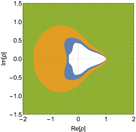
where , , and and are the number of links and relations in , respectively. In these models, an extension to a measure on exists if and only if (i.e. when the amplitude reduces to a real probability) Dowker et al. 2010; Surya and Zalel 2020. But, with our new understanding of as the algebra of covariant events in this model, we can ask whether there exists an extension to the strictly smaller when . (Note that this question is equivalent to asking whether there are measures on that do not extend to a measure on . When the measures are real probability measures, the answer is no: every measure on extens to a measure on . However, here we are concerned with complex measures, and it is unknown to the authors whether an analogous theorem holds in this case.) To this effect, we can apply equations (23-25) and the above criteria for extension by replacing with and the with the nodes of reduced poscau. This generalisation is possible since the results of Surya and Zalel 2020 rely only on the fact that labeled poscau is a finite-valency tree with no maximal elements, see Zalel 2021b for further discussion. The transition amplitudes on reduced poscau are fixed by requiring that (26) holds for principal causets and by imposing (23). We solved numerically for as a function of for . Our results (Fig.6) suggest that for any , there is a level above which the function takes its minimum on the nodes that contain principal causets, i.e. for all . If this is borne out then when and no extension to exists, meaning that Complex Transitive Percolation does not give rise to a well-defined quantum dynamics in this framework. Whether other classical cyclic dynamics can give rise to quantum dynamics via this formalism is an open question.
IV Observables from principal stem-sets
In section III we identified as a complete set of observables in cyclic dynamics, but it is unclear what is the physical meaning of each observable in this set. In this section, we identify a second algebra that forms a complete set of observables in cyclic dynamics and in which each observable has a clear physical interpretation.
We begin with terminology. We say that an order is a principal order if its representative is a principal causet. We say that is a principal stem-set if is a principal order. We define to be the set of principal stem-sets and write to denote the -algebra that they generate. We can now state our theorem:
Theorem 9.
Given , there exists some such that .
In perfect analogy to the result of Brightwell et al. 2003, the upshot of lemma 9 is that exhausts the set of observables in any cyclic dynamics, since the measure of any is fixed by the measure of some via .
Importantly, each event in is equivalent to a logical combination of statements about which principal orders are contained as stems in the growing causet, giving the observables in cyclic dynamics a clear physical interpretation. We will make the notion of “an order contained as a stem” precise after lemma 11.
We now prove theorem 9 through a series of lemmas.
Lemma 10.
Let denote a set of points and let denote an equivalence relation on . Let denote a standard Borel space. Let denote the Borel space derived from via the “covariance” property:
| (27) |
Let denote a countable family of sets that separates up to equivalence under , i.e. for any there exists a set in that contains but not . Then generates .
Proof.
Let denote the set of equivalence classes of elements of under and let denote the projection that maps each onto its equivalence class. Given , the quotient Borel space induced by is denoted by , where is the set of all such that .
The quotient Borel space is analytic whenever it is countably separated (second theorem on p.74 in Mackey 1976). In an analytic Borel space, any countable separating family is a generating family (corollary on p.73 in Mackey 1976). Therefore, any countable separating family in is a generating family.
Since is derived from via the “covariance” property, induces a bijection between and . Under this bijection, is mapped onto a countable separating family in . Since generates , and since bijections preserve countable set operations, generates . ∎
Lemma 11.
For any there exists a principal order such that and .
We will need the following terminology. Given a finite order and a (finite or infinite) causet , we say that is a stem in if there exists a stem in that is order-isomorphic to a representative of . If is a stem in and is a representative of , then we say that is a stem in . The cardinality of an order is defined to be equal to the cardinality of a representative of it. We use the term -stem to mean a stem of cardinality . We say than an order contains a break if its representative contains a break. The covering causet of is the principal causet formed from by placing an element above all . The covering order of is the order whose representative is a covering causet of some representative of .
Proof.
Let . Let denote the unlabeled past of the break in , so is an order that is a stem in . Note that may or may not be principal. Define similarly for . Note that and each contain breaks and therefore either or .
Let . Then there exists an such that for all .
Without loss of generality, let . We will show that . Suppose for contradiction that is a stem in . Then is the only -stem in is the only -stem in (since is the only -stem in , and “not a stem in any stem is not a stem”) is an unlabeled past of a break in there exists some such that , which is a contradiction. ∎
Corollary 12.
The countable family of sets,
| (28) |
separates up to equivalence under order-isomorphisms, i.e. for any there exists a set in that contains but not .
Lemma 13.
.
Proof.
We will show that both the LHS and the RHS are generated by the family , and the result follows.
We begin with the RHS. Note that is a Polish space (lemma 6 in Brightwell et al. 2003), and therefore its subspace is a standard Borel space (definition 1 on p.71 in Mackey 1976). The Borel space derived from via the “covariance” property (27) with respect to equivalence under order-isomorphism is equal to and contains the countable family of sets . Together, corollary 12 and lemma 10 imply that the family generates .
For the LHS, note that if a Borel space is generated by a family then its Borel subspace is generated by the family . ∎
Proof of theorem 9.
Consider some . Then such that , i.e. . ∎
V Posts
In the special case when the epochs are separated by posts, the dynamics satisfy , where is the event that the causet spacetime contains infinitely many posts, and the -algebra,
| (29) |
exhausts the covariant events, by analogy to the discussion of (4) and (14). The strictly stronger analogue of theorem 2 is,
Theorem 14.
.
Here, denotes the -algebra generated by the cylinder sets associated with those principal causets whose restriction is itself a principal causet. We call such a causet , and the cylinder set, order and stem-set associated with it, doubly principal. The analogue of theorem 9 is,
Theorem 15.
Given , there exists some in the -algebra generated by the doubly principal stem-sets such that .
Let us define a principal break to be a break whose past is a principal stem. Then there is a post if and only if there is a principal break: the post is the maximal element of the past of the principal break. The proof of theorems 14 and 15 can be obtained from the proofs of theorems 2 and 9 respectively, mutatis mutandis i.e. by replacing “break” with “principal break” and “principal stem” with “doubly principal stem”. So, for example, a segment is now defined to be the portion of the causet between two principal breaks and is always a principal causet.
Measures on correspond to walks up doubly-reduced poscau whose description is obtained from the description of reduced poscau (see section III.3) by replacing “principal” with “doubly principal” (so only doubly principal causets are contained in nodes of their own). Thus, cyclic models in which the epochs are separated by posts can be conceived of as random walks on this novel tree. Complex Transitive Percolation is such a cyclic model, and so we can extend the discussion in section III.4 by asking whether there exists an extension of the measure to the strictly smaller -algebra . We do so by modifying equations (23-25) and the criteria for extension by replacing with and the with the nodes of doubly-reduced poscau, but their application to Complex Transitive Percolation is inconclusive. On the one hand, we cannot prove that an extension exists since is equal to on every doubly principal causet so for all when . On the other hand, we can cannot rule out an extension, since every level in doubly-reduced poscau contains nodes with valency equal to 1 and on these nodes vanishes and therefore .
We now amend the extension criteria to provide further scrutiny in the special case where there are nodes with valency equal to 1. Let denote a finite-valency directed tree that contains no maximal elements and let denote the set of nodes at level . Let denote a node at level .
Define, , and note that an extension exists if and only if Surya and Zalel 2020.
Let be the set of level nodes that have valency greater than 1, and define,
| (30) | ||||
Then one can use definitions (30) to generalise the proof of claim 3.2 in Surya and Zalel 2020 and thus show that,
| (31) | ||||
Thus, if the right hand side of (31) diverges with then no extension exists.
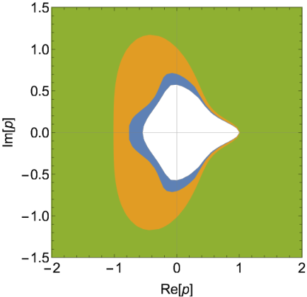
Applying this improved criterion to Complex Transitive Percolation on doubly-reduced poscau, our numerical solutions for as a function of for (Fig.7) suggest that for any , there exists a level above which the function restricted to the valency nodes takes its minimum value on the doubly principal causets, i.e. for all . If this is borne out then, when , the first term on the right hand side of (31) diverges as . Whether depends on the behaviour of in the second term. We note that, since is the sum over absolute values of amplitudes of reaching a doubly principal causet by stage , in future it could be computed using techniques similar to those used to obtain the probability of a post Bombelli et al. 2008.
VI Conclusion
In this work, we considered how the set of covariant observables can be distilled to a smaller exhaustive set of observables under the family of cyclic dynamics. This interplay between the kinematic constraint of covariance and the dynamic restriction to on-shell configurations (cyclic causets) gives rise to interrelated systems of sets with rich mathematical structure. In particular, we identified both and as exhaustive observable -algebras, and it is natural to ask how the two are related. First, note that both are sub-algebras of , since neither separates the set of rogues. Additionally, definition (14) of and theorem 9 combine to imply that: for any , there exists some such that , and vice versa, for any , there exists some such that . Therefore, under cyclic dynamics the two algebras of observables are equal up to sets of measure zero and can be considered equivalent. However, at the level of the kinematics the two -algebras are very different since the only events that they share are the unit and the empty set, as we now prove.
Lemma 16.
Let . If is contained in both and then is either the empty set or the unit element .
Proof.
Consider some causet and let denote the unlabeled past of the break in , so is an order which is a stem in . Define to be the causet which is some labeling of the disjoint union of the ’s. The event is the smallest event in that contains , in the sense that if then . The event is also the smallest event in that contains . Therefore any contains either both or neither of and .
Suppose . By definition of , either or . We show that in both cases, , which completes the proof.
Case(i): and . Note that contains some . Therefore, if then contains . Contradiction.
Case(ii): and . Note that there exists some causet that is not contained in and thefore . Contradiction. ∎
In particular, lemma 16 implies that . Therefore one cannot tell from the measure on whether the dynamics is cyclic, however if one knows the dynamics is cyclic then is an exhaustive set of observables. On the other hand, since , knowing the measure on is sufficient to determine whether the dynamics is cyclic.
Finally, our motivation for studying cyclic dynamics has been the key role that they play in the the causal set comological paradigm that aims to explain the emergence of a flat, homogeneous and isotropic cosmos directly from the quantum gravity era Sorkin 2000; Martin et al. 2001; Dowker and Zalel 2017. But what form do these models take and do they occupy a significant volume in theory space? The Transitive Percolation family of cyclic CSG model Alon et al. 1994; Rideout and Sorkin 2000 has served as a starting point for searches of cyclic models and some progress has been made in this direction: a class of cyclic dynamics in which epochs are separated by posts has been identified in Ash and McDonald 2005 and a conjecture of another class of such models has been put forward in Brightwell and Luczak 2016. But these formal results are yet to be fully understood and implemented (e.g., via computer simulations) and the characterisation of cyclic dynamics remains an important open question.
Acknowledgements: This research was supported in part by STFC grant ST/T000791/1. It was also supported in part by Perimeter Institute for Theoretical Physics. Research at Perimeter Institute is supported by the Government of Canada through Industry Canada and by the Province of Ontario through the Ministry of Economic Development and Innovation.
References
- Rideout and Sorkin (2000) D. P. Rideout and R. D. Sorkin, A Classical sequential growth dynamics for causal sets, Phys. Rev. D61, 024002 (2000), arXiv:gr-qc/9904062 [gr-qc] .
- Dowker (2020) F. Dowker, Being and Becoming on the Road to Quantum Gravity; or, the Birth of a Baby Is Not a Baby, in Beyond Spacetime, edited by N. Huggett, K. Matsubara, and C. Wüthrich (2020).
- Brightwell et al. (2003) G. Brightwell, H. F. Dowker, R. S. Garcia, J. Henson, and R. D. Sorkin, ‘Observables’ in causal set cosmology, Phys. Rev. D67, 084031 (2003), arXiv:gr-qc/0210061 [gr-qc] .
- Dowker and Surya (2006) F. Dowker and S. Surya, Observables in extended percolation models of causal set cosmology, Class. Quant. Grav. 23, 1381 (2006), arXiv:gr-qc/0504069 .
- Dowker (2014) F. Dowker, The birth of spacetime atoms as the passage of time, in Do We Need a Physics of ‘Passage’? Cape Town, South Africa, December 10-14, 2012 (2014) arXiv:1405.3492 [gr-qc] .
- Ahmed and Rideout (2010) M. Ahmed and D. Rideout, Indications of de Sitter Spacetime from Classical Sequential Growth Dynamics of Causal Sets, Phys. Rev. D 81, 083528 (2010), arXiv:0909.4771 [gr-qc] .
- Sorkin (2000) R. D. Sorkin, Indications of causal set cosmology, 3rd Peyresq Workshop on Quantum and Stochastic Gravity, String Cosmology and Inflation Peyresq, France, June 28-July 3, 1998, Int. J. Theor. Phys. 39, 1731 (2000), arXiv:gr-qc/0003043 [gr-qc] .
- Martin et al. (2001) X. Martin, D. O’Connor, D. P. Rideout, and R. D. Sorkin, On the ’renormalization’ transformations induced by cycles of expansion and contraction in causal set cosmology, Phys. Rev. D63, 084026 (2001), arXiv:gr-qc/0009063 [gr-qc] .
- Dowker and Zalel (2017) F. Dowker and S. Zalel, Evolution of Universes in Causal Set Cosmology, Comptes Rendus Physique 18, 246 (2017), arXiv:1703.07556 [gr-qc] .
- Dowker et al. (2020) F. Dowker, N. Imambaccus, A. Owens, R. Sorkin, and S. Zalel, A manifestly covariant framework for causal set dynamics, Class. Quant. Grav. 37, 085003 (2020), arXiv:1910.07292 [gr-qc] .
- Zalel (2021a) S. Zalel, The structure of covtree: searching for manifestly covariant causal set dynamics, Class. Quant. Grav. 38, 015001 (2021a), arXiv:2008.02607 [gr-qc] .
- Bento et al. (2022) B. V. Bento, F. Dowker, and S. Zalel, If time had no beginning: growth dynamics for past-infinite causal sets, Class. Quant. Grav. 39, 045002 (2022), arXiv:2109.10749 [gr-qc] .
- X et al. (2017) N. X, F. Dowker, and S. Surya, Scalar Field Green Functions on Causal Sets, Class. Quant. Grav. 34, 124002 (2017), arXiv:1701.07212 [gr-qc] .
- Glaser (2021) L. Glaser, Phase transitions in 2d orders coupled to the Ising model, Class. Quant. Grav. 38, 145017 (2021), arXiv:2011.13875 [gr-qc] .
- Kolmogorov and Fomin (1975) A. N. Kolmogorov and S. V. Fomin, Introductory Real Analysis (Dover Publications, New York, 1975).
- Brightwell et al. (2002) G. Brightwell, H. F. Dowker, R. S. Garcia, J. Henson, and R. D. Sorkin, General covariance and the ’Problem of time’ in a discrete cosmology, in Alternative Natural Philosophy Association Meeting Cambridge, England, August 16-21, 2001 (2002) arXiv:gr-qc/0202097 [gr-qc] .
- Bombelli et al. (2008) L. Bombelli, I. Seggev, and S. Watson, A Computation of the Expected Number of Posts in a Finite Random Graph Order, (2008), arXiv:0809.2258 [math.CO] .
- Alon et al. (1994) N. Alon, B. Bollobás, G. Brightwell, and S. Janson, Linear extensions of a random partial order, Ann. Applied Prob. 4, 108 (1994).
- Ash and McDonald (2003) A. Ash and P. McDonald, Moment problems and the causal set approach to quantum gravity, J. Math. Phys. 44, 1666 (2003), arXiv:gr-qc/0209020 .
- Ash and McDonald (2005) A. Ash and P. McDonald, Random partial orders, posts, and the causal set approach to discrete quantum gravity, J. Math. Phys. 46, 062502 (2005).
- Brightwell and Luczak (2016) G. Brightwell and M. Luczak, The mathematics of causal sets, in Recent Trends in Combinatorics, The IMA Volumes in Mathematics and its Applications, Vol. 159 (Springer, Cham, 2016).
- Dowker et al. (2010) F. Dowker, S. Johnston, and S. Surya, On extending the Quantum Measure, J. Phys. A43, 505305 (2010), arXiv:1007.2725 [gr-qc] .
- Surya and Zalel (2020) S. Surya and S. Zalel, A Criterion for Covariance in Complex Sequential Growth Models, Class. Quant. Grav. 37, 195030 (2020), arXiv:2003.11311 [math-ph] .
- Zalel (2021b) S. Zalel, Discrete Random Spacetimes: Covariance and Quantization in Growth Dynamics for Causal Sets, Ph.D. thesis, Imperial Coll., London (2021b).
- Mackey (1976) G. Mackey, Theory of Unitary Group Representations (University of Chicago Press, 1976).