Fair Graphical Resource Allocation with
Matching-Induced Utilities

Zheng Chen Bo Li Mingming Li Guochuan Zhang Affiliation: College of Computer Science and Technology, Zhejiang University, Hangzhou, China{21721122, zgc}@zju.edu.cn Affiliation: College of Computer Science and Technology, Zhejiang University, Hangzhou, China{21721122, zgc}@zju.edu.cn Affiliation: Department of Computing, The Hong Kong Polytechnic University, Hong Kongcomp-bo.li@polyu.edu.hk Affiliation: Department of Computer Science, City University of Hong Kong, Hong Kongminming.li@cityu.edu.hk

April 2022

Abstract

Motivated by real-world applications, we study the fair allocation of graphical resources, where the resources are the vertices in a graph. Upon receiving a set of resources, an agent’s utility equals the weight of a maximum matching in the induced subgraph. We care about maximin share (MMS) fairness and envy-freeness up to one item (EF1). Regarding MMS fairness, the problem does not admit a finite approximation ratio for heterogeneous agents. For homogeneous agents, we design constant-approximation polynomial-time algorithms, and also note that significant amount of social welfare is sacrificed inevitably in order to ensure (approximate) MMS fairness. We then consider EF1 allocations whose existence is guaranteed. However, the social welfare guarantee of EF1 allocations cannot be better than $1/n$ for the general case, where $n$ is the number of agents. Fortunately, for three special cases, binary-weight, two-agents and homogeneous-agents, we are able to design polynomial-time algorithms that also ensure a constant fractions of the maximum social welfare.

1 Introduction

Resource allocation has been actively studied due to its practical applications (Moulin 2003; Goldman and Procaccia 2014; Flanigan et al. 2021). Traditionally, the utilities are assumed to be additive which means an agent’s value for a bundle of resources equals the sum of each single item’s marginal utility. But in many real-world problems, the resources have graph structures and thus the agents’ utilities are not additive but depend on the structural properties of the received resources. For example, Peer Instruction (PI) has been shown to be an effective learning approach based on a project conducted at Harvard University, and one of the simplest ways to implement PI is to pair the students (Crouch and Mazur 2001). Consider the situation when we partition students to advisors, where the advisors will adopt PI for their assigned students. Note that the advisors may hold different perspectives on how to pair the students based on their own experience and expertise, and they want to maximize the efficiency of conducting PI in their own assigned students. How should we assign the students fairly to the advisors? How can we maximize the social welfare among all (approximately) fair assignments? In this work, we take an algorithm design perspective to solve these two questions. Similar pairwise joint work also appears as long-trip coach driver vs. co-driver and accountant vs. cashier, which is widely investigated in matching theory (Lovász and Plummer 2009).

The graphical nature of resources has been considered in the literature (see, e.g., (Bouveret et al. 2017; Suksompong 2019; Bilò et al. 2019; Igarashi and Peters 2019)). In this line of research, the graph is used to characterize feasible allocations, such as the resources allocated to each agent should be connected, but the agents still have additive utilities over allocated items. We refer the readers to (Suksompong 2021) for a comprehensive survey of constrained fair division. As shown by the previous PI an other examples, with graphical resources, the value of a set of resources does not solely depend on the vertices or the edge weights, but decided by the combinatorial structure of the subgraph, such as the maximum matching in our problem.

Our problem also aligns the research of balanced graph partition (Miyazawa et al. 2021). Although there are heuristic algorithms in the literature (Kress et al. 2015; Barketau et al. 2015) that partition a graph when the subgraphs are evaluated by maximum matchings, these algorithms do not have theoretical guarantees. Our first fairness criterion is the maximin share (MMS) fairness proposed by Budish 2011, which generalizes the max-min objective in Santa Claus problem (Bansal and Sviridenko 2006). Informally, the MMS value of an agent is her best guarantee if she is to partition the graph into several subgraphs but receives the worst one. We aim at designing efficient algorithms with provable approximation guarantees. As will be clear later, to achieve (approximate) MMS fairness, a significant amount of social welfare has to be inevitably sacrificed. Our second fairness notion is envy-freeness (EF) (Foley 1967). In an EF allocation, no agent prefers the allocation of another agent to her own. Since the resources are indivisible, such an allocation barely exists, and recent research in fair division focuses on achieving its relaxations instead. One of the most widely accepted and studied relaxations is envy-freeness up to one item (EF1) (Budish 2011), which requires the envy to be eliminated after removing one item. Lipton et al. 2004 proved that an EF1 allocation always exists even with combinatorial valuations.¹¹ 1 The algorithm in (Lipton et al. 2004) was originally published in 2004 with a different targeting property. In 2011, Budish 2011 formally proposed the notion of EF1 fairness. It is noted that an arbitrary EF1 allocation may have low social welfare, and our goal is to compute an EF1 allocation which preserves a large fraction of the maximum social welfare without fairness constraints. The social welfare loss by enforcing the allocations to be EF1 is quantified by price of EF1 (Bei et al. 2021).

1.1 A Summary of Results

We study the fair allocation of graphical resources when the resources are indivisible and correspond to the vertices in the graph, and the agents’ valuations are measured by the weight of the maximum matchings in the induced subgraphs. The fairness of an allocation is measured by maximin share (MMS) and envy-free up to one item (EF1). Our model strictly generalizes the additive setting: it degenerates to the additive setting when the graph consists of a set of independent edges by regarding each edge as an item whose value is the weight of the edge. This is because the removal of a vertex also removes the adjacent edge. We aim at designing efficient algorithms that compute fair allocations with high social welfare. Our main results are summarized as follows.

We first consider MMS fairness and find that no algorithm has bounded approximation ratio even if there are two agents with binary weights. We thus focus on the homogeneous case when the agents have identical valuations. Then our problem degenerates to the max-min objective, i.e., partitioning the vertices so that the minimum weight of the maximum matchings in the subgraphs is maximized. It is easy to see that an MMS fair allocation always exists but finding it is NP-hard. Accordingly, we design a polynomial-time $1/8$ -approximation algorithm for arbitrary number of agents, and show that when the problem only involves two agents, the approximation ratio can be improved to $2/3$ . It is noted that, to ensure any finite approximation of MMS fairness, significant amount of social welfare is inevitably sacrificed.

We then study EF1 allocation whose existence is guaranteed Lipton et al. 2004. We prove that there exist instances for which none of the EF1 allocations can ensure better than $1/n$ fraction of the maximum social welfare. But this result does not exclude the possibility of constant approximations for special cases. In particular, we consider three cases: (1) binary-weight functions, (2) two-agents, (3) homogeneous-agents. For each setting, we design polynomial-time algorithms that compute EF1 allocations whose social welfare is at least a constant fraction of the maximum social welfare that can be achieved without fairness constraints.

1.2 Related Works

Two separate research lines are closely related to our work, namely graph partition and fair division.

Graph Partition. Partitioning graphs into balanced subgraphs has been extensively studied in operations research (Miyazawa et al. 2021) and computer science (Buluç et al. 2016). There are several popular objectives for evaluating whether a partition is balanced. Among the most prominent ones are the max-min (or min-max) objectives, where the goal is to maximize (or minimize) the total weight of the minimum (or maximum) part. Particularly, the vehicle routing problem (VRP) (Koç et al. 2016), which generalizes the travelling salesperson problem (TSP), is closely related to our work. It asks for an optimal set of routes for a number of vehicles, to visit a set of customers. There are a number of popular variants for the VRP, e.g., the so called heterogeneous vehicle routing problem (Yaman 2006; Rathinam et al. 2020). There are many other combinatorial structures studied in graph partitioning problems. For example, in the min-max tree cover (a.k.a. nurse station location) problem, the task is to use trees to cover an edge-weighted graph such that the largest tree is minimized (Khani and Salavatipour 2014). This problem also falls under the umbrella of a more general problem, the graph covering problem, where a set of pairwise disjoint subgraphs (called templates) is used to cover a given graph, such as paths (Farbstein and Levin 2015), cycles (Traub and Tröbst 2020), and matchings (Kress et al. 2015).

Fair Division. Allocating a set of indivisible items among multiple agents is a fundamental problem in the fields of multi-agent systems and computational social choice, and we refer the readers to recent surveys (Amanatidis et al. 2022; Aziz et al. 2022) for more detailed discussion. Envy-freeness (EF) and maximin share fairness (MMS) are two well accepted and extensively studied solution concepts. However, with indivisible items, these requirements are demanding and thus the state-of-the-art research mostly studies their relaxations and approximations. For example, EF1 allocation is studied as a relaxation of EF which always exists (Lipton et al. 2004). Various constant approximation algorithms for MMS allocations are proposed in (Kurokawa et al. 2018; Garg and Taki 2021) for additive valuations and in (Barman and Krishnamurthy 2020; Ghodsi et al. 2018) for subadditive valuations. Our work focuses on indivisible graphical items where agents have combinatorial valuations (neither subadditive nor superadditive) depending on the structural properties. Moreover, all the existing algorithms for non-additive valuations run in polynomial time only if the computation of valuations is assumed to be effortless (i.e., oracles). In contrast, in this work, we aim at designing truly polynomial-time approximation algorithms without valuation oracles.

2 Preliminaries

Denote by $G=(V,E)$ an undirected graph with no reflexive edges, where $V$ contains all vertices and $E$ contains all edges. The vertices are the resources, also called items, that are to be allocated to $n$ heterogeneous agents, denoted by $N$ . Each agent $i$ has an edge weight function $w_{i}:E\to{\mathbb{R}}^{+}\cup\{0\}$ , which may be different from others’. If $w_{i}(e)\in\{0,1\}$ for all $e\in E$ , then the weight function is called binary. Let $\mathbf{w}=(w_{1},\cdots,w_{n})$ . A matching $M\subseteq E$ is a set of vertex-disjoint edges, and let $w_{i}(M)=\sum_{e\in M}w_{i}(e)$ . Let $M(V)$ be the maximum (weighted) matching within the induced subgraph $G[V]$ . For any subgraph $G^{\prime}$ , let $V(G^{\prime})$ and $E(G^{\prime})$ be the sets of vertices and edges in $G^{\prime}$ , respectively. An allocation $\mathbf{X}=(X_{1},\cdots,X_{n})$ is a partition of $V$ such that $\cup_{i\in N}X_{i}=V$ and $X_{i}\cap X_{j}=\emptyset$ for $i\neq j$ . If $\bigcup_{i\in N}X_{i}\subsetneq V$ , the allocation is called partial. Each agent $i$ has a utility function $u_{i}:2^{V}\to{\mathbb{R}}^{+}\cup\{0\}$ , where $u_{i}(X_{i})$ equals the weight of a maximum (weighted) matching in $G[X_{i}]$ . When the agents have identical valuations (i.e., homogeneous agents), we omit the subscript and use $w(\cdot)$ and $u(\cdot)$ to denote all agents’ weight and utility functions. A problem instance is denoted by $\mathcal{I}=(G,N)$ . When we want to highlight the weight function, $w$ is also included as a parameter, i.e., $\mathcal{I}=(G,N,w)$ .

Next, we introduce the solution concepts. Our first fairness notion is maximin share (MMS) (Budish 2011). Letting $\Pi_{n}(V)$ be the set of all $n$ -partitions of $V$ , the maximin share of agent $i$ is

\mathsf{MMS}_{i}(\mathcal{I})=\max_{\mathbf{X}\in\Pi_{n}(V)}\min_{j\in N}u_{i}(X_{j}).

We may write $\mathsf{MMS}_{i}$ for short if $\mathcal{I}$ is clear from the context. Therefore agent $i$ is satisfied regarding MMS fairness if her utility is no smaller than $\mathsf{MMS}_{i}$ .

Definition 2.1 ( $\alpha$ -MMS).

For any $\alpha\geq 0$ , an allocation $\mathbf{X}=(X_{1},\cdots,X_{n})$ is called $\alpha$ -approximate maximin share ( $\alpha$ -MMS) fair if for all agents $i\in N$ ,

u_{i}(X_{i})\geq\alpha\cdot\mathsf{MMS}_{i}.

The allocation is called MMS fair if $\alpha=1$ .

The second fairness notion is about envy-freeness (EF). An allocation $\mathbf{X}$ is called EF if no agent envies any other agent’s bundle, i.e.,

u_{i}(X_{i})\geq u_{i}(X_{j})\text{ for all agents $i,j\in N$.}

EF is very hard to satisfy; consider a simple example, where the graph is a triangle and two agents have weight 1 for all edges. Then in every allocation, there is one agent who gets at most one vertex (with utility 0) and the other agent gets at least two vertices (which contains an edge and thus has utility 1). Accordingly, we focus on envy-free up to one item instead (Budish 2011).

Definition 2.2 (EF1).

An allocation $\mathbf{X}=(X_{1},\cdots,X_{n})$ is called envy-free up to 1 item (EF1) if for any $i$ and $j$ , there exists $g\in X_{j}$ such that $u_{i}(X_{i})\geq u_{i}(X_{j}\setminus\{g\})$ .

Besides fairness, we also want the allocation to be efficient. Given an allocation $\mathbf{X}=(X_{1},\cdots,X_{n})$ , the social welfare of $\mathbf{X}$ is $\mathsf{sw}(\mathbf{X})=\sum_{i\in N}u_{i}(X_{i})$ . Note that given any instance $\mathcal{I}$ , the best possible social welfare of any allocation is the weight of a maximum matching in the graph $G$ by setting the weight of each edge to $\max_{i\in N}w_{i}(e)$ , which is denoted by $\mathsf{sw}^{*}(\mathcal{I})$ . If the instance $\mathcal{I}$ is clear from the context, we also denote $\mathsf{sw}^{*}(\mathcal{I})$ as $\mathsf{sw}^{*}$ for short.

3 MMS Fair Allocations

3.1 Heterogeneous Agents

Theorem 3.1.

No algorithm has bounded approximation guarantee for MMS, even if there are two agents with non-identical binary weight functions on the graph.

Proof.

Consider the example as shown in Figure 1. The graph containing four nodes $\{v_{1},v_{2},v_{3},v_{4}\}$ is allocated to two agents whose valuations (i.e., edge weights) are shown in Figure 1(a) and 1(b) respectively. It can be verified that $\mathsf{MMS}_{i}=1$ for both $i=1,2$ . However, no matter how we allocate the vertices to the agents, one of them receives utility of $0$ .

Refer to caption — (a) Agent $1$ ’s Metric

∎

Theorem 3.1 is very strong in the sense that it excludes the possibility of designing algorithms with bounded approximation ratio for MMS even for the special cases of two-agent or binary weight functions.

3.2 Homogeneous Agents

Due to the strong impossibility, we study the case of identical valuations, where MMS fairness degenerates to the max-min objective, where the problem is to partition a graph into $n$ subgraphs so that the smallest weight of the maximum matchings in these subgraphs is maximized. It is easy to see that finding such an allocation is NP-hard even when there are two agents and the graph only consists of independent edges, which is essentially a Partition problem. Thus, our target is polynomial-time approximation algorithms. Without loss of generality, in this section, we assume $w(e)\geq 1$ for all $e\in E$ . Since the agents are identical, the subscript in $\mathsf{MMS}_{i}$ is omitted. Our main result in this section is as follows.

Theorem 3.2.

For homogeneous agents, we can compute a $1/8$ -MMS allocation in polynomial time.

Given an instance $\mathcal{I}=(G,N)$ , to design such an algorithm with guaranteed approximation of MMS fairness, the thought at a glance is to allocate a maximum matching in $G$ . That is, we compute a maximum matching $M^{*}\subseteq E$ , and then partition $M^{*}$ into $n$ bundles $(M_{1},\cdots,M_{n})$ where $w(M_{1})\geq\cdots\geq w(M_{n})$ such that $w(M_{n})$ is as large as possible. However, such an allocation can be arbitrarily bad, let alone maximizing the minimum bundle being an NP-hard problem. Consider an example with two agents and the graph is shown in Figure 2 where $\Delta>1$ is arbitrarily large. Any allocation with bounded approximation ratio of MMS fairness ensures that every agent has value 1, but by partitioning the maximum matching (which contains a single edge with weight $\Delta$ ) the smaller bundle has value 0.

Before describing our algorithm, we first define greedy partition of the maximum matching.

Greedy Partition.

Given a matching $M$ , partition $M$ into $\Gamma(M)=(M_{1},\cdots,M_{n})$ as follows.

•

Sort and rename the edges in $M$ such that $w(e_{1})\geq\cdots\geq w(e_{k})$ where $k=|M|$ .
•

Initially set $M_{1}=\cdots=M_{n}=\emptyset$ .
•

For $i=1,\cdots,k$ , select $j$ such that $w(M_{j})\leq w(M_{j^{\prime}})$ for all $j^{\prime}$ and set $M_{j}=M_{j}\cup\{e_{i}\}$ .
•

Sort and rename $M_{1},\cdots,M_{n}$ so that $w(M_{1})\geq\cdots\geq w(M_{n})$ .

The greedy partition $(M_{1},\cdots,M_{n})$ of the maximum matching $M^{*}$ corresponds to an allocation of vertices where unmatched vertices $V^{\prime}=V\setminus\cup_{i\in N}V(M_{i})$ can be allocated arbitrarily. Although this allocation might not be good in general, when the graph is unweighted ( $w(e)=w(e^{\prime})$ for all $e,e^{\prime}\in E$ ) or $|M_{1}|\geq 2$ , it ensures a good approximation.

Lemma 3.3.

If $G$ is unweighted, the greedy partition $(M_{1},\cdots,M_{n})$ of $M^{*}$ is an MMS allocation.

Proof.

Without loss of generality, assume all edges have weight 1. In the greedy partition $(M_{1},\cdots,M_{n})$ of $M^{*}$ , for any $i\in N$ ,

|M_{i}|\geq|M_{n}|=\lfloor\frac{|M^{*}|}{n}\rfloor.

Let $(O_{1},\cdots,O_{n})$ be an optimal max-min allocation. If $\mathsf{MMS}=|M(O_{n})|>|M_{n}|$ , then for all $i\in N$ ,

|M(O_{i})|\geq\lfloor\frac{|M^{*}|}{n}\rfloor+1.

Thus

\displaystyle\sum_{i\in N}|M(O_{i})|\geq n\cdot\lfloor\frac{|M^{*}|}{n}\rfloor+n>|M^{*}|,

which is a contradiction with $M^{*}$ being a maximum matching. ∎

Lemma 3.4.

If $|M_{1}|\geq 2$ , $\Gamma(M^{*})$ corresponds to an allocation that is $1/2$ -MMS fair.

Proof.

Denote by $O=(O_{1},O_{2},\cdots,O_{n})$ the optimal solution, where $u(O_{1})\geq u(O_{2})\geq\cdots\geq u(O_{n})$ and $\mathsf{MMS}(\mathcal{I})=u(O_{n})$ . Under the maximum matching $M$ , consider the greedy partition $(M_{1},M_{2},\cdots,M_{n})$ , where $u(M_{1})\geq u(M_{2})\geq\cdots\geq u(M_{n})$ . In greedy partition procedure, all edges are sorted in descending order of their weights and each time we select the edge with the largest weight in the remaining edge set and allocate it to the bundle with the least total utility. If $|M_{1}|\geq 2$ , consider the last edge $e$ added to $M_{1}$ , we have $w(M_{n})\geq w(e)$ , since there exists at least one edge added to $M_{n}$ before edge $e$ is added to $M_{1}$ . Since in the greedy procedure, edges are added to the bundle with least utility, we have $w(M_{n})\geq w(M_{1}\setminus\{e\})$ . Furthermore, we have

	$\displaystyle w(M_{n})$	$\displaystyle\geq\frac{1}{2}(w(e)+w(M_{1}/{e}))\geq\frac{1}{2}w(M_{1})$
		$\displaystyle\geq\frac{1}{2n}\sum\limits_{i=1}^{n}w(M_{i})\geq\frac{1}{2n}\sum\limits_{i=1}^{n}u(O_{i})$
		$\displaystyle\geq\frac{1}{2}u(O_{n}),$

and the lemma holds accordingly. ∎

The tricky case is when $M_{1}$ contains a single edge $e^{*}$ . The greedy partition fails because $w(e^{*})$ is too large so that very few edges or edges with very small weights can be put in $M_{i}$ ’s for $i\geq 2$ . One way to overcome this difficulty is to decrease the weight of $e^{*}$ and re-compute a maximum matching, through which the advantage of $e^{*}$ can diminish. For simplicity, assume all edge weights are powers of 2. This is without much loss of generality which decreases the approximation ratio by at most $1/2$ .

Lemma 3.5.

Let $\mathcal{I}^{\prime}=(G,N,w^{\prime})$ be the instance obtained from $\mathcal{I}=(G,N,w)$ by rounding all edge weights down to nearest powers of 2. If $(X_{1},\cdots,X_{n})$ is an $\alpha$ -MMS allocation of $\mathcal{I}^{\prime}$ , it is also an $\alpha/2$ -MMS allocation of $\mathcal{I}$ .

Proof.

Let $\mathcal{I}^{\prime\prime}=(G,N,w^{\prime\prime})$ be the instance obtained from $\mathcal{I}$ by halving all its edge weights. It is easy to see that

\mathsf{MMS}(\mathcal{I}^{\prime\prime})=\frac{1}{2}\cdot\mathsf{MMS}(\mathcal{I}).

Moreover, the weight of all edges in instance $\mathcal{I}^{\prime}$ is at least as large as that in instance $\mathcal{I}^{\prime\prime}$ , and thus

\mathsf{MMS}(\mathcal{I}^{\prime})\geq\mathsf{MMS}(\mathcal{I}^{\prime\prime})=\frac{1}{2}\cdot\mathsf{MMS}(\mathcal{I}).

Finally, since $u_{i}(X_{i})\geq\alpha\cdot\mathsf{MMS}(\mathcal{I}^{\prime})$ for all $i\in N$ , then

u_{i}(X_{i})\geq\frac{\alpha}{2}\cdot\mathsf{MMS}(\mathcal{I}),

and thus the lemma holds. ∎

Now we are ready to describe our Algorithm 1. We first compute a maximum matching $M^{*}$ and its greedy partition $\Gamma(M^{*})=(M_{1},\cdots,M_{n})$ such that $w(M_{1})\geq\cdots\geq w(M_{n})$ . If $|M_{1}|\geq 2$ , by Lemmas 3.4 and 3.5, we can directly output the corresponding partition of vertices so that the approximation ratio is at least $1/4$ . If $|M_{1}|=1$ , we consider two cases. When $w(M_{n})\geq 1/2\cdot w(M_{1})$ , $w(M_{n})$ is still not too small and we can stop the algorithm with a constant approximation ratio. However, if $w(M_{n})<1/2\cdot w(M_{1})$ , it means the utility of the smallest bundle is much less than that of the largest bundle. Then we update the edge weights: Let $H$ be the edges with weights no smaller than $w(e_{1})$ where $e_{1}$ is the edge in $M_{1}$ , and decrease all their weights to $1/2\cdot w(e_{1})$ . By repeating this procedure, eventually we reach an allocation for which $w(M_{n})\geq 1/2\cdot w(M_{1})$ or $|M_{1}|\geq 2$ .

0: Instance

\mathcal{I}=(G,N)

with

G=(V,E;w)

0: Allocation

\mathbf{X}=(X_{1},\cdots,X_{n})

1: For all

e\in E

, reset

w(e)=2^{\lfloor\log w(e)\rfloor}.

2: Find a maximum matching

M^{*}

G

. Denote by

V^{\prime}

the set of unmatched vertices.

3: Find the greedy partition

\Gamma(M^{*})=(M_{1},\cdots,M_{n})

M^{*}

such that

w(M_{1})\geq\cdots\geq w(M_{n})

4: while

w(M_{1})>2\cdot w(M_{n})

and

G

has different weights do

5: Let

e_{1}

be the edge in

M_{1}

and

H=\{e\in E\mid w(e)\geq w(e_{1})\}

6: Let

w(e)=w(e_{1})/2

for all

e\in H

7: Re-compute a maximum matching

M^{*}

8: Re-set

V^{\prime}

to be unmatched vertices by

M^{*}

9: Re-compute the greedy partition

\Gamma(M^{*})=(M_{1},\cdots,M_{n})

such that

w(M_{1})\geq\cdots\geq w(M_{n})

10: end while

11: Set

X_{i}=V(M_{i})

for

i=1,\cdots,n-1

12: Set

X_{n}=V(M_{n})\cup V^{\prime}

13: Return allocation

(X_{1},\cdots,X_{n})

Algorithm 1 Approximately MMS Fair Algorithm

Proof of Theorem 3.2.

First, we show Algorithm 1 is well-defined and runs in polynomial time. Every time when the condition of the while loop holds, either the graph has different weights and an allocation is returned or the weights of the heaviest edges are decreased by $1/2^{k}$ with some $k\geq 1$ . Thus the while loop is executed $O(\max_{e\in E}\log w(e))$ rounds.

Next we prove the approximation ratio. By Lemma 3.5, we only need to consider the instance where the edge weights are powers of 2 and show the allocation is 1/4-approximate MMS fair. Denote by $O=(O_{1},\cdots,O_{n})$ the optimal solution, where $u(O_{1})\geq\cdots\geq u(O_{n})$ and $\mathsf{MMS}(\mathcal{I})=u(O_{n})$ . The first time when we reach the while loop, if $w(M_{1})\leq 2\cdot w(M_{n})$ ,

w(M_{n})\geq\frac{1}{2}\cdot w(M_{1})\geq\frac{1}{2}\cdot u(O_{n})=\frac{1}{2}\cdot\mathsf{MMS}(\mathcal{I}),

where the second inequality holds because $M^{*}$ is a maximum matching in $G$ . Thus the allocation is 1/2-MMS. If all edges have the same weight, then by Lemma 3.3, the allocation is optimal.

We move into the while loop if $w(M_{1})>2\cdot w(M_{n})$ and the edge weights are not identical. Note that $w(M_{1})>2\cdot w(M_{n})$ implies $M_{1}$ contains a single edge denoted by $e_{1}$ . Otherwise consider the last edge added to $M_{1}$ in the greedy partition, denoted by $e^{\prime}$ . Then $w(M_{1}\setminus\{e^{\prime}\})\leq w(M_{n})$ and $w(e^{\prime})\leq w(M_{n})$ , which implies $w(M_{1})\leq 2\cdot w(M_{n})$ . After the while loop, denote by $\mathcal{I}^{\prime}$ the instance, by $w^{\prime}(\cdot)$ the new weights with new utility function $u^{\prime}(\cdot)$ , by $O^{\prime}=(O^{\prime}_{1},\cdots,O^{\prime}_{n})$ the new optimal solution and by $M^{\prime}$ the maximum matching with greedy partition $(M^{\prime}_{1},\cdots,M^{\prime}_{n})$ . Then we have the following claim.

Claim 3.6.

After each while loop, one of the following two cases holds.

•

Case 1. $w(e_{1})\geq 2\cdot\mathsf{MMS}(\mathcal{I})$ , then $\mathsf{MMS}(\mathcal{I}^{\prime})=\mathsf{MMS}(\mathcal{I})$ ;
•

Case 2. $w(e_{1})<2\cdot\mathsf{MMS}(\mathcal{I})$ , then $2\cdot\mathsf{MMS}(\mathcal{I}^{\prime})>\mathsf{MMS}(\mathcal{I})$ and $w^{\prime}(M^{\prime}_{1})\leq 2\cdot w^{\prime}(M^{\prime}_{n})$ .

Proof.

We first consider Case 1. For any $O_{i}$ , if $w(e)<w(e_{1})$ for all $e\in M(O_{i})$ , then $u(O_{i})$ does not decrease. If $w(e)\geq w(e_{1})$ for some $e\in M(O_{i})$ , $u(O_{i})\geq w(e_{1})\geq 2\cdot\mathsf{MMS}(\mathcal{I})$ and after decreasing the weights to $w(e_{1})/2$ , $u^{\prime}(O_{i})\geq\mathsf{MMS}(\mathcal{I})$ , implying the existence of an allocation with the minimum utility no smaller than $\mathsf{MMS}(\mathcal{I})$ , which means $\mathsf{MMS}(\mathcal{I}^{\prime})=\mathsf{MMS}(\mathcal{I})$ .

Second, we consider Case 2 when $w(e_{1})<2\cdot\mathsf{MMS}(\mathcal{I})$ . It is straightforward that $2\cdot\mathsf{MMS}(\mathcal{I}^{\prime})>\mathsf{MMS}(\mathcal{I})$ since $w(e_{1})>\mathsf{MMS}(\mathcal{I})$ (If $w(e_{1})=\mathsf{MMS}(\mathcal{I})$ , then $w(e_{1})=w(M_{1})=\cdots=w(M_{n})=\mathsf{MMS}(\mathcal{I})>\frac{1}{2}w(M_{n})$ , since $M^{*}$ is a maximum (weighted) matching. The Algorithm 1 moves out of the while loop and returns the optimal solution), and after decreasing the weights of some edges to $w(e_{1})/2$ , $u^{\prime}(O_{i})\geq w(e_{1})/2>\mathsf{MMS}(\mathcal{I})/2$ (If $e_{1}\in M(O_{i})$ , $u^{\prime}(O_{i})\geq w(e_{1})/2$ . Otherwise, $u^{\prime}(O_{i})=u(O_{i})\geq\mathsf{MMS}(\mathcal{I})>\mathsf{MMS}(\mathcal{I})/2$ ). Next we show $|M^{\prime}_{1}|\geq 2$ which implies $w^{\prime}(M^{\prime}_{1})\leq 2\cdot w^{\prime}(M^{\prime}_{n})$ . For the sake of contradiction, assume $M^{\prime}_{1}=\{e^{\prime}_{1}\}$ . Therefore, we derive $w^{\prime}(e^{\prime}_{1})=w^{\prime}(M^{\prime}_{1})\geq\cdots\geq w^{\prime}(M^{\prime}_{n})$ , and thus

w^{\prime}(M^{\prime})\leq n\cdot w^{\prime}(e^{\prime}_{1})<n\cdot w^{\prime}(O^{\prime}_{n})\leq\sum_{i\in N}w^{\prime}(O^{\prime}_{i}).

This is a contradiction with $M^{\prime}$ being a maximum matching in $G$ , which completes the proof. ∎

By Claim 3.6, the while loop will not execute Case 2 or it executes Case 1 for several times and then Case 2 for exactly once. If Case 2 is not executed, then the allocation is 1/2-MMS fair and the analysis is the same with the case when the while loop is not executed.

If Case 2 is executed once, then by Claim 3.6,

w^{\prime}(M^{\prime}_{n})\geq\frac{1}{2}\cdot w^{\prime}(M^{\prime}_{1})\geq\frac{1}{2}\cdot\mathsf{MMS}(\mathcal{I}^{\prime})\geq\frac{1}{4}\cdot\mathsf{MMS}(\mathcal{I}).

Finally, by Lemma 3.5, the allocation is 1/8-MMS for any instance with arbitrary weights. ∎

When $n=2$ , we can improve Algorithm 1 and obtain a better approximation ratio of 2/3. Algorithm 2 is similar with Algorithm 1; we first compute a maximum matching $M^{*}$ and a max-min partition $(M_{1},M_{2})$ with $w(M_{1})\geq w(M_{2})$ . If $w(M_{1})>2w(M_{2})$ , we output the corresponding allocation. Otherwise, in graph $G$ , we directly delete the edge that $M_{1}$ contains. We repeat the above procedure until all edges are removed.

0: Instance

\mathcal{I}=(G,N,u)

with

G=(V,E;w)

0: Allocation

\mathbf{X}=(X_{1},X_{2})

1: Find a maximum matching

M^{*}

G

. Denote by

V^{\prime}

the set of unmatched vertices by

M^{*}

2: Find the greedy partition

(M_{1},M_{2})

of edges in

M^{*}

such that

w(M_{1})\geq w(M_{2})

3: Let

Max=w(M_{2})

4: Set

X_{1}=V(M_{1})

5: Set

X_{2}=V(M_{2})\cup V^{\prime}

6: while

w(M_{1})>2w(M_{2})

7: // Note that if the while loop is entered, then

|M_{1}|=1

8: By Lemma 3.4.

M_{1}

must contain only one edge. Suppose

M_{1}=\{e^{*}\}

9: Delete edge

e^{*}

10: Re-compute a maximum matching

M^{*}

11: Re-set

V^{\prime}

to be unmatched vertices by

M^{*}

12: Re-compute the greedy partition

(M_{1},M_{2})

M^{*}

such that

w(M_{1})\geq w(M_{2})

13: if

Max<w(M_{2})

then

14:

Max=w(M_{2})

15: Set

X_{1}=V(M_{1})

16: Set

X_{2}=V(M_{2})\cup V^{\prime}

17: end if

18: end while

19: Output allocation

(X_{1},X_{2})

Algorithm 2 Max-Min Allocation for 2 Agents

Theorem 3.7.

Algorithm 2 outputs an allocation that is $2/3$ -approximate max-min fair in polynomial time .

Proof.

Given an Instance $\mathcal{I}=(G,N,u)$ with $G=(V,E;w)$ . Denote by $O=(O_{1},O_{2})$ the optimal solution, where $u(O_{1})\geq u(O_{2})$ and $\mathsf{MMS}(\mathcal{I})=u(O_{2})$ . The first time when we reach the while loop, if $w(M_{1})\leq 2\cdot w(M_{2})$ , allocation $(X_{1},X_{2})=(V(M_{1}),V(M_{2})\cup V^{\prime})$ has been output. By Algorithm 2, we have

w(M_{1})\geq u(O_{1})\geq u(O_{2})\geq w(M_{2}).

Moreover,

	$\displaystyle w(M_{2})$	$\displaystyle\geq\frac{1}{3}\cdot(w(M_{1})+w(M_{2}))$
		$\displaystyle\geq\frac{1}{3}\cdot(u(O_{1})+u(O_{2}))$
		$\displaystyle\geq\frac{1}{3}\cdot 2\cdot u(O_{2})=\frac{2}{3}\cdot u(O_{2}).$

We move into the while loop if $w(M_{1})>2\cdot w(M_{2})$ . In such case, $M_{1}$ contains only one edge, i.e., $|M_{1}|=1$ . Suppose $M_{1}=\{e^{*}\}$ . There are two subcases:

•

Case 1: $e^{*}\in M(O_{1})\cup M(O_{2})$
•

Case 2: $e^{*}\notin M(O_{1})\cup M(O_{2})$

First. consider $|M_{1}|=1$ and $e^{*}\in M(O_{1})\cup M(O_{2})$ . We have: $e^{*}\in M(O_{1})$ and $w(M_{2})=u(O_{2})=\mathsf{MMS}(\mathcal{I})$ . The optimal solution has been found and recorded. Therefore, the approximation ratio of the max-min partition is $1$ . Then the while loop is executed for the next round. When $e^{*}\notin M(O_{1})\cup M(O_{2})$ , edge $e^{*}$ is deleted. Let $(M^{\prime}_{1},M^{\prime}_{2})$ be the greedy partition after deleting edge $e^{*}$ . Then there are two subcases:

•

Subcase 1: $|M^{\prime}_{1}|\geq 2$
•

Subcase 2: $|M^{\prime}_{1}|=1$

For Subcase 1, we will get out of the while loop and a $2/3$ -approximate max-min allocation has been determined. For Subcase 2, the while loop is executed for the next round. Since we are not sure whether $e^{*}\in M(O_{1})\cup M(O_{2})$ , the while loop is executed for at most $O(|V|^{2})$ rounds. The output $(X_{1},X_{2})$ is at least $2/3$ -approximate max-min fair allocation. Thus, the theorem holds. ∎

Lemma 3.8.

Algorithm 2 outputs an allocation that is $1/2$ -approximate max-min fair by eliminating at most two edges.

Proof.

Given an Instance $\mathcal{I}=(G,N,u)$ with $G=(V,E;w)$ . Denote by $O=(O_{1},O_{2})$ the optimal solution before eliminating any edge, where $u(O_{1})\geq u(O_{2})$ and $\mathsf{MMS}(\mathcal{I})=u(O_{2})$ . Initially, under the maximum matching $M^{\prime}$ , we find the greedy max-min partition $(M_{1},M_{2})$ such that $w(M_{1})\geq w(M_{2})$ . If $w(M_{1})\leq 2\cdot w(M_{2})$ , similar to the proof of Theorem 2, $(M_{1},M_{2})$ is a $2/3$ -approximation max-min partition. Next, consider that $M_{1}$ contains only one edge. Suppose $M_{1}=\{e_{1}\}$ and $e_{1}\notin M(O_{1})\cup M(O_{2})$ (otherwise, by Case 1 in Theorem 3.7, $w(M_{2})=u(O_{2})=\mathsf{MMS}(\mathcal{I})$ . The optimal solution has been found). If we eliminate edge $e_{1}$ , under the re-computed maximum matching, we find the greedy max-min partition $(M_{1}^{{}^{\prime}},M_{2}^{{}^{\prime}})$ . Let $O^{\prime}=(O^{\prime}_{1},O^{\prime}_{2})$ denote the optimal solution after eliminating edge $e_{1}$ , where $u(O^{\prime}_{1})\geq u(O^{\prime}_{2})$ and $\mathsf{MMS}(\mathcal{I}^{\prime})=u(O^{\prime}_{2})$ . $M^{{}^{\prime}}_{1}=\{e^{{}^{\prime}}_{1}\}$ and $e^{{}^{\prime}}_{1}\notin M(O^{\prime}_{1})\cup M(O^{\prime}_{2})$ . We first show that the two edges $e_{1}$ and $e^{{}^{\prime}}_{1}$ have one common endpoint. By Algorithm 2,

w(e_{1})>u(O_{1})\geq u(O_{2})>w(M_{2}),

and

w(e_{1}^{{}^{\prime}})>u(O^{\prime}_{1})\geq u(O^{\prime}_{2})>w(M_{2}^{{}^{\prime}}).

Since $e_{1}\notin M(O_{1})\bigcup M(O_{2})$ , eliminating edge $e_{1}$ does not change the optimal solution, i.e., $O=O^{\prime}$ . Hence, $w(e_{1}^{{}^{\prime}})>w(M_{2})$ . Furthermore,

w(e_{1})+w(e_{1}^{{}^{\prime}})>w(e_{1})+w(M_{2}).

Therefore, edges $e_{1}$ and $e_{1}^{{}^{\prime}}$ make a maximum matching, which implies that there exists an allocation to improve the max-min value from $u(O_{2})$ to $w(e^{\prime}_{1})$ . It results in a contradiction. Hence, the two edges $e_{1}$ and $e^{{}^{\prime}}_{1}$ have one common endpoint. Therefore, there are two cases. First, we consider Case 1 (as shown in Figure 3): suppose $a_{1}$ and $a_{2}$ are two edges in $M(O_{2})$ , and without loss of generality, $w(a_{1})\geq w(a_{2})$ . The two endpoints of edge $a_{i},i\in[2]$ is denoted by $e_{1}(a_{i})$ and $e_{2}(a_{i})$ . Denote $O_{2}^{*}=O_{2}/\{e_{1}(a_{1}),e_{2}(a_{1}),e_{1}(a_{2}),e_{2}(a_{2})\}$ . Thus

\max({w(a_{1}),w(a_{2})})\geq\frac{1}{2}(w(a_{1})+w(a_{2})),

and then

w(a_{1})+u(O_{2}^{*})\geq\frac{1}{2}u(O_{2}).

What’s more

w(M_{2}^{{}^{\prime}})\geq w(a_{1})+u(O_{2}^{*})

holds; otherwise, replacing $M_{2}^{{}^{\prime}}$ with $\{a_{1}\}\cup M(O_{2}^{*})$ can make a matching with larger welfare. Therefore, $w(M_{2}^{{}^{\prime}})\geq 1/2\cdot u(O_{2})$ . Next, we consider Case 2 (as shown in Figure 4). Suppose after the two edges $e_{1}$ and $e_{1}^{{}^{\prime}}$ have been deleted, under the new maximum matching $M^{\prime\prime}$ , we find the greedy partition $(M_{1}^{{}^{\prime\prime}},M_{2}^{{}^{\prime\prime}})$ . If $w(M^{\prime\prime}_{1})\leq 2\cdot w(M^{\prime\prime}_{2})$ , by Theorem 3.7, the $2/3$ -approximate max-min partition can be found. Otherwise, $|M_{1}^{{}^{\prime\prime}}|=1$ , assume $M_{1}^{{}^{\prime\prime}}=\{e^{\prime\prime}_{1}\}$ . Without loss of generality, suppose edge $e^{\prime\prime}_{1}$ shares one common point with edge $a_{2}$ . Let $O^{\prime\prime}_{2}=O_{2}\setminus\{e_{1}(a_{1}),e_{2}(a_{1}),e_{1}(a_{2}),e_{2}(a_{2})\}$ , then

w(M_{2}^{{}^{\prime\prime}})\geq w(a_{1})+u(O^{\prime\prime}_{2})\geq\frac{1}{2}u(O_{2}).

Thus a $1/2$ -approximate max-min partition has been found, and the lemma holds. ∎

4 EF1 Allocations

Recall the example in Figure 2. The maximum social welfare is $\mathsf{sw}^{*}=\Delta$ , but any bounded-approximate MMS allocation has social welfare $2\ll\Delta$ , which means to ensure (approximate) MMS, we have to sacrifice a significant amount of efficiency. Thus in this section, we turn to study EF1 allocations, whose existence is guaranteed (Lipton et al. 2004). An arbitrary EF1 allocation does not have any social welfare guarantee, and our goal in this section is to compute an EF1 allocation that also preserves high social welfare.

4.1 General Heterogeneous Agents

Unfortunately, for the general case, we found that EF1 allocations cannot have good social welfare either. Note that the optimal social welfare $\mathsf{sw}^{*}$ is no longer the maximum matching under a single metric, which can be computed by

\mathsf{sw}^{*}=\max_{X\in\Pi_{n}(V)}\sum_{i\in N}u_{i}(X_{i}).

We have the following theorem.

Theorem 4.1.

For heterogeneous agents, no EF1 allocation can guarantee better than $1/n$ fraction of the optimal social welfare without fairness constraints.

Proof.

Now, we give an instance where, for any $\epsilon>0$ , every EF1 allocation has social welfare at most $(1/n+\epsilon)\cdot\mathsf{sw}^{*}$ . If $\epsilon\geq 1-1/n$ , it holds trivially since no allocation can have social welfare more than $\mathsf{sw}^{*}$ . In the following, we assume $\epsilon<1-1/n$ .

Consider a graph with $n$ disjoint edges, as shown in Figure 5, which is to be allocated to $n$ agents. For each edge, agent $1$ has value 1, and the other agents have value $\epsilon$ . The maximum social welfare $\mathsf{sw}^{*}=n$ is achieved by allocating all edges to agent 1. However, to guarantee EF1, at most one edge can be given to agent 1. The maximum welfare of an EF1 allocation is therefore at most $1+(n-1)\cdot\epsilon$ (each agent receives exactly one edge). The largest ratio is

\frac{1+(n-1)\cdot\epsilon}{n}<\frac{1}{n}+\epsilon,

which completes the proof of the Theorem, since $\epsilon$ can be arbitrarily small constant.∎

We now present a polynomial-time EF1 algorithm that achieves $\Omega(1/n^{2})$ approximation of the social welfare for the general case.

Theorem 4.2.

For any instance $\mathcal{I}=(G,N)$ , Algorithm 3 returns an EF1 allocation with social welfare at least $1/(4n^{2})\cdot\mathsf{sw}^{*}(\mathcal{I})$ in polynomial time.

0: Instance

\mathcal{I}=(G,N,w)

with

G=(V,E)

0: Allocation

\mathbf{X}=(X_{1},\cdots,X_{n})

1: Initialize

X_{i}\leftarrow\emptyset,i\in N

. Let

M_{i}

be the maximum matching in

G[X_{i}]

for agent

i

. Denote by

\mathcal{G}^{\prime}=(N,\mathcal{E})

the envy-graph on

\mathbf{X}

2: Let

P=V\setminus(X_{1}\cup\cdots\cup X_{n})

be the set of unallocated items (called pool).

3: Denote

H

as the set of agents who are not envied by any other agents. Initialize

H\leftarrow N

4: Let agent

i^{*}

determine a maximum matching

M_{i^{*}}

in graph

G

. Denote by

R

the set of the remaining edges within the maximum matching. Initialize

R\leftarrow M_{i^{*}}

5: Sort the edges

e\in M_{i^{*}}

by non-increasing order according to their weight to agent

i^{*}

6: Let agent

i^{*}

pick one edge with largest weight

w_{i^{*}}(e)

(with ties broken arbitrarily).

7: while {

R\neq\emptyset

} do

8: Select one agent

i\in H

9: if {

P_{i}=\emptyset

} then

10: Select one edge

e\in R

with largest weight to agent

i^{*}

. Give one endpoint

v_{1}

e

to agent

i

and put another endpoint

v_{2}

in the corresponding pool

P_{i}

, i.e.,

R\leftarrow R\setminus\{e\}

X_{i}\leftarrow X_{i}\cup\{v_{1}\}

P_{i}\leftarrow P_{i}\cup\{v_{2}\}

P\leftarrow P\setminus\{v_{1},v_{2}\}

11: Update the envy-graph

\mathcal{G}^{\prime}

and set

H

12: else

13: Give the node

v\in P_{i}

to agent

i

, i.e.,

P_{i}\leftarrow\emptyset

X_{i}\leftarrow X_{i}\cup\{v\}

14: Update the envy-graph

\mathcal{G}^{\prime}

and set

H

15: end if

16: end while

17: Return all the vertices within

P_{i}

to the pool

P

, i.e.,

P\leftarrow P\bigcup_{i\in N}P_{i}

18: Execute the envy-cycle elimination procedure running on the remaining items

P

19: Return the allocation

(X_{1},\cdots,X_{n})

Algorithm 3 Computing EF1 Allocations for

n

Heterogeneous Agents with Distinct Weights

Without loss of generality, we assume $i^{*}$ to be the agent who has the maximum value of $u_{i}(V),i\in N$ . Denote by $S=(S_{1},\cdots,S_{n})$ the partial allocation when we first move out of the while loop in Step 7. Before presenting the proof of Theorem 4.2, we first present a useful lemma.

Lemma 4.3.

$\sum\limits_{i\in N}u_{i^{*}}(X_{i})\geq\frac{1}{2}u_{i^{*}}(V)$ .

Proof.

During the execution of Algorithm 3, there is at most one node $v_{i}$ in pool $P_{i},i\in[n]$ . Consider $P_{i}$ when we first move out of the while loop in Step 7. If $P_{i}\neq\emptyset$ , w.l.o.g. suppose $v_{i}\in P_{i}$ is one endpoint of edge $e_{i}\in M_{i^{*}}$ . Let $N_{1}$ be the set of agents such that $P_{i}\neq\emptyset$ . Since the edges are picked by non-increasing order of their weight to agent $i^{*}$ , we have $u_{i^{*}}(S_{i})\geq w_{i^{*}}(e_{i}),i\in N_{1}$ . Furthermore, we have

2u_{i^{*}}(S_{i})\geq u_{i^{*}}(S_{i})+w_{i^{*}}(e_{i})\geq u_{i^{*}}(S_{i}\cup\{v_{i}\}).

Thus, $u_{i^{*}}(S_{i})\geq\frac{1}{2}u_{i^{*}}(S_{i}\cup\{v_{i}\}),i\in N_{1}$ . We have

	$\displaystyle\sum\limits_{i\in N}u_{i^{*}}(X_{i})$	$\displaystyle\geq\sum\limits_{i\in N}u_{i^{*}}(S_{i})$
		$\displaystyle\geq\frac{1}{2}\sum\limits_{i\in N_{1}}u_{i^{}}(S_{i}\cup\{v_{i}\})+\sum\limits_{i\in N\setminus N_{1}}u_{i^{}}(S_{i})$
		$\displaystyle\geq\frac{1}{2}\sum\limits_{i\in N_{1}}u_{i^{}}(S_{i}\cup\{v_{i}\})+\frac{1}{2}\sum\limits_{i\in N\setminus N_{1}}u_{i^{}}(S_{i})$
		$\displaystyle=\frac{1}{2}\sum\limits_{i\in N}u_{i^{*}}(V),$

where the last equality holds because the nodes within the remaining pool $P$ after we move out of the while loop in Step 7 do not have any effect on the maximum matching $M_{i^{*}}$ . We complete the proof of Lemma 4.3. ∎

Now we are ready to prove Theorem 4.2.

Proof of Theorem 4.2.

Let $N_{e}$ be the set of agents that agent $i^{*}$ envies. Since Algorithm 3 admits EF1, there exists one node $v\in X_{i},i\in N_{e}$ such that $u_{i^{*}}(X_{i^{*}})\geq u_{i^{*}}(X_{i}\setminus\{v\}),i\in N_{e}$ . For any agent $i\in N_{e}$ , w.l.o.g. assume $v_{1}$ is the node such that $u_{i^{*}}(X_{i^{*}})\geq u_{i^{*}}(X_{i}\setminus\{v_{1}\})$ and $v_{1},v_{2}\in S_{i}$ are two endpoints of the edge $e\in M_{i^{*}}$ . Since agent $i^{*}$ first picks the edge with the largest weight to itself, we have $u_{i^{*}}(X_{i^{*}})\geq w_{i^{*}}(e)=u_{i^{*}}(\{v_{1},v_{2}\})$ . By the definition of EF1, $u_{i^{*}}(X_{i^{*}})\geq u_{i^{*}}(X_{i}\setminus\{v_{1}\})\geq u_{i^{*}}(X_{i}\setminus\{v_{1},v_{2}\})$ holds. Thus, we have $u_{i^{*}}(X_{i^{*}})\geq\frac{1}{2}(u_{i^{*}}(X_{i}\setminus\{v_{1},v_{2}\})+u_{i^{*}}(\{v_{1},v_{2}\}))=\frac{1}{2}u_{i^{*}}(X_{i})$ . Let $(X^{*}_{1},\cdots,X^{*}_{n})$ be the welfare maximization allocation, where $X^{*}_{i},i\in N$ is the set of vertices allocated to agent $i$ . Therefore

	$\displaystyle n\cdot u_{i^{}}(X_{i^{}})$	$\displaystyle\geq\frac{1}{2}\sum\limits_{i\in N}u_{i^{}}(X_{i})\geq\frac{1}{2}\cdot\frac{1}{2}u_{i^{}}(V)$
		$\displaystyle\geq\frac{1}{4}\cdot\frac{1}{n}\sum\limits_{i\in N}u_{i}(V)\geq\frac{1}{4n}\sum\limits_{i\in N}u_{i}(X_{i}^{*})$
		$\displaystyle=\frac{1}{4n}\mathsf{sw}^{*}(\mathcal{I}),$

where the second inequality follows by Lemma 4.3 and the third inequality holds because of the assumption that $i^{*}$ is the agent with the largest value of $u_{i}(V),i\in N$ . Since in each iteration one node is allocated to an agent, the time complexity of Algorithm 3 is at most $O(|V|^{2})$ , completing the proof of Theorem 4.2. ∎

Due to this hardness result of general case, in the following three sub sections, we present three cases when EF1 allocations manage to ensure constant fraction of the optimal social welfare.

4.2 Binary Weight Functions

0: Instance

\mathcal{I}=(G,N,\mathbf{w})

with

G=(V,E)

0: Allocation

\mathbf{X}=(X_{1},\cdots,X_{n})

1: Initialize

X_{i}\leftarrow\emptyset,i\in N

. Let

M_{i}

be the maximum matching in

G[X_{i}]

for agent

i

. Denote by

\mathcal{G}^{\prime}=(N,\mathcal{E})

the envy-graph on

\mathbf{X}

2: Let

P=V\setminus(X_{1}\cup\cdots\cup X_{n})

be the set of unallocated items (called pool).

3: Partition agents

i\in N

into

k

groups

{\bf A}(\mathbf{X})=(A_{1},\cdots,A_{k})

such that agents in the same group have the same value, i.e.,

u_{i}(X_{i})=u_{j}(X_{j})

for

i,j\in A_{l}

and

l\in[k]

. Assume

A_{l}

’s are ordered, i.e.,

u_{i}(X_{i})<u_{j}(X_{j})

for agents

i\in A_{t_{1}}

j\in A_{t_{2}}

and

t_{1}<t_{2}

4: Let

t\leftarrow 1

and

\tau\leftarrow|{\bf A}|

5: while {

t\leq\tau

} do

6: // Case 1. Directly Allocate

7: if there exists an agent

i\in A_{t}

such that (1) there is an edge

e

G[P]

with

w_{i}(e)=1

and (2) allocating the two endpoints

v_{1},v_{2}

e

to agent

i

does not break EF1 then

X_{i}\leftarrow X_{i}\cup\{v_{1},v_{2}\}

P\leftarrow P\setminus\{v_{1},v_{2}\}

9: Update

u_{i}(X_{i})

for

i\in N

and the envy-graph

\mathcal{G}^{\prime}

10: Update the partition of agents in

\bf{A}

11: Reset

t\leftarrow 1

and

\tau\leftarrow|\bf{A}|

12: // Case 2. Exchange and Allocate

13: else if there exists agent

j\in N

and

i\in A_{t}

such that

j

envies

i

and there exists a subset with minimum size

V^{*}\subseteq P

in graph

G

such that

u_{i}(V^{*})=u_{i}(X_{i})

then

14: Let

V^{*}\subseteq P

be a set with minimum size such that

u_{i}(V^{*})=u_{i}(X_{i})

15: Let

V^{*}_{j}\subseteq X_{i}

be a set with minimum size such that

u_{j}(V^{*}_{j})=u_{j}(X_{j})+1

16:

P\leftarrow(P\setminus V^{*})\cup X_{j}\cup(X_{i}\setminus V^{*}_{j})

17:

X_{i}\leftarrow V^{*}

X_{j}\leftarrow V^{*}_{j}

18: Update

u_{i}(X_{i})

for

i\in N

and the envy-graph

\mathcal{G}^{\prime}

19: Update the partition of agents in

\bf{A}

20: Reset

t\leftarrow 1

and

\tau\leftarrow|\bf{A}|

21: else

22: // Case 3. Skip the Current Agent

23:

t\leftarrow t+1

24: end if

25: end while

26: Execute the envy-cycle elimination procedure on the remaining items

P

27: Return the allocation

(X_{1},\cdots,X_{n})

Algorithm 4 Computing EF1 Allocations for

n

Heterogeneous Agents with Binary Weights

We first show that if the agents have binary weight functions, we can compute an EF1 allocation whose social welfare is at least 1/3 fraction of the optimal social welfare. Before introducing our algorithm, we recall the envy-cycle elimination algorithm proposed by Lipton et al. 2004, which always returns an EF1 allocation. Given a (partial) allocation $(X_{1},\cdots,X_{n})$ , we construct the corresponding envy graph $\mathcal{G}^{\prime}=(N,\mathcal{E})$ , where the nodes are agents (and thus are used interchangeably) and there is a directed edge from agent $i$ to agent $j$ if and only if $u_{i}(X_{i})<u_{i}(X_{j})$ . The envy-cycle elimination algorithm runs as follows. We first find an agent who is not envied by the others, and allocate a new item to her. If there is no such an agent, there must be a cycle in the corresponding envy graph. Then we resolve this cycle by reallocating the bundles: every agent gets the bundle of the agent that she envies in the cycle. We repeat resolving cycles until there is an unenvied agent. The above procedures continue until all the items are allocated. Note that in the execution of the algorithm, the agents’ utilities can only increase, and the returned allocation is EF1.

It is not hard to verify that the envy-cycle elimination algorithm does not have any social welfare guarantee, which is illustrated by the following example. Consider a path of four nodes $v_{1}\to v_{2}\to v_{3}\to v_{4}$ , and two agents have the same weight 1 on all three edges $(v_{1},v_{2})$ , $v_{2},v_{3}$ and $v_{3},v_{4}$ . By ency-cycle elimination algorithm, we may first allocate the items in the following order: $v_{1}$ to agent 1, then $v_{2}$ to agent 2, then $v_{3}$ to agent 1 and finally $v_{4}$ to agent 2. Note that $u_{1}(\{v_{1},v_{3}\})=v_{2}(\{v_{2},v_{4}\})=0$ , however, the optimal social welfare is 2 by allocating $\{v_{1},v_{2}\}$ to agent 1 and $\{v_{3},v_{4}\}$ to agent 2. Thus the approximation ratio of the social welfare is unbounded. There are several reasons. First, the algorithm does not control which item should be allocated to the unenvied agent so that the agent may receive a set of independent vertices. Second, once an item is allocated it cannot be recalled so that we are not able to revise any bad decision we have made. To increase the social welfare, in each round of our algorithm, we try to allocate an edge (i.e., two items) to the agent $i$ with the smallest value so that the social welfare can increase by 1. However, we need to be very careful by allocating two items which may break the EF1 requirement even if $i$ is not envied by the others. If allocating an edge $e$ to $i$ makes some agents $j$ envy $i$ for more than one item, we check whether $i$ can maintain her utility by selecting a bundle from unallocated items. If so, we execute exchange procedure by asking $j$ to (properly) select a bundle from $X_{i}$ and $i$ to (properly) select a bundle from unallocated items so that the social welfare is increased by 1. All the items in $X_{i}$ and the items in $X_{j}$ that are not selected by $i$ are returned to the algorithm. If not, we try to allocate an edge to the agent with the second smallest value by executing the above procedures, and so on. The description is in Algorithm 4 and we have the following.

Theorem 4.4.

For any instance $\mathcal{I}=(G,N)$ with binary weights, Algorithm 4 returns an EF1 allocation in polynomial time with social welfare at least $1/3\cdot\mathsf{sw}^{*}(\mathcal{I})$ .

Before proving Theorem 4.4, we give some useful lemmas.

Lemma 4.5.

During the execution of Algorithm 4, the partial allocation maintains EF1.

Proof.

In the execution of Algorithm 4, two cases within the while loop can change the partial allocation:

•

Case 1. Directly Allocate;
•

Case 2. Exchange and Allocate.

Consider an arbitrary round $t\geq 1$ . In Case 1, a single edge is allocated to one agent if and only if such allocation still guarantees EF1. Now, we consider Case 2. If $i\in A_{t}$ is the agent who is able to pick a subset $V^{*}\subseteq P$ to maintain his own utility, i.e., $u_{i}(V^{*})=u_{i}(X_{i})$ , we show that any other agent does not envy $i$ for more than one item after agent $i$ receives bundle $V^{*}$ . Let $M^{*}_{i}$ be the maximum matching of $G[V^{*}]$ for agent $i$ . We first consider agent $j^{*}\in A_{l},l\in[t,\tau]$ . Note that replacing $X_{i}$ by $V^{*}$ does not change the number of edges in the maximum matching $M_{i}$ as well as the size of $i$ ’s bundle $X_{i}$ . Thus, we have

u_{j^{*}}(X_{j^{*}})=|M_{j^{*}}|\geq|M_{i}|=|M^{*}_{i}|=\frac{|V^{*}|}{2}\geq u_{j^{*}}(V^{*}),

where the last inequality holds because for binary valuations, the valuation of a bundle for one agent is at most half the size of the bundle. Therefore, agent $j^{*}\in A_{l},l\in[t,\tau]$ does not envy agent $i$ up to more than one item after $i$ replaces its bundle with $V^{*}$ . Next, we consider agent $j^{*}\in A_{l},l\in[t-1]$ . For the sake of contradiction, assume $u_{j^{*}}(X_{j^{*}})<u_{j^{*}}(V^{*})$ , which means that there exists at least one edge $e$ such that $w_{j^{*}}(e)=1$ as well as a bundle $V_{j^{*}}\subseteq P$ such that $u_{j^{*}}(V_{j^{*}})=u_{j^{*}}(X_{j^{*}})$ . Therefore, in the $l$ th round of the while loop, a single edge $e$ with weight $1$ is added to agent $j^{*}$ if it does not break EF1. Otherwise, there exists an agent $j^{\prime}$ who envies agent $j^{*}$ before adding edge $e$ . In such case, Algorithm 4 will execute the bundle-exchanging procedure in Step 13-17 in $l<t$ th round of the while loop, which is a contradiction with the $t$ th round of the while loop being executed. We complete the proof of Lemma 4.5. ∎

For any graph $G=(V,E)$ and $n$ different binary valuations $v_{i}(\cdot)$ on $G$ , we call a matching $M$ social welfare maximizing if $M$ is a maximum matching on the graph $G^{\prime}=(V,E^{\prime})$ where for any $e\in E$ if and only there exists $i$ such that $v_{i}(e)=1$ . Let $M^{*}$ denote the social welfare maximizing matching on the input graph $G$ of Algorithm 4. Let $V_{R}$ be the set of unallocated items after we move out of the while loop in Step 25, and $M_{R}$ be the social welfare maximizing matching on the induced subgraph of $V_{R}$ . Let $V_{L}$ be the set of allocated items after Step 25 and $M_{L}$ be the welfare maximizing matching on $V_{L}$ . Actually, $|M_{L}|$ is the social welfare that Algorithm 4 produces after Step 25. Then we have the following.

Lemma 4.6.

$|M_{L}|\geq|M_{R}|$ .

Proof.

We note that when Algorithm 4 moves out of the while loop in Step 5, any agent $i$ values the unallocated items no more than its own bundle, i.e., $u_{i}(X_{i})\geq u_{i}(V_{R})$ . Then we have $|M_{L}|=\sum\limits_{i=1}^{n}u_{i}(X_{i})\geq\sum\limits_{i=1}^{n}u_{i}(V_{R})\geq|M_{R}|$ , which completes the proof. ∎

Based on the claims and lemmas presented above, we are ready to prove Theorem 4.4

Proof of Theorem 4.4.

Let $M_{m}$ be a welfare maximizing matching on the bipartite graph induced by $V_{L}$ and $V_{R}$ . i.e., finding as many disjoint edges $e_{ij}$ as possible such that $v_{i}\in V_{R}$ and $v_{j}\in V_{L}$ . Observe that the maximum number of vertices within $V_{L}$ equals half the number of the edges in the maximum matching $M_{L}$ , i.e., $|V_{L}|=2|M_{L}|$ . Therefore, the size of $M_{m}$ is at most $2|M_{L}|$ (each vertex $v_{1}\in V_{L}$ combined with another vertex $v_{2}\in V_{R}$ to form a matching). Therefore, we have $|M^{*}|\leq 2|M_{L}|+|M_{R}|$ . Furthermore, we have

\displaystyle\frac{u(M_{L})}{\mathsf{sw}^{*}}=\frac{|M_{L}|}{|M^{*}|}\geq\frac{|M_{L}|}{2|M_{L}|+|M_{R}|}\geq\frac{|M_{L}|}{3|M_{L}|}\geq\frac{1}{3},

where the second inequality holds because $|M_{L}|\geq|M_{R}|$ proved in Lemma 4.6. Since Step 26 can only increase the social welfare, we have proved the social welfare guarantee.

It remains to see the running time of the algorithm. In each iteration of the while loop in Step 5, the utility of exact one agent increases by $1$ . Since the maximum possible welfare is bounded by $O(|V|^{2})$ , the while loop will execute for at most $O(|V|^{2})$ times. The envy-cycle elimination procedure in Step 26 will execute at most $O(|V|)$ times. Thus, Algorithm 4 runs in $O(|V|^{2}+|V|)=O(|V|^{2})$ time.

Tight Example.

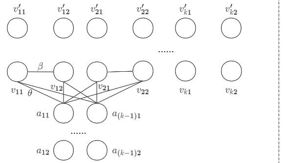
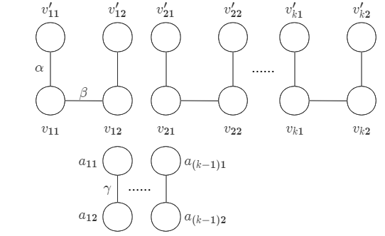
We show that the analysis in Theorem 4.4 is asymptotically tight. Consider the example as shown in Figure 6. Let $k>4$ be a constant. Denote by $\alpha_{ij},i\in[k],j\in[2]$ the edge between node $v_{ij}$ and node $v^{\prime}_{ij}$ , $\beta_{i},i\in[k]$ the edge between node $v_{i1}$ and $v_{i2}$ , $\gamma_{i},i\in[k-1]$ the edge between node $a_{i1}$ and $a_{i2}$ . Let $\theta_{i1},\theta_{i2},\theta_{i3},\theta_{i4},i\in[k]$ be the edge between node $a_{i1}$ and node $v_{11}$ , $a_{i1}$ and node $v_{12}$ , $a_{i1}$ and node $v_{21}$ , $a_{i1}$ and node $v_{22}$ , respectively. Obviously, allocating all the nodes to agent $2$ and allocating nothing to agent $1$ result in the optimal social welfare, i.e.,

\mathsf{sw}^{*}=u_{2}(V)=\sum\limits_{i\in[k],j\in[2]}w_{2}(\alpha_{ij})+\sum\limits_{i\in[k-1]}w_{2}(\gamma_{i})=3k-1.

(1)

The corresponding maximum matching $M^{*}$ contains $2k$ edges $\alpha_{ij},i\in[k],j\in[2]$ and $k-1$ edges $\gamma_{i},i\in[k-1]$ . Now, we consider the worst case achieved by Algorithm 4 running on this example, which results in a total utility of $k+3$ . In the first two rounds of the while loop in Step 5, each agent picks exactly one of the two edges $\beta_{1}$ and $\beta_{2}$ (w.l.o.g. agent 1 picks $\beta_{1}$ and agent 2 picks $\beta_{2}$ ). Following that agent $2$ picks all the remaining edges $\beta_{i},i\in[3,k]$ and arbitrary two edges $\gamma_{i},i\in[k-1]$ (w.l.o.g. $\gamma_{1}$ and $\gamma_{2}$ ). We then move out of the while loop since (1) for agent 1, $u_{1}(P)=0$ ; (2) for agent 2, $u_{2}(P)<u_{2}(X_{2})$ and allocating any other edge $\gamma_{i},i\in[3,k-1]$ to it will break EF1. Thus, we execute the envy-cycle elimination procedure on the remaining items, i.e., allocating all the remaining vertices in $P$ to agent $1$ with the EF1 allocation being completed. For agent 2, the maximum matching in $G[X_{2}]$ containing edges $\beta_{i},i\in[2,k]$ , $\gamma_{i},i\in[2]$ . We thus have $u_{2}(X_{2})=k-1+2=k+1$ . For agent 1, the maximum matching in $G[X_{1}]$ contains edges $a_{11}$ and $a_{12}$ . Therefore, $u_{1}(X_{1})=2$ . The total social welfare is $u_{1}(X_{1})+u_{2}(X_{2})=k+1+2=k+3$ . Thus

\lim\limits_{k\rightarrow+\infty}\frac{k+3}{3k-1}=\frac{1}{3},

which completes the proof of the theorem. ∎

4.3 Two Heterogeneous Agents

We then discuss the case of two agents, and show that Algorithm 5 ensures at least 1/3 fraction of the optimal social welfare. Intuitively, in Algorithm 5, we first check whether there is a single edge $e$ for which some agent $i$ has value at least $1/3\cdot\mathsf{sw}^{*}(\mathcal{I})$ . If so, allocating $e$ to $i$ already ensures $1/3\cdot\mathsf{sw}^{*}(\mathcal{I})$ . Moreover, this partial allocation is EF1 since the removal of one item in $e$ results in no edges, and thus we can use the envy-cycle elimination algorithm to allocate the remaining vertices, which returns an EF1 allocation and can only increase the social welfare. Otherwise, we compute a social welfare maximizing allocation $(M_{1},M_{2})$ , i.e., $u_{1}(M_{1})+u_{2}(M_{2})=\mathsf{sw}^{*}(\mathcal{I})$ . Without loss of generality, assume $u_{1}(M_{1})\leq u_{2}(M_{2})$ . We temporarily allocate $M_{i}$ to agent $i$ for $i=1,2$ . If the allocation is not EF1, since $u_{1}(M_{1})\leq u_{2}(M_{2})$ , it can only be the case that agent 1 envies agent 2 but agent 2 does not envy agent 1. Then we move items in agent 2’s bundle one by one to agent 1. It can be shown that there must be a time after which the allocation is EF1, and the first time when the allocation becomes EF1, the resulting social welfare is at least $1/3\cdot\mathsf{sw}^{*}(\mathcal{I})$ . Interestingly, despite the simplicity of Algorithm 5, we can show that no algorithm that has better than 1/3 approximation. Formally, we have the following theorem.

Theorem 4.7.

For any instance $\mathcal{I}$ with two heterogeneous agents, Algorithm 5 returns an EF1 allocation with social welfare at least $1/3\cdot\mathsf{sw}^{*}(\mathcal{I})$ , which is optimal.

0: Instance

\mathcal{I}=(G,N,\mathbf{w})

with

G=(V,E)

0: Allocation

\mathbf{X}=(X_{1},X_{2})

1: if there is

e\in E

such that

w_{i}(e)\geq 1/3\cdot\mathsf{sw}^{*}(\mathcal{I})

for some

i=1,2

then

2: Assign

e

to agent

i

and run envy-cycle elimination algorithm for the vertices.

3: else

4: Computing a social welfare maximizing allocation

(M_{1},M_{2})

. Without loss of generality, assume

u_{1}(M_{1})\leq u_{2}(M_{2})

, and assign

M_{i}

to agent

i

for

i=1,2

5: while agent

1

envies agent

2

for more than one item do

6: Reallocate some item

v\in X_{2}

to agent

1

, i.e.,

X_{2}\leftarrow X_{2}\setminus\{v\}

and

X_{1}\leftarrow X_{1}\cup\{v\}

7: end while

8: end if

9: Return the allocation

(X_{1},\cdots,X_{n})

Algorithm 5 EF1 Allocation with tight social welfare guarantee for 2 Heterogeneous Agents

Proof.

Denote $(M_{1},M_{2})$ as a social welfare maximizing allocation. Consider the following two cases:

•

Case 1: $\exists e\in E$ such that $w_{i}(e)\geq\frac{1}{3}\cdot\mathsf{sw}^{*},i\in\{1,2\}$ ;
•

Case 2: $\forall e\in E$ , $w_{i}(e)<\frac{1}{3}\cdot\mathsf{sw}^{*},i\in\{1,2\}$ .

For Case 1, giving edge $e$ to agent $i$ and running the envy-cycle elimination procedure on remaining vertices can find an EF1 allocation, which, at the same time, guarantees the total utility no less than $1/3$ of the maximum possible social welfare.

Next, we consider Case 2. There are two subcases.

•

Subcase 1: $u_{i}(M_{i})\geq\frac{1}{3}\cdot\mathsf{sw}^{*}$ for all $i\in\{1,2\}$ ;
•

Subcase 2: $\exists i\in\{1,2\}$ such that $u_{i}(M_{i})<\frac{1}{3}\cdot\mathsf{sw}^{*}$ .

For Subcase $1$ , if such allocation guarantees EF1, the theorem holds. Otherwise, agent $1$ envies agent $2$ since we assume $u_{1}(M_{1})\leq u_{2}(M_{2})$ . We then reallocate the item $v\in X_{2}$ to agent 1 one by one until such allocation guarantees EF1. The total utility is $u_{1}(X_{1})+u_{2}(X_{2})\geq u_{1}(M_{1})\geq(1/3)\mathsf{sw}^{*}$ . Therefore, we complete the proof for this subcase.

Consider Subcase $2$ . Without loss of generality, assume $u_{1}(M_{1})<(1/3)\mathsf{sw}^{*}$ . If allocation $(M_{1},M_{2})$ guarantees EF1, the theorem is proved. Otherwise, by the assumption that $u_{1}(M_{1})\leq u_{2}(M_{2})$ , agent $1$ envies agent $2$ more than one item. By $u_{1}(M_{1})<(1/3)\mathsf{sw}^{*}$ , we have $u_{2}(M_{2})>(2/3)\mathsf{sw}^{*}$ . Now, we consider to remove items from agent $2$ ’s bundle to agent $1$ ’s bundle. First, we sort the edges within $M_{2}$ by decreasing order according to their valuation to agent $2$ . In each iteration, we pick an edge within agent $2$ ’s bundle with largest weight and give one endpoint to agent $1$ . If the allocation still admits EF1, we give another endpoint to agent $1$ and pick another edge with the largest weight in agent $2$ ’s remaining bundle. Repeat the above procedure until agent $1$ envies agent $2$ up to exactly one item. When Algorithm 5 completes, at most one edge $e$ within $M_{2}$ is destroyed, i.e., one endpoint of $e$ is allocated to agent $1$ and the other endpoint still remains in $X_{2}$ . If $e$ is the edge with the largest weight in $M_{2}$ , we have $u_{2}(X_{2})\geq u_{2}(M_{2}\setminus\{e\})>(1/3)\mathsf{sw}^{*}$ , where the last inequality holds because $u_{2}(M_{2})>(2/3)\mathsf{sw}^{*}$ and $w_{2}(e)<(1/3)\mathsf{sw}^{*}$ . We thus complete the proof of the theorem. Otherwise, we next show that $u_{2}(X_{2})\geq(1/3)u_{2}(M_{2})$ . Let $X^{\prime}_{2}$ be the set of items given to agent $1$ . We have

w_{2}(e)\leq u_{2}(X^{\prime}_{2})\leq u_{2}(X_{2}),

(2)

where the first inequality holds because at least one edge within $M_{2}$ with larger weight is allocated to agent $1$ before and the second inequality holds since otherwise agent $2$ will envy agent $1$ . We thus derive

u_{2}(X_{2})\geq\frac{1}{3}(u_{2}(X_{2})+u_{2}(X^{\prime}_{2})+w_{2}(e))\geq\frac{1}{3}u_{2}(M_{2}).

(3)

Furthermore

$\displaystyle u_{1}(X_{1})+u_{2}(X_{2})$	$\displaystyle\geq u_{1}(M_{1})+\frac{1}{3}u_{2}(M_{2})$	(4)
	$\displaystyle\geq\mathsf{sw}^{*}-u_{2}(M_{2})+\frac{1}{3}u_{2}(M_{2})$
	$\displaystyle=\mathsf{sw}^{}-\frac{2}{3}u_{2}(M_{2})\geq\frac{1}{3}\mathsf{sw}^{},$

where the last inequality holds because $u_{2}(M_{2})\leq\mathsf{sw}^{*}$ . Since in each iteration, at most one item is removed from agent $2$ to agent $1$ , Algorithm 5 runs in $poly(|V|)$ time. We complete the proof of the theorem.

Tight Example

We next show the approximation of $1/3$ is optimal. Consider the example in Fig. 7(a) and Fig. 7(b). It is not hard to verify that the maximum social welfare without fairness constraint is $\mathsf{sw}^{*}=3$ by allocating all the items to agent 1. However, for any allocation where agent 1 has utility no smaller than 2, the allocation is not EF1 to agent 2 since agent 2 always has utility 0 in such allocations. Therefore, the maximum social welfare generated by EF1 allocations is no greater than $1+2\epsilon$ . Thus

\lim_{x\to 0}\frac{1+2\epsilon}{3}=\frac{1}{3},

(5)

which means the approximation ratio of $1/3$ is optimal. ∎

4.4 Homogeneous Agents

0: Instance

\mathcal{I}=(G,N)

with

G=(V,E;w)

0: Allocation

\mathbf{X}=(X_{1},\cdots,X_{n})

1: Find a maximum matching

M^{*}

G

. Denote by

V^{\prime}

the set of unmatched vertices by

M^{*}

2: Find the greedy partition

(M_{1},\cdots,M_{n})

of edges in

M^{*}

such that

w(M_{1})\geq\cdots\geq w(M_{n})

3: Set

X_{i}=V(M_{i})

for

i=1,\cdots,n

4: if

|M^{*}|\leq n

then

5: Let

X_{n}=V(M_{n})\cup V^{\prime}

6: Return

(X_{1},\cdots,X_{n})

7: end if

8: Construct the EF1-graph

\mathcal{G}=(N,\mathcal{E})

based on

(X_{1},\cdots,X_{n})

9: Set

Q

be the agents with positive in-degree.

10: for

i\in Q

11: Let

e_{i}=(v_{i1},v_{i2})

be the last edge added to

M_{i}

in the greedy-partition procedure.

12:

X_{i}=X_{i}\setminus\{v_{i1}\}

and

V^{\prime}=V^{\prime}\cup\{v_{i1}\}

13: end for

14: for

v\in V^{\prime}

15: Let

i=\arg\min_{i\in N}u(X_{i})

16: Set

X_{i}=X_{i}\cup\{v\}

17: end for

18: Return

(X_{1},\cdots,X_{n})

Algorithm 6 Computing EF1 Allocations with High Social Welfare for

n

Homogeneous Agents

Theorem 4.8.

For any homogeneous instance $\mathcal{I}$ , Algorithm 6 returns an EF1 allocation with social welfare at least $(2/3+2/(9n-3))\cdot\mathsf{sw}^{*}(\mathcal{I})$ in polynomial time.

In the following, we first briefly discuss the idea of Algorithm 6. We introduce the EF1-graph, inspired by the envy-graph introduced in (Lipton et al. 2004). Given a (partial) allocation $(X_{1},\cdots,X_{n})$ , we construct the corresponding EF1-graph $\mathcal{G}=(N,\mathcal{E})$ , where the nodes are agents (and thus are used interchangeably) and there is a directed edge from $i$ to $j$ if $i$ envies $j$ (or $X_{j}$ ) for more than one item,

u_{i}(X_{i})<u_{i}(X_{j}\setminus\{v\})\text{ for every $v\in X_{j}$}.

When the agents have identical utility functions, we have the following simple observation.

Observation 4.9.

The EF1-graph is acyclic; The in-degree of the agent with smallest utility is zero.

Similar with Algorithm 1, in Algorithm 6, we first compute a maximum weighted matching $M^{*}$ and let the corresponding unmatched vertices be $V^{\prime}$ . If $|M^{*}|\leq n$ , by allocating each edge in $M^{*}$ to a different agent and $V^{\prime}$ to one agent who has the smallest utility is EF1, since by removing a vertex from an edge, the remaining subgraph does not have edges any more. If $|M^{*}|>n$ , we find a greedy-partition $\Gamma(M^{*})=(M_{1},\cdots,M_{n})$ of $M^{*}$ such that $w(M_{1})\geq\cdots\geq w(M_{n})$ . However, by simply assigning $X_{i}=V(M_{i})$ for every $i$ , it may not be EF1, which is illustrated in the appendix.

To overcome this difficulty, we utilize the EF1-graph $\mathcal{G}=(N,\mathcal{E})$ on the partial allocation $(V(M_{1}),\cdots,V(M_{n}))$ . Let $Q\subseteq N$ be the set of agents who have positive in-degree, i.e., are envied by some agent for more than one item. By Observation 4.9, if $\mathcal{G}$ is nonempty, $Q\neq\emptyset$ and $n\notin Q$ . Moreover, since $M_{n}$ has the smallest weight in the greedy partition $\Gamma(M^{*})$ , $n$ has an edge to every agent in $Q$ . We first consider the partial allocation after the for loop in Step 10, which is denoted by $Y=(Y_{1},\cdots,Y_{n})$ . We can prove that $Y$ is EF1, and moreover, it ensures the desired social welfare guarantee. Finally, the remaining steps preserve the EF1ness and can only increase the social welfare of the allocation. Before proving Theorem 4.8, we first show several technical lemmas.

Lemma 4.10.

$Y$ is EF1.

Proof.

If $Q=\emptyset$ , by definition, the allocation is already EF1. In the following, assume $Q\neq\emptyset$ . Note that only the agents in $i\in Q$ has one vertex removed from $V(M_{i})$ and for any $i\notin Q$ , $Y_{i}=V(M_{i})$ . Particularly, $Y_{n}=V(M_{n})$ .

Fix any $i\in Q$ . Let $(v_{i1},v_{i2})$ be the edge selected in Step 11, i.e., the edge with the smallest weight in $M_{i}$ . By the definition of greedy partition,

\displaystyle u(V(M_{n}))\geq u(V(M_{i})\setminus\{v_{i1},v_{i2}\}).

(6)

We have the following claims.

Claim 4.11.

Agent $n$ does not envy any agent $i\in N$ for more than one item in the partial allocation $Y$ .

Proof.

The claim is straightforward if $i\notin Q$ since there is no edge between $n$ and $i$ . If $i\in Q$ , then $Y_{i}=V(M_{i})\setminus\{v_{i1}\}$ and by Inequality (6),

u(V(M_{n}))\geq u(V(M_{i})\setminus\{v_{i1},v_{i2}\})=u(Y_{i}\setminus\{v_{i2}\}),

implying $n$ does not envy $Y_{i}$ for more than one item. ∎

Claim 4.12.

No agent $i\in N$ envies agent $n$ in $Y$ .

Proof.

If $i\notin Q$ , the bundles of agent $i$ and $n$ do not change in the for loop in Step 10. Since $M_{n}$ has the smallest weight in the greedy partition of $M^{*}$ , we have

u(Y_{i})=u(V(M_{i}))\geq u(V(M_{n}))=u(Y_{n}).

If $i\in Q$ , since there is an edge from $n$ to $i$ , we have

u(Y_{i})\geq\min_{v\in V(M_{i})}u(V(M_{i})\setminus\{v\})>u(V(M_{n})),

which means $i$ does not envy $n$ . ∎

Combining Claims 4.11 and 4.12, we have that for any two agents $i$ and $j$ ,

u(Y_{i})\geq u(Y_{n})\geq u(Y_{j}\setminus\{v\})\text{ for some $v\in Y_{j}$},

which means $i$ does not envy $j$ for more than one item. This completes the proof of Lemma 4.10. ∎

To prove the approximation ratio of Algorithm 6, we need the following lemma.

Lemma 4.13.

$|M_{i}|\geq 3$ for all $i\in Q$ .

Proof.

If the in-degree of agent $i$ is non-zero, then agent $n$ must envy $i$ for more than one item, and

\displaystyle u(Y_{n})<u(V(M_{i})\setminus\{v\})\text{ for any $v\in V(M_{i})$}.

(7)

First, it is easy to see that $|M_{i}|\neq 1$ since the removal of any node $v$ makes the remaining utility be 0 and thus Equation (7) does not hold.

Next we show $|M_{i}|\neq 2$ . For the sake of contradiction, assume $M_{i}=\{e,e^{\prime}\}$ with $e=(v_{1},v_{2})$ and $e^{\prime}=(v^{\prime}_{1},v^{\prime}_{2})$ . Without loss of generality, we further assume $w(e)\geq w(e^{\prime})$ . Then it must be that $w(M_{n})\geq w(e)$ , otherwise $e^{\prime}$ cannot be added to $M_{i}$ . Note that since $M^{*}$ is a maximum weighted matching in $G$ , $\{e,e^{\prime}\}$ must be a maximum weighted matching in $G[M_{i}]$ . If there exist edges in $G[M_{i}]$ whose weights are greater than $w(e)$ , these edges must be adjacent to the same node, denoted by $\bar{v}$ ; otherwise they can form another matching with weight greater than $w(M_{i})$ . Thus by removing $\bar{v}$ from $G[M_{i}]$ , the maximum matching in the remaining graph contains at most one edge, and all the remaining edges have weight at most $w(e)$ , which means the maximum matching in $G[V(M_{i})\setminus\{\bar{v}\}]$ brings utility no larger than $w(e)$ . Therefore,

u(V(M_{i})\setminus\{\bar{v}\})\leq w(e)\leq w(M_{n}),

which is a contradiction with Equation (7). Combining the above two cases, we have $|M_{i}|\geq 3$ . ∎

Based on the claims and lemmas presented above, we present the proof of Theorem 4.8 below.

Proof of Theorem 4.8.

Let $(X_{1},\cdots,X_{n})$ be the allocation returned by Algorithm 6. If the allocation is from Step 6, then it must be EF1. This is because $X_{n}$ has the smallest value and thus nobody envies $n$ and each of $X_{i}$ with $1\leq i\leq n-1$ contains only two nodes which means the removal of one of them brings utility 0 to any agent. It also achieves the optimal social welfare since all edges in $M^{*}$ are allocated to some agents.

Next we consider the case when the allocation is obtained from Step 18. By Lemma 4.10, after the for loop in Step 10, the partial allocation is EF1. To show the final allocation to be EF1, it suffices to show that the for loop in Step 14 preserves EF1. This is true as in each round, only the bundle with the smallest value can be allocated one more item whose removal makes it smallest again.

Finally, we consider the social welfare loss. For each agent $i\in Q$ , we observe that at most one node will be removed from $V(M_{i})$ in the for loop in Step 10 and the for loop in Step 14 can only increase $i$ ’s utility. Since the removed node $v_{i1}$ is from the edge with the smallest weight in $M_{i}$ , by Lemma 4.13, we have

u(X_{i})\geq\frac{2}{3}\cdot u(V(M_{i}))\text{ for all $i\in N\setminus\{n\}$},

Moreover, for agent $n$ and any $i\neq n$ ,

\displaystyle u(X_{n})\geq u(M_{i}\setminus\{(v_{i1},v_{i2})\})\geq\frac{2}{3}\cdot u(V(M_{i})).

(8)

Therefore

	$\displaystyle\frac{\sum_{i\in N}u(X_{i})}{\mathsf{sw}^{*}}$	$\displaystyle\geq\dfrac{\sum_{i\in N\setminus\{n\}}\frac{2}{3}\cdot u(V(M_{i}))+u(V(M_{n}))}{\sum_{i\in N}u(V(M_{i}))}$
		$\displaystyle=\frac{2}{3}+\frac{1}{3}\cdot\dfrac{u(V(M_{n}))}{\sum_{i\in N}u(V(M_{i}))}$
		$\displaystyle\geq\frac{2}{3}+\frac{1}{3}\cdot\dfrac{u(V(M_{n}))}{(\frac{3}{2}(n-1)+1)\cdot u(V(M_{n}))}$
		$\displaystyle=\frac{2}{3}+\frac{2}{9n-3},$

where the second inequality is because of Inequality (8) and we complete the proof of Theorem 4.8. ∎

Tight Example.

We show that the analysis in Theorem 4.8 is asymptotically tight. Consider the example in Figure 8, where $2^{-}$ means $2-\epsilon^{2}$ and $4^{+}$ means $4+3(n-1)\epsilon^{2}$ . Let $\epsilon>0$ be a sufficiently small number, say $1/n^{2}$ . The maximum matching $M^{*}$ contains all the bold edges and $\mathsf{sw}^{*}=w(M^{*})=6(n-1)+4$ . By Algorithm 6, the greedy-partition of $M^{*}$ is $(M_{1},\cdots,M_{n})$ as shown in Figure 8. However, it is not EF1: for $1\leq i\leq n-1$ , by removing any vertex from $M_{i}$ , the maximum matching in the remaining graph has weight at least $2+\epsilon+2^{-}>4+3(n-1)\epsilon^{2}=w(M_{n})$ . After the for loop in Step 10 in Algorithm 6, for $1\leq i\leq n-1$ , one vertex in each $M_{i}$ is removed and is reallocated to $M_{n}$ in the for loop in Step 14. Thus the remaining social welfare is at most

2\cdot(2+\epsilon)\cdot(n-1)+4\to\frac{2}{3}\cdot\mathsf{sw}^{*}.

Remark.

By Theorem 4.8, if $n=2$ , the approximation ratio is 4/5 and when $n\to\infty$ the approximation ratio is 2/3. Unfortunately, we were not able to prove an upper bound where the optimal social welfare cannot be achieved by any EF1 allocation. We conjecture that there is always an EF1 allocation that achieves the optimal social welfare $\mathsf{sw}^{*}$ .

5 Conclusion and Future Directions

In this work, we study the fair (and efficient) allocation of graphical resources when the agents’ utilities are determined by the weights of the maximum matchings in the obtained subgraphs. We provide a string of algorithmic results regarding MMS and EF1, but also leave some problems open. For example, regarding MMS, we can further improve the approximation ratio when the agents are homogeneous, and prove inapproximability results; regarding EF1, the approximation ratio to the optimal social welfare for binary weight functions and homogeneous agents can be potentially improved.

Our work also uncovers some other interesting future directions. First, regarding MMS, although we show that there is no bounded multiplicative approximation, it may admit good additive or bi-factor approximations. Second, we only focus on the matching-induced utilities in this work, and it is intriguing to consider other combinatorial structures such as independent set, network flow and more. Third, we can extend the framework to the fair allocation of graphical chores when the agents have costs to complete the items, and the asymmetric situation when the agents have possibly different entitlements to the system.

References

Amanatidis et al. [2022] Georgios Amanatidis, Georgios Birmpas, Aris Filos-Ratsikas, and Alexandros A. Voudouris. Fair division of indivisible goods: A survey. CoRR, abs/2202.07551, 2022.
Aziz et al. [2022] Haris Aziz, Bo Li, Hervé Moulin, and Xiaowei Wu. Algorithmic fair allocation of indivisible items: A survey and new questions. CoRR, abs/2202.08713, 2022.
Bansal and Sviridenko [2006] Nikhil Bansal and Maxim Sviridenko. The santa claus problem. In STOC, pages 31–40, 2006.
Barketau et al. [2015] Maksim Barketau, Erwin Pesch, and Yakov M. Shafransky. Minimizing maximum weight of subsets of a maximum matching in a bipartite graph. Discret. Appl. Math., 196:4–19, 2015.
Barman and Krishnamurthy [2020] Siddharth Barman and Sanath Kumar Krishnamurthy. Approximation algorithms for maximin fair division. ACM Trans. Economics and Comput., 8(1):5:1–5:28, 2020.
Bei et al. [2021] Xiaohui Bei, Xinhang Lu, Pasin Manurangsi, and Warut Suksompong. The price of fairness for indivisible goods. Theory Comput. Syst., 65(7):1069–1093, 2021.
Bilò et al. [2019] Vittorio Bilò, Ioannis Caragiannis, Michele Flammini, Ayumi Igarashi, Gianpiero Monaco, Dominik Peters, Cosimo Vinci, and William S. Zwicker. Almost envy-free allocations with connected bundles. In ITCS, volume 124 of LIPIcs, pages 14:1–14:21. Schloss Dagstuhl - Leibniz-Zentrum für Informatik, 2019.
Bouveret et al. [2017] Sylvain Bouveret, Katarína Cechlárová, Edith Elkind, Ayumi Igarashi, and Dominik Peters. Fair division of a graph. In IJCAI, pages 135–141. ijcai.org, 2017.
Budish [2011] Eric Budish. The combinatorial assignment problem: Approximate competitive equilibrium from equal incomes. Journal of Political Economy, 119(6):1061–1103, 2011.
Buluç et al. [2016] Aydin Buluç, Henning Meyerhenke, Ilya Safro, Peter Sanders, and Christian Schulz. Recent advances in graph partitioning. In Algorithm Engineering, volume 9220 of Lecture Notes in Computer Science, pages 117–158. 2016.
Crouch and Mazur [2001] Catherine H Crouch and Eric Mazur. Peer instruction: Ten years of experience and results. American journal of physics, 69(9):970–977, 2001.
Farbstein and Levin [2015] Boaz Farbstein and Asaf Levin. Min-max cover of a graph with a small number of parts. Discret. Optim., 16:51–61, 2015.
Flanigan et al. [2021] Bailey Flanigan, Paul Gölz, Anupam Gupta, Brett Hennig, and Ariel D Procaccia. Fair algorithms for selecting citizens’ assemblies. Nature, pages 1–5, 2021.
Foley [1967] D. K. Foley. Resource Allocation and the Public Sector. Yale Econ. Essays, 7, 1967.
Garg and Taki [2021] Jugal Garg and Setareh Taki. An improved approximation algorithm for maximin shares. Artificial Intelligence, 300, 2021.
Ghodsi et al. [2018] Mohammad Ghodsi, Mohammad Taghi Hajiaghayi, Masoud Seddighin, Saeed Seddighin, and Hadi Yami. Fair allocation of indivisible goods: Improvements and generalizations. In EC, pages 539–556, 2018.
Goldman and Procaccia [2014] Jonathan R. Goldman and Ariel D. Procaccia. Spliddit: unleashing fair division algorithms. SIGecom Exch., 13(2):41–46, 2014.
Igarashi and Peters [2019] Ayumi Igarashi and Dominik Peters. Pareto-optimal allocation of indivisible goods with connectivity constraints. In AAAI, pages 2045–2052. AAAI Press, 2019.
Khani and Salavatipour [2014] M. Reza Khani and Mohammad R. Salavatipour. Improved approximation algorithms for the min-max tree cover and bounded tree cover problems. Algorithmica, 69(2):443–460, 2014.
Koç et al. [2016] Çagri Koç, Tolga Bektas, Ola Jabali, and Gilbert Laporte. Thirty years of heterogeneous vehicle routing. Eur. J. Oper. Res., 249(1):1–21, 2016.
Kress et al. [2015] Dominik Kress, Sebastian Meiswinkel, and Erwin Pesch. The partitioning min-max weighted matching problem. Eur. J. Oper. Res., 247(3):745–754, 2015.
Kurokawa et al. [2018] D. Kurokawa, A. Procaccia, and J. Wang. Fair enough: Guaranteeing approximate maximin shares. Journal of the ACM, 65(2):8, 2018.
Lipton et al. [2004] Richard J. Lipton, Evangelos Markakis, Elchanan Mossel, and Amin Saberi. On approximately fair allocations of indivisible goods. In EC, pages 125–131. ACM, 2004.
Lovász and Plummer [2009] László Lovász and Michael D Plummer. Matching theory, volume 367. American Mathematical Soc., 2009.
Miyazawa et al. [2021] Flávio Keidi Miyazawa, Phablo F. S. Moura, Matheus J. Ota, and Yoshiko Wakabayashi. Partitioning a graph into balanced connected classes: Formulations, separation and experiments. Eur. J. Oper. Res., 293(3):826–836, 2021.
Moulin [2003] Hervé Moulin. Fair division and collective welfare. MIT Press, 2003.
Rathinam et al. [2020] Sivakumar Rathinam, R. Ravi, J. Bae, and Kaarthik Sundar. Primal-dual 2-approximation algorithm for the monotonic multiple depot heterogeneous traveling salesman problem. In SWAT, volume 162 of LIPIcs, pages 33:1–33:13, 2020.
Suksompong [2019] Warut Suksompong. Fairly allocating contiguous blocks of indivisible items. Discret. Appl. Math., 260:227–236, 2019.
Suksompong [2021] Warut Suksompong. Constraints in fair division. SIGecom Exch., 19(2):46–61, 2021.
Traub and Tröbst [2020] Vera Traub and Thorben Tröbst. A fast (2 + 2/7)-approximation algorithm for capacitated cycle covering. In IPCO, pages 391–404. Springer, 2020.
Yaman [2006] Hande Yaman. Formulations and valid inequalities for the heterogeneous vehicle routing problem. Math. Program., 106(2):365–390, 2006.

Fair Graphical Resource Allocation with Matching-Induced Utilities

Abstract

1 Introduction

1.1 A Summary of Results

1.2 Related Works

2 Preliminaries

Definition 2.1 (α\alpha-MMS).

Definition 2.2 (EF1).

3 MMS Fair Allocations

3.1 Heterogeneous Agents

Theorem 3.1.

Proof.

3.2 Homogeneous Agents

Theorem 3.2.

Greedy Partition.

Lemma 3.3.

Proof.

Lemma 3.4.

Proof.

Lemma 3.5.

Proof.

Proof of Theorem 3.2.

Claim 3.6.

Proof.

Theorem 3.7.

Proof.

Lemma 3.8.

Proof.

4 EF1 Allocations

4.1 General Heterogeneous Agents

Theorem 4.1.

Proof.

Theorem 4.2.

Lemma 4.3.

Proof.

Proof of Theorem 4.2.

4.2 Binary Weight Functions

Theorem 4.4.

Lemma 4.5.

Proof.

Lemma 4.6.

Proof.

Proof of Theorem 4.4.

Tight Example.

4.3 Two Heterogeneous Agents

Theorem 4.7.

Proof.

Tight Example

4.4 Homogeneous Agents

Theorem 4.8.

Observation 4.9.

Lemma 4.10.

Proof.

Claim 4.11.

Proof.

Claim 4.12.

Proof.

Lemma 4.13.

Proof.

Proof of Theorem 4.8.

Tight Example.

Remark.

5 Conclusion and Future Directions

References

Fair Graphical Resource Allocation with
Matching-Induced Utilities

Definition 2.1 ( $\alpha$ -MMS).