On the Fast Track: Rapid construction of stellar stream paths2022On the Fast Track: Rapid construction of stellar stream paths–A
Abstract
Stellar streams are sensitive probes of the Galactic potential. The likelihood of a stream model given stream data is often assessed using simulations. However, comparing to simulations is challenging when even the stream paths can be hard to quantify. Here we present a novel application of Self-Organizing Maps and first-order Kalman Filters to reconstruct a stream’s path, propagating measurement errors and data sparsity into the stream path uncertainty. The technique is Galactic-model independent, non-parametric, and works on phase-wrapped streams. With this technique, we can uniformly analyze and compare data with simulations, enabling both comparison of simulation techniques and ensemble analysis with stream tracks of many stellar streams. Our method is implemented in the public Python package TrackStream, available at https://github.com/nstarman/trackstream.
Keywords:
Astrophysics - Astrophysics of Galaxies – Galaxy: structure – Galaxy: kinematics and dynamics – methods: data analysis – methods: statistical1 Introduction
A stellar stream is the association of stars tidally stripped from a common progenitor system that orbits in an underlying galactic gravitational field (Johnston 1998; Helmi & White 1999). Stream progenitors are gravitationally bound systems, such as satellite dwarf galaxies or star clusters (Odenkirchen et al. 2001; Majewski et al. 2003). In the absence of external interactions these systems are stable, though still capable of mass loss driven by internal processes (Hills 1975; Heggie & Hut 2003), e.g. relaxation and binary interactions. Considering external interactions, these progenitor systems may be disrupted: completely, as in the merger events that formed the Galactic stellar halo (Lynden-Bell 1967; Searle & Zinn 1978); or partially, such as tidal disruption forming a stellar stream.
In the approximation of a smooth galactic gravitational field, the progenitor’s extent is limited to the tidal radius. Through processes internal and external, progenitor stars can achieve sufficient energy to bring them beyond the tidal boundary, thus “escaping” into the galactic field. Escape primarily occurs at both an inner and outer saddle point of the combined potential – e.g. the L2 and L3 Lagrange points for a spherical galactic field (Ross et al. 1997; Fukushige & Heggie 2000; Binney & Tremaine 2008). Generally, the initial phase space position of the escaped star is very similar to that of the progenitor: the configuration position is the tidal boundary and the star has a low peculiar velocity. Since both the escaped star and its progenitor orbit in the same underlying galactic potential and have similar phase space positions their orbits are similar (Binney & Tremaine 2008). Given sufficient time the phase space separation will increase and an escaped star will lead or trail the position of the progenitor, depending on the location from which it escaped. Therefore, a collection of tidally stripped stars will form extended structures, aka tails or streams, that are few to thousands of parsecs in length (Johnston 1998; Helmi & White 1999; Bovy 2014).
To be a coherent, observable structure the peculiar velocity dispersion of escaped stars relative to the progenitor must be relatively low, but does vary from system to system. Stars in kinematically hot streams (e.g. from progenitors with larger kinematic dispersions) have more dissimilar orbits from each other and the progenitor than do stars in cold streams, with smaller dispersions (Johnston 1998; Hendel & Johnston 2015). The orbit of a star depends on its phase space position and the gravitational potential; therefore measuring a star’s position and velocity and observing its orbit reveals the local potential, which is normally dominated by the Galaxy (primarily the dark matter halo at large distances) (Gibbons et al. 2014). However, an orbit is impractical to observe on human timescales. Cold streams offer a workaround. Like measuring one star at many points in one orbit over an extended period, streams are many stars measured at different points along approximately one orbit at the same time. Therefore stellar streams are one of the most promising means to study the Galactic gravitational potential: the stellar components as well as the dark matter (Johnston 2016).
On the observational front there has been a large concerted effort in the field to find new stellar streams (Mateu 2022, for an extensive list of known Galactic streams see), extend the detected extents of known streams (Rockosi et al. 2002; Ibata et al. 2017; Grillmair & Dionatos 2006; Carlberg et al. 2012; Starkman et al. 2019, e.g. for Palomar 5 alone:), and increase the general purity of stream catalogs. On the simulation end, there are numerous methods to generate and model stellar streams, spanning many degrees of complexity. The simplest method is modeling the stream as tracers sampled from a single orbit, a technique called orbit fitting (Johnston et al. 1999; Malhan & Ibata 2019, e.g.). However, streams generally do not lie on a single orbit (Sanders & Binney 2013) and this approximation can produce biased results. The distribution function method of Bovy 2014 starts from the orbit of the progenitor, but also models the mean difference between the stream’s and progenitor’s orbits. Like orbit fitting, this method produces an analytic characterization of the stream’s trajectory, albeit in action-angle coordinates that are converted to a phase-space track by linear interpolation. The distribution function method is a marked improvement over the orbit approximation, however it makes a number of simplifying assumptions and also struggles to model interactions with the stream that can perturb the path. Particle spray models (Fardal et al. 2015; Bonaca et al. 2014, e.g.) redress some of these shortcomings by integrating orbits of many tracer particles released over time from a simulated progenitor. Models of tidal disruption and interactions can be explored in this framework. However, particle spray methods are non-analytic and are also more computationally intensive than their analytic counterparts. The most expensive, but also most accurate and detailed, stream modeling method is direct -body simulation simulations, e.g. bespoke modeling of GD-1 to try to identify the progenitor (Webb & Bovy 2019).
How observations and simulations are compared depends on the simulation method. When using analytic methods like distribution functions (Bovy 2014) this comparison can unsurprisingly be done analytically, by directly modelling the mean path, width, and other properties along the stream. Computing fit statistics to real data is straightforward in this framework. For non-analytic simulation methods, where the stream is modeled by a set of tracer particles, a direct comparison to data is challenging. One method, from Bonaca et al. 2014, is to calculate probabilities for each tracer and marginalize over all model points. For a smooth likelihood function this method requires several times more model points than data points, and is a notable limitation when trying to closely match observations, e.g. with an N-body simulation. Thus, this method is well-suited for its intended use case, less so for other situations. A different and common approach to analyzing streams, both in simulations and from observations, is by fitting a stream track: a smooth path through phase space which characterizes the trajectory of the stream. For visualization, checking the sky footprint, and calculating model likelihoods the track of a stream is a multi-purpose tool. In many respects, what is meant by a stellar stream is its track, not its constituent stars.
Despite its centrality to the field, there is no set definition and a multitude of computational methods for defining a stream track. The most common definition of a stream track is with a low order polynomial fit. The stream is projected from its initial reference frame, e.g. ICRS (Arias et al. 1997), into a rotated on-sky frame, with longitude and latitude , such that the stream extends along . In this frame the stream may be fit by a low-order polynomial as a function of (Bonaca et al. 2020, e.g.). Similar, if more sophisticated, methods swap tools like univariate splines (Erkal et al. 2017; Bonaca & Hogg 2018, e.g.) for the low-order polynomials. Using a coordinate dimension, here , as the independent variable works for many streams, as sweeps monotonically along the stream. For example GD-1 is straight for over 80 degrees (Webb & Bovy 2019; Price-Whelan & Bonaca 2018). However, this is not true in general: a stream’s path can become kinked by subhalo interactions, or curved on the celestial sphere in an observer’s reference frame, or like the Magellanic stream wrap multiple times around the Milky Way (Wannier & Wrixon 1972). When a stream track is not a function, methods fitting fail. One solution is to instead fit in both and non-parametrically, for example using 2-D splines (Erkal et al. 2017; Koposov et al. 2019; Li et al. 2021; Tavangar et al. 2022). This method allows for the path, width, and numerous other properties to be fit simultaneously. Though implemented in 2-D, the method is extensible to higher dimensions and so can be used, e.g. with full 3-D measurements from Gaia or simulations. While powerful, this technique is slow, requiring Monte Carlo methods to optimize the number and placement of the spline nodes. Given its speed constraints, the method cannot be reasonably used as a step in a larger Monte Carlo analysis, such as to derive stream tracks for the generative stream models discussed previously.
In order to compare simulations to data as a step in a Monte Carlo analysis we require a fast method to derive stream tracks. Without the opportunity to examine each step, the method must work when the stream track is not a one-to-one function, such as with phase wraps. We require the method to work on data with errors, constrained to be on-sky or in full 3-D, and with and without velocities. Furthermore, the same method should work on many different mock stream generation methods – including analytic, particle sprays, and -body simulation simulations – so that results derived with one simulation technique can be compared to the results from another. In this paper we present a novel method for accomplishing these goals: rapidly constructing stellar stream tracks, accounting for measurement error and data sparsity. The technique is Galaxy-model independent, non-parametric, and works on many different mock stream generation methods. Our method is implemented in the public Python package TrackStream, available at https://github.com/nstarman/trackstream.
The organization of this paper is as follows. In Section 2 we present a sequence of methods for ordering the stars in a stellar stream. This order will allow us to treat the data similarly to a time-ordered data set, and therefore apply time-series techniques to reconstruct the stream track. In Section 3 we present one such application – the Kalman Filter. In Section 4 we apply the stream track pipeline to a variety of data. We conclude with discussion in Section 5.
2 Methods: Ordering the Data
The first step in the stream path fitting procedure is ordering the data. With simulated data, there are numerous options for ordering, such as the ejection time from the progenitor (Gibbons et al. 2014) or in action-angle coordinates (Bovy 2014). However real observations rarely, if ever, permit these orderings. Instead we order using only configuration and kinematic phase-space information.
Consider the toy model of a static, spherical potential (for both the Galaxy and progenitor) where all test masses (stars) are ejected with the same velocity. As the progenitor orbits the Galactic COM, its orbital path describes an elliptical path in an orbital plane. The progenitor’s tidal tails (stream) will likewise lie near the progenitor’s orbital plane. Observing from the Galactic center, an orbital plane lies on a great circle in the observer’s ‘sky’ and it is possible to re-orient the longitude () and latitude () to a stream-oriented coordinate system () with the progenitor at the origin and the stream along . However, our observations are not from the Galactic center, but approximately 8 kpc distant (GRAVITY Collaboration et al. 2018; Leung et al. 2022, for recent measurements, see). For an arbitrary stream lying (approximately) along a galactocentric ellipse there is no guaranteed rotation to “linearize” the stream in the observer coordinates so that the stream lies along . Thankfully, many streams are sufficiently distant from both the Galaxy and observer or oriented such that a rotation a) exists, or b) applies to significant lengths of the stream before deviations become problematic. When modeling streams and fitting a track in the same representation as the data, for most streams transforming to the stream-oriented coordinate system is a worthwhile first step to ordering the data and is discussed in Section 2.1.
The second step takes advantage of the low-dimensional structure of streams. Spatially, streams are approximately 1-dimensional curves in a 2-to-6 dimensional space (depending on the number of available phase-space dimensions). Rather than constructing a data-ordering in real (e.g. position and velocity) space, we can instead find a 1-D subspace in which the stream is approximately a line, and the ordering is more evident. Following Section 2.1, in Section 2.2 we describe a robust and performant means to recover an approximate 1-D subspace containing the stream and then order the stream data.
2.1 Great-Circle Coordinate Frame
Constructing the stream-oriented coordinate system requires three parameters, a new on-sky origin – at longitude and latitude – and a rotation angle about the origin. The new origin point is chosen to be the location of the progenitor, if known, and anywhere reasonable on the stream otherwise. In simulations the location of the progenitor is always known, even if the progenitor has fully dissolved. The rotation angle must be fit. Since errors in , are negligible in both (contemporary) observations and simulations, the best-fit parameters are found by simple ensemble minimization of of the stream stars. For the fixed origin point (, ) on the sky and rotation , the transformation11 1 In TrackStream, the rotation transformation is implemented to be consistent with astropy’s SkyOffsetFrame and the resulting frame can be used with the astropy package (Astropy Collaboration et al. 2022). to a stream-oriented great-circle frame () is given in a Cartesian basis by (Bovy 2011):
| (1) | ||||
Figure 1shows an example construction of a rotated reference frame for a mock stream of NGC 5466 (El-Falou & Webb 2022). The mock stream was simulated with the particle-spray code streamspraydf (Qian et al. 2022), now found in galpy (Bovy 2015) but originally from streamtools (Banik & Bovy 2019), which is an implementation of the Fardal et al. 2015 method. The current position and velocity of the progenitor globular cluster is from Vasiliev 2019. The initial conditions (the progenitor before it is disrupted and forms tidal tails) are set by back-integrating the current phase-space position 5 Gyr in MWPotential2014 (Bovy 2015): a good approximation of the Galactic potential (Bovy et al. 2016) composed of a linear combination of a spherical potential from a power-law density with an exponential cut-off Galactic bulge, an NFW dark matter halo (Navarro et al. 1996), and a Miyamoto & Nagai 1975 disc. The initial progenitor is forward integrated in the same potential, forming the tidal tails shown in the top panel of Figure 1.
The stream-specific coordinate frame is the first step to ordering the data along the stream’s path. Depending on the stream and projection effects, ordering by might be close (or quite far) to this correct ordering. Generally, ordering by is excellent for , and progressively worse at larger . Figure 1 demonstrates the usefulness of constructing a stream-specific reference frame: in ICRS coordinates the Declination is not a one-to-one function of the Right Ascension , but the middle sub-figure shows the stream is very well ordered by . Better yet, since NGC-5466 is reasonably thin and straight (in projection), the ordering remains valid for the full observed length of the NGC-5466 mock stream.
For long streams that wrap around the sky (called phase wrapping) or that curve such that is not one-to-one, this ordering fails without further intervention. While this failure does not quite happen with Figure 1, extrapolating from NGC-5466, at projection effects will ruin the simple -ordering approach. In general, streams cannot be ordered well by their longitude coordinate. We require a coordinate that better tracks the structure of the stream. Looking at Figure 1, finding the on-track coordinate is somewhat analogous to deforming the dimension, wrapping it to meet the curvature of the stream. Another way of understanding the transformation is to consider again a galactocentric great circle. Intuitively we see that such an arc only projects to a line for an observer on the plane of the great circle. For all other locations, only a non-linear projection is guaranteed to map the curve to a line. In essence, the non-linearity of the projection encodes the spatial components of the galactocentric-to-observer reference frame transformation. We note, however, that this approach cannot easily be reverse engineered to provide a novel measure of the galactocentric frame parameters. Next we describe how we can find a non-linear projection to recover the 1-D subspace of a stream and use the on-stream coordinate to order the data.
2.2 Self-Organizing Maps
To determine a stream’s 1-D subspace we use the simple neural network method of Self-Organizing Maps (SOMs). SOMs are primarily for low-dimensional, discrete representations of data. Using prototype vectors linked in a lattice structure of a desired topology, SOMs approximate the data by iteratively updating the prototypes to approximate the data distribution. In final form, each prototype maps nearby high-dimensional data to a lower-dimensional lattice. For a detailed discussion we refer the reader to Calvetti & Somersalo 2021.
2.2.1 The Algorithm, in 1-D.
Here we review the standard SOM algorithm and mathematics as they apply to a reduction from the higher-dimensional phase space of the positions (and velocities) to a one-dimensional subspace. The SOM can be extended to arbitrary features, perhaps to include photometric information, but we defer that for future work.
The data consists of tracers measured at positions in the -dimensional phase-space. In simulations, streams are generally best represented in galactocentric Cartesian coordinates, but observations are taken in spherical coordinates: two angular positions, possibly a radial distance, and corresponding kinematics. An important part of the SOM is the data-space distance metric, which is a complication when working in Cartesian coordinates versus on the surface of a sphere. For spherical coordinates the correct distance metric is the Vincenty 1975 formula; this is used in TrackStream and the figures in this paper. For many streams the angular separation between tracers is small, so it is reasonable to work within a flat sky approximation and simplify to a Euclidean distance metric in Cartesian coordinates. Therefore, for simplicity here we only discuss the method in Cartesian coordinates.
The SOM will learn the structure of the data using a smaller number of “prototype” vectors in the same space as the data. The need for only a few prototype vectors is analogous to how only two points are required to describe a line, no matter how many data points are sampled from the line. The relationship between the prototype vectors determines the topology and ordering of the data . Returning to the line example, the relationship between the two line points is a linear segment, so when fit to a dataset drawn from a line distribution, the SOM should describe the data well.
Generically the prototypes’ relationships are described with a feature map , where each prototype has a corresponding lattice node . However, since streams are one-dimensional the only pertinent information is the index: . encodes that prototypes , are neighbors if and only if the corresponding lattice points , are neighbors – i.e. .
With this review of feature and lattice space we are ready for the SOM algorithm:
- (1):
Given the data in the stream coordinates (Section 2.1),
- (2):
Choose prototypes with linear lattice .
- (3):
Iteratively,
- (1):
Select the next datum .
- (2):
Update the data-space position of the nearest prototype, keeping the lattice unchanged.
- (3):
Similarly update all the prototypes’ topological (lattice) neighbors, making smaller updates for more distant prototypes.
- (1):
By multiple iterations the prototypes will be updated to lie near the data in position space and capture the structure of the data in lattice space. For a more mathematically detailed explanation see Appendix A and TrackStream for a code implementation.
2.2.2 Projecting on the SOM
After applying the SOM and deriving the set of prototype vectors, the next step is to project the data into the 1-D space and order the data in a manner consistent with the topology. There are numerous projection algorithms, such as U-matrix maps (Ultsch & Siemon 1990), that are intended for clustering data by the lattice-point distance. The is not of interest; we want to project on the real-space structure of the SOM, and so implement a custom algorithm to connect and project onto the SOM prototypes. While it is tempting to connect the SOM prototypes with a smooth curve, e.g. a Bezier curve (Bezier 1982) or 3rd order piece-wise polynomial spline, not only is projection onto a curve challenging, it is not correct for an SOM with a linear lattice. The SOM topology is a linear structure and the SOM prototypes are connected by line segments. Projecting each datum reduces to the task of 1) identifying the correct line segment and 2) projecting onto that segment.
The custom algorithm, with examples drawn from Figure 2, is as follows:
- (1):
Get the ordered lattice points (black) from the SOM. The first point is the nearest to the specified origin (e.g. the stream progenitor, see Section 2.1 for details) and subsequent points draw their ordering from the topology.
- (2):
Compute the directed real-space segments from one lattice point to the next.
- (3):
For each data point, compute the real-space projection onto each segment
(2) (3) for data point , and lattice points . Projections between the two lattice points have .
- (4):
For each data point, compare the distance to each node and to each projection to find which node / segment it should be associated with.
- (1):
data with are closest to a node.
- (2):
data with projection parameter will be closer to that projection than any node (e.g. ) and can be distinguished between segments by the point-to-projected-point distance. E.g., data point (green) is closer to projected point than to and therefore belongs in the - segment.
- (3):
data with or and that are closest to a lattice terminal node are within the “end-caps”, e.g, .
- (4):
data with or and not in an end-cap are in a convexity, e.g, .
- (1):
- (5):
Within each “block” (end-cap, segment, convexity) organize the associated data points:
- (a)
data in an end-cap are organized by distance along the projection (extending ).
- (b)
data in a segment are ordered by .
- (c)
data in a convexity are ordered by their angular coordinate sweeping from one segment to the next. This is why precedes in Figure 2.
- (a)
- (6):
Order the blocks by the lattice node ordering.
In short, the SOM is trained on the data and then used to order the data by projecting the data onto the SOM’s 1-D subspace. Standard methods to order a stream rely on the stream being a one-to-one function in an observational coordinate, for example the position angle on the sky. Figure 3 shows that SOMs are not subject to this limitation and can be used to order streams that wrap around the Milky Way or are in other ways not one-to-one functions in any observational coordinate. Figure 3 is a mock dataset of stars in a stream-like structure, created by integrating the orbital path of the sun (Reid & Brunthaler 2004; GRAVITY Collaboration et al. 2018; Drimmel & Poggio 2018; Bennett & Bovy 2019) in MWPotential2014 for 200 Myrs. Stars are drawn randomly along the “stream“ from a Gaussian distribution. The SOM prototypes are initialized using equi-frequency binning. Unlike the NGC 5466 simulation (see Figure 1), the binning produces a poor match to the data. However, after iterations (at iterations/second on a 2018 2.7GHz i7 MacBook Pro) the SOM fits well and orders the data well. Note that most of the trained SOM prototypes do not lie directly on the mock stream. For a tight curve like this one, the offset is expected: points near to a prototype influence its location, so prototypes are generally interior to a convexity as that is locally the best average position.


Figure 4shows the SOM-derived order for a simpler example, the mock NGC-5466 stream also shown in previous figures. Two SOMs are used, one for each stream arm. Each SOM is trained for 10,000 iterations ( second on a 2018 2.7GHz i7 MacBook Pro). The prototypes cluster more densely where the data are dense, such as in the right-hand arm, but still provide good coverage of the whole stream. Shown by the colormap, the SOM order is good, with stars near in position likewise near in the ordering. For this stream the SOM is not strictly required as the position angle is sufficient to order the data. The SOM can be initialized with random prototypes and a connecting lattice, or with an informed guess. Given enough iterations both will typically converge to the same solution, but the former will require many more iterations than the latter. Rather than skipping the SOM step, we instead use an informed initial condition22 2 In TrackStream any initialization may be used. If none is specified the code defaults to equi-frequency binning, placing the a prototype at the average location of every th set of data points, where is the number of data divided by the number of prototypes. Equi-frequency binning equitably spreads the prototypes over the data, if the data is one-to-many in . If the data is many-to-one in , for example with phase-wrappings, the binning is poor.and reduce the training iterations, e.g. only the 10,000 used here. For Figure 4 the SOM prototypes are initialized by equi-frequency binning in .
Were NGC-5466 simulated again in a slightly perturbed potential or with similar initial conditions, the stream would be generally similar. A SOM trained on the previous simulation can be the initial condition for the SOM of the new simulation, therefore requiring very few iterations to converge and match the new simulation. Re-using an SOM for a similar simulation is a technique that works for any stream, but is particularly useful for complex streams, for example Sagittarius which wraps several times around the Galaxy (Koposov et al. 2012). Consider a generative model run as part of a likelihood calculation in a Markov Chain Monte Carlo (MCMC). Steps in the MCMC are to nearby points in the parameter space of a potential and progenitor, and as discussed in the context of NGC-5466, the generated mock stream will be similar to the previous stream. For the initial state of the MCMC the SOM must either run for many iterations or have an informed starting point. For subsequent steps, the previous SOM may be used as an informed starting point and should require only a little tuning, not wholesale retraining. Generally, we expect the generative model of the stream to be the time-limiting portion of any pipeline, not the SOM.
3 Methods: Constructing Stream Track by Kalman Filter
Cold streams are approximately 1-D and using a SOM we have shown that stream data can be projected into a subspace that is better suited for ordering than on-sky coordinates. The remaining task is to move through the ordered data, fitting the track, width, and any other observables along the stream. We will be using a first-order Newtonian Kalman filter to fit the phase-space track. Before deriving how Kalman filters work, it is beneficial to take a step back and outline the challenges of the data and take stock of alternative approaches.
The data are comprised of observations (real or simulated) of stars known to be members of the stream. This data has at least the on-sky position, and also perhaps the distance and kinematics of each star. Consider a dataset of only the on-sky positions. For finding the on-sky stream path it is appealing to fit with a low-order polynomial. For a sufficiently trivial stream, this approach can work. However, if the stream has any kink(s) – i.e. from interactions – or curvature – as can happen from projection into an observer’s reference frame – then the stream path might not be a function, as can be seen in Figure 3, as is required to fit a low-order polynomial.
To achieve a general solution the data cannot be fit one coordinate against another; much better is to have an affine variable and instead fit parametrically for each coordinate. For a stream, this affine parameter can be the arc-length, i.e. the angular distance along the mean path of the stream. The point-to-point distances of the data projected onto the SOM’s subspace are very nearly this arc-length. With the arc-length as the affine parameter one might do a Gaussian process regression (Cervone & Pillai 2015) or fit any manner of function: low-order polynomial, B-spline, Bezier curve. However, all these procedures are susceptible to the same problem, the SOM is an unsupervised machine learning technique and is not guaranteed to converge. In particular, if trained quickly it can make small mistakes in the ordering. In principle this shortcoming can be overcome by more training iterations, but if time is a constraint, this extra step may not be practical and may require human supervision to confirm an optimal fit, which is likewise impractical. Therefore, a general fitting procedure for stream data should on the one hand use the SOM-derived data ordering as an approximate affine variable, but also be insensitive to small inaccuracies in that ordering. A fitting method that meets both these requirements is the Kalman filter, presented here.
The Kalman filter is a well-established algorithm to estimate a joint probability distribution over unknown variables from a time series of measurements that may have statistical noise (Kalman 1960). In this context the unknown variables characterize the stream path and the measurements are the 2-to-6 astrometric dimensions of the stream’s stars.
Kalman filters fit data in a very different manner than e.g. polynomial fitting, which works by minimizing some global residual function. Instead, Kalman filters start at some initial state (a “position” in the astrometric phase-space) and sequentially introduce measurements, evolving the state and associated uncertainties according to a dynamical model of the system. This method is a two-step process. The first step is a priori: predicting from the prior state and the dynamical model the current state variables and uncertainties. The next step is a posteriori: adjusting the predicted state given the incoming measurement. The posterior state estimate is a weighted average of the prior and measurement, with the weight determined from both the prior and measurement uncertainties. A low-noise measurement against an uncertain prior will favor the measurement in the posterior state estimation, and vice versa for a noisy measurement and high-confidence prior.
One of the simplest dynamical models, and the one used in this work, is a first-order Newtonian model. In this filter states are evolved according to , where is the position of an imaginary point moving along a smooth differentiable manifold passing near the positions of the stars. Here, is a pseudo-velocity of the imaginary point. A more complex dynamical model might incorporate the Galactic potential, taking into account the acceleration field. However, incorporating the potential introduces a lot of complexity to avoid poor physics, for negligible gain. Adjacent stars on a stellar stream do not move along the same orbit, thus simply evolving the state in the potential is incorrect. For example, the streak-line model (Küpper et al. 2012) back-integrates the progenitor then forward-integrates a stream star’s orbit from its progenitor ejection time. A good dynamical model might use a similar approach for the next-state prior: back-integrate the current state to its ejection (call this ), forward integrate the progenitor for the set time step, then forward integrate an ejected star for the same . The first-order Newtonian model is computationally faster for equally good results and does not require information about the potential.
3.1 Point-to-point times
Time-series methods like the Kalman filter require a time step, however the stream data are not a time series (see Section 2): first, the observations are not of the same object, and second, the observations are not taken in any relevant time order. Despite that the data are not a true time series, we can treat the data as if it were time ordered and amenable to the Kalman filter. By using the frame-rotated (Section 2.1), SOM-ordered stream (2.2) the data are organized by distance along the as-yet-unknown stream track. Consider moving along the track, passing by each data-point with some time variable : the distance ordering is ordinally equivalent to the time ordering, index-by-index.
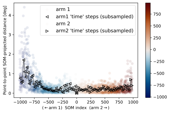
To re-interpret distances as times we take the time step as the point-to-point distance in the SOM projection of the data. For the NGC 5466 stream this distance is shown in Figure 5 as the colored points, indexed by the SOM ordering. We then smooth the time-step by kernel convolution:
| (4) |
where is the window average of the point-to-point distances in data , of window size , centered on the th index. The choice of window is arbitrary, with long-tailed windows more closely matching than short-tailed windows, which will better reflect the local density. We use a Dirichlet window (i.e. a moving window average) of window-width six – three points per side. The smoothing reduces the effects of large outliers and the result is not sensitive to larger window sizes, so this small size is kept fixed. The smoothed steps are shown as connected, directed black triangles in Figure 5. The variation in the smoothed steps is much smaller than the unsmoothed data. Now the “time”-step is tuned so that . The velocity of the Kalman Filter is not affected as we change only the time-step to make the filter accurately reach each data point.
3.2 Running the Kalman Filter
In this section we set up a Kalman filter and discuss how it is run. For a detailed review, Labbe 2021 offers an excellent discussion of Kalman filters and how to implement them in Python. Labbe 2021 works in Cartesian coordinates, but the methods are adaptable to spherical coordinates by using appropriate distance measures and being careful of angular coordinate wrappings. TrackStream supports both Cartesian and spherical metrics, which are used where appropriate for the figures. Here, for simplicity, we only present the Kalman filter math in Cartesian coordinates.
To set up a model, we assume that the stars are in a vicinity of a one-dimensional differentiable manifold following the stream track, parameterized as , where represents an artificial time, such as the scaled arc-length. Thus, the actual positions of the stars, indexed according to the SOM ordering, are given by the model
| (5) |
where is an unknown offset parameter. To link the model to observations, let denote the observed position of the th star, representing the data,
| (6) |
where is the observation error.
To set up the probabilistic phase-space model, we define an extended variable,
| (7) |
where , and is the artificial velocity vector with respect to the parameter , defined as . A local first-order Newtonian model gives us a propagation model,
| (8) | ||||
where , and and represent the approximation error in the first order model for the position and the zeroth order model for the velocity propagation, respectively.
The Equation (8)-(6) pair is written as a propagation-observation pair for the phase space variable as
| (9) | ||||
| (10) |
where the propagation-observation matrices are given by
| (11) |
and and are a unit and zero matrices, where is the number of phase-space dimensions.
The propagation-observation pair allows us to use the Kalman filtering and Kalman smoothing to estimate the parameterized manifold points . To set up a Gaussian model, we postulate that the state noise vectors and the observation noise are mutually independent and zero mean Gaussian random variables. The corresponding covariance matrices are set as
| (12) |
a commonly used form in tracking applications acknowledging the dependence of the first-order forward Euler process on the time step. The dependence that represents is the error that a smooth function can be modeled with discrete steps, using only a velocity term to update those steps. Similar to how a first-order Taylor expansion has second-order errors, the first-order Newtonian model has second-order (and higher) errors from not accounting for the smoothness. In the above formula, is a tuning parameter. For the observation error, we write
| (13) |
where accounts for the random variable represents the internal dispersion of the stars within the stream, and is the variance of the observation error.
The Kalman filtering algorithm is a sequential Bayesian filtering method, generating the conditional distribution of given all the past observations , . Under the assumption that both the model and observation noises are independent and Gaussian, the conditional distributions are also Gaussian, thus completely characterized by the conditional mean and covariance ,
| (14) |
and based on the previous state parameters and are updated in two phases, prediction step and updating (or analysis) step. The a priori prediction step is based solely on the propagation model,
| (15) | ||||
| (16) |
As the new observation arrives, the predicted distribution is considered as prior, and the update is obtained by Bayes’ formula. Writing the pre-fit residuals of the mean and covariance as
| (17) | ||||
| (18) |
the a posteriori update of the mean and covariance assume the forms
| (19) | ||||
| (20) |
where is the Kalman gain matrix,
| (21) |
The posterior state estimate is a weighted average of the prior and measurement, with the weight – the Kalman gain – determined from both the prior and measurement uncertainties. A low-noise measurement against an uncertain prior will favor the the measurement in the posterior state estimation.
The algorithm requires the initial input . To define the mean , we choose the mean position of a few stream points closest to the origin, rather than the origin itself, since streams originate at the edge of their progenitor, not their center. The initial mean velocity is the normalized mean of the differences between the first few consecutive stream points. The covariance is defined as a diagonal matrix, with the variances estimated by using the first few stream points. The approximation of as a diagonal matrix is corrected after the first time step by and later, in a back-propagation step, discussed next.
Kalman filtering, and other Bayesian filtering methods are based on the Markov models in which the next update depends on the past. When the process is run on-line, the data arriving sequentially as a time series, this updating approach is natural, while when all data are available as in the present case, no preferential direction of time can be justified. A common approach to find an estimate for the posterior distribution , , is to use Kalman smoothing, in which the filter is run in the reverse order, using the forward filtered distributions as priors. Starting with the final distribution with mean and covariance , the the Rauch-Tung-Striebel (RTS) smoother Rauch et al. 1965 algorithm walks backwards by computing the mean and covariance and through the updating formulas
| (22) | ||||
| (23) |
where the matrix back-propagates the information,
| (24) |
RTS smoothing is a powerful technique, in no small part because it helps correct for mistakes made when running the Kalman filter. An obvious correction is in the eponymous smoothing of the stream track. Also important is that the smoother will update the initial conditions , ), which are only motivated by a heuristic – a local average at the starting point. In particular the covariance should have off-diagonal terms as the measurement error is correlated in the real data. Determining good values of these initial off-diagonal terms is neither easy nor necessary as the RTS smoothing back-propagates information on the covariance from later time steps to improve .
In Figure 6 the Kalman filter pipeline is run on the SOM-ordered data from the mock NGC-5466 stream shown in prior figures. This Kalman filter was run in spherical coordinates, with the corresponding distance metric. The stream track correctly accounts for the angle wrapping at to . The track covariances (gray ellipses at time steps ) increase where the data are dense and the stream is cold and decreases elsewhere, such as as at the end-points of the stream. For most of the stream the covariance ellipses are the given width of the stream, , since the data are relatively dense and the errors in on-sky coordinates are 0 in this mock stream and negligible in, e.g. Gaia data, so do not contribute to the stream width as determined by the Kalman filter.
4 Results
Our method of fitting a track to a stream happens in three steps. First (Section 2.1) we find a reference frame to optimally represent the data. Second (Section 2.2) we find a one-dimensional subspace which approximately matches the structure of the stream and into which the stream can be projected. Third (Section 3), having ordered the data, we fit the track by Kalman filter. This three-step method produces good fits to the example data sets used thus far. In this section we show the application of the method pipeline to a variety of stellar streams, simulated using a number of different techniques.
4.1 Comparing to Distribution Function (DF) models
In Bovy 2014 stellar streams are modeled with a distribution function in action angle space. Starting from a potential, a progenitor position, and stream formation parameterization at some initial time , the initial stream distribution is evolved to time . In action-angle space the progenitor and stream is represented very simply. The action-angle stream distribution is transformed to position-momentum phase space, and similarly parameterized using linear interpolations. The DF method simulates an exact stream track and width. Figure 7 shows a mock stream of NGC 104, simulated with streamdf from Bovy 2014. The progenitor’s current phase-space position is from Vasiliev 2019 with a total disruption time 4.5 Gyr and an initial velocity dispersion of 0.365 km / s, to create a reasonably thin stream. The system is integrated in MWPotential2014 with an actionAngleIsochroneApprox to map phase space coordinates to the action-angle coordinates required by the mock-stream generator (Bovy 2015).
In contrast the TrackStream pipeline estimates the track from stream sample points (e.g. stars) in position-momentum phase space. To compare TrackStream to a DF prediction we sample from the stream, transforming from action-angles space, and run TrackStream on the sample. Figure 7 shows the result and comparison to the DF-derived stream path. For visualization we use an intrinsic stream width () of 300 pc, which exaggerates the size of the covariance ellipses. When run with the more accurate intrinsic stream width of 100 pc the two methods agree within over their lengths. The DF track extends beyond that of TrackStream since there are no tracer particles sampled at those distances. Another major difference between the two methods is what is meant by the track width. The DF analytically calculates the intrinsic width of the stream, which is a 1- Gaussian along the track. TrackStream combines an intrinsic stream width with the uncertainty in each datum point and the sparsity of the data to derive a covariance of the confidence in the track. This difference can be seen in Figure 7, especially in regions of data sparsity, like the poorly-sampled outer lengths of the stream. Here the confidence in the stream track is quite low. For a large number of well-measured data points TrackStream and the DF converge, such as near the progenitor in Figure 7.
The stream DF approach of Bovy 2014 and similar (e.g. Sanders 2014) are some of the few analytic means to simulate stellar streams. However the method is subject to a number of limitations. First, it is generally necessary in the progenitor model to model the stripping times of stars from the progenitor to a uniform distribution. This assumption is known to be false, since the mass loss rate is highest near pericenter passages. Second, these methods do not account for the progenitor’s gravitational influence on the stream. The next stream-generation method trades analyticity for the capability to address many of these limitations.
4.2 Tracking particle spray mock streams
Particle-spray (also called release) methods are a semi-analytic model of stream formation. The model requires a potential, the current phase-space position of the progenitor, the mass of the progenitor, and the period of time and rate at which the progenitor has been disrupting. To model the internal dynamics, the model also often includes a parameter for the distribution of speeds at which particles are ejected.
First the phase-space position of the progenitor is backwards integrated to the start of the disruption period. If the model accounts for mass loss, the progenitor’s current mass may also be back-integrated to the initial mass by considering the disruption rate. Next, the progenitor is forward integrated to the present, periodically releasing particles (stars) according to the disruption prescription. The particles are released on orbits from a simulation-calibrated distribution of initial positions/velocities of released particles. When fully integrated the progenitor is at its present position. Despite the name, all released particles are stream stars and should lie along the stream track, with a reasonable dispersion.
Figure 8shows a particle-spray generated mock stream with a 47 Tucanae-like progenitor. We use the particle-spray implementation – streamspraydf – that is included in galpy (v1.8+) (Bovy 2015) , which is an implementation of the Fardal et al. 2015 method that is fully described in Qian et al. 2022. The potential is MWPotential2014 from Bovy 2014; the progenitor’s orbital parameters are from Vasiliev 2019 with the mass from Marks & Kroupa 2010 (We note that streamspraydf does not incorporate mass loss, so this mass is fixed). The disruption time is 2 Gyr, chosen arbitrarily to generate a sufficiently long mock stream. All other parameters are set to the streamspraydf defaults. The stream track is fit with the TrackStream pipeline. As in Section 4.1, for visualization purposes we set the intrinsic stream width to 300 pc. Particle-spray methods do not model the stream track, so the fit quality is seen only by comparing to the tracers. The tracks for both arms correctly start at an offset from the progenitor. Though the initial state of the Kalman filter is much closer to the progenitor, the RTS smoother correctly back-propagates the information that the stream does not start at the progenitor. As expected, the uncertainty in the track is larger at the start than immediately after. While the stream tracks are smooth, they exhibit some structure at small scales due to variations in the distribution of the stream stars. The structure in the track is a balance between the information known about the stream – e.g the intrinsic width – and the actual structure of the data. If the data has sufficient structure, be it random from low-number statistics or from e.g. subhalo interactions, so too will the TrackStream stream track. It is possible to damp structure in the track by including smoothness priors. If any sources of stream perturbations are included in the simulation, such as sub-halos, then these priors would likely be quite complex. Alternatively, in simulations one can generate more tracer particles, providing more information when constructing the stream.
4.3 Tracking an -body simulation model
-body simulations are the most accurate but also computationally expensive of the stream simulation methods, making the fewest time-saving approximations. A high resolution -body simulation simulation may achieve one-to-one parity in the number of particles to number of stars in the progenitor, model the motions with dynamic time steps to resolve close interactions, and include stellar evolution. The disruption rate is determined by the the Galactic tidal field and the progenitor’s internal kinematics, not an analytic prescription. Often the high resolution of the progenitor is not matched in the potential, where it is common to instead use a purely analytic model or to also include low(er) resolution sub-halos. When trying to match observational data, an -body simulation simulation provides the most accurate representation.
Figure 9shows TrackStream applied to an -body simulation of Palomar 5. The -body simulation is taken from Starkman et al. 2019, where we searched for extended tidal features of Palomar 5. Further details of the simulations can be found in Starkman et al. 2019. In short, we use the direct -body code NBODY6 (Aarseth 2006), evolving an initial progenitor of a 100,000 star Plummer model with a half-mass radius of 10 pc. The initial mass function is from (Kroupa 2001), with a minimum and maximum stellar mass of and , respectively. We use the stellar evolution prescription of Hurley et al. 2000, with a metallicity of , and Hurley et al. 2002 for binary stars. The cluster is evolved for 12 Gyr in MWPotential2014such that the final position, velocity, mass, and mass function are comparable to the observed properties of Palomar 5 (Ibata et al. 2017; Grillmair & Smith 2001), though the simulated cluster density is higher than observed.
The progenitor particles are removed as these are not part of the stream. Likewise we remove the neutron stars and other stellar remnants. The full -body simulation simulation includes a number of particles that were ejected from the progenitor, e.g. in a close core interaction, that are not part of the stream. These non-stream members are identified by a Local Outlier Factor (LOF) calculation (Breunig et al. 2000) with a threshold of and removed. Approximately, the LOF is a local density calculation. Since the simulated stream is dense, low density regions are likely not in the stream. The distribution of LOFs calculated for each star is very strongly peaked around the typical density of the stream. Only in the extended tidal tails is the LOF of the stream approximately that of the non-stream members. In observations it is unlikely these stars would have a high stream membership probability. The exact value of the LOF threshold often makes little difference and we find the stream track determination robust.
After removing outliers, TrackStream is applied to the data. Starting near the progenitor, like for Section 4.2, the tracks for both arms are offset from the progenitor center. At each point along the stream, the RTS-smoothed Kalman filter uses information both proceeding and preceding that point to construct the track, which smoothly fits the stream data. In higher density, kinematically cold regions the width (covariance ellipses) shrink down to the prescribed stream width, which is exaggerated here to 300 pc for visualization purposes. As expected, where the stream density decreases or the stream is kinematically hotter the track confidence decreases and the covariance ellipses grow. At the extrema of each arm’s track the uncertainty is also large since there are fewer stars and because at extrema the Kalman filter only has information on one side, not both. To the Kalman filter, the start of the stream by the progenitor is also an extremum. Physically, the progenitor is not an extrema, since the other stream arm in Figure 9 is nearby and shares the progenitor as the origin. The Kalman filter could be modified to account for the presence of other stream arm, but this is probably not advisable. Theoretically, fitting the Kalman filter to each stream arm could be done as an ensemble fit, with the progenitor as a shared constraint. While this modification would reduce the extrema-associated uncertainty, it is unclear how to perform this ensemble fit without assuming information about the potential and evolution of the cluster, assumptions we purposefully avoid. Regardless, near the progenitor the star count is usually larger than elsewhere along the stream and the track certainty is correspondingly higher, mitigating the need for an ensemble fit.

4.4 Tracking Real Streams
In the previous subsections of Section 4, TrackStream was applied to mock stream data. TrackStream also works on real data. We apply the pipeline to two of the most commonly studied stellar streams: Palomar 5 and GD-1, shown in Figure 10 and Figure 11, respectively. The Palomar 5 data are a combination of data from Ibata et al. 2017 and Starkman et al. 2019. In the stream-oriented reference frame the stream stars span almost 30 degrees in longitude but only a few degrees in latitude. The data set is very small, demonstrating that TrackStream fits reasonable tracks even for stars. Like with prior examples, the confidence in the track is a mixture of the intrinsic stream width, the errors in the data, and the data sparsity. Near the ends of the track, particularly the end point at negative longitude, the covariance ellipse is much larger than elsewhere in the stream. Looking at the nearby data, two reasons for the large covariance are that the data are sparse and that the end regions have less information (a hard limit to on one side) to inform the fit. Were the data less sparse the covariance would be more similar to the covariance at the other end point. Figure 11 shows a much larger, though still small compared to e.g. the -body simulation, data set from Price-Whelan & Bonaca 2018 of GD-1. The thin stream is hand-selected in TOPCAT (Taylor 2005) to match the selection field of Price-Whelan & Bonaca 2018. The progenitor of GD-1 is unknown, so for convenience we treat the whole stream as a single stream arm, rather than a leading and trailing arm.
5 Discussion and Conclusions
In this paper we present a novel method for rapidly constructing stellar stream tracks, accounting for measurement error and data sparsity (e.g. Fig. 8). By using stream-oriented reference-frame transformations in conjunction with Self-Organizing Maps, we treat stellar-stream data as a pseudo time-series, to which first-order Kalman filters can be applied. The technique is Galactic-model independent, non-parametric, and works on many different mock stream generation methods. Owing to its speed this method is well suited to comparing simulations to data as a step in a Monte Carlo analysis.
The track-fitting procedure, implemented in TrackStream, is two or three steps, depending on if one is working in spherical coordinates. First, if in spherical coordinates we re-orient the reference frame to minimize the training time of the following step. Second, using SOMs we infer a one-dimensional subspace that approximates the structure of the target stream and orders the constituent data. Third and last, using the subspace-order we fit the track of the stream with a Kalman filter. The track-finding technique works well for a variety of stream-generation methods: distribution functions (Section 4.1), particle sprays (Section 4.2), -body simulations (Section 4.3), even real streams (Section 4.4).
In simulations, outliers can be present. In nature, contamination by background or foreground stars can also occur. TrackStream assumes that all stars are members of the stream and should therefore contribute to the track fit: the SOM will include the outliers and contamination when finding the stream’s subspace and the Kalman filter will likewise try to move the mean path towards those points. Without a background model, contamination is challenging to deal with; however if stream membership probabilities are known a-priori, than the SOM and Kalman filter can both incorporate a weighting (the probability) to minimize the impact of low-probability members, which are likely contaminants. Outliers may be detected and removed, in separate steps to the SOM and Kalman filter. In the case of Figure 9, a LOF metric is used to rank for each datum how connected it is to neighboring data. Data with connectivity below a given threshold are marked as an outlier and removed. This initial step of outlier removal is very useful and sufficient in all the examples discussed here. For more challenging scenarios we find it useful to add a second outlier removal step, after running the SOM. Now the LOF is run on the data projected into the SOM manifold, which strongly constrains what data are (or are not) neighbors. The SOM may be re-run, or just further train, to minimize the impact of the outliers on the SOM manifold. Alternatively, one could modify the Kalman filter to use Gaussian distribution conditioned on an adaptive width, essentially a hierarchical model where the width has its own model. This modified Kalman filter will be less sensitive to outliers. In this paper we employ only the single outlier detection and removal step, which is sufficient for these simulated and real streams.
One of the motivating use cases of TrackStream is to fit stream tracks with no human supervision, for example as a step in a likelihood calculation of observational data given the stream model in an MCMC. TrackStream has a number of inputs, some requiring a human check to ensure the track is well fit. In particular, the SOM needs to be checked for convergence, which can require a long training period if the initial prototypes are poorly chosen. Since human intervention is not possible at every step in an MCMC, TrackStream is designed such that the inputs only need to be well chosen once and then apply well for any stream generated in a similar region of parameter space. For inputs like the initial stream width, these are generally well known and a stream with a very different width might produce a less smooth track, but covariance ellipses will likewise be large and the model likelihood will be low. For the SOM, using the initial prototypes also means having a long training time at every step. We emphasize that “long” is of order 10 seconds for iterations on a consumer laptop, but this may still be a prohibitive time constraint. Steps in the MCMC are to nearby points in the parameter space of a potential and progenitor and the generated mock stream will generally be similar to the previous stream. For subsequent steps, the previous SOM may be used as an informed starting point and should require only a little tuning, not wholesale retraining, and most importantly, no human supervision.
For reference we compare the training time of a SOM to the DF method (Bovy 2014), which is the fastest of the simulation methods described here. The speed of the DF method depends on the underlying potential: with a simple logarithmic potential both arms of a stream with a NGC 5466-like progenitor may be simulated in approximately 20 seconds on a 2018 2.7GHz i7 MacBook Pro, while a similar progenitor evolved in MWPotential2014 takes approximately minutes. Training the Self-Organizing Map for 2 million iterations takes approximately 20 seconds (ten per arm) on either stream. For well chosen initial prototype locations the number of iterations may be reduced arbitrarily, but running for at least a few tens of thousands of iterations can be good practice to ensure convergence.
The stream is re-simulated with a modified MWPotential2014, where the mass of the bulge and disc are both increased by 30% – a very large difference and one that significantly affects the stream morphology, with a very obvious kink in the z projection. Retraining from scratch would take a few million iterations and tens of seconds. However, the SOM prototypes trained on the stream simulated with MWPotential2014 are proximate in phase-space and already have the correct topological arrangement. Using these prototypes as an informed initial condition, the requisite training time to convergence is reduced to a few tens of thousands of iterations and less than one second per arm. The SOM is only a time-limiting step of the TrackStream pipeline once. The Kalman filter is never a time-limiting step, taking only a few milliseconds to run. Thereafter, the entire pipeline is significantly faster than the stream’s generative model.
TrackStream, in its current form, computes an affine parameterized mean track and its associated covariance. The latter incorporates the intrinsic width, but it is hard to separate this from the details of the covariance. A useful future improvement to TrackStream will be to modify the Kalman filter to be a Bayesian hierarchical model incorporating the intrinsic width, which would be constrained simultaneously with the mean path. In addition, the Kalman filter can be relaxed to the more general Bayesian filter, allowing for non-Gaussian descriptions of the streams.
TrackStream is an efficient means to characterize a stream’s path. While designed for use with simulations, TrackStream’s methods and pipeline work well with real observational data. For example, a probabilistic model can use the stream track to compute the likelihood of a mock stream given real data, or vice versa, the probability of the data given a mock stream. Running TrackStream on both the observations and simulations allows for the comparison of both tracks. Therefore, in application, TrackStream’s novel method for rapidly constructing stellar stream tracks enables us to approach a problem using the path of real data, simulated data, or both.
Acknowledgements
We thank Joshua Speagle for insight and means to incorporate data error into SOM weighting. NS acknowledges support from the Natural Sciences and Engineering Research Council of Canada (NSERC) - Canadian Graduate Scholarships Doctorate Program [funding reference number 547219 - 2020]. NS and JB received partial support from NSERC (funding reference number RGPIN-2020-04712) and from an Ontario Early Researcher Award (ER16-12-061; PI Bovy).
Data Availability
Using ShowYourWork (Luger et al. 2021), all the figures in this paper can be reproduced from their source code at https://github.com/nstarman/trackstream_paper. TrackStream may be used under a modified BSD-3 license and is available on GitHub in the repository https://github.com/nstarman/trackstream.
References
- Aarseth (2006) Aarseth S., 2006, Gravitational NBody simulations. Vol. 38, Cambridge University Press, doi:10.1007/s10714-006-0278-1
- Arias et al. (1997) Arias E. F., Charlot P., Feissel M., Lestrade J. F., 1997, IERS Technical Note, 23, IV
- Astropy Collaboration et al. (2022) Astropy Collaboration et al., 2022, ApJ, 935, 167
- Banik & Bovy (2019) Banik N., Bovy J., 2019, MNRAS, 484, 2009
- Bennett & Bovy (2019) Bennett M., Bovy J., 2019, MNRAS, 482, 1417
- Bezier (1982) Bezier P., 1982, Numerical Control: Mathematics and Applications. J. Wiley, https://books.google.ca/books?id=e0eAyQEACAAJ
- Binney & Tremaine (2008) Binney J., Tremaine S., 2008, Galactic Dynamics: Second Edition. Princeton University Press
- Bonaca & Hogg (2018) Bonaca A., Hogg D. W., 2018, ApJ, 867, 101
- Bonaca et al. (2014) Bonaca A., Geha M., Küpper A. H. W., Diemand J., Johnston K. V., Hogg D. W., 2014, ApJ, 795, 94
- Bonaca et al. (2020) Bonaca A., et al., 2020, ApJ, 889, 70
- Bovy (2011) Bovy J., 2011, GitHub - jobovy/stellarkinematics: Some notes on coordinate transformations in stellar kinematics, https://ui.adsabs.harvard.edu/abs/2011PhDT........86B/abstract
- Bovy (2014) Bovy J., 2014, ApJ, 795, 95
- Bovy (2015) Bovy J., 2015, ApJS, 216, 29
- Bovy et al. (2016) Bovy J., Bahmanyar A., Fritz T. K., Kallivayalil N., 2016, ApJ, 833, 31
- Breunig et al. (2000) Breunig M. M., Kriegel H.-P., Ng R. T., Sander J., 2000, in Proceedings of the 2000 ACM SIGMOD International Conference on Management of Data. SIGMOD ’00. Association for Computing Machinery, New York, NY, USA, p. 93–104, doi:10.1145/342009.335388, https://doi.org/10.1145/342009.335388
- Calvetti & Somersalo (2021) Calvetti D., Somersalo E., 2021, Mathematics of Data Science: A Computational Approach to Clustering and Classification. SIAM
- Carlberg et al. (2012) Carlberg R. G., Grillmair C. J., Hetherington N., 2012, ApJ, 760, 75
- Cervone & Pillai (2015) Cervone D., Pillai N. S., 2015, arXiv e-prints, p. arXiv:1506.08256
- Drimmel & Poggio (2018) Drimmel R., Poggio E., 2018, Research Notes of the American Astronomical Society, 2, 210
- El-Falou & Webb (2022) El-Falou N., Webb J. J., 2022, MNRAS, 510, 2437
- Erkal et al. (2017) Erkal D., Koposov S. E., Belokurov V., 2017, MNRAS, 470, 60
- Fardal et al. (2015) Fardal M. A., Huang S., Weinberg M. D., 2015, MNRAS, 452, 301
- Fukushige & Heggie (2000) Fukushige T., Heggie D. C., 2000, MNRAS, 318, 753
- GRAVITY Collaboration et al. (2018) GRAVITY Collaboration et al., 2018, A&A, 615, L15
- Gibbons et al. (2014) Gibbons S. L. J., Belokurov V., Evans N. W., 2014, MNRAS, 445, 3788
- Grillmair & Dionatos (2006) Grillmair C. J., Dionatos O., 2006, ApJ, 641, L37
- Grillmair & Smith (2001) Grillmair C. J., Smith G. H., 2001, AJ, 122, 3231
- Heggie & Hut (2003) Heggie D., Hut P., 2003, The Gravitational Million-Body Problem: A Multidisciplinary Approach to Star Cluster Dynamics
- Helmi & White (1999) Helmi A., White S. D. M., 1999, MNRAS, 307, 495
- Hendel & Johnston (2015) Hendel D., Johnston K. V., 2015, MNRAS, 454, 2472
- Hills (1975) Hills J. G., 1975, AJ, 80, 809
- Hurley et al. (2000) Hurley J. R., Pols O. R., Tout C. A., 2000, MNRAS, 315, 543
- Hurley et al. (2002) Hurley J. R., Tout C. A., Pols O. R., 2002, MNRAS, 329, 897
- Ibata et al. (2017) Ibata R. A., Lewis G. F., Thomas G., Martin N. F., Chapman S., 2017, ApJ, 842, 120
- Johnston (1998) Johnston K. V., 1998, ApJ, 495, 297
- Johnston (2016) Johnston K. V., 2016, in Newberg H. J., Carlin J. L., eds, Astrophysics and Space Science Library Vol. 420, Tidal Streams in the Local Group and Beyond. p. 141 (arXiv:1603.06601), doi:10.1007/978-3-319-19336-6_6
- Johnston et al. (1999) Johnston K. V., Zhao H., Spergel D. N., Hernquist L., 1999, ApJ, 512, L109
- Kalman (1960) Kalman R. E., 1960, Transactions of the ASME–Journal of Basic Engineering, 82, 35
- Koposov et al. (2010) Koposov S. E., Rix H.-W., Hogg D. W., 2010, ApJ, 712, 260
- Koposov et al. (2012) Koposov S. E., et al., 2012, ApJ, 750, 80
- Koposov et al. (2019) Koposov S. E., et al., 2019, MNRAS, 485, 4726
- Kroupa (2001) Kroupa P., 2001, MNRAS, 322, 231
- Küpper et al. (2012) Küpper A. H. W., Lane R. R., Heggie D. C., 2012, MNRAS, 420, 2700
- Labbe (2021) Labbe R., 2021, Kalman and Bayesian Filters in Python, http://rlabbe.github.io/Kalman-and-Bayesian-Filters-in-Python/
- Leung et al. (2022) Leung H. W., Bovy J., Mackereth J. T., Hunt J. A. S., Lane R. R., Wilson J. C., 2022, arXiv e-prints, p. arXiv:2204.12551
- Li et al. (2021) Li T. S., et al., 2021, ApJ, 911, 149
- Luger et al. (2021) Luger R., Bedell M., Foreman-Mackey D., Crossfield I. J. M., Zhao L. L., Hogg D. W., 2021, arXiv e-prints, p. arXiv:2110.06271
- Lynden-Bell (1967) Lynden-Bell D., 1967, MNRAS, 136, 101
- Majewski et al. (2003) Majewski S. R., Skrutskie M. F., Weinberg M. D., Ostheimer J. C., 2003, The Astrophysical Journal, 599, 1082
- Malhan & Ibata (2019) Malhan K., Ibata R. A., 2019, MNRAS, 486, 2995
- Marks & Kroupa (2010) Marks M., Kroupa P., 2010, MNRAS, 406, 2000
- Mateu (2022) Mateu C., 2022, arXiv e-prints, p. arXiv:2204.10326
- Miyamoto & Nagai (1975) Miyamoto M., Nagai R., 1975, PASJ, 27, 533
- Navarro et al. (1996) Navarro J. F., Frenk C. S., White S. D. M., 1996, ApJ, 462, 563
- Odenkirchen et al. (2001) Odenkirchen M., et al., 2001, ApJ, 548, L165
- Price-Whelan & Bonaca (2018) Price-Whelan A. M., Bonaca A., 2018, ApJ, 863, L20
- Qian et al. (2022) Qian Y., Arshad Y., Bovy J., 2022, MNRAS, 511, 2339
- Rauch et al. (1965) Rauch H. E., Tung F., Striebel C. T., 1965, AIAA Journal, 3, 1445
- Reid & Brunthaler (2004) Reid M. J., Brunthaler A., 2004, ApJ, 616, 872
- Rockosi et al. (2002) Rockosi C. M., et al., 2002, AJ, 124, 349
- Ross et al. (1997) Ross D. J., Mennim A., Heggie D. C., 1997, MNRAS, 284, 811
- Sanders (2014) Sanders J. L., 2014, MNRAS, 443, 423
- Sanders & Binney (2013) Sanders J. L., Binney J., 2013, MNRAS, 433, 1813
- Searle & Zinn (1978) Searle L., Zinn R., 1978, ApJ, 225, 357
- Starkman et al. (2019) Starkman N., Bovy J., Webb J., 2019, arXiv e-prints, p. arXiv:1909.03048
- Tavangar et al. (2022) Tavangar K., et al., 2022, ApJ, 925, 118
- Taylor (2005) Taylor M. B., 2005, in Shopbell P., Britton M., Ebert R., eds, Astronomical Society of the Pacific Conference Series Vol. 347, Astronomical Data Analysis Software and Systems XIV. p. 29
- Ultsch & Siemon (1990) Ultsch A., Siemon H. P., 1990, Kohonen’s Self Organizing Feature Maps for Exploratory Data Analysis, 1990 edn. Springer, Dordrecht, Netherlands
- Vasiliev (2019) Vasiliev E., 2019, VizieR Online Data Catalog, p. J/MNRAS/484/2832
- Vincenty (1975) Vincenty T., 1975, Survey Review, 23, 88
- Wannier & Wrixon (1972) Wannier P., Wrixon G. T., 1972, ApJ, 173, L119
- Webb & Bovy (2019) Webb J. J., Bovy J., 2019, MNRAS, 485, 5929
Appendix A The Math for a 1-D SOM
The goal of SOM is to sequentially introduce data vectors and adapt the prototypes and lattice according to the data.
See Section 2.2.1.
(1) Given the data in the stream coordinates:
| Let the data be a finite number of vectors, indexed by , with features (like 2 or 3 positions and 2 or 3 velocities). | |||||
| where . | (26) | ||||
| In matrix form, | |||||
| (27) | |||||
(2) Choose prototypes with linear lattice :
| The SOM learns the organization – i.e. the 1-D structure – of the data with prototype vectors in the data’s space | |||||
| (29) | |||||
| In matrix form, | |||||
| (30) | |||||
| The prototype vector topology is tracked with a feature map , where each prototype has a corresponding lattice point . A one-dimensional SOM means is one-dimensional and the only information contained in is its index: | |||||
| (31) | |||||
| This is called a linear lattice. With a linear lattice, prototype vectors , are neighbors if and only if the corresponding lattice points , are neighbors – i.e. . The distance between any two prototypes is given by the distance matrix , where | |||||
| (32) | |||||
The prototypes can be randomly initialized or more intelligently chosen. The goal of the next step is to train the SOM on the data.
(3) Iteratively:
(1) Select the next datum
The data are selected until exhaustion and without replacement to the SOM. The SOM is generally run on many such selection cycles until it reaches equilibrium. While the ordering of the data should not be important, the SOM is not guaranteed to converge to the global minimum, so in principle the order can be consequential. However, for all examples presented in this paper, the ordering has not proved important and is not further considered.
(2,3) Update the position of the nearest prototype and its neighbors
Having selected a data point, the prototypes need to be updated in both the data and lattice spaces – we start with the closest.
Using whatever distance metric is appropriate for the data space, the nearest prototype is , i.e. such that
| (33) |
When the nearest prototype is updated, all other prototypes should be likewise updated. More distant prototypes should move less do nearer ones. To quantify how much a prototype should be updated requires not only the distance matrix , but also a matrix of the coupling strength between prototypes. The neighborhood matrix – – has elements
| (34) |
where is a user-selected coupling constant. Note that for ,
Therefore, for each the th prototype is updated according to
| (35) |
. where is the learning rate, another free parameter.
When , this reduces to the simpler form
| (36) |