Plug-and-Play Secondary Control for Safety of LTI Systems under Attacks

Many industrial systems are now remotely controlled over communication networks which makes the operation and maintenance of these systems more efficient. However, due to the involvement of the communication channel, cyber-physical systems or CPS (systems that integrate the physical process with communication networks) are often subject to potential attacks which can lead to disastrous outcomes. Examples include the StuxNet malware incident and many other incidents shown in Cárdenas et al. 2008. Thus, preventing disastrous outcomes or in other words, the safety of CPS is of significant importance.

Various cyber attacks have been modelled and analyzed in Teixeira et al. 2015a using tools from systems theory. A core idea presented in Teixeira et al. 2015a is that, the amount of resources needed for attackers to launch an attack against a CPS varies according to the complexity of attacks. In most cases, the attacker wants to keep attacking the system while remaining stealthy. This can be accomplished by the adversary via well-designed attacks with sufficient resources. In this case, normal fault detection and isolation strategies may fail to work Dutta and Langbort 2017. As detailed later in this paper, we work with attack signals with bounded energy to reflect the fact that adversaries might aim to remain stealthy and that attacks tampering with sensing, actuation, and networked data always have limited resources due to physical constraints.

One way to deal with attacks on CPS is to design a control scheme that can detect the presence of attacks and then mitigate it, see Fawzi et al. 2014; Chong et al. 2015 for results on linear systems. This approach ensures security using redundancy and typically requires a large number of observers to completely nullify the effect of attacks. In this work, however, we follow a different approach. We aim to ensure safety of the system when attacks are present. Namely, by modifying the dynamics of the closed-loop control system we want the states of interest to stay in a set where safe operation of the system can be guaranteed in the presence of stealthy attacks. This idea has been explored in Murguia et al. 2020, where the volume of the set of states that attacks can induce in the system is used as a security metric. After appropriate modification of system dynamics, reachable sets of the attack signal should be made as small as possible and fully contained in the safe set. As a result, to compromise the safety of the system, an attacker needs to invest more resources. One possible way is to inject attack signals with larger amplitudes which will be used as a measure of safety of the system against potential attacks. For other security measures of CPS in different settings, we refer interested readers to recent works Bai et al. 2015; Tang et al. 2019; Teixeira et al. 2015b; Milošević et al. 2020 and references therein.

The main contribution of this work is, via set-theoretic methods, a systematic tool to verify the safety of a given linear time-invariant closed-loop control system (a primary controller in connection with the plant) subject to sensor and actuator attacks. In addition, we also provide a tractable method of synthesizing an output feedback linear controller, which we call a secondary controller, that is connected concurrently to the existing closed-loop control system to ensure safety of the overall closed-loop control system. We depict this setup in Figure 1. This is different from control barrier function based methods for safety-critical systems in Ames et al. 2017, where state feedback control laws are calculated .

The rest of this manuscript is organized as follows. The problem formulation is given in Section 2. Section 3 presents the analysis tool to evaluate the safety of the closed loop system given the pre-designed controller. Section 4 proposes optimization-based controller synthesis tools to modify the given system aiming to enhance safety of the overall system. Section 5 illustrates the main results via numerical simulations. We will conclude the paper in Section 6 and provide some future research directions.

Notation: Let $\mathbb{R}$ be the set of real numbers and $\mathbb{R}^{n}$ be the $n$-dimensional Euclidean space. The matrix $I_{n}$ is used to denote the $n$-dimensional identity matrix and $n$ will be omitted when the dimension is clear. Similarly, $\mathbf{0}$ denotes the zero matrix with appropriate dimensions. For a given vector $x$, For a given square matrix $R$, $\text{Tr}[R]$ denotes the trace of $R$. We use $A\succ 0$ ($A\prec 0$) and $A\succeq 0$ ($A\preceq 0$) to denote the matrix $A$ is positive (negative) definite and positive (negative) semidefinite, respectively.

We consider the setup shown in Figure 1, where the plant is modelled as a linear time-invariant (LTI) system as follows

where $x_{p}\in\mathbb{R}^{n_{p}}$ is the state vector of the plant, $u\in\mathbb{R}^{n_{u}}$ and $y\in\mathbb{R}^{n_{y}}$ are the input and the output of the plant, respectively. We assume that there is a controller which has already been designed to stabilize the plant (1),

which we call the primary controller of system (1). It is pre-designed to stabilize (1) with the input signal $u_{P}\in\mathbb{R}^{n_{u}}$ and subject to potential cyber attacks denoted by $a=[a_{u}^{\top}\ a_{y}^{\top}]^{\top}\in\mathbb{R}^{n_{u}+n_{y}}$, where $a_{u}$ and $a_{y}$ denote actuator and sensor attacks respectively. Since the primary controller (2) is pre-designed without being aware of the attacks, the security and safety of the closed loop may be compromised. Therefore, we propose introducing a secondary controller, that runs in conjunction with the primary controller. The secondary controller uses a subset of the sensors and actuators, which are either available locally or known to be safeguarded against malicious manipulation (e.g., via encryption or watermarking). We propose designing a secondary controller which takes the following form

where $y_{S}=C_{S}y$ is the set of sensors that are available to the secondary controller, and $u_{S}$ is the control input signal. The overall input is given by

where $E_{u}$ is the selection matrix that dictates the set of secondary control inputs that will be fed back to the plant (1). Note that the secondary controller uses uncompromised sensor(s) and actuator(s) only, as it is co-located with the plant (i.e., not connected to the network) and we assume that the local sensors and actuators are not subject to network attacks. Consequently, no attack signals appear in (3). The goal of the secondary controller (3) is to ensure that when the overall closed loop system (1)-(4) is subject to cyber attacks, the safety of the closed loop can be ensured, i.e., the trajectories of the states of interest of the closed-loop system (1)-(4) remain within a given safe set for all $t\geq 0$.

We describe our given safe set by the following ellipsoid $\mathcal{E}(R_{\zeta},\bar{\zeta})$:

where $\zeta=[x_{p}^{\top}\ x_{1}^{\top}\ x_{2}^{\top}]^{\top}:=[\zeta_{1}^{\top}\ x_{2}^{\top}]^{\top}$ and $\bar{\zeta}$ is defined similarly. Moreover, we have $R_{\zeta}\succeq 0$. Ellipsoidal safe set has also been used in existing literature for security and safety, see Romagnoli et al. 2020 for example. If the safe set is of other shapes, (5) can be used as an outer approximation of the true safe set. Depending on different scenarios, the matrix $R_{\zeta}$ may be rank deficient. In this work, our primary concern are the plant states $x_{p}$.

We aim to solve the following problems in this paper.

1. (Problem I)

   Assess the worst case attacks $a_{u}$ and $a_{y}$ that can be tolerated by connecting only the primary controller (2) to the plant (1).

2. (Problem II)

   Synthesize the secondary controller (3) such that the attacker needs to invest more resources to violate the safety condition (5).

We provide a solution to Problem I and II in Section 3 and 4, respectively.

The first step of our analysis is to assess the worst possible attacks that can be tolerated while ensuring safety of the closed loop system. In general, when dealing with cyber attacks, it is natural to assume that the attacks are unbounded. However, depending on the purpose of the attacker, intelligent attackers often seek to remain stealthy and undetected, see Teixeira et al. 2015a. Thus, we use the following condition of norm bounded attack signals to reflect the fact that the attacker is resource limited and wants to remain undetected, i.e., the attack signals $a$ satisfy the following

with a positive definite matrix $R_{a}$. Larger valued entries in $R_{a}$ imply smaller upper bound on the corresponding attack signal $a$.

The closed loop system consisting of the plant (1), primary controller (2), and the secondary controller (3) can be written as

where

Moreover, we define the following partitions,

where

and the expressions of $\mathcal{A}_{2}$ and $\mathcal{A}_{3}$ follow from (8). Similarly,

with $\mathcal{B}_{2}$ being $\mathbf{0}$.

Since we want to first find the worst attack signals that can be rendered in the safe set by the primary controller (2) only, we set $E_{u}=\mathbf{0}$ and $C_{S}=\mathbf{0}$. Moreover, because the secondary controller (3) is not connected in feedback with the plant (1) in this case, entries corresponding to secondary controller states are set to $\mathbf{0}$.

We observe that the closed-loop system (7) is a LTI system driven by the attack signal $a$. We aim to construct an ellipsoidal outer approximation $\mathcal{E}_{a}$ such that $\mathcal{R}_{a}\subseteq\mathcal{E}_{a}$ where $\mathcal{R}_{a}$ is the reachable set of (7). We will solve this problem via Lyapunov analysis and optimization tools.

Consider the quadratic function $V(\zeta)=\zeta^{\top}P\zeta$ for a positive semi-definite matrix $P\succeq 0$. If we can find a $P$ such that $\dot{V}\leq 0$ whenever $V\geq 1$ along the trajectories of (7), then the ellipsoid $\mathcal{E}_{P}=\{\zeta\ |\ \zeta^{\top}P\zeta\leq 1\}$ is an invariant set of (7) as the states starting inside $\mathcal{E}_{P}$ cannot leave $\mathcal{E}_{P}$.

First, for a matrix $Q$ with appropriate dimension, we define the following matrices,

Since in this part, the secondary controller has no impact on the closed loop system, it is reasonable to work with only the projection of sets on to the $\zeta_{1}$-hyperplane. We denote the projection of $\mathcal{E}(R_{\zeta},\bar{\zeta})$ onto the $\zeta_{1}$-hyperplane by $\hat{\mathcal{E}}(R_{\zeta},\bar{\zeta})$.

Then, we have the following result.

We consider the vector $[\zeta_{1}^{\top}\ 1\ a^{\top}]^{\top}$. The condition $\dot{V}(\zeta_{1})\leq 0$ can be restated as

Similarly, we can restate (6) as

Finally, the condition $V(\zeta_{1})\geq 1$ can be written as

Since we want to ensure that $\dot{V}(\zeta_{1})\leq 0$ holds when (16) and (17) hold, we can apply the $\mathcal{S}$-procedure (see Section 2.6.3 of Boyd et al. 1994 and Lemma 1 of Escudero et al. 2022a), which states that there should exist non-negative constants $\alpha$ and $\beta$ such that the following holds

The extra constraint $\mathcal{E}_{Q}\subseteq\hat{\mathcal{E}}(R_{\zeta},\bar{\zeta})$ ensures that the resulting invariant set $\mathcal{E}_{Q}$ is a subset of the safe set $\mathcal{E}(R_{\zeta},\bar{\zeta})$ since the secondary controller states $x_{2}$ have no impact on the overall system. The invariant set can be constructed as $\{\zeta\ |\ \zeta^{\top}P\zeta\leq 1\}$ where $Q$ is the projection of $P$ onto the $\zeta_{1}$-hyperplane.

Proposition 2 gives a sufficient condition to check, whether it is possible to keep the states of the closed loop system (7) are always inside the safe set, given the resources which are available to the attacker (characterized by $R_{a}$). To find out the worst possible attack that can be dealt with by the primary controller alone, one way is to maximize the volume of the ellipsoid induced by (6). Since $R_{a}$ is a positive definite matrix, this is equivalent to minimizing the volume of the ellipsoid induced by $a^{\top}R_{a}^{-1}a\leq 1$. It is shown in Kurzhanski and Vályi 1997 that the volume of the latter ellipsoid is proportional to $\sqrt{\det[R_{a}]}$, where $\det$ means the determinant of a matrix. The function is again shown to share the same minimizers with the function $\log\det[R_{a}]$, see Section 3.7 of Boyd et al. 1994. Unfortunately, for positive definite $R_{a}$, $\log\det[R_{a}]$ is non-convex. This makes us follow the approach used in Murguia et al. 2020 by minimizing a convex upper bound of $\sqrt{\det[R_{a}]}$.

See Lemma 4 of Murguia et al. 2020.

The first result in this paper follows from Proposition 2 and is presented below.

We now address the problem of secondary controller synthesis such that the attacker needs to invest more resource to violate the safety condition (5). The sensor and input selection matrices $C_{S}$ and $E_{u}$ are assumed to be pre-selected. That is, the designer first decides which set of sensors are locally available such that they can be secured and which set of secondary controller inputs are to be fed back to the plant. Specifically, given $C_{S}$ and $E_{u}$, we want to find $\kappa:=(A_{2},B_{2},C_{2},D_{2})$ such that $\text{Tr}[R_{a}]$ is minimized while there exists an invariant ellipsoid that is contained in the safe set represented by (5). Let us define

The synthesis problem can be formulated as follows.

Note that, the problem (21) is non-convex since we have introduced the set of new variables $\kappa$ and there exist products of matrix variables such as $\mathcal{A}^{\top}P$. This is different from the conditions in Theorem 7 where the matrix $\mathcal{A}_{1}$ is given, making (15) linear in optimization variables. Therefore, we follow the approach introduced in Scherer et al. 1997 to find an invertible change of variables that convexify the problem (21).

For a positive definite matrix $P$, let it take the following form

Let the dimensions of $\mathcal{A}_{1}$ and $\mathcal{A}_{4}$ be $n_{1}$ and $n_{2}$, respectively. Then we assume $Y$ and $X$ are both in $\mathbb{R}^{n_{1}\times n_{1}}$ and $\tilde{Y}$ and $\tilde{X}$ are both in $\mathbb{R}^{n_{2}\times n_{2}}$. Moreover, they are positive definite. Via some calculations detailed in Scherer et al. 1997, we have the following equality

where

To better present how the change of variable works, we define the following matrices

It is obvious that the matrices defined in (25) are all given. Moreover, it can be verified that

Then, the change of variables are given as follows

From (24) and (27), after some calculations it can be derived that

Note that, (28) and (29) are linear in the new variables $\eta:=(X,Y,\mathbf{A},\mathbf{B},\mathbf{C},\mathbf{D})$. Based on (28) and (29), if we perform the congruence transformation with $\text{diag}(\Pi_{1},I)$ on (20), we have

After applying the same transformation to $F$ and $S$ in (21), we have

where

Next, we handle the other constraint in (21). To simplify the analysis, we make the following assumption.

Assumption 9 essentially means that the states of the secondary controller $\zeta_{2}$ is not taken into account by the safe set. We believe this assumption is reasonable, since safety of the states of the plant are often the primary concern in most applications.

Since $P$ has the block structure given in (22), from Corollary 2 of Murguia et al. 2020, it can be verified that $Q=Y-N^{\top}\tilde{Y}^{-1}N=X^{-1}$ using matrix inversion lemma. From Assumption 9, the constraint $\mathcal{E}_{P}\subseteq\mathcal{E}(R_{\zeta},\bar{\zeta})$ can be equivalently written as $\zeta_{1}^{\top}Q\zeta_{1}\leq 1\implies(\zeta_{1}-\bar{\zeta}_{1})^{\top}\hat{R}_{\zeta}(\zeta_{1}-\bar{\zeta}_{1})\leq 1$, where $\hat{R}_{\zeta}$ is such that

Since we have $Q=X^{-1}$, the condition $\zeta_{1}^{\top}Q\zeta_{1}\leq 1$ can be equivalently stated as

Similarly, the condition $\zeta_{1}^{\top}\hat{R}_{\zeta}\zeta_{1}\leq 1$ can be written as

Using $\mathcal{S}$-procedure again, $\zeta_{1}^{\top}Q\zeta_{1}\leq 1\implies(\zeta_{1}-\bar{\zeta}_{1})^{\top}\hat{R}_{\zeta}(\zeta_{1}-\bar{\zeta}_{1})\leq 1$ holds when there exists a non-negative constant $\delta$ such that the following holds

Note that (34) is nonlinear in the variable $X$. Thus, we apply another congruence transformation with $\text{diag}(X,I)$ to (34) leading to

Note that the first term of (35) can be written as

Then, via the Schur complement result (see Boyd et al. 1994, for example), inequality (35) is equivalent to

which is linear in $X$.

To summarize, the problem (21) can be equivalently formulated as

where

Notice that (37) can be efficiently solved for fixed non-negative constants $\alpha,\beta$ and $\delta$. Since $P(\eta)\succ 0$, we have $Y\succ 0$ and $X-Y^{-1}\succ 0$. Moreover, by the definition of $\Pi_{1}$ and $\Pi_{2}$, we have $MN^{\top}=I-XY$ guaranteed to be non-singular. Therefore, once (37) is solved, appropriate $M$ and $N$ can always be found. Lastly, the secondary controller variable $\kappa$ can be found via (27) in the order of $D_{2}$, $C_{2}$, $B_{2}$, and $A_{2}$, see Scherer et al. 1997.

We summarize the main result presented above in the following theorem.

When $R_{a}$ is given, we can give a synthesis result similar to Proposition 2.

Corollary 11 gives a sufficient condition to verify the possibility of designing an output feedback linear controller to ensure safety of the closed loop system. For example, if the optimization problem in Proposition 2 is infeasible meaning the states of the system with primary controller only may be driven outside the safe set. However, if the problem in Corollary 11 is feasible under the same $R_{a}$, then it can be guaranteed that with the addition of the secondary controller, the closed loop system can be rendered safe.

We now illustrate the main result of this work via numerical simulations. We will consider a linear time-invariant plant with two inputs and two outputs that is stabilized by a linear primary controller. However, under potential attacks that satisfy (6), the safety of the overall system can not be verified via Proposition 2. Given the same $R_{a}$, we attempt to ensure safety of the system via Corollary 11 by designing a secondary output feedback linear controller.

For the secondary controller, we use one secured sensor in local feedback and modify one of the outputs. This makes $E_{u}=[1\ 0]^{\top}$ and $C_{S}=[1\ 0]$. The linear plant is stabilized by the primary controller such that we have

The matrix $R_{a}$ that characterizes the bound on the attack signals is given by $R_{a}=\text{diag}(0.5,1,0.4,0.7)$. All inputs and outputs are subject to potential attacks. Lastly, the safe set is given by $\{\zeta\ |\ \zeta_{1}^{\top}\hat{R}_{\zeta}\zeta_{1}\leq 1\}$ with $\hat{R}_{\zeta}=0.022I_{2}$ which is a sphere centred around the origin.

Via Proposition 2, we can find an invariant set only if we drop the constraint that the invariant set is a subset of the safe set. The plots of the found invariant set and the safe set is shown in Figure 2. It can be seen that the found invariant set which serves as an outer approximation of the reachable set¹¹ 1 It is mentioned in Murguia et al. 2020 that the approximation is tight for linear systems. is not a subset of the safe set. This means the system may be driven to an unsafe region by attack signals.

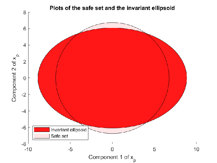
With the secondary controller design, we aim to guarantee that the invariant ellipsoid is a subset of the safe set. If this is feasible, then there exists at least one controller that keeps the closed loop system safe under all attack signals that satisfy the constraint (6).

We choose set $\alpha=0.25$ and $\delta=0.99$ to make the LMI conditions in Corollary 11. We solve these LMIs to obtain

We then choose $M=I_{2}$. The fact that $MN^{\top}=I-XY$ yields $N=\left[\begin{array}[]{cc}-112.9854&0\\ 0&-2.7259\end{array}\right]$. The controller parameters can then be solved as follows in the order of $D_{2}$, $C_{2}$, $B_{2}$, and lastly $A_{2}$ using (27).

It can be seen from Figure 3 that, the found invariant ellipsoid is now a subset of the safe set. Therefore, by adding the secondary controller to the system, we rule out the possibility of unsafe operations of the system subject to attacks satisfying (6). One can also try to minimize $\text{Tr}[X]$ under the constraints given in Corollary 11. Recall that via Lemma 6, we prove that $\text{Tr}[X]$ can be used as a convex upper bound on the volume of $\mathcal{E}_{Q}$, with $Q$ being the projection of $P$ on to the $\zeta_{1}$-hyperplane. The following controller is synthesized if we minimize $\text{Tr}[X]$,

The plot of the invariant ellipsoid is shown in Figure. 4. It can be seen that, the volume of the invariant set in Figure. 4 is significantly reduced compared to the one shown in Figure. 3.

We have used an invariant set based method to provide a framework for checking the safety of LTI systems subject to sensor and actuator attacks by resource limited adversaries. In addition, by using a subset of sensors and secure feedback, a plug-and-play linear secondary controller synthesis problem is also solved to recover the safety of the overall system. The initial synthesis problem is not convex, but can be rendered so with a congruence transformation, which yields an LMI condition that can be solved efficiently. The effectiveness of the proposed design is illustrated via a numerical example, where a secondary controller is designed to guarantee safety which can not be guaranteed by the primary controller alone.

One possible future research direction is the investigation of how to smarly choose the matrices $C_{S}$ and $E_{u}$. In our work, we assume it is given, i.e., the designer first chooses which sensors are to be secured and used for secondary controller design and how the output of the secondary controller is fed back to the plant. When the size of the system is large, it is desired to have a more efficient and intelligent approach to choosing which set of sensors are to be used for the secondary controller.

References

- Ames et al. (2017) Ames, A.D., Xu, X., Grizzle, J.W., and Tabuada, P. (2017). Control barrier function based quadratic programs for safety critical systems. IEEE Transactions on Automatic Control, 62(8), 3861–3876.
- Bai et al. (2015) Bai, C.Z., Pasqualetti, F., and Gupta, V. (2015). Security in stochastic control systems: Fundamental limitations and performance bounds. In 2015 American Control Conference (ACC), 195–200. IEEE.
- Blanchini (1999) Blanchini, F. (1999). Set invariance in control. Automatica, 35(11), 1747–1767.
- Boyd et al. (1994) Boyd, S., El Ghaoui, L., Feron, E., and Balakrishnan, V. (1994). Linear matrix inequalities in system and control theory. SIAM.
- Cárdenas et al. (2008) Cárdenas, A.A., Amin, S., and Sastry, S. (2008). Research challenges for the security of control systems. HotSec, 5, 15.
- Chong et al. (2015) Chong, M.S., Wakaiki, M., and Hespanha, J.P. (2015). Observability of linear systems under adversarial attacks. In 2015 American Control Conference (ACC), 2439–2444. IEEE.
- Dutta and Langbort (2017) Dutta, A. and Langbort, C. (2017). Stealthy output injection attacks on control systems with bounded variables. International Journal of Control, 90(7), 1389–1402.
- Escudero et al. (2022a) Escudero, C., Massioni, P., Zamaï, E., and Raison, B. (2022a). Analysis, prevention, and feasibility assessment of stealthy ageing attacks on dynamical systems. IET Control Theory & Applications, 16(4), 381–397.
- Escudero et al. (2022b) Escudero, C., Murguia, C., Massioni, P., and Zamaï, E. (2022b). Enforcing safety under actuator injection attacks through input filtering. In 2022 European Control Conference (ECC), 1521–1528.
- Fawzi et al. (2014) Fawzi, H., Tabuada, P., and Diggavi, S. (2014). Secure estimation and control for cyber-physical systems under adversarial attacks. IEEE Transactions on Automatic control, 59(6), 1454–1467.
- Kurzhanski and Vályi (1997) Kurzhanski, A. and Vályi, I. (1997). Ellipsoidal calculus for estimation and control. Springer.
- Milošević et al. (2020) Milošević, J., Sandberg, H., and Johansson, K.H. (2020). Estimating the impact of cyber-attack strategies for stochastic networked control systems. IEEE Transactions on Control of Network Systems, 7(2), 747–757.
- Murguia et al. (2020) Murguia, C., Shames, I., Ruths, J., and Nešić, D. (2020). Security metrics and synthesis of secure control systems. Automatica, 115, 108757.
- Romagnoli et al. (2020) Romagnoli, R., Griffioen, P., Krogh, B.H., and Sinopoli, B. (2020). Software rejuvenation under persistent attacks in constrained environments. IFAC-PapersOnLine, 53(2), 4088–4094.
- Scherer et al. (1997) Scherer, C., Gahinet, P., and Chilali, M. (1997). Multiobjective output-feedback control via lmi optimization. IEEE Transactions on automatic control, 42(7), 896–911.
- Tang et al. (2019) Tang, Z., Kuijper, M., Chong, M.S., Mareels, I., and Leckie, C. (2019). Linear system security—detection and correction of adversarial sensor attacks in the noise-free case. Automatica, 101, 53–59.
- Teixeira et al. (2015a) Teixeira, A., Shames, I., Sandberg, H., and Johansson, K.H. (2015a). A secure control framework for resource-limited adversaries. Automatica, 51, 135–148.
- Teixeira et al. (2015b) Teixeira, A., Sou, K.C., Sandberg, H., and Johansson, K.H. (2015b). Secure control systems: A quantitative risk management approach. IEEE Control Systems Magazine, 35(1), 24–45.