Photometry of the Four Anti-Galactocentric Old Open Clusters: Czernik 30, Berkeley 34, Berkeley 75, and Berkeley 76Scipy (Jones et al. 2001), astrometry.net (Lang et al. 2010), IRAF (Tody 1986; Tody 1993), DAOPHOT II/ALLSTAR (Stetson 1990), PARSEC (Bressan et al. 2012), pyUPMASK (Pera et al. 2021).

Most stars in the Milky Way Galaxy (MWG) are born in star clusters (Lada & Lada 2003; Kim et al. 2009; Kyeong et al. 2011). The stars in open clusters (OCs) share some physical values, such as distance, age, and chemical composition, which can be determined using photometric methods (Park & Lee 1999; Kyeong et al. 2001; Kyeong et al. 2008; Ahumada et al. 2013; Carrera et al. 2017). OCs can be divided into three groups by age: old OCs have ages older than 1 Gyr, young OCs have ages younger than 1 Myr, and intermediate-age OCs have ages of 1 Myr $-$ 1 Gyr (Friel 1995). Young OCs are useful for investigating star formation processes, while old OCs are a good tool for research on the formation and early evolution of the Galactic disk and examination of stellar evolution models (van den Bergh & McClure 1980; Lada & Lada 2003).

There are many Galactic OC catalogs. Lyngå  published ‘Catalog of Open Cluster Data’ that includes 1148 OCs with physical parameters, like diameter, age, metallicity, and reddening (Lyngå 1995). Dias et al. 2002 catalog of version 3.5 includes 2167 MWG OCs with the information about location, kinematics, distance, age, and reddening. The Milky Way Star Cluster catalog of Kharchenko et al. 2013 increased the number of OCs to 2808.

The number of OCs in catalogs goes up, but the number of OCs with known physical parameters are much less than the total number of OCs in the catalogs. Since the beginning of the $Gaia$ era, many studies have estimated parameters such as distance and age with $Gaia$. Using the $Gaia$ DR2 data, Cantat-Gaudin et al. 2018a published a list of 1229 OCs including physical parameters like age, distance, proper motion, and parallax. Liu & Pang 2019 included 2443 cluster candidates with parameters from isochrone fitting. Using $Gaia$ DR2 data, the Gaussian mixture model, mean-shift algorithms and visual inspections, Sim et al. 2019 discovered 207 new OCs. Although OC catalogs are being updated, there are disagreements about the physical parameters of the same object among the studies in the catalogs. Cantat-Gaudin et al. 2020 used machine learning method to fit isochrone models to the $Gaia$ DR2 data and obtained parameters (age, distance, and extinction) for 2000 OCs. Dias et al. 2021 provided physical parameters, such as proper motion, radial velocity, distance, age, and [Fe/H], for 1743 OCs based on the $Gaia$ DR2 data.

The old OCs with larger Galactocentric distances are important for studying metallicity distribution in the Galactic disk. Janes 1979 found the Galactic disk metallicity gradient using OCs. Twarog et al. 1997 argued the existence of a discontinuity in radial metallicity distribution outside of 10 kpc from the Galactic center, where the inner part shows a steeper gradient than the outer part. The position of the discontinuity is suggested to be at $10-15$ kpc in recent studies (Netopil et al. 2016; Kim et al. 2017; Donor et al. 2020; Monteiro et al. 2021). However, the number of well-studied OCs at the outer part of the Galactic disk is currently too small to clearly determine the existence and position of the discontinuity.

One of the strengths of studying the anti-Galactocentric region is the relatively lower extinction, which enables us to investigate the evolution of the outer part of the Galactic disk. The old OCs in the anti-Galactocentric region can be a useful tool for studying the evolution of the MWG since they hold a long dynamic timescales (Gaia Collaboration et al. 2021).

We investigated the physical parameters of four OCs located in the anti-Galactocentric direction: Czernik 30, Berkeley 34, Berkeley 75 and Berkeley 76 by using the red clump (RC) stars and by fitting the PAdova and TRieste Stellar Evolution Code (PARSEC) isochrones (Bressan et al. 2012).

In Table 1, we summarize the physical parameters of the four OCs obtained by the previous studies and in our study. Czernik 30 is located at $\alpha_{J2000}=07^{h}31^{m}10.8^{s}$ and $\delta_{J2000}=-09\arcdeg 56\arcmin 42\arcsec$ and has been studied in four literatures. Hasegawa et al. 2008 and Piatti et al. 2009 presented physical parameters using $BVI$ photometric data and Washington photometric data. Perren et al. 2015 made a code for the automatic determination of physical parameters of OCs, and included Czernik 30 in their sample for testing the code and gave the physical parameters. Hayes et al. 2015 conducted a photometric and spectroscopic study of Czernik 30 and obtained the basic parameters.

The position of Berkeley 34 is $\alpha_{J2000}=07^{h}00^{m}23.2^{s}$, $\delta_{J2000}=-00\arcdeg 13\arcmin 54\arcsec$ and there are three previous studies for this cluster. Hasegawa et al. 2004 and Ortolani et al. 2005 presented the physical parameters using isochrone fitting. Donati et al. 2012 presented ranges for the physical parameters and calculated the binary fraction, which is measured from color and magnitude and fine-tuning with differential reddening value.

Berkeley 75 is located at $\alpha_{J2000}=06^{h}48^{m}59.1^{s}$, $\delta_{J2000}=-23\arcdeg 59\arcmin 36\arcsec$. Carraro et al. 2005 published the physical parameters using the $BVI$ photometry and Carraro et al. 2007 studied five OCs at the outer Galactic disk including Berkeley 75 using VLT high resolution spectroscopic data, and suggested the physical parameters. Cantat-Gaudin et al. 2016 studied the abundances and kinematics of ten OCs including Berkeley 75. They used the spectroscopic data of two member stars of Berkeley 75 and gave the [Fe/H] value of Berkeley 75.

The location of Berkeley 76 is $\alpha_{J2000}=07^{h}06^{m}42.4^{s}$, $\delta_{J2000}=-11\arcdeg 43\arcmin 33\arcsec$ and the properties of Berkeley 76 from three previous studies have a relatively wider range. Hasegawa et al. 2008 and Tadross 2008 obtained the physical parameters from isochrone fittings to the $BVI$ photometric data and 2MASS $JHK$ data. Carraro et al. 2013 studied five old OCs at the outer Galactic disk including Berkeley 76 and they determined the parameters. The distance modulus from Hasegawa et al. 2008 and Carraro et al. 2013 differ by almost 3 magnitudes.

This study uses the observation data obtained from the same observing run as that of Kim et al. 2017, which presented the physical parameters of the old OC Ruprecht 6. To better constrain the evolution of the outer part of the Galactic disk, in this paper, we estimate the physical parameters of the four OCs in a way basically consistent with that of Kim et al. 2017 but more improved. In this study, we use the $Gaia$ Early Data Release 3 (EDR3) data to select member stars of the clusters and adopt the number density distribution function of the stellar photometry results, to better estimate the centers and radius of the clusters.

This paper is organized as follows. In Section 2, we explain the observations and data reduction. In Section 3, we describe the results on Czernik 30. Section 3 has five subsections : the center of Czernik 30, radius, member selection using the $Gaia$ EDR3 data, reddening and distance, age and metallicity, and comparison with previous studies. In Sections 4, 5, and 6, we show the results for Berkeley 34, Berkeley 75, and Berkeley 76, respectively, using the same routines as in section 3. In Section 7, we show and discuss the radial metallicity distribution of the Galactic disk, using the previously known OCs from the literature and the newly estimated physical quantities of the four OCs together. In Section 8, we summarize our results.

The $BVI$ images for the four target OCs, Czernik 30, Berkeley 34, Berkeley 75, and Berkeley 76, were acquired at the Small and Moderate Aperture Research Telescope System (SMARTS) 1.0 m telescope with the Y4KCam camera at the Cerro Tololo Inter-American Observatory (CTIO) in 2010 December. Y4KCam has 4064 $\times$ 4064 pixels and the pixel scale is $0.289\arcsec$ pixel^-1 and the field of view (FoV) is $19.57\arcmin\times 19.57\arcmin$. While the R.A. and declination are in Table 1, Table 2 lists Galactic longitudes, Galactic latitudes, and the radii of the four OCs. Figure 1 shows the centers and radii of the OCs together with the center positions from previous studies. Table 3 lists the observation log showing the observation date, filter and exposure times.

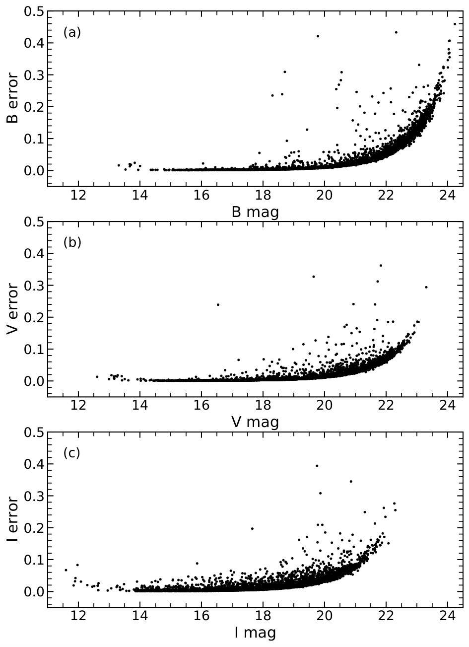
While the reduction and photometry routines were the same as those applied as in Kim et al. 2017, we summarize the key processes here. IRAF¹¹ 1 IRAF is distributed by the National Optical Astronomy Observatories, which is operated by the Association of Universities for Research in Astronomy, Inc. (AURA) under a cooperative agreement with the National Science Foundation./CCDRED package has been used for the standard reduction processes of overscan correction, bias correction, and sky flattening. Point spread function (PSF) photometry has been performed by using the DAOPHOT II/ALLSTAR stand-alone package (Stetson 1990). The error values of the PSF photometry are shown in Fig. 2. To derive the astrometry solution, astrometry.net (Lang et al. 2010) has been used.

Four Landolt standard star fields (PG0231+051, LB1735, LSS982, Rubin 149) (Landolt 1992; Landolt & Uomoto 2007; Landolt 2009) were observed to obtain the standardization equations to convert the instrumental magnitudes to standard magnitudes. The same transformation equations as those in Kim et al. 2017 are used, which are

In the same way as in Czernik 30, we determined the center of Berkeley 34: $\alpha_{J2000}=07^{h}00^{m}23.2^{s}$ and $\delta_{J2000}=-00\arcdeg 13\arcmin 54\arcsec$ (red cross symbol in Fig. 1 (b)) using gaussian_kde package and the distribution function shown in Fig. 6. The center of Berkeley 34 from the previous study is shown in Fig. 1 (b). The green x symbol is $\alpha_{J2000}=07^{h}00^{m}23^{s}$, $\delta_{J2000}=-00\arcdeg 14\arcmin 15\arcsec$ (Ortolani et al. 2005) and the yellow x symbol is $\alpha_{J2000}=07^{h}00^{m}24^{s}$, $\delta_{J2000}=-00\arcdeg 15\arcmin 00\arcsec$ (Hasegawa et al. 2004). Donati et al. 2012 presents $\alpha_{J2000}=07^{h}00^{m}23^{s}$, $\delta_{J2000}=-00\arcdeg 13\arcmin 56\arcsec$ as the center of Berkeley 34, and the magenta x symbol indicates this location.

To select the member stars of Berkeley 34, we adopted the pyUPMASK package (see Section 3.2) using the $Gaia$ proper motion and parallax data. Finally, 147 stars were selected as the members of Berkeley 34 and are shown in Fig. 6 as white-magenta dot symbols.

Fig. 7 shows the radial density profile of Berkeley 34. We determine the radius of Berkeley 34 to be about $2.5\arcmin\pm 0.3\arcmin$ where the member fraction is greater than 0.5 in spite of the existence of members from $2.5\arcmin$ to $4\arcmin$. While Hasegawa et al. 2004 did not specify the radius value adopted in their study, Ortolani et al. 2005 used $r\sim 58\arcsec$ in fitting the isochrones, and Donati et al. 2012 used the stars inside $r\sim 2.5\arcmin$ region.

Fig. 8 shows $V$ vs. $B-V$ and $V$ vs. $V-I$ CMDs for the stars in $r\sim 2.5\arcmin$. The MSTO is located at $V\sim 19.00$ mag, $B-V\sim 0.98$, and $V-I\sim 1.25$. Hasegawa et al. 2004 estimated the MSTO location to be ($V,V-I$) = (18.5, 1.2). Donati et al. 2012 claimed two points for the MS of Berkeley 34: MS red hook (the reddest part of MS) at $V\sim 18.5$ mag and the MS termination point at $V\sim 18.0$ mag.

We took the four stars near $V\sim 16.72$, $B-V\sim 1.58$, and $V-I\sim 1.73$ as the RC stars of Berkeley 34, and thier photometry data are shown in Table 4. From the RC method, we calculate the reddening values $E(J-K_{s})=0.27\pm 0.12$, $E(B-V)=0.56\pm 0.24$, and the distance modulus $(m-M)_{0}=14.13\pm 0.19$ ($d=6.70\pm 0.59$ kpc). Since $\delta V$ index is 2.28, $E(B-V)$ was estimated to be $0.63\pm 0.10$, which is consistent with the value from the RC method. Donati et al. 2012 suggested two groups of RC, brighter and fainter: the position of the brighter RC group was at $V\sim 15.7$ and $B-V\sim 1.7$ and the fainter RC group was located at $V\sim 16.7$ and $B-V\sim 1.55$. We consider only one RC group exists for Berkeley 34, which corresponds to the fainter group in Donati et al. 2012.

We tried to fit the PARSEC isochrones to the CMDs of Berkeley 34 using the reddening and distance modulus derived using the RC method. Fig. 8 shows the best fit PARSEC isochrones with CMDs. Finally, we determined the fundamental physical parameters for Berkeley 34, which include age, metallicity, distance modulus, and color excess: age $\log t=9.40\pm 0.05$ ($t=2.51\pm 0.30$ Gyr), metallicity [Fe/H] $=-0.30\pm 0.15$ dex, distance modulus $(m-M)_{0}=14.13\pm 0.19$ ($d=6.70\pm 0.59$ kpc), and color excesses $E(B-V)=0.56\pm 0.24$ and $E(V-I)=0.73\pm 0.31$.

As shown in Table 1, Hasegawa et al. 2004 obtained age $t=2.8$ Gyr, metallicity $Z=0.019$ ([Fe/H]$=-0.02$), distance $(m-M)_{0}=14.31$, and color excesses $E(B-V)=0.45$ and $E(V-I)=0.60$. Ortolani et al. 2005 obtained the distance to Berkeley 34 of d = $7.8\pm 0.8$ kpc. Donati et al. 2012 measured the physical parameters using Full Spectrum of Turbulence (FST), Padova, Frascati Raphson Newton Evolutionary Code (FRANEC) isochrone. They gave a physical parameters range from the FST isochrone: age from 2.1 to 2.5 Gyr, metallicity $Z=0.01$ ([Fe/H]$=-0.31$ dex), distance from 6 to 7 kpc ($(m-M)_{0}\sim 14.1-14.3$), color excess E($B-V)\sim 0.57-0.64$. Overall, our results show good agreement with the values in the three studies listed above.

In the same way as in Czernik 30, we determined the center of Berkeley 75 using the kernel density estimation method (Fig. 9). Berkeley 75 is located at $\alpha_{J2000}=06^{h}48^{m}59.1^{s}$, $\delta_{J2000}=-23\arcdeg 59\arcmin 36\arcsec$. The green x symbol in Fig. 1 (c) for $\alpha_{J2000}=06^{h}48^{m}59^{s}$ and $\delta_{J2000}=-23\arcdeg 59\arcmin 30\arcsec$ indicates the center position of Berkeley 75 used by Carraro et al. 2005.

By adopting the pyUPMASK package (see Section 3.2), 77 stars were determined to be the members of Berkeley 75. The radial density profile of Berkeley 75 is shown in Fig. 10. The region from $1.9\arcmin$ to $4^{\prime}$ has member stars of Berkeley 75 but field stars represent the majority in this region. Thus, we determined the radius of Berkeley 75 to be $1.9\arcmin$. Carraro et al. 2005 determined the radius of Berkeley 75 to be $1\arcmin$ from its radial density profile.

The CMDs of Berkeley 75 are shown in Fig. 11, where MSTO is located at $V\sim 18.1$ mag, $B-V\sim 0.46$, and $V-I\sim 0.63$. Carraro et al. 2005 also presented almost the same value ($V\approx 18$ mag) for the MSTO.

We selected two RC stars of Berkeley 75, which are listed in Table 4 (c). The mean magnitude and color for the RC stars in Berkeley 75 are $V=15.44\pm 0.11$, $B-V=1.00\pm 0.18$, and $V-I=1.10\pm 0.15$ while Carraro et al. 2005 measured the location of the RCs to be $V\sim 16.0$ mag which is quite different from ours. Using the RC method, we calculated the distance $(m-M)_{0}=14.44\pm 0.17$ ($d=7.73\pm 0.61$ kpc) and reddening $E(B-V)=0.07\pm 0.18$. Using $\delta V$ index of 2.66 and the method of Janes & Phelps 1994, we obtained $E(B-V)=0.05\pm 0.20$, which is consistent with the value from the RC method within error range.

We tried to determine the age and metallicity of Berkeley 75 using the PARSEC isochrones and the reddening and distance values obtained from the RC method, as shown in Fig. 11. We measured age $\log t=9.50\pm 0.10$ ($t=3.16\pm 0.73$ Gyr), metallicity [Fe/H] $=-0.57\pm 0.20$ dex, distance modulus $(m-M)_{0}=14.44\pm 0.17$, and color excesses $E(B-V)=0.07\pm 0.18$ and $E(V-I)=0.13\pm 0.32$. Although the reddening value measured by Janes & Phelps 1994 was not exactly consistent with the reddening value from the RC method, the reddening values were consistent with the values from the RC method within the error range. Carraro et al. 2005 obtained distance modulus $(m-M)=15.2$, color excesses $E(B-V)=0.08$ and $E(V-I)=0.13$ using the Padova isochrones of age 3 Gyr and metallicity $Z=0.004$ ([Fe/H] $=-0.72$ dex). Carraro et al. 2007 revised the estimates to be: age $4.0\pm 0.4$ Gyr, metallicity [Fe/H] $=-0.22\pm 0.20$ dex, distance modulus $(m-M)=14.90\pm 0.20$, and color excess $E(B-V)=0.04\pm 0.03$. The revised parameters of Carraro et al. 2007 show good agreement with our parameters.

Using the kernel density estimation method as in the previous sections, we determined the center of Berkeley 76 as shown in Fig. 12. Unlike the three OCs in the previous sections, Berkeley76 has many more number of stars spread in the field. We determined the center of Berkeley 76 to be at $\alpha_{J2000}=07^{h}06^{m}42.4^{s}$ and $\delta_{J2000}=-11\arcdeg 43\arcmin 33\arcsec$. Carraro et al. 2013 suggested the center of Berkeley 76 to be $\alpha_{J2000}=07^{h}06^{m}24^{s}$ and $\delta_{J2000}=-11\arcdeg 37\arcmin 00\arcsec$. However, since their Fig. 1 and our Fig. 1 (d) show the same region, their center coordinates in their Table 1 might not be correct. The yellow x symbol in our Fig. 1 (d) indicates $\alpha_{J2000}=07^{h}06^{m}44^{s}$ and $\delta_{J2000}=-11\arcdeg 44\arcmin$ from Hasegawa et al. 2008 and the magenta x symbol is $\alpha_{J2000}=07^{h}06^{m}24^{s}$ and $\delta_{J2000}=-11\arcdeg 37\arcmin 38\arcsec$ from Tadross 2008. The center location from Tadross 2008 is quite far away ($7.51\arcmin$) from the center in our study.

288 stars are selected as members of Berkeley 76 from the pyUPMASK algorithm (Pera et al. 2021) with $Gaia$ EDR3 proper motion and parallax data. In Fig. 13, the trend in the radial density profile of Berkeley 76 is different from those in the three OCs of the previous sections. $4.0\arcmin\pm 0.3\arcmin$ is determined to be the radius of Berkeley 76 where the member fraction is 0.5. Carraro et al. 2013 used $2\arcmin$ as the radius of Berkeley 76 and Tadross 2008 obtained $4.5\arcmin$ for the radius of Berkeley 76.

Fig. 14 shows the $V$ vs. $B-V$ and $V$ vs. $V-I$ CMDs for Berkeley 76, where the five RC stars can be seen at $V\sim 16.22\pm 0.08$, $B-V\sim 1.35\pm 0.06$, and $V-I\sim 1.59\pm 0.03$. The photometry results for these five stars are shown in Tab. 4 (d). We determined the distance and reddening of Berkeley 76 using the RC method: distance modulus $(m-M)_{0}=13.97\pm 0.23$ and reddening $E(B-V)=0.41\pm 0.33$. $\delta V$ index of Berkeley 76 is 2.04, and this gives us $E(B-V)=0.39\pm 0.12$ which is consistent with that from the RC method.

Carraro et al. 2013 suggested the mean magnitude and color for the four RC stars in Berkeley 76 to be $V\sim 17.9$ and $B-V\sim 1.4$, respectively. While the $B-V$ colors are in very good agreement with their color and ours, their $V$ magnitude is $\sim 1.7$ mag fainter than ours. Considering two things, that (1) the two CMDs in our study (Fig. 14) and Carraro et al. 2013 (their Fig. 7) are very similar, and (2) the distance modulus estimated by Carraro et al. 2013 ($(m-M)_{0}=17.20\pm 0.15$) is much larger than those of Hasegawa et al. 2008 ($(m-M)_{0}=14.39$) and our study ($(m-M)_{0}=13.97\pm 0.23$), we suspect the $V$ magnitudes in Carraro et al. 2013 were somehow shifted by $\sim+1.7$ mag.

We tried to find best fit PARSEC isochrones using the distance and the reddening values from the RC method as shown in Fig. 14. We determined the physical parameters: age $\log t=9.10\pm 0.05$ ($t=1.26\pm 0.14$ Gyr), metallicity [Fe/H] $=0.00\pm 0.20$ dex, distance modulus $(m-M)_{0}=13.97\pm 0.23$ ($d=6.22\pm 0.66$ kpc), and color excesses $E(B-V)=0.41\pm 0.33$ and $E(V-I)=0.57\pm 0.46$.

OCs can help reveal the chemical evolution of the Galactic disk (Netopil et al. 2016; Kim et al. 2017; Chen & Zhao 2020; Donor et al. 2020; Spina et al. 2021; Zhang et al. 2021; Netopil et al. 2022). Netopil et al. 2016 mentioned the importance of a homogeneous data set and they obtained the Galactic metaillicity distribution from a homogeneous data set of 172 OCs for three ranges, which is divided at $R_{GC}\sim 9$ and $12$ kpc. Donor et al. 2020 studied the chemical abundance distribution of the Galactic disk using OC data from the Sloan Digital Sky Survey/APOGEE DR 16, and they determined the [Fe/H] vs $R_{GC}$ has a slope of $-0.068\pm 0.001$ dex kpc^-1 in the region of $6<R_{GC}<13.9$ kpc from the Markov Chain Monte Carlo method. Spina et al. 2021 found the slope of [Fe/H] over $R_{GC}$ to be $-0.076\pm 0.009$ dex kpc^-1 using a bayesian regression with the spectroscopic data of 134 OCs from GALactic Archaeology with HERMES (GALAH) survey or APOGEE survey. Spina et al. 2022 gathered high-resolution spectroscopic surveys data and measured $-0.064\pm 0.007$ dex kpc^-1 as the metallicity gradient. They also suggested a flat metallicity distribution at outside of $R_{GC}=12.1\pm 1.1$ kpc.

We combined the distances and the [Fe/H] values from the following five catalogs, together with the data for the four OCs obtained in this study : Dias et al. 2002, Netopil et al. 2016, Donor et al. 2020, Spina et al. 2021, and Dias et al. 2021. Dias et al. 2002; Dias et al. 2021 are the OC catalogs including the physical parameters such as age, distance and metallicity. Netopil et al. 2016, Donor et al. 2020, and Spina et al. 2021 focused on the chemical evolution in the Galactic disk. If there were more than two [Fe/H] values, we tried to use the values from the spectroscopic data, if they exist, expecting them to have higher accuracy. We used 8 kpc as the solar distance from the Galactic center, $R_{GC,\odot}$. The number of old OCs in the final catalog is 236.

Fig. 15 shows the Galactic radial metallicity distribution of the OCs with ages older or younger than 1 Gyr. We tried applying a single linear fit (panel (a)) and a broken linear fit (panel (b)) to the combined data for OCs with $t\geq 1$ Gyr. The broken linear fit assumes the existence of discontinuity and uses two linear functions for the fit, with the final result listed in Table 5. While the existence of the discontinuity is a controversial issue, several possibilities are suggested as causes of the metallicity distribution in the Galactic disk: for example, radial migration (Minchev et al. 2013; Minchev et al. 2018; Zhang et al. 2021; Netopil et al. 2022), metal enrichment (Monteiro et al. 2021), etc.

The number of OCs younger than 1 Gyr shown in Fig. 15 (c) is negligible in the outer part of the Galactic disk, especially outside of 14.5 kpc. The small number of samples at the outer part in Fig. 15 (b) make the broken linear fit look more suitable than the single linear fit. For the broken linear fit in Fig. 15 (b), we tried to find the appropriate location of the discontinuity from 12 kpc to 14 kpc using a step size of 0.5 kpc. The discontinuity at 12 kpc has, naturally, the largest number of old OCs at the outer region, hence, the Bayesian information criteria (BIC)²² 2 the BIC statistic is a method for scoring and selecting a model, and the model with the lowest BIC is selected. value at 12 kpc was the smallest among those from 12 kpc to 14 kpc. When using the old OCs as elements to investigate the metallicity distribution in the Galactic disk, it is important to increase the number of samples at the outer region, especially outside of 14 kpc, for better analysis. Although the addition of the four old OCs from our study to Fig. 15 is not a significant increase in the number of the sample, our data are relatively important in that all the four clusters are located at the outer region of $r\sim 14$ kpc.

In this paper, we investigated four old OCs in the MWG. We photometrically determined their physical quantities and compared them with those in previous studies. By combining data of the four OCs with those from previously known OCs, we newly estimated the radial metallicity distribution of the MWG. We summarize our results as follows (see also Table 1 and Table 2).

• •

  We determined the center of Czernik 30 - $\alpha_{J2000}=07^{h}31^{m}10.8^{s}$, $\delta_{J2000}=-09\arcdeg 56\arcmin 42\arcsec$. We estimated the physical parameters: radius $2.3^{\prime}\pm 0.3^{\prime}$, color excess $E(B-V)=0.15\pm 0.08$, age $t=2.82\pm 0.32$ Gyr ($\log t=9.45\pm 0.05$), metallicity [Fe/H]$=-0.22\pm 0.15$ dex, and distance modulus $(m-M)_{0}=14.05\pm 0.13$.

• •

  We determined the center of Berkeley 34 - $\alpha_{J2000}=07^{h}00^{m}23.2^{s}$, $\delta_{J2000}=-00\arcdeg 13\arcmin 54\arcsec$. We estimated the quantities: radius $2.5^{\prime}\pm 0.3^{\prime}$, color excess $E(B-V)=0.56\pm 0.24$, age $t=2.51\pm 0.30$ Gyr$(\log t=9.40\pm 0.05)$, metallicity [Fe/H] $=-0.30\pm 0.15$ dex, and distance modulus $(m-M)_{0}=14.13\pm 0.19$.

• •

  We determined the center of Berkeley 75 - $\alpha_{J2000}=06^{h}48^{m}59.1^{s}$, $\delta_{J2000}=-23\arcdeg 59\arcmin 36\arcsec$. As for the physical quantities : radius $1.9^{\prime}\pm 0.2^{\prime}$, color excess $E(B-V)=0.07\pm 0.18$, age $t=3.16\pm 0.73$ Gyr ($\log t=9.50\pm 0.10$), metallicity [Fe/H] $=-0.57\pm 0.20$ dex, and distance modulus $(m-M)_{0}=14.44\pm 0.17$.

• •

  We determined the center of Berkeley 76 - $\alpha_{J2000}=07^{h}06^{m}42.4^{s}$ and $\delta_{J2000}=-11\arcdeg 43\arcmin 33\arcsec$. For the physical quantities: we obtained radius $4.0^{\prime}\pm 0,3^{\prime}$, color excess $E(B-V)=0.41\pm 0.33$, age $t=1.26\pm 0.14$ Gyr ($\log t=9.10\pm 0.05$), metallicity [Fe/H] $=0.00\pm 0.20$ dex, and distance modulus $(m-M)_{0}=13.97\pm 0.23$.

• •

  We investigated the radial metallicity distribution of the Galactic disk using a single linear fit and a broken linear fit to 236 old OCs. The gradient of the single linear fit was $-0.052\pm 0.004$ dex kpc^-1, and those for the broken linear fit were $-0.070\pm 0.006$ dex kpc^-1 at $r<12$ kpc and $-0.016\pm 0.010$ at $r\geq 12$ kpc.

References

- Ahumada et al. (2013) Ahumada, A. V., Cignoni, M., Bragaglia, A., et al. 2013, MNRAS, 430, 221, doi: 10.1093/mnras/sts593
- Alves (2000) Alves, D. R. 2000, ApJ, 539, 732, doi: 10.1086/309278
- Bessell (2001) Bessell, M. S. 2001, PASP, 113, 66, doi: 10.1086/317972
- Bressan et al. (2012) Bressan, A., Marigo, P., Girardi, L., et al. 2012, MNRAS, 427, 127, doi: 10.1111/j.1365-2966.2012.21948.x
- Cannon (1970) Cannon, R. D. 1970, MNRAS, 150, 111, doi: 10.1093/mnras/150.1.111
- Cantat-Gaudin et al. (2016) Cantat-Gaudin, T., Donati, P., Vallenari, A., et al. 2016, A&A, 588, A120, doi: 10.1051/0004-6361/201628115
- Cantat-Gaudin et al. (2018a) Cantat-Gaudin, T., Jordi, C., Vallenari, A., et al. 2018a, A&A, 618, A93, doi: 10.1051/0004-6361/201833476
- Cantat-Gaudin et al. (2018b) Cantat-Gaudin, T., Vallenari, A., Sordo, R., et al. 2018b, A&A, 615, A49, doi: 10.1051/0004-6361/201731251
- Cantat-Gaudin et al. (2020) Cantat-Gaudin, T., Anders, F., Castro-Ginard, A., et al. 2020, A&A, 640, A1, doi: 10.1051/0004-6361/202038192
- Carraro et al. (2013) Carraro, G., Beletsky, Y., & Marconi, G. 2013, MNRAS, 428, 502, doi: 10.1093/mnras/sts038
- Carraro et al. (2005) Carraro, G., Geisler, D., Moitinho, A., Baume, G., & Vázquez, R. A. 2005, A&A, 442, 917, doi: 10.1051/0004-6361:20053089
- Carraro et al. (2007) Carraro, G., Geisler, D., Villanova, S., Frinchaboy, P. M., & Majewski, S. R. 2007, A&A, 476, 217, doi: 10.1051/0004-6361:20078113
- Carrera et al. (2017) Carrera, R., Rodríguez Espinosa, L., Casamiquela, L., et al. 2017, MNRAS, 470, 4285, doi: 10.1093/mnras/stx1526
- Carrera et al. (2019) Carrera, R., Pasquato, M., Vallenari, A., et al. 2019, A&A, 627, A119, doi: 10.1051/0004-6361/201935599
- Chan & Bovy (2020) Chan, V. C., & Bovy, J. 2020, MNRAS, 493, 4367, doi: 10.1093/mnras/staa571
- Chen et al. (2017) Chen, Y. Q., Casagrande, L., Zhao, G., et al. 2017, ApJ, 840, 77, doi: 10.3847/1538-4357/aa6d0f
- Chen & Zhao (2020) Chen, Y. Q., & Zhao, G. 2020, MNRAS, 495, 2673, doi: 10.1093/mnras/staa1079
- Dias et al. (2002) Dias, W. S., Alessi, B. S., Moitinho, A., & Lépine, J. R. D. 2002, A&A, 389, 871, doi: 10.1051/0004-6361:20020668
- Dias et al. (2021) Dias, W. S., Monteiro, H., Moitinho, A., et al. 2021, MNRAS, 504, 356, doi: 10.1093/mnras/stab770
- Donati et al. (2012) Donati, P., Bragaglia, A., Cignoni, M., Cocozza, G., & Tosi, M. 2012, MNRAS, 424, 1132, doi: 10.1111/j.1365-2966.2012.21289.x
- Donor et al. (2020) Donor, J., Frinchaboy, P. M., Cunha, K., et al. 2020, AJ, 159, 199, doi: 10.3847/1538-3881/ab77bc
- Francis & Anderson (2014) Francis, C., & Anderson, E. 2014, MNRAS, 441, 1105, doi: 10.1093/mnras/stu631
- Friel (1995) Friel, E. D. 1995, ARA&A, 33, 381, doi: 10.1146/annurev.aa.33.090195.002121
- Gaia Collaboration et al. (2021) Gaia Collaboration, Antoja, T., McMillan, P. J., et al. 2021, A&A, 649, A8, doi: 10.1051/0004-6361/202039714
- Girardi (2016) Girardi, L. 2016, ARA&A, 54, 95, doi: 10.1146/annurev-astro-081915-023354
- Grocholski & Sarajedini (2002) Grocholski, A. J., & Sarajedini, A. 2002, AJ, 123, 1603, doi: 10.1086/339027
- Groenewegen (2008) Groenewegen, M. A. T. 2008, A&A, 488, 935, doi: 10.1051/0004-6361:200810201
- Hasegawa et al. (2004) Hasegawa, T., Malasan, H. L., Kawakita, H., et al. 2004, PASJ, 56, 295, doi: 10.1093/pasj/56.2.295
- Hasegawa et al. (2008) Hasegawa, T., Sakamoto, T., & Malasan, H. L. 2008, PASJ, 60, 1267, doi: 10.1093/pasj/60.6.1267
- Hawkins et al. (2017) Hawkins, K., Leistedt, B., Bovy, J., & Hogg, D. W. 2017, MNRAS, 471, 722, doi: 10.1093/mnras/stx1655
- Hayes et al. (2015) Hayes, C. R., Friel, E. D., Slack, T. J., & Boberg, O. M. 2015, AJ, 150, 200, doi: 10.1088/0004-6256/150/6/200
- Janes (1979) Janes, K. A. 1979, ApJS, 39, 135, doi: 10.1086/190568
- Janes & Phelps (1994) Janes, K. A., & Phelps, R. L. 1994, AJ, 108, 1773, doi: 10.1086/117192
- Jones et al. (2001) Jones, E., Oliphant, T., & Peterson, P. 2001, SciPy: Open Source Scientific Tools for Python. http://www.scipy.org
- Kharchenko et al. (2013) Kharchenko, N. V., Piskunov, A. E., Schilbach, E., Röser, S., & Scholz, R. D. 2013, A&A, 558, A53, doi: 10.1051/0004-6361/201322302
- Kim (2006) Kim, S. C. 2006, Journal of Korean Astronomical Society, 39, 115, doi: 10.5303/JKAS.2006.39.4.115
- Kim et al. (2017) Kim, S. C., Kyeong, J., Park, H. S., et al. 2017, Journal of Korean Astronomical Society, 50, 79, doi: 10.5303/JKAS.2017.50.3.79
- Kim et al. (2009) Kim, S. C., Kyeong, J., & Sung, E.-C. 2009, Journal of Korean Astronomical Society, 42, 135, doi: 10.5303/JKAS.2009.42.6.135
- Kim & Sung (2003) Kim, S. C., & Sung, H. 2003, Journal of Korean Astronomical Society, 36, 13, doi: 10.5303/JKAS.2003.36.1.013
- Krone-Martins & Moitinho (2014) Krone-Martins, A., & Moitinho, A. 2014, A&A, 561, A57, doi: 10.1051/0004-6361/201321143
- Kyeong et al. (2008) Kyeong, J., Kim, S. C., Hiriart, D., & Sung, E.-C. 2008, Journal of Korean Astronomical Society, 41, 147, doi: 10.5303/JKAS.2008.41.6.147
- Kyeong et al. (2011) Kyeong, J., Moon, H.-K., Kim, S. C., & Sung, E.-C. 2011, Journal of Korean Astronomical Society, 44, 33, doi: 10.5303/JKAS.2011.44.1.033
- Kyeong et al. (2001) Kyeong, J.-M., Byun, Y.-I., & Sung, E.-C. 2001, Journal of Korean Astronomical Society, 34, 143, doi: 10.5303/JKAS.2001.34.3.143
- Lada & Lada (2003) Lada, C. J., & Lada, E. A. 2003, ARA&A, 41, 57, doi: 10.1146/annurev.astro.41.011802.094844
- Landolt (1992) Landolt, A. U. 1992, AJ, 104, 340, doi: 10.1086/116242
- Landolt (2009) —. 2009, AJ, 137, 4186, doi: 10.1088/0004-6256/137/5/4186
- Landolt & Uomoto (2007) Landolt, A. U., & Uomoto, A. K. 2007, AJ, 133, 768, doi: 10.1086/510485
- Laney et al. (2012) Laney, C. D., Joner, M. D., & Pietrzyński, G. 2012, MNRAS, 419, 1637, doi: 10.1111/j.1365-2966.2011.19826.x
- Lang et al. (2010) Lang, D., Hogg, D. W., Mierle, K., Blanton, M., & Roweis, S. 2010, AJ, 139, 1782, doi: 10.1088/0004-6256/139/5/1782
- Liu & Pang (2019) Liu, L., & Pang, X. 2019, ApJS, 245, 32, doi: 10.3847/1538-4365/ab530a
- Lyngå (1995) Lyngå, G. 1995, VizieR Online Data Catalog, VII/92A
- Minchev et al. (2013) Minchev, I., Chiappini, C., & Martig, M. 2013, A&A, 558, A9, doi: 10.1051/0004-6361/201220189
- Minchev et al. (2018) Minchev, I., Anders, F., Recio-Blanco, A., et al. 2018, MNRAS, 481, 1645, doi: 10.1093/mnras/sty2033
- Monteiro et al. (2021) Monteiro, H., Barros, D. A., Dias, W. S., & Lépine, J. R. D. 2021, Frontiers in Astronomy and Space Sciences, 8, 62, doi: 10.3389/fspas.2021.656474
- Netopil et al. (2022) Netopil, M., Oralhan, İ. A., Çakmak, H., Michel, R., & Karataş, Y. 2022, MNRAS, 509, 421, doi: 10.1093/mnras/stab2961
- Netopil et al. (2016) Netopil, M., Paunzen, E., Heiter, U., & Soubiran, C. 2016, A&A, 585, A150, doi: 10.1051/0004-6361/201526370
- Nishiyama et al. (2009) Nishiyama, S., Tamura, M., Hatano, H., et al. 2009, ApJ, 696, 1407, doi: 10.1088/0004-637X/696/2/1407
- Ortolani et al. (2005) Ortolani, S., Bica, E., Barbuy, B., & Zoccali, M. 2005, A&A, 439, 1135, doi: 10.1051/0004-6361:20041458e
- Park & Lee (1999) Park, H. S., & Lee, M. G. 1999, MNRAS, 304, 883, doi: 10.1046/j.1365-8711.1999.02366.x
- Pera et al. (2021) Pera, M. S., Perren, G. I., Moitinho, A., Navone, H. D., & Vazquez, R. A. 2021, A&A, 650, A109, doi: 10.1051/0004-6361/202040252
- Perren et al. (2015) Perren, G. I., Vázquez, R. A., & Piatti, A. E. 2015, A&A, 576, A6, doi: 10.1051/0004-6361/201424946
- Phelps et al. (1994) Phelps, R. L., Janes, K. A., & Montgomery, K. A. 1994, AJ, 107, 1079, doi: 10.1086/116920
- Piatti et al. (2009) Piatti, A. E., Clariá, J. J., Parisi, M. C., & Ahumada, A. V. 2009, New A, 14, 97, doi: 10.1016/j.newast.2008.05.006
- Ruiz-Dern et al. (2018) Ruiz-Dern, L., Babusiaux, C., Arenou, F., Turon, C., & Lallement, R. 2018, A&A, 609, A116, doi: 10.1051/0004-6361/201731572
- Sim et al. (2019) Sim, G., Lee, S. H., Ann, H. B., & Kim, S. 2019, Journal of Korean Astronomical Society, 52, 145, doi: 10.5303/JKAS.2019.52.5.145
- Skrutskie et al. (2006) Skrutskie, M. F., Cutri, R. M., Stiening, R., et al. 2006, AJ, 131, 1163, doi: 10.1086/498708
- Spina et al. (2022) Spina, L., Magrini, L., & Cunha, K. 2022, Universe, 8, 87, doi: 10.3390/universe8020087
- Spina et al. (2021) Spina, L., Ting, Y. S., De Silva, G. M., et al. 2021, MNRAS, 503, 3279, doi: 10.1093/mnras/stab471
- Stetson (1990) Stetson, P. B. 1990, PASP, 102, 932, doi: 10.1086/132719
- Tadross (2008) Tadross, A. L. 2008, MNRAS, 389, 285, doi: 10.1111/j.1365-2966.2008.13554.x
- Tody (1986) Tody, D. 1986, in Society of Photo-Optical Instrumentation Engineers (SPIE) Conference Series, Vol. 627, Instrumentation in astronomy VI, ed. D. L. Crawford, 733, doi: 10.1117/12.968154
- Tody (1993) Tody, D. 1993, in Astronomical Society of the Pacific Conference Series, Vol. 52, Astronomical Data Analysis Software and Systems II, ed. R. J. Hanisch, R. J. V. Brissenden, & J. Barnes, 173
- Twarog et al. (1997) Twarog, B. A., Ashman, K. M., & Anthony-Twarog, B. J. 1997, AJ, 114, 2556, doi: 10.1086/118667
- van den Bergh & McClure (1980) van den Bergh, S., & McClure, R. D. 1980, A&A, 88, 360
- van Helshoecht & Groenewegen (2007) van Helshoecht, V., & Groenewegen, M. A. T. 2007, A&A, 463, 559, doi: 10.1051/0004-6361:20052721
- Wang & Chen (2021) Wang, S., & Chen, X. 2021, ApJ, in print, arXiv:2108.13605. https://arxiv.org/abs/2108.13605
- Zhang et al. (2021) Zhang, H., Chen, Y., & Zhao, G. 2021, ApJ, 919, 52, doi: 10.3847/1538-4357/ac0e92
- Zhong et al. (2022) Zhong, J., Chen, L., Jiang, Y., Qin, S., & Hou, J. 2022, AJ, 164, 54, doi: 10.3847/1538-3881/ac77fa