Joint Estimation of Clustered User Activity and Correlated Channels with Unknown Covariance in mMTC

Sparse signal recovery techniques have widely been applied in the design of massive machine-type communications (mMTC) solutions with grant-free access protocols. A major challenge in grant-free access is the joint user identification and channel estimation (JUICE). Subsequently, owing to the sporadic nature of activity pattern of the mMTC devices, namely user equipments (UEs), the JUICE has been widely addressed as a sparse recovery problem and solved using various algorithms such as approximate message passing (AMP), sparse Bayesian learning (SBL), and mixed-norm minimization.

The vast majority of the works address the JUICE in an uncorrelated channel model [1, 2, 3, 4, 5, 6]. However, this assumption is not practical as the multiple-input multiple-output (MIMO) channels are usually spatially correlated [7]. Recently, few works have addressed the JUICE in the correlated MIMO channels, thereby better reflecting the reality, using AMP in [8, 9] and using mixed-norm minimization in [10, 11, 12]. Nonetheless, these works assume that channel distribution information (CDI) for all the UEs is available at the base station (BS), which can be challenging to acquire in realistic environments. Furthermore, the prior work on the JUICE considers mMTC networks with a random UE activity pattern. This could model, e.g., a scenario where UEs monitor independent random processes and thus activate randomly based on certain application criteria.

This paper makes the following two distinctions from the prior works: First, we address the JUICE in spatially correlated MIMO channels with no prior knowledge of the exact CDI. Second, we consider an mMTC network where the UEs activity has a specific structure, namely, a clustered form. For instance, this models a network where the UEs form clusters based on their geographical locations and each cluster is associated with a monitoring task. Here, an event could trigger a small subset of UEs belonging to a cluster to activate concurrently, leading to clustered UE activity system-wise.

This paper adopts a Bayesian approach and formulates the JUICE as a maximum a posteriori probability (MAP) estimation problem that takes into consideration the different specific structures of the system model. In particular, to accommodate the clustered activity of the UEs, we propose a log-sum based prior function composed of two different components to capture both the overall sparsity and the clustered sparsity of the signal model. Furthermore, in order to estimate the CDI as well, we utilize a prior function that follows a Wishart distribution. Subsequently, we derive a computationally-efficient iterative solution based on alternating direction method of multipliers (ADMM) that solves an approximate version of the MAP problem as a sequence of closed-form updates.

We consider a single-cell uplink network consisting of $N$ UEs served by a single BS equipped with a uniform linear array (ULA) of $M$ antennas. The UEs are geographically distributed so that they form $C$ clusters, where each cluster contains $L$ UEs¹¹ 1 For the simplicity of presentation, yet without loss of generality, we assume that all clusters contain the same number of UEs., such that ${N=LC}$. A cluster containing a subset of UE indices is denoted by $\mathcal{C}_{l}\subseteq\{1,2,\ldots,N\}$.

The propagation channel between the $i$th UE and the BS, denoted by ${\bf{h}}_{i}$, follows a local scattering model [13]. Thus, each ${\bf{h}}_{i}$ is modelled as a zero-mean complex Gaussian random variable, i.e., ${{\bf{h}}_{i}\sim\mathcal{CN}(0,{\boldsymbol{\Sigma}}_{i}^{-1})}$, where ${\boldsymbol{\Sigma}}_{i}\in\mathbb{C}^{M\times M}$ denotes the channel precision matrix, i.e., the inverse covariance matrix ${{\boldsymbol{\Sigma}}_{i}^{-1}=\mathbb{E}[{\bf{h}}_{i}{\bf{h}}_{i}^{\mbox{\scriptsize H}}]}$. We consider UEs with low mobility, which is justified in mMTC, e.g., in applications like industrial monitoring. Hence, we adopt the common assumption that the channels are wide-sense stationary. Thus, the set of channel precision matrices ${{\boldsymbol{\Sigma}}=\{{\boldsymbol{\Sigma}}_{i}\}_{i=1}^{N}}$ vary in a slower timescale compared to the channel realizations [7].

Since the UE activation is sporadic in mMTC, only a small number of the $N$ UEs are active at each coherence time $T_{\mathrm{c}}$. To this end, the UE activity indicator vector ${{\boldsymbol{\gamma}}=[\gamma_{1},\ldots,\gamma_{N}]^{\mbox{\scriptsize T}}}$ is given as

Contrary to the majority of the literature on mMTC that consider random UE activation, we consider that the UEs activate in a specific clustered manner. More precisely, the active UEs belong to a small (random) number of active clusters, where an active cluster refers to any cluster with at least one active UE, while containing at most ${L_{\mathrm{c}}\leq L}$ active UEs. Such cluster sparsity imposes a special structure on ${\boldsymbol{\gamma}}=[\underbrace{\gamma_{1},\ldots,\gamma_{L}}_{\footnotesize\mbox{Cluster~1}},\underbrace{\gamma_{L+1},\ldots,\gamma_{2L}}_{\footnotesize\mbox{Cluster~2}},\ldots,\underbrace{{\boldsymbol{\gamma}}_{N-L+1},\ldots,{\boldsymbol{\gamma}}_{N}}_{\footnotesize\mbox{Cluster~}C}]$ where the elements belonging to a given cluster ($\gamma_{i}$, $i\in\mathcal{C}_{l}$) are assumed to be correlated. The correlation in the UE activity is imposed by the priors presented in Section 3.3.

For data transmission, each UE $i\in\mathcal{N}$ is assigned a unique unit-norm pilot sequence ${\boldsymbol{\phi}}_{i}\in\mathbb{C}^{\tau_{\mathrm{p}}}$, as well as a transmit power $p_{i}$ that is inversely proportional to its average channel gain [4, 14]. Accordingly, the received pilot signal ${\bf{Y}}\in\mathbb{C}^{\tau_{\mathrm{p}}\times M}$ is given by

where ${{\bf{X}}=[{\bf{x}}_{1},\ldots,{\bf{x}}_{N}]\in\mathbb{C}^{M\times N}}$ denotes the effective channel matrix with ${{\bf{x}}_{i}=\gamma_{i}\sqrt{p_{i}}{\bf{h}}_{i}}$, ${\bf{\Phi}}=[{\boldsymbol{\phi}}_{1},\ldots,{\boldsymbol{\phi}}_{N}]\in\mathbb{C}^{\tau_{\mathrm{p}}\times N}$ is the pilot book, and ${\bf{W}}\sim\mathcal{CN}(0,\,\sigma^{2}{\bf{I}}_{M})\in\mathbb{C}^{\tau_{\mathrm{p}}\times M}$ represents additive white Gaussian noise.

The signal model in (2) represents a linear measurement where the (unknown) effective channel matrix ${\bf{X}}^{\mbox{\scriptsize T}}$ exhibits row sparsity. Thus, detecting the active UEs and estimating their channel gives rise to a sparse recovery problem from a multiple measurement vector (MMV) setup, which can be solved via several CS algorithms. For instance, the Bayesian AMP algorithm [15] can be utilized if the statistics of a sparse signal are known a priori. However, when such information is not available, mixed-norm minimization [16] using deterministic sparsity regularization is often utilized. Clearly, the additional prior information in AMP leads to superior performance in general. However, attaining prior CDI is a nontrivial task and requires network resources to perform a training phase.

In this paper, we aim to tackle the aforementioned issue related to the acquisition of CDI by adopting a Bayesian framework which aims at not only detecting the active UEs and estimate their channels, but also estimating their covariance matrices. More precisely, by formulating the JUICE as an MAP estimation problem and using the adequate prior functions, we develop a computationally-efficient algorithm that solves a relaxed version of the MAP problem iteratively via a set of closed-form update rules, as we show next.

The MAP estimates $\{\hat{{\bf{X}}},\hat{\gamma},\hat{{\boldsymbol{\Sigma}}}\}$ with respect to the posterior density given the measurement matrix ${\bf{Y}}$ is given by

where $(a)$ follows from the Markov chain ${\{{\boldsymbol{\gamma}},{\bf{{\boldsymbol{\Sigma}}}}\}\rightarrow{\bf{X}}\rightarrow{\bf{Y}}}$ and because $p({\bf{Y}})$ does not affect the maximization and $(b)$ follows from the additive Gaussian noise model in (2) and independence of UE activity and channels. Next, we elaborate the definition of the conditional PDF $p({\bf{X}}|{\boldsymbol{\gamma}})$ and the choice of the priors $p({\boldsymbol{\Sigma}})$ and $p({\boldsymbol{\gamma}})$.

For deriving the proposed solution, we make two technical choices:

1) Inspired by the argument raised in [18], aiming to estimate all $N$ precision matrices ${\boldsymbol{\Sigma}}_{i}$ with the available data at the BS may lead to overfitting. Thus, we restrict the estimation of the $N$ precision matrices ${\boldsymbol{\Sigma}}_{i}$ to $L$ precision matrices ${\boldsymbol{\Sigma}}_{l}$. More precisely, we assume that all propagation channels of the UEs within a single cluster share the same CDI, i.e., ${\bf{h}}_{i}\sim\mathcal{CN}({\bf{0}},{\boldsymbol{\Sigma}}_{l}^{-1})$, ${\forall i\in\mathcal{C}_{l}}$, ${\forall l=1,\ldots,C}$.

2) The binary nature of ${\boldsymbol{\gamma}}$ renders the MAP estimation problem intractable for large $N$. To overcome this challenge, we note that finding the index set $\{i\mid\gamma_{i}\neq 0,\;i\in\mathcal{N}\}$ is equivalent to finding the index set $\{i\mid\|{\bf{x}}_{i}\|>0,\;i\in\mathcal{N}\}$. Thus, we can eliminate the variable ${\boldsymbol{\gamma}}$ from the optimization problem by approximating each $\gamma_{i}$ by $\|{\bf{x}}_{i}\|$ and by relaxing $p({\boldsymbol{\gamma}})$ by an equivalent prior function $p({\bf{X}})$ that depends on $\|{\bf{x}}_{i}\|$, $\forall i\in\mathcal{N}$, as we will show in the next section.

By using the aforementioned arguments and substituting (5) and (7) into (3), the MAP estimation problem can be rewritten as

where regularization weights $\beta_{1}$, $\beta_{2}$, and $\beta_{3}$ control the emphasis on the priors with respect to the measurement fidelity term.

In the following, we propose an iterative solution by alternating $p({\bf{X}})$ over $J_{\mathrm{c}}(\cdot)$ and $J_{\mathrm{s}}(\cdot)$. The central idea is to develop an iterative two-level algorithm, whose outer loop aims at detecting the active clusters, and the inner loop aims at detecting the active UEs in each of the estimated active cluster. More precisely, in the outer loop, the algorithm enforces the detection of active clusters via the cluster-sparsity-promoting prior $J_{\mathrm{c}}$ in (9). Subsequently, the algorithm runs an inner loop over the just-estimated active clusters to detect the individual active UEs belonging to them by using the sparsity-promoting prior $J_{\mathrm{s}}$ in (8). The algorithm details are presented next.

Consider a network with one BS equipped with ${M=20}$ antennas serving a ${N=500}$ UEs distributed equally over ${C=20}$ clusters, where ${K=16}$ UEs are active at each $T_{\mathrm{c}}$. Each UE is assigned a unique unit-norm pilot sequence that is generated from an i.i.d. complex Bernoulli distribution. We set each ${\bf{B}}_{l},\forall l$, as ${\bf{B}}_{l}=\zeta{\boldsymbol{\Psi}}_{l}+(1-\zeta)\frac{1}{L}\sum_{i\in\mathcal{C}_{l}}{\boldsymbol{\Sigma}}_{i}$, where ${\boldsymbol{\Psi}}_{l}$ is a random semi-definite Hermitian matrix to model the error in the prior knowledge on the true precision matrix ${\boldsymbol{\Sigma}}_{l}$, whereas the parameter $\zeta$ controls the level of average mismatch between ${\boldsymbol{\Sigma}}_{i}$ and ${\bf{B}}_{l}$, $\forall i\in\mathcal{C}_{l}$, and it is set as $\zeta=0.1$.

Channel estimation is quantified in terms of normalized mean square error (NMSE) defined as $\frac{\mathbb{E}\left[\|{\bf{X}}-\hat{{\bf{X}}}_{\mathcal{S}}\|_{\mathrm{F}}^{2}\right]}{\mathbb{E}\left[\|{\bf{X}}\|_{\mathrm{F}}^{2}\right]},$ where the expectation is computed via Monte-Carlo averaging over all sources of randomness. UEs activity detection is quantified in terms of support recovery rate (SRR), defined as $\frac{|\mathcal{S}\cap\hat{\mathcal{S}}|}{|\mathcal{S}-\hat{\mathcal{S}}|+K}$, where $\hat{\mathcal{S}}$ denotes the detected support by a given algorithm.

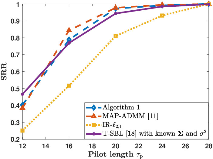
The performance of proposed Algorithm 1 is compared with: 1) iterative reweighted $\ell_{2,1}$ (IR-$\ell_{2,1}$) via ADMM [10], 2) MAP-ADMM [11], and 3) T-SBL [18], where for MAP-ADMM and T-SBL, both ${\boldsymbol{\Sigma}}$ and $\sigma^{2}$ are known to the BS. For an optimal NMSE benchmark, we consider the oracle minimum mean square error (MMSE) estimator having prior knowledge on the true set of active UEs and their covariance matrices.

We consider two cases for UEs’ activity pattern: 1) clustered: with 2 active clusters, each with $8$ active UEs, and 2) random, where ${K=16}$ active UEs are randomly distributed among the clusters.

Fig. 1(a) presents the SRR against the pilot length for the clustered activity pattern. The result shows that Algorithm 1 provides the highest SSR, which can be explained by the fact that Algorithm 1 effectively exploits the clustered structure of the activity pattern using the proposed prior functions. Similarly, the proposed algorithm moderately outperforms MAP-ADMM and T-SBL in terms of NMSE (Fig. 1(b)). In summary, Fig. 1 clearly shows the utility of the proposed algorithm in JUICE with clustered activity patterns.

Fig. 2(a) illustrates the SRR for the random activation scenario. Algorithm 1 achieves performance similar to MAP-ADMM and T-SBL while providing significant gains over IR-$\ell_{2,1}$. On the other hand, Fig. 2(b) shows that while the proposed algorithm clearly outperforms IR-$\ell_{2,1}$ in terms of channel estimation accuracy, it provides just a slightly inferior NMSE performance compared to T-SBL and MAP-ADMM. These results show the robustness of the proposed algorithm to the structure of the activity pattern: the pattern can deviate from the desired clustered form to fully random activity, rendering the algorithm effective for a wide range of UE activity models.

We derived a Bayesian framework to address the JUICE with clustered activity in mMTC under correlated MIMO channels without prior knowledge of the exact CDI. To encourage solutions with cluster sparsity, we proposed a cluster-sparsity-promoting function that correlates the activity of the UEs belonging to the same cluster. We developed an ADMM algorithm that provides a computationally-efficient solution via a sequence of closed-form update rules. The numerical results showed the improvement and robustness brought by the proposed algorithm.

References

- [1] Zhilin Chen, Foad Sohrabi, and Wei Yu, “Sparse activity detection for massive connectivity,” IEEE Trans. Signal Processing, vol. 66, no. 7, pp. 1890–1904, 2018.
- [2] Liang Liu and Wei Yu, “Massive connectivity with massive MIMO—part I: Device activity detection and channel estimation,” IEEE Trans. Signal Processing, vol. 66, no. 11, pp. 2933–2946, 2018.
- [3] Liang Liu and Wei Yu, “Massive connectivity with massive MIMO—part II: Achievable rate characterization,” IEEE Trans. Signal Processing, vol. 66, no. 11, pp. 2947–2959, 2018.
- [4] Kamil Senel and Erik G Larsson, “Grant-free massive MTC-enabled massive MIMO: A compressive sensing approach,” IEEE Trans. Commun., vol. 66, no. 12, pp. 6164–6175, 2018.
- [5] Malong Ke, Zhen Gao, Yongpeng Wu, Xiqi Gao, and Robert Schober, “Compressive sensing-based adaptive active user detection and channel estimation: Massive access meets massive MIMO,” IEEE Trans. Signal Processing, vol. 68, pp. 764–779, 2020.
- [6] Xiaoxu Zhang, Ying-Chang Liang, and Jun Fang, “Novel Bayesian inference algorithms for multiuser detection in M2M communications,” IEEE Trans. Veh. Technol., vol. 66, no. 9, pp. 7833–7848, 2017.
- [7] Luca Sanguinetti, Emil Björnson, and Jakob Hoydis, “Towards massive MIMO 2.0: Understanding spatial correlation, interference suppression, and pilot contamination,” IEEE Trans. Commun., vol. 68, no. 1, pp. 232–257, 2020.
- [8] Yiyao Cheng, Lei Liu, and Li Ping, “Orthogonal AMP for massive access in channels with spatial and temporal correlations,” IEEE J. Select. Areas Commun., vol. 39, no. 3, pp. 726–740, 2021.
- [9] Jianan Bai and Erik G. Larsson, “Activity detection in distributed mimo: Distributed amp via likelihood ratio fusion,” IEEE Wireless Commun. Lett, pp. 1–1, 2022.
- [10] Hamza Djelouat, Markus Leinonen, and Markku Juntti, “Iterative reweighted algorithms for joint user identification and channel estimation in spatially correlated massive mtc,” in ICASSP 2021 - 2021 IEEE International Conference on Acoustics, Speech and Signal Processing (ICASSP), 2021, pp. 4805–4809.
- [11] Hamza Djelouat, Markus Leinonen, and Markku Juntti, “Spatial correlation aware compressed sensing for user activity detection and channel estimation in massive MTC,” IEEE Trans. Wireless Commun., vol. 21, no. 8, pp. 6402–6416, 2022.
- [12] H. Djelouat, M. Leinonen, L. Ribeiro, and M. Juntti, “Joint user identification and channel estimation via exploiting spatial channel covariance in mMTC,” IEEE Wireless Commun. Lett, vol. 10, no. 4, pp. 887–891, 2021.
- [13] Emil Björnson, Jakob Hoydis, and Luca Sanguinetti, “Massive MIMO networks: Spectral, energy, and hardware efficiency,” Foundations and Trends® in Signal Processing, vol. 11, no. 3-4, pp. 154–655, 2017.
- [14] Emil Björnson, Luca Sanguinetti, and Merouane Debbah, “Massive MIMO with imperfect channel covariance information,” in Proc. Annual Asilomar Conf. Signals, Syst., Comp., 2016, pp. 974–978.
- [15] Jongmin Kim, Woohyuk Chang, Bangchul Jung, Dror Baron, and Jong Chul Ye, “Belief propagation for joint sparse recovery,” arXiv preprint arXiv:1102.3289, 2011.
- [16] Christian Steffens, Marius Pesavento, and Marc E Pfetsch, “A compact formulation for the mixed-norm minimization problem,” IEEE Trans. Signal Processing, vol. 66, no. 6, pp. 1483–1497, 2018.
- [17] Christopher M Bishop and Nasser M Nasrabadi, Pattern recognition and machine learning, vol. 4, 2006.
- [18] Zhilin Zhang and Bhaskar D. Rao, “Sparse signal recovery with temporally correlated source vectors using sparse Bayesian learning,” IEEE J. Select. Topics Signal Processing, vol. 5, no. 5, pp. 912–926, 2011.
- [19] Stephen Boyd, Neal Parikh, Eric Chu, Borja Peleato, Jonathan Eckstein, et al., “Distributed optimization and statistical learning via the alternating direction method of multipliers,” Foundations and Trends® in Machine learning, vol. 3, no. 1, pp. 1–122, 2011.