Anyon condensation and the color code

We develop the theory of anyon condensation for Abelian anyon models in the earlier sections of this work, and we investigate various instances of anyon condensation with the color code, and its applications to fault-tolerant quantum computing, in the following sections of the manuscript. We have therefore written the latter sections of the paper in a self-contained way, assuming the reader is familiar with the theory we present in the former sections. We summarise this structure in Table 1, where the different examples of anyon condensation in the latter sections of the paper are presented in the rows of the table, with respect to the different types of anyon condensation that are represented by the columns of the table. Furthermore, we offer the following guide for the reader to navigate through the various sections of the manuscript, where we emphasise the dependence of the latter sections on requisite material from former sections.

In Sec. II, we review the requisite background for the color-code model, and we identify its keys properties that enable it to give rise to a number of non-trivial condensation operations. We then give a general theory for anyon condensation in Sec. III. Specifically, we distinguish between maximal, partial, and trivial condensation. These different types of anyon condensation are distinguished by how excitations are transmitted across the domain wall that is produced by the condensation operation. Again, we show the different types of condensation are represented by the columns of Table 1.

Assuming the reader is familiar with the material presented in Sec. II and Sec. III, the microscopic examples of condensation in the following sections can be read independently. Indeed, Secs. IV and V are self contained. Sec. IV investigates domain walls that spatially separate the color code from one of its condensates, either the vacuum phase, the toric code, or the color code itself. This is represented by the first row of Table 1. Then, in Sec. V, we investigate the different types of condensation over time-like domain walls, as shown in the second row of Table 1.

Sec. VI builds on the ideas we begin to develop in Secs. IV and V. In this section we describe new topological features that are produced by interfacing two phases with an intermediate condensate. Specifically, at the microscopic level, we show that we can make non-trivial domain walls between the color code and itself to produce different types of twist defects, where the color code phase is interfaced by a non-trvial condensate. This construction is represented on the third row of Table 1.

Finally, we discuss our Floquet code construction from the perspective of anyon condensation in Section VII. This picture we present for Floquet codes in terms of condensation operations is represented by the fourth and final row of Table 1. This section can also be read independently of Secs. IV, V and VI.

Anyons are quasi-particles that exist in two spatial dimensions Kitaev 2003; Kitaev 2006. We denote the set of all anyons of a phase, and the data describing their behaviour, by the anyon model $\mathcal{C}$. We label single anyons as lower case letters ${\texttt{a}},{\texttt{b}},{\texttt{c}}\in\mathcal{C}$. The trivial anyon, or the vacuum, which is part of every anyon model, is denoted as 1. Let us now discuss how fusion, exchange and braiding of anyons is described.

Fusion is the process of bringing two anyons close together such that they behave as a third anyon within the same anyon model. We denote fusion by the $\times$ operation. Here, we concentrate on Abelian anyon models where fusion outcomes are unique. The fusion rules of Abelian anyon models are of the form ${\texttt{a}}\times{\texttt{b}}={\texttt{c}}$ for ${\texttt{a}},{\texttt{b}},{\texttt{c}}\in\mathcal{C}$. Fusion with the vacuum anyon is trivial, ${\texttt{a}}\times{\texttt{1}}={\texttt{a}}$. Furthermore, each anyon has an anti-particle with which it fuses to the vacuum. In the topological phases of interest here, namely the color code and toric code, all anyons are their own anti-particles, such that ${\texttt{a}}\times{\texttt{a}}={\texttt{1}}$.

Exchanging two identical Abelian anyons results in a complex phase. If we exchange the position of a pair of a anyons, we denote the obtained phase as $\theta_{\texttt{a}}$. This phase is called spin and for qubit stabiliser codes takes values $\pm 1$. Anyons for which the self-exchange results in a $+1$ ($-1$) phase are called bosons (fermions).

Braiding is the process of moving one anyon around another before returning it to its initial position. Let us say we braid anyon a around a second stationary anyon b, this process results in a phase called monodromy, denoted as $M_{{\texttt{a}},{\texttt{b}}}$. For the color code and toric code phases, the monodromy can only take values $M_{{\texttt{a}},{\texttt{b}}}=\pm 1$, allowing us to use a short-hand formulation calling braiding either trivial ($M_{{\texttt{a}},{\texttt{b}}}=+1$) or non-trivial ($M_{{\texttt{a}},{\texttt{b}}}=-1$).

In fact, it is worth pointing out that the self consistency conditions governing Abelian anyon models lead to a number of redundancies in the data. The identity $M_{{\texttt{a}},{\texttt{b}}}=\theta_{\texttt{a}}\theta_{\texttt{b}}/\theta_{{\texttt{a}}\times{\texttt{b}}}$, for example, lets us determine the self-exchange statistics of any anyon by decomposing it into two different anyons whose spin and relative braid statistics are known.

We can define a microscopic, local Hamiltonian, composed of commuting Pauli interaction terms acting on qubits such that the ground space is the common $+1$ eigenspace of all the terms that give rise to a topological phase. We say that violated interaction terms occupy quasi-particle excitations. These excitations may behave like anyons. Unitary rotations create and transport anyons, allowing us to study their fusion, self-exchange and braiding explicitly Bombín 2014. In the next two sections, we study two specific examples of Hamiltonian models, the color code and the toric code.

In what follows, we introduce a lattice model realising the color code Bombín and Martin-Delgado 2006 before turning our attention to the anyonic excitation it hosts. We employ the language of stabiliser codes Gottesman 1997 to describe the microscopic lattice models realising topologically ordered phases. Stabiliser codes are defined by an Abelian subgroup of the Pauli group that we call the stabiliser group. Importantly, the common $+1$ eigenspace of the elements of the stabiliser group specifies the code space of a code. The group therefore does not include $-1$ as this operator has only negative eigenvalues. We measure stabiliser operators to detect errors.

The color code can be defined on any lattice which is three-colourable with respect to its faces. We use the colours red, green and blue. It is also helpful to assign colors to the edges of the lattice. The colour of an edge is given by the colour of the faces it connects. In this work, we focus on the hexagonal lattice, as shown in Fig. 1.

To specify the color code we assign physical qubits to the vertices of the three-colourable lattice, and stabilisers are associated to the plaquettes of the lattice. We index the plaquettes with the symbol $p$. Each plaquette hosts two stabiliser generators, one of which acts in the $X$-basis on all qubits supported on the plaquette, $s_{X}^{p}$, the other in the $Z$-basis, denoted $s_{Z}^{p}$. We will refer to them as $X$-type or $Z$-type stabilisers respectively. Note, by multiplying the two stabiliser generators on any plaquette, we obtain a $Y$-type stabiliser at plaquette $p$, i.e., $s_{Y}^{p}=s_{Z}^{p}s_{X}^{p}$.

Given the stabilisers of a code, we can introduce a commuting Hamiltonian consisting of the negative sum of a set of stabiliser generators. For topological stabiliser codes, these Hamiltonian terms commute and can be chosen to be geometrically local. In the color code, we usually pick the plaquette terms $s_{X}^{p}$ and $s_{Z}^{p}$ acting in the Pauli-$X$ and Pauli-$Z$ basis on all qubits surrounding a plaquette $p$, as depicted in Fig. 1. This yields the following Hamiltonian,

The ground state space of this Hamiltonian coincides with the code-space of the stabiliser code. Excited eigenstates are reached when some plaquette terms are violated. These states differ from states in the ground state space by Pauli-rotations on single qubits. We associate the violated plaquette terms with anyonic excitations and say they are created by said Pauli rotations.

Let us now discuss color code anyons and their properties. The color code phase contains 16 anyons. Apart from the vacuum excitation, there are 9 non-trivial bosons. Each boson has one of three color labels, r, g, b, as well as one of three Pauli labels, x, y, z. The labels are given by the colour of the violated plaquette and the basis of the Pauli rotation which create and move the anyons. As an example, we say that a red plaquette whose stabiliser(s) are violated by an applied Pauli-$X$ rotation is associated with an anyon labelled rx. See Fig. 1 (a), for example.

Throughout this work, we find it instructive to order the $9$ color-code bosons in a $3\times 3$-table Kesselring et al. 2018, such that bosons in any given row (column) share their Pauli- (colour-) label. This table is referred to as the color-code boson table

Let us review how the data of the color-code anyons are captured by the boson table (2). All color-code anyons are their own anti particles, hence two identical anyons fuse to the trivial anyon. For example we get ${\texttt{rx}}\times{\texttt{rx}}={\texttt{1}}$. Bosons which lie in the same row or column, fuse to the third boson in said row or column. Examples of such fusions are ${\texttt{bx}}\times{\texttt{by}}={\texttt{bz}}$ or ${\texttt{gy}}\times{\texttt{by}}={\texttt{ry}}$. Braiding between two bosons from the same row or column is trivial, e.g., $M_{{\texttt{rx}},{\texttt{ry}}}=M_{{\texttt{gz}},{\texttt{bz}}}=+1$, whereas bosons from differing rows and columns braid non-trivially, e.g., $M_{{\texttt{gx}},{\texttt{rz}}}=-1$.

Fusing two bosons which differ in both Pauli- and colour-label, results in one of six fermions

Writing color-code fermions in terms of their composite bosons lets us infer all of their relevant data. For example, using rules we have defined in the previous section, (Sec. II.1) we find that fermions labelled with an even number label braid trivially with fermions labelled by an odd number, e.g., $M_{{\texttt{f${}_{1}$}},{\texttt{f${}_{4}$}}}=+1$, whereas two distinct even (odd) fermions braid non-trivially, e.g., $M_{{\texttt{f${}_{3}$}},{\texttt{f${}_{5}$}}}=-1$.

To store quantum information in the color code, we can either place the code on a topologically non-trivial manifold, or we can introduce boundaries. We define the different boundary types of the color code in terms of anyon condensation in subsection IV.1. The prototypical example of an quantum error-correcting code in the color-code phase is the triangular color code, depicted in Fig. 2 (a). We associate a code distance $d$ with the code, given by the weight of its least-weight logical operator. The code depicted in Fig. 2 (a), for example, has a code distance $d=7$. Importantly, we have a family of codes that can be parameterised by their code distance that diverges. Assuming we have access to a sensible decoder Wang et al. 2010; Landahl et al. 2011; Bombin et al. 2012; Sarvepalli and Raussendorf 2012; Delfosse and Nickerson 2017; Aloshious and Sarvepalli 2018; Li 2018; Tuckett et al. 2019; Li et al. 2020; Chubb 2021; Sabo et al. 2021; Sahay and Brown 2022, we can correct all error configurations that affect fewer than some number of qubits that diverges in the code distance $d$. As we discuss in Sec. IV.1, logical operators in the color code appear as strings along non-trivial paths. In codes with boundaries, such paths may connect distinct boundaries or enclose punctures. This means that by increasing the system size, i.e., by separating boundaries further apart or enlarging punctures, we can increase the code distance. This in turn means that we can tolerate more errors. Assuming errors happen sufficiently rarely, we can decrease the probability of a logical error occurring arbitrarily close to zero by increasing the code distance.

In this section, we discuss the well known toric code phase; a topologically ordered phase that is closely related to the color code. The toric code, introduced by Kitaev in Ref. Kitaev 2003, is widely regarded as the prototypical example of a topological stabiliser code. Its associated phase is referred to as the toric code phase, or simply the toric code. Here, we will briefly review its anyonic excitations and introduce an example of a microscopic lattice model in the toric code phase.

There are four anyons in the anyon model of the low-energy theory of the toric code. The particle 1 represents the vacuum, or the trivial anyon. Particles e and m are bosonic anyons with $\theta_{\texttt{e}}=\theta_{\texttt{m}}=+1$, and f is a fermion with $\theta_{\texttt{f}}=-1$. The anyons fuse as follows, ${\texttt{e}}\times{\texttt{e}}={\texttt{m}}\times{\texttt{m}}={\texttt{f}}\times{\texttt{f}}={\texttt{1}}$ and ${\texttt{e}}\times{\texttt{m}}={\texttt{f}}$. Any two non-identical, non-trivial anyons braid non-trivially, e.g., $M_{{\texttt{e}},{\texttt{m}}}=-1$.

Fig. 3 shows a construction for the toric code which is particularly helpful for our discussion throughout this work. We start with a hexagonal lattice, place a physical qubit on each vertex and colour the plaquettes as in Fig. 3. Each plaquette hosts a stabiliser generator acting on the surrounding qubits in a Pauli-basis defined by the colour of the plaquette. Green and blue plaquettes host weight-6 $Z$-type stabilisers. Red plaquettes and red edges host weight-6 and weight-2 $X$-type stabilisers, respectively. The same stabilisers are obtained when following Kitaev’s original toric code construction Kitaev 2003 on a triangular lattice decorated with additional 2-valent vertices on every edge, as shown in Fig. 3. In Kitaev’s original description of the toric-code model, qubits are placed on the edges of some arbitrary lattice. Then, Pauli-X stabilisers are associated to the vertices of the lattice and Pauli-Z stabilisers are associated to the faces of the lattice. Specifically, Pauli-X vertex stabilizers (Pauli-Z plaquette stabilisers) are the product of Pauli-X (Pauli-Z) terms on qubits associated to edges adjacent to their respective lattice vertex (plaquette). See also the matching code construction Wootton 2015 which describes a construction for microscopic stabiliser models in the toric code phase based on Kitaev’s honeycomb model Kitaev 2006, including the model described here. The excitations on red plaquettes and edges are e anyons. The blue and green plaquettes host the m anyon.

The color code is equivalent to two decoupled layers of the toric code Bombin et al. 2012; Kubica et al. 2015; Criger and Terhal 2016, meaning that the anyon model from two decoupled layers of toric codes is equivalent to the anyon model of the color code. One way of mapping the color code anyon labels to the labels given by two layers of toric codes is

where ${\texttt{1}},{\texttt{e}},{\texttt{m}},{\texttt{f}}$ are the toric code anyons and their position in the tuple a b represents on which of the two layers they live. We refer to (9) as the standard unfolding. There are, however, $72$ valid ways to perform the unfolding, which can be obtained by applying one of the $72$ anyon permuting symmetries of the color code Yoshida 2015; Kesselring et al. 2018 to the standard mapping (9). Furthermore, we can identify the six fermions of the color code as follows,

In two-dimensional topological stabiliser codes, we detect errors by measuring stabiliser generators to obtain a list of violated stabilisers Kitaev 2003; Dennis et al. 2002. In reality, however, these stabiliser measurements may be imperfect and give incorrect outcomes. To achieve tolerance to noise in the presence of measurement errors, we must repeat the measurements multiple times Dennis et al. 2002; Wang et al. 2003. This transforms the space in which the stabiliser violations live into a $(2+1)$-dimensional space-time.

As we have described violated stabilisers can be associated with anyonic quasi-particles. This association carries over to the case where we consider the full space-time picture of the stabiliser readouts. In fact, from a condensed matter perspective, this is very natural, as all two-dimensional topologically ordered phases and processes happening therein are described in as a $(2+1)$-dimensional space-time. In what follows, we make this connection explicit.

We begin by replacing the stabiliser generators associated with plaquettes with detection cells Dennis et al. 2002; Wang et al. 2003; Gidney 2021. For simplicity, we assume that all stabiliser readouts are performed in parallel. Each detection cell is associated with one position in space-time $(s,t)$, given by the location of a stabiliser generator $s$ and a time-step $t$. A detection cell compares the outcome of the measurement of stabiliser $s$ during the $t$-th round with the result obtained for $s$ in the $(t-1)$-th round, see Fig. 4 (a). Thus, they detect changes in measurement outcomes which might be caused by errors on the physical qubits they support or when a faulty measurement result is obtained.

Now, we associate anyonic quasi particles with (single or sets of) violated stabiliser cells. A detection cell $(s,t)$ detects errors occurring on physical qubits in the support of $s$ between time steps $t-1$ and $t$, see Fig. 4 (b). This is exactly analogous to the purely two-dimensional viewpoint, like we show it in Fig. 1, where we interpret errors as creating sets of anyons with neutral total charge. Importantly, a detection cell $(s,t)$ also detects measurement errors affecting $s$ in round $t-1$ or in round $t$. Thus, a single measurement error occurring when measuring the stabiliser at $s$ in round $t$ thus violates two detection cells, $(s,t-1)$ and $(s,t)$, see Fig. 4 (b). Such a process can be though of as a pair-creation in the time direction of an anyon associated with the violation of $s$. In general, strings are composed of both, measurement errors as well as errors on physical data qubits, and create point-like anyons in space-time. As an example, we shown a world-line of a color code anyon in Fig. 4 (d).

Thus, a two-dimensional topological error-correcting code where measurements are repeated over time correspond to a microscopic model realised in $(2+1)$-dimensional space-time. This allows us on the one hand to explicitly study topological processes taking place in time using topological stabiliser codes as toy models. And on the other hand, we can draw on the wealth of results obtained in the mathematical study of topologically ordered $(2+1)$-dimensional phases of matter and apply them in real-world error correcting schemes. With this in mind, let us turn our attention to anyon condensation.

At the end of Sec. II.2, we touched on the fault tolerance of the color code. Let us here make this definition more precise while including errors affecting the measurements of stabiliser terms. As we have seen, errors in the $(2+1)$-dimensional space-time can be interpreted as segments of strings with anyons at their end-points. Crucially, due to measurement errors, these error strings can also travel along the temporal direction.

Logical errors occur when sufficiently many errors appear along non-trivial paths, connecting distinct boundaries Dennis et al. 2002; Strikis et al. 2021. Importantly, these can be spatial boundaries (see Sec. IV.1) as well as temporal boundaries (see Sec. V.2). This means that we need to include errors affecting measurement outcomes into our definition of the code distance $d$. The code distance $d$ of a code is the lowest number of errors – including measurement errors – which results in a non-detectable and non-trivial logical error. In this work, we call a protocol fault tolerant, if $d$ grows extensively with the system size. In other words, by increasing the system size in the two spatial and in the temporal direction, we can reach an arbitrarily low logical error rate assuming a suitable decoder and physical error rate below threshold.

Anyon condensation is a mechanism to relate certain anyon models to each other. Given a parent Abelian anyon theory $\mathcal{C}$, a $\mathcal{C}$-condensate $\mathcal{C}_{\mathcal{B}}$ is obtained by identifying a subgroup of bosons $\mathcal{B}\subset\mathcal{C}$ with the trivial charge. An anyon in the condensed theory $\mathcal{C}_{\mathcal{B}}$ is related to a coset of anyons ${\texttt{a}}\mathcal{B}\subset\mathcal{C}$.

In particular, we start by choosing a bosonic subgroup, meaning a subgroup of bosons that is closed under fusion and that contains only bosons with trivial mutual braid statistics. Next, we identify this subgroup $\{{\texttt{b}}_{1},{\texttt{b}}_{2},\ldots\}=\mathcal{B}\subset\mathcal{C}$ with the trivial charge,

Hence, a pair of anyons ${\texttt{a}},{\texttt{b}}\in\mathcal{C}$ that differ by fusion with some elements of $\mathcal{B}$ become identified in the condensate. In the remainder if the paper, we use the notation

Let us look at the different ways anyons of the parent theory can be affected by condensation. The anyons of the parent theory $\mathcal{C}$ fall into two classes.

• •

  Deconfined: Any anyon a that braids trivially with all elements in $\mathcal{B}$, is deconfined

  $\displaystyle{\texttt{a}}\equiv{\texttt{a}}\mathcal{B}\quad\mbox{iff}\quad M_{{\texttt{a}},{\texttt{b}}}=1~\forall~{\texttt{b}}\in\mathcal{B}.$

  (14)

  The anyon a from the parent theory then defines the anyon ${\texttt{a}}\mathcal{B}$ in the condensed theory.

• •

  Confined: If ${\texttt{a}}\in\mathcal{C}$ braids non-trivially with at least one element in $\mathcal{B}$, the topological spin of ${\texttt{a}}\mathcal{B}$ becomes ill-defined and a therefore becomes confined. The object ${\texttt{a}}\mathcal{B}$ is not an anyon in the condensed theory.

Anyons of a condensate $\mathcal{C}_{\mathcal{B}}$, defined by condensing a bosonic subgroup $\mathcal{B}\subset\mathcal{C}$, are in one-to-one correspondence with a subset of cosets $\{{\texttt{a}}\mathcal{B}\,|\,M_{{\texttt{a}},{\texttt{b}}}=1\,\forall~{\texttt{b}}\in\mathcal{B}\}$. The modular data of the condensate is given by the parent theory

The constraint on $\mathcal{B}$ being a set of bosons, all of which braid trivially with a and b, ensures that the topological numbers of a and b are the same. Furthermore, it is apparent that $\mathcal{B}$ must be closed under fusion.

Throughout this work, we will make use of symmetries in a given parent theory to relate different condensates. A symmetry of anyon model $\mathcal{C}$ is a permutation of the anyon labels that leaves the anyonic data invariant. The group formed by all these permutations is called the automorphism group of the anyon model, $\Aut(\mathcal{C})$. In general, a symmetry in the parent maps a bosonic subgroup $\mathcal{B}$ to a (potentially different) bosonic subgroup $\mathcal{B}^{\prime}$. The fact that it is a symmetry of the parent indicates that $\mathcal{C}_{\mathcal{B}}$ is in the same phase as $\mathcal{C}_{\mathcal{B}^{\prime}}$. Symmetries that preserve $\mathcal{B}$ turn into symmetries in the condensate.

In this section, we define different types of anyon condensation. We use the color-code anyon model to exemplify different condensation mechanisms.

A domain wall is a one-dimensional subregion along which two phases interface. The type of interfaces we consider in this work correspond to gapped domain walls between two (Abelian) topologically ordered phases $\mathcal{C}$ and $\mathcal{C}^{\prime}$ Beigi et al. 2011; Kitaev and Kong 2012. Anyon condensation proves to be a useful tool to study this class of domain walls. Furthermore, it is worth pointing out that this description is agnostic towards the space-time direction along which the phases are interfaced. This means that our following prescription will hold for domain walls that cut any plane of the $(2+1)$-dimensional space-time.

We can interface two anyon models $\mathcal{C}$ and $\mathcal{C}^{\prime}$ iff they share a common condensate $\mathcal{C}_{\mathcal{B}}\simeq\mathcal{C}^{\prime}_{\mathcal{B}^{\prime}}$.

The domain wall can then be interpreted as a thin strip of the condensate between the two phases, as shown in Fig. 5. Anyons in $\mathcal{B}$ ($\mathcal{B}^{\prime}$) condense at the domain wall. Anyons that braid non-trivially with any of the condensed anyons get confined to one side of the domain wall, meaning that they cannot move without creating additional excitations. Anyons that braid trivially with all bosons in $\mathcal{B}$ ($\mathcal{B}$’) are deconfined and can move through the domain wall. For this reason, in this context we call them mobile.

We can derive consistency conditions on how the anyonic data on one side of the domain wall relates to the other following Fig. 6.

Let ${\texttt{a}},{\texttt{b}},{\texttt{c}}$ be anyons in $\mathcal{C}$ which, when moved through a domain wall get mapped to ${\texttt{a}}^{\prime},{\texttt{b}}^{\prime},{\texttt{c}}^{\prime}\in\mathcal{C}^{\prime}$. World-lines realising the three processes of fusion, self-exchange and braiding can smoothly be deformed to lie on either side of the domain wall. Hence, they must result in consistent outcomes. This implies that the anyonic data on either side of the domain wall must be the same, i.e., we have that

Furthermore, we can obtain the conditions on anyons which condense at a boundary in this fashion. To this end, we equate $\mathcal{C}^{\prime}$ to the trivial phase, which we can think of as only hosting the trivial anyon. This means all processes happening on this side of the domain wall must be trivial. From this we get closure under fusion and the triviality of self-exchange and braiding of condensible anyons, see Eq. (15).

Domain walls can be classified by the number of bosons they can condense. For the color code this means that the domain walls fall into three classes opaque, semi-transparent and invertible. All types will appear with different applications in Secs. IV, V and VI.

Opaque domain walls are obtained when a full Lagrangian subgroup of bosons can condense from both sides. The corresponding condensate is the trivial phase and they have no mobile anyons.

We call a domain wall semi-transparent if certain anyons remain mobile while others condense at the domain wall. Semi-transparent domain walls within the same phase can be terminated within the bulk.

Invertible domain walls can only be realised within the same phase using trivial condensation. Anyons crossing the domain wall need to preserve their data, hence invertible domain walls are in one-to-one correspondence with the elements of the automorphism group of the anyon model, $\Aut(\mathcal{C})$. The endpoints of invertible domain walls are called twist defects and behave similar to non-Abelian anyons in terms of fusion and braiding Bombín 2010; Brown et al. 2017; Barkeshli et al. 2019; Kesselring et al. 2018; Bridgeman and Barter 2020.

So far, we have discussed anyon condensation on an abstract level in terms of anyons. In what follows, we turn our attention to microscopic realisations of topologically ordered phases using stabiliser models. In particular, we describe how to derive a stabiliser model for a condensate from a stabiliser model of a parent phase $\mathcal{S}_{\mathcal{C}}$. Microscopically, we achieve this by adding hopping terms of the condensed bosons to the stabiliser, effectively modelling the process of anyon condensation. While we only consider qubit stabilisers explicitly here, the procedure can be generalised to stabilisers on qudits Ellison et al. 2022 and even for non-Pauli models Bombín and Martin-Delgado 2008, if one knows the microscopic description of the string operators of the code. Finally, we show how to make the construction explicit by constructing the toric-code stabiliser model (see Sec. II.3) from the color-code stabiliser model (see Sec. II.1).

To bridge from the abstract notion of anyon condensation to microscopic models, let us reframe stabiliser operators of topological codes in terms of anyons and their string operators. Both the color code and toric code, as introduced in Sec. II, are topological lattice models whose code space corresponds to the ground space of a topologically ordered Hamiltonian. In any topological lattice model elementary excitations, anyons, are created at the endpoints of string operators which are supported on one-dimensional subregions, see for example Fig. 1 (a). This means that any closed string operator does not create any excitation and thereby leaves the ground space invariant. In this reading, stabilisers correspond to contractible loops of the aforementioned string operators. Measuring a stabiliser is equivalent to performing an interferometric charge measurement Bombín 2014.

We now make the abstract notion of anyon condensation from Sec. III explicit in microscopic lattice models. In a condensate, we require that string operators that transport condensed bosons $\mathcal{B}$ do not change the state, as we identify them with the trivial charge. We achieve this by adding all open string operators transporting bosons in $\mathcal{B}$ to the stabiliser group. This can be achieved, for instance, by adding the set of shortest hopping terms as generators of the stabiliser group.

These string operators violate some of the original stabiliser terms. To recover a commuting stabiliser group that describes the condensate, the terms of the original stabiliser group that do not commute with the new hopping terms are removed. This step corresponds to removing confined charges from the anyon model of the condensed phase.

In the following, we give a recipe to construct the stabiliser group of a condensate from a parent theory $\mathcal{C}$ and its stabiliser group $\mathcal{S}_{\mathcal{C}}$ and a bosonic subgroup $\mathcal{B}\subset\mathcal{C}$.

1. 1.

   Define the group $\mathcal{S}_{\mathcal{B}}$ of open string operators for $\mathcal{B}$ generated hopping terms.

2. 2.

   Remove the stabilisers from $\mathcal{S}_{\mathcal{C}}$ that do not commute with $\mathcal{S}_{\mathcal{B}}$. These correspond to the closed string operators of the anyons that braid non-trivially with at least one anyon in $\mathcal{B}$. We denote the reduced stabiliser group as $\widetilde{\mathcal{S}}_{\mathcal{C}}$.

3. 3.

   The stabiliser group of the condensed phase $\mathcal{C}_{\mathcal{B}}$ is given by $\widetilde{\mathcal{S}}_{\mathcal{C}}\cup\mathcal{S}_{\mathcal{B}}$.

This construction shows how the toric code is a condensate of the color code. We can view the $XX$ stabilisers on the red links, characteristic for the microscopic realisation of the toric code introduced in Sec. II.3, as the hopping terms of the rx anyon in the color code. Following the procedure laid out above, where $\mathcal{S}_{\mathcal{C}}$ is the color code and $\mathcal{S}_{\mathcal{B}}$ is generated by the $XX$ terms on the red links of the color code lattice, the stabiliser group $\widetilde{\mathcal{S}}_{\mathcal{C}}\cup\mathcal{S}_{\mathcal{B}}$ corresponds to closed string operators of the anyons that braid trivially with rx. Explicitly, the color code anyons get mapped to the toric-code anyons as follows: ${\texttt{rx}}\equiv{\texttt{1}}$, ${\texttt{ry}}\simeq{\texttt{rz}}\equiv{\texttt{e}}$, ${\texttt{gx}}\simeq{\texttt{bx}}\equiv{\texttt{m}}$, and ${\texttt{f${}_{1}$}}\simeq{\texttt{f${}_{3}$}}\equiv{\texttt{f}}$. Condensing in the entire bulk results in a stabiliser model in the condensed phase.

Here we describe the boundaries between the color code and the vacuum using the language of anyon condensation. We show how boundaries can be used to encode quantum information in a robust manner as logical qubits. Finally, we discuss the structure of the logical Pauli operators. We give a physical interpretation of them, both as unitary operators acting on the logical state, as well as Hermitian operators used to perform measurements.

We obtain the trivial phase from the color-code phase by condensing a complete Lagrangian subgroup of the color-code bosons. Hence, when applying such a condensation to a region $R$ of the system, we create a domain wall on $\partial R$ which interfaces the color code with the trivial phase. Such a domain wall is referred to as a boundary Levin and Wen 2005. As we have discussed in Sec. III.2.1, there are six Lagrangian subgroups in the color code anyon model, translating to six boundaries that terminate the color code in the spatial direction Kesselring et al. 2018. These six boundaries fall into two classes: coloured boundaries and Pauli boundaries. Coloured boundaries are obtained if we choose to condense all three bosons with the same colour label, and we obtain Pauli boundaries if the three bosons that are condensed share a Pauli label. The coloured boundaries correspond to the columns of the boson table (2), and Pauli boundaries correspond to the rows of the table.

To create a puncture microscopically, we condense anyons by adding hopping terms to the stabiliser group, as described in Sec. III.4. To create a puncture with a coloured boundary, we consider all the edges of the chosen colour which lie within $R$ and perform Bell-pair measurements on the pairs of physical qubits supported on these edges Fowler 2011, see Fig. 8 (a). To create a puncture with one of the three Pauli-boundaries, the prescription from Sec. III.4 dictates to add the two-qubit Pauli rotations in the appropriate Pauli basis on all the edges within region $R$. Alternatively, it is sufficient to perform single-qubit Pauli measurements in the chosen basis on all qubits within $R$. These single-qubit Pauli rotations act as simultaneous hopping terms of all three bosons with the chosen Pauli label. This can be seen in Fig. 1 (b), where we apply a single-qubit $Y$ rotation to decompose an ry anyon into a gy and a by anyon while simultaneously moving the charge in the process. Importantly, the two bosons gy and by have a joint charge equivalent to the ry boson, hence we can regard the single-qubit Pauli-$Y$ rotation as moving an ry charge. Likewise, we can interpret the same single-qubit rotation as a hopping operator for the green or the blue bosons. The same argument holds for bosons with a Pauli-$X$ or $Z$ label and single-qubit Pauli-$X$ or $Z$ rotations. The creation of a Pauli-$X$ puncture using single qubit $X$ measurements is shown in Fig. 8 (b).

Let us now look at the physics of how a puncture can be used to encode and manipulate logical qubits. To do so, we give a physical interpretation of logical Pauli operators. As the boundary of a puncture can condense four anyons (including the trivial charge 1), the puncture can be in one of four states, corresponding to the four condensed bosons (including 1). A red puncture, for instance, can contain one of the following charges: $\left.\{{\texttt{1}},{\texttt{rx}},{\texttt{ry}},{\texttt{rz}}\right.\}$. Similarly, a Pauli-$X$ puncture as an example of a Pauli-puncture contains one of these four bosons: $\left.\{{\texttt{1}},{\texttt{rx}},{\texttt{gx}},{\texttt{bx}}\right.\}$. Hence, a single puncture constitutes a four-dimensional Hilbert space which we can use to store quantum information in a robust manner. However, the dimension of the Hilbert space associated with a single puncture only describes the dimension of the logical subspace in the asymptotic limit of a large number of punctures. This is because we require that the charges that describe the internal states of multiple punctures respect global charge conservation Kitaev 2003. In general then the ground state degeneracy scales like $2^{\Upsilon}$ where $\Upsilon=2(\#\textrm{punctures}-C)$ where $C$ is some small correction around that depends on the boundary types of the different punctures. We find that for generic configurations of punctures we have $C=2$. This correction can be lower for special cases where there are punctures with only one or two types of boundary.

In general, we might prefer to encode qubits over small subsets of punctures, as this enables to perform logical operations on the encoded information. One simple encoding using punctures consists of a pair of punctures with the same type of boundary. This puncture configuration encodes two logical qubits. Fig. 9 (a) shows a pair of red punctures and its logical operators, Fig. 9 (b) a pair of Pauli-$X$ punctures. Alternatively, a triple of coloured punctures, one of each colour, can also be used to encode logical qubits fault tolerantly. This puncture configuration also encodes two logical qubits, as shown in Fig. 9 (c). Similarly, three Pauli punctures, again one of each type, encode two logical qubits, see Fig. 9 (d). Note how the left and the right halves of the figure are related by the color codes duality between the colour- and the Pauli-labels.

Labelling different logical states by the anyon type that occupies the puncture allows us to identify the logical Pauli operators. Importantly, Pauli operators are both unitary and Hermitian, meaning we can interpret them as changing a state or being used as a measurement. Viewing the logical operators as unitaries, we require their microscopic realisations to either change the occupation of a puncture or to apply a relative phase depending on the condensed charge within a puncture. We achieve this by applying string operators transporting anyonic charges between punctures or by wrapping an anyonic string operator around a puncture to the encoded state.

Specifically, we can write down an overcomplete set of logical operators as string operators that move a charge from any one puncture to another, provided the two punctures can condense a common charge that we wish to move. One can convince oneself that we can find a set of strings that do not cross, such that all of these hopping operators commute. These string operators that hop charges between punctures anti-commute with loop-like string operators that wrap around a puncture. Naturally, these loop-like string operators correspond to hopping operators for charges that are confined by the puncture that is enclosed by the loop. When viewed as a Pauli measurement operator, this set of loop-like operators can be physically interpreted as operators that measure the charge content of a given puncture.

The weight of the least-weight logical operator, i.e., the code distance $d$ in the quantum error-correction literature, is proportional to the circumference of the punctures, and their relative separation. A large code distance is obtained by choosing large punctures that are well separated.

So far we have viewed the logical Pauli operators as unitary operators. Now, let us consider them as Hermitian measurements. The naive way to perform a logical Pauli measurement is to measure the above described string operators. This prescription has two problems for experimental realisation, however. First, the number of qubits participating in the parity measurement grows with the circumference or separation of the punctures, leading to a parity measurement on extensively many qubits. A naive implementation of this measurement is not fault tolerant. Secondly, an single error either on a physical qubit or in the measurement apparatus might change the outcome. In order to obtain a fault-tolerant readout consisting of geometrically local few-qubit measurements, we can follow a procedure similar to the one introduced in Ref. Dennis et al. 2002. The language of anyon condensation lends itself nicely to describe fault-tolerant protocols for readout. This is the topic of Sec. V.2.

Condensing a single boson in a region $R$ transforms the color code into the toric code. The boundary $\partial R$ constitutes a domain wall between the two phases. As we discussed in Sec. III.2.2, there are $18$ possible ways to interface the two phases. They differ in which anyons are condensed, confined or remain mobile when approaching the domain wall, and to which anyons of the condensed phase the mobile anyons are mapped.

Fig. 10 shows an example where the rx boson gets condensed in the top half of the lattice.

The four bosons gy, gz, by, bz that all braid non-trivially with rx become confined. The two remaining red bosons, ry and rz, as well as the two remaining bosons with a Pauli-$X$ label, gx and bx, braid trivially with rx. Hence, they remain mobile and can pass through the domain wall. Upon crossing the domain wall, the mobile charges are mapped to one of the two toric code bosons. In the example shown, we map ry and rz to e and gx and bx to m.

Microscopically, we introduce this domain wall by following the prescription given in Sec. III.4 to condense a single boson. Concretely, we designate a boson with a specific color and Pauli label to be condensed. In the example shown in Fig. 10 we chose to condense rx. To condense the boson, we add two-body hopping terms to the stabiliser. Their support and the basis in which they act are given by the labels of the boson. To condense rx we add $XX$ terms on all red egdes in $R$ to the stabiliser group. Finally, we update the stabiliser by removing terms which do not commute with the introduced hopping terms. In this example, we remove the $Z$-basis stabilisers on red plaquettes.

Let us now examine the properties of the partially condensed region from the perspective of unfolding. By choosing a suitable unfolding, where we separate the color code into two disjoint copies of the toric code, we can identify the feature obtained by partial condensation in $R$ as a puncture on one of the two toric code copies. Hence, we dub such a feature a semi-puncture.

With this observation, we discover the value of viewing the color-code phase from the perspective of the boson table. Let us stress that we obtain a puncture on one copy of the toric code only assuming we choose a suitable unfolding map. As we have discussed in Sec. II.4, there are 72 different choices of unfolding map onto copies of the toric code.

However, under the same unfolding map, there are certain semi-punctures that are obtained by condensing other choices of boson, that do not immediately divide into a puncture on a single toric-code copy. Rather, we require the use of additional domain walls to describe all of the semi-punctures for any fixed unfolding map.

We therefore find the unfolded picture to be somewhat unsatisfying, because different color-code semi-punctures manifest themselves differently in the toric code picture. On the other hand, in the color code picture, all of the bosons are equivalent, up to symmetries among relabelling of their color and Pauli labels. We argue then that the color code and its corresponding boson table offers a clearer way to describe these generalised topological features we have introduced here, as the boson table symmetrises the classification of all of the different semi-punctures we can produce. We depict these contrasting descriptions in Fig. 11.

Naturally, like punctures, we can use semi-punctures to encode logical information. We show examples of logical encodings using semi-punctures in Fig. 12. We can describe the physics of the associated logical operators equivalently to the logical operators encountered in Sec. IV.1. They are string operators that connect semi-punctures, or string-operators that wrap around the semi-puncture.

The discovery of semi-punctures also opens the door for the design of new types of code deformations. As an example, we show that we can transform between different configurations of punctures using semi-punctures to mediate the transition. As an example, in Fig. 13 we show that we can transform between the logical qubit encoding shown in Fig. 9 (b) onto the encoding in Fig. 9 (c), where we make use of the six semi-punctures at an intermediate step. We add that we have already encountered the six semi-puncture encoding in Fig. 12 (c). In addition to this example, we find that semi-punctures also emerge when performing a readout addressing only some of the logical qubits encoded in a color code. We discuss this example in the following section, in Sec. V.6.

The examples we present show us the discovery of semi-punctures may be helpful to find new fault-tolerant logical operations. These may be helpful, for instance, to reduce the resource overhead of color code based quantum computation. Furthermore, considering that they can be combined with corners to obtain mixed boundary semi-punctures Delfosse et al. 2016; Benhemou et al. 2022, we have presented a significant landscape to design and explore code-deformation protocols in the future.

When condensing a set of anyons, we implicitly or explicitly make use of the symmetries of the underlying topological phases. This is also true in the trivial case, where no non-trivial anyons are condensed. This leaves us interfacing the parent phase with itself while applying an anyon permuting symmetry. These symmetries are the automorphisms of the anyon model $Aut(\mathcal{C})$. In the case of the color code, there are 72 such automorphisms, as we have briefly summarised in Sec. III.2.1. To each automorphism, we can associate one domain wall; see Ref. Kesselring et al. 2018 for a detailed discussion on automorphisms of the color code and the associated spatial domain walls.

Anyons are distinguished by their fusion and braiding properties. Consider applying a symmetry given by the automorphism $Aut(\mathcal{C})$, i.e., trivial condensation, in a simply connnected closed region $R$. This creates an invertible domain wall along the boundary $\partial R$. We say the domain walls acts as $Aut(\mathcal{C})$ on the anyon crossing it.

However, note that there is no way of detecting the domain wall using only operations based on moving the color code anyons, i.e. fusion and braiding. This is because, by definition, the relative behaviour of the anyons is independent of the presence of a the domain wall, see Fig. 6.

Domain walls can, however, be terminated. In doing so we create so called twist defects at the end-points. This is the topic of Sec. VI.1. Alternatively, we can consider applying an automorphism on an entire code patch, applying a transversal logical operation on the encoded qubits. This is the topic of Sec. V.1.

A temporal invertible domain wall corresponds to a symmetry of the anyon model, $Aut(\mathcal{C})$. This means all anyons can traverse the domain wall and in doing so get mapped to potentially different anyons. As the logical Pauli operators are associated with anyon strings, they get permuted. Thus, introducing an invertible temporal domain wall acts as a logical Clifford gate. We show examples in Fig. 15.

In the triangular color code, all single-qubit Clifford gates are transversal Bombín and Martin-Delgado 2006. This leads to an apparent mismatch between the number of different invertible color-code domain walls, $72$ Yoshida 2015; Kesselring et al. 2018, and the size of the Clifford group acting on one qubit, $6$ if we ignore phases. We assume the applied symmetry to not change the boundaries of the code in order to preserve the code space. In the example of the triangular color code with coloured boundaries, a symmetry that permutes any of the colour labels would also change the boundary type of some of the boundaries. Similarly, any symmetry which applies the duality transformation exchanging the Pauli- and the colour-labels of the anyonic charges of the color code transforms coloured boundaries into Pauli boundaries. Thus, we exclude them here. This leaves us with the $|S_{3}|=6$ symmetries which solely permute the Pauli labels. These are exactly the elements of the Clifford group without phases. Applying any of these gates transversally on all physical qubits applies the equivalent logical gate Bombín and Martin-Delgado 2006.

Interestingly, this argument holds true for any boundary configuration which contains only coloured boundaries - or equivalently, any configuration only containing Pauli boundaries. Meaning that any such code contains exactly $6$ gates which can be applied transversally as an invertible temporal domain wall. In the case of the square color code with RBRB boundaries (see Fig. 15 (c) and Fig. 24), a generating set for the transversal gates that can be realised is as follows: A Hadamard gate $H$ applied transversally to all of the physical qubits exchanges the logical operators $\overline{Z}_{1}\leftrightarrow\overline{X}_{2}$ and $\overline{X}_{1}\leftrightarrow\overline{Z}_{2}$, corresponding to a logical swap gate followed by a Hadamard gate on each logical qubit, $\overline{H}_{1}\circ\overline{H}_{2}\circ{\rm\overline{SWAP}}_{1,2}$. This transversal gate is shown in Fig. 15 (c). The gate exchanging the Pauli $Y$ and $Z$ basis when applied transversally to all physical qubits is, up to phases, equivalent to the application of $\overline{H}_{1}\circ{\rm\overline{CNOT}}_{1,2}\circ\overline{H}_{1}$. The other three non-trivial single qubit Pauli permuting gates can be generated from the two given examples. On the logical level, they can all be composed of ${\rm CNOT}$s and Hadamard gates.

Similarly, through the duality between the colour-labels and the Pauli-labels, we can argue that any color codes that is terminated exclusively by Pauli-boundaries also has $6$ transversal Clifford gates. It may be interesting to relax the assumtion that the boundaries before and after the transversal gates have to match. This might also combine in a non-trivial way with the code deformations we have introduced in Sec. IV.2 that smoothly transform between different boundary types.

Lastly we point out that invertible temporal domain walls have applications beyond the implementation of logical gates. Certain Floquet codes Hastings and Haah 2021; Vuillot 2021; Gidney et al. 2021; Haah and Hastings 2022; Gidney and Newman 2022; Paetznick et al. 2022 can be interpreted as so called automorphism codes, where invertible domain walls on different subregions are periodically introduced Aasen et al. 2022. In particular, in this reading of the honeycomb code Hastings and Haah 2021 every time step introduces a domain wall around $\frac{1}{3}$ of the plaquettes, such that after $3$ steps an automorphism has been applied to the whole code. In this work we argue that anyon condensation is a well suited tool to study and construct Floquet codes, see Sec. VII.

In this section, we study the readout, and implicitly the initialisation, of logical qubits encoded in color codes. These processes are naturally described as maximal anyon condensation. We discuss the relationship between the logical operators we address in the process and the Lagrangian subgroups which are condensed. Condensing anyons in time introduces temporal domain walls. We defer a detailed discussion of temporal boundaries to Sec. V.3.

We begin by revisiting the encoding scheme encountered in Sec. IV.1, where two red punctures are encoding two logical qubits. Specifically, we show how to simultaneously read out logical operators $\overline{X}_{1}$ and $\overline{Z}_{2}$, see Fig. 16 (a).

Both of these logical operators, $\overline{X}_{1}$ and $\overline{Z}_{2}$, can be interpreted as string operators that transport red anyons between the punctures. Hence, they are composed of two-body hopping terms on red edges, see Fig. 16 (a).

To read out the logical operators, we begin by defining a region $R$ on which $\overline{X}_{1}$ and $\overline{Z}_{2}$ can be fully supported. Then, we measure all red hopping terms in $R$, i.e., the $XX$ and $ZZ$ parities on all red edges. These measurements can be combined to infer the values of $\overline{X}_{1}$ and $\overline{Z}_{2}$. Choosing a suitable region $R$ allows to correct for errors on the value of the logicals. For details see Sec. V.4. Likewise, this readout scheme is used to perform measurement-based logical gates in lattice surgery protocols presented in Ref. Thomsen et al. 2022 and in Sec. VI.4 of this work.

The above example can be understood in terms of anyon condensation. In particular, we condense all red anyons $\mathcal{L}_{R}$ when measuring the red hopping terms. In fact, it is straight forward to generalise the concept of condensing anyons to read out logical qubits to topological stabiliser codes. The logical Pauli operators $\{\overline{L}_{i}\}$ that can be read out simultaneously have to be composed of hopping terms of bosons contained in the same Lagrangian subgroup $\mathcal{L}$. This guarantees that we read out a commuting set of logical operators, as their corresponding anyons braid trivially, by the definition of a Lagrangian subgroup.

Let us look at how we read out logical Pauli operators at the physical level. To this end, we consider two different stabiliser groups, $\mathcal{S}_{C}$ being the stabiliser group of a topological stabiliser code $C$, and $\mathcal{S}_{M}$ which is generated by the microscopic hopping terms of the anyons in $\mathcal{L}$, see Sec. III.4. Note how all logical operators in question are contained in this stabiliser, $\overline{L}_{i}\in\mathcal{S}_{M}$. Thus, condensing the Lagrangian subgroup $\mathcal{L}$ by measuring the generators of $\mathcal{S}_{M}$ measures the eigenvalues of $\overline{L}_{i}$. Thanks to the construction in terms of anyon condensation, we guarantee the geometric locality and thus the bounded weight of the operators that we measure.

To initialise logical qubits in a certain eigenstate of their logical Pauli operators, we follow an equivalent procedure, reversing the time direction. Concretely, this means we change from an initialisation stabiliser group $\mathcal{S}_{I}$ to the code’s stabiliser group $\mathcal{S}_{C}$. We construct $\mathcal{S}_{I}$ to contain the hopping terms composing $\overline{L}_{i}$, thus initialising the system in eigenstates of $\overline{L}_{i}$. Note that the sign the logical Pauli $\overline{L}_{i}$ carries depends on the choice of signs for the generators of $\mathcal{S}_{i}$.

The described initialisation and readout protocols condense a full Lagrangian subgroup of anyons. This introduces boundaries between the code and the vacuum which lie perpendicular to the time direction. In the color code readout example from Fig. 16, for instance, we introduce a red temporal boundary between the color code and the vacuum phase. We can depict this using the space-time picture, see Fig. 17.

The microscopic details of temporal color code boundaries are discussed in Sec. V.3.

It is helpful to view fault-tolerant logical operations in the complementary three-dimensional space-time picture. In this picture we identify spatial domain walls as lying perpendicular to a spatial directions. On the other hand, we identify domain walls which lie perpendicular to the time direction with temporal domain walls. In fact, we find that the space-time picture reveals a duality between the spatial domain walls we have introduced in Sec. IV.1 and the temporal domain walls. Here, we will describe this duality in the microscopic picture, focusing on boundaries.

We conduct our investigation into the behaviour of different types of charges, identified by different types of detection cells, by focusing on two examples. In one example we discuss a temporal boundary where we read out logical qubits using single-qubit Pauli-$X$ measurements, and a second example where we read out the color code with Bell measurements on the green edges. In short, we study a temporal Pauli-boundary as well as a temporal colour boundary. We remark though that focusing on these two cases is without loss of generality, due to the Pauli-label and colour-label exchange symmetries of the color code. Likewise, while we concentrate on the readout step by investigating the detection cells obtained by deforming $\mathcal{S}_{CC}$ onto $\mathcal{S}_{M}$, we can reproduce the same discussion at the initialisation step by, instead, deforming the stabiliser group $\mathcal{S}_{I}$ onto $\mathcal{S}_{CC}$. This case differs only in the sense that the direction of time is reversed, as discussed in Sec. V.2.

The characteristic features of spatial boundaries are their ability to condense a Lagrangian subgroup of bosonic excitations of the underlying anyon model. In the space-time picture, we replace the notion of stabilisers for identifying point-like charges with that of a detection cell, see Sec. II.5. Moreover, for each distinct anyon that we can measure in the two-dimensional picture, we have a corresponding detection cell in the space-time picture. We therefore find a one-to-one correspondence between our description for bosonic charges in the space-time picture with the more conventional two-dimensional idealisation of the color code. Taking this perspective, we find that we can view the charges in space-time to either condense or confine at a temporal boundary between the color code and the vacuum phase. Moreover, we find that we can obtain a temporal boundary that corresponds to any of the six Lagrangian subgroups of bosonic charges in the color-code model. Following the prescription given in Sec. III.4, we realise the found temporal boundaries explicitly in microscopic lattice models.

Let us begin our discussion by considering the temporal boundary where we read out the color code with Pauli-$X$ measurements. We will identify the condensed charges, before looking at confined charges. A signature of a boundary being able to condense a given type of charge, a, is that an individual charge of that type can be created locally at the boundary, seemingly violating the fusion rules in the bulk of the system. Indeed, the fusion rules of an anyon model are modified close to a boundary in general. As such, identifying a configuration of errors that gives rise to a single charge close to a boundary is indicative that a boundary condenses (the anti particle of) that given charge type.

In Fig. 18 (a), we show an error configuration where a single rx charge is created at the temporal boundary where we measure all qubits in the Pauli-$X$ basis. Specifically, we show a measurement error on the final reading of the six-body Pauli-$Z$ stabiliser. Its only corresponding detection cell indicates the detection of a rx boson, where we recall the convention we have adopted with Pauli-$Z$ stabilisers detect bosons with Pauli-$X$ labels. Indeed, this is the final detection cell that we measure of this type at this readout process, as we cannot infer the values of Pauli-$Z$ stabilisers from the choice of readout operation. Identifying a single rx charge signifies that rx charges and condensed at this boundary. We show the charge configuration at a spatial boundary in Fig. 18 (b) to emphasise the analogy between this temporal boundary and a spatial boundary. In both cases, we can find similar error configurations where detector cells identify individual charges of any colour, provided they have a Pauli-$X$ label. For a temporal $X$-boundary they are introduced by measurement errors to Pauli-$Z$ stabilisers of the appropriate colour. For a spatial boundary, they are created by an $XX$ error supported on an edge of the appropriate colour.

While certain charges are condensed at a temporal boundary, we find that other types of charges are confined. Let us posit that, since charges with Pauli-$X$ labels are condensed at Pauli-$X$ boundaries, all charges with other labels must be confined. In Fig. 19 (a) we show a single Pauli-$Z$ error that gives rise to a configuration of color-code charges that is allowed by the bulk fusion rules that are confined at a Pauli-$X$ boundary. We contrast this configuration in the space-time picture with an analogous configuration of defects at a spatial boundary in the two-dimensional picture in Fig. 19 (b). In the space-time picture, Fig. 19 (a), these detection cells are completed by taking the last six-body reading of the Pauli-$X$ type stabilisers, and comparing them with the values of the same stabilisers that are inferred from the single-qubit measurements made at the readout step. Indeed, we can find no error configuration that locally annihilates any one of the individual charges of this configuration such that the fusion rules of this error configuration are violated. We find the same configuration of charges if we have a measurement error at the final readout step, see Fig. 19 (c).

We can attribute the confinement of charges during this condensation procedure to a fault-tolerant readout step. Measurement errors at this final readout step also give rise to confined subsets of charges. In Fig. 19 (c), we show a measurement error that occurs on one of the physical qubits during the readout step. We find that this configuration of charges identified by the detection cells is identical to that of Fig. 19 (b), i.e., a physical error that produces a configuration of charges that is consistent with the fusion rules of the bulk phase. We can compare the detection of confined charges, to the detection of condensed charges at this temporal boundary, to find that it is not a priori obvious that we should expect to detect charges that respect the color code fusion rules close to a temporal boundary. The confining effect during the readout enables us to employ standard decoding methods to identify errors during readout.

With this example, let us finally note that the distinction between the confined charges with a Pauli-$Y$ label and those with a Pauli-$Z$ label is not well defined at the Pauli-$X$ boundary. At the microscopic level, this is due to the fact that at the final time step where we infer the values of Pauli-$X$ stabiliser detection cells at readout, we do not make a Pauli-$Z$ detection-cell measurement. Macroscopically too, this is a generic feature of a boundary that condenses charges with a Pauli-$X$ label. This is due to the fact that we can locally create individual charges with a Pauli-$X$ label of any colour and arbitrarily fuse them with the confined charges that are in the vicinity of this boundary. As such, charges with a Pauli-$Y$ label and a Pauli-$Z$ label are indistinguishable when they are close to a Pauli-$X$ boundary. This is another example of how anyon condensation leads to identification of distinct confined anyons, as described in Sec. III.1.

Let us next look at the temporal boundary created by making Bell measurements on the lattice edges for some choice of colour. Without loss of generality we choose to make Bell measurements on the green edges. Like the temporal domain we have already discussed that gave rise to a Pauli-$X$ type boundary, here we find that the temporal domain wall we produce is analogous to that of a green color-code boundary.

Again, we begin by looking at the condensed charges in this example. In Fig. 20 (a), we show a measurement error during a reading of a six-body Pauli-$X$ stabiliser. Given that we cannot infer the values of the green stabilisers from the Bell measurements we measure during readout, this is the final reading of this specific detection cell. This means the detection cells give rise to a syndrome configuration showing a single gz charge. We show the charge configuration next to a green boundary of the color code in two dimensions in Fig. 20 (b). One can check that we could have equivalently made a single gx or gy charge with different configurations of measurement errors at the final reading of the green stabiliser. We therefore observe physics that is consistent with that of a green boundary at the temporal domain wall we created in the space-time picture, where we performed a measurement that condenses the green charges to read out the logical qubit.

Let us lastly look at the confined charges at the green temporal boundary. In Fig. 21 (a) we show a two-qubit error supported on a blue edge. The figure shows detection cells identifying a pair of bx charges. We compare the charge configuration found at the temporal boundary to the more familiar green spatial boundary shown in two dimensions in Fig. 21 (b).

We can also look at charges at the temporal boundary created by making Bell measurements at the green edges. In Fig. 22 (a) we show a single measurement error that occurs during the Bell measurement readout step.

We note that one can find a physical error on a single qubit, that occurs just before the readout, that is equivalent to this measurement error in the sense that the two local errors give rise to an equivalent charge configuration. Here we focus on a measurement error. The figure shows detection cells identifying a pair of charges; an rx and a bx charge. While this charge configuration is inconsistent with the fusion rules that are allowed in the bulk of the color code, this configuration is in fact allowed at a boundary that condenses green charges. Indeed, as we can create green charges locally at a green boundary, the colouring of the confined red- and blue-labelled charges with the same Pauli label becomes ill-defined. As such, the creation of any even parity of charges that take any colour other than green is allowed near to a green boundary. We observed similar physics at the Pauli-$X$ boundary discussed earlier in this section, except where in the previous example the Pauli labels become ill defined, here the color labels become ambiguous in this example. We compare the charge configuration found at the temporal boundary to the more familiar green spatial boundary shown in two dimensions in Fig. 21 (b).

In fact, the last example of a blue and a red charge close to a green boundary has an unusual quirk that we finally point at here. Specifically, we can take two different perspectives on this charge configuration. At a microscopic level we can view it as a pair of confined charges. Alternatively, from a more macroscopic perspective we can view the charge as a single green charge. The fusion rules of the color code are such that the union of a red and a blue charge with the same Pauli label fuse to give a green charge. As such, we can view the charge configurations shown in Fig. 22 as demonstrating a net charge that has a green label from a global perspective. Of course, as we have mentioned, this is consistent with the physics of a green boundary, where individual green charges can be created locally.

To investigate the fault-tolerance properties of a quantum computation in topological stabiliser codes the space-time picture is essential. In this section, we begin by using the established framework of anyon condensation to describe error detection at boundaries. We then analyse the fault tolerance of a space-time computational scheme by studying the configuration of its boundaries.

In the previous section, Sec. V.3, we have developed a microscopic theory for the temporal boundaries in the space-time picture. This allows us to view fault-tolerant quantum computational protocols with the color code as space-time volumes enclosed by one of six boundaries in both the space and time direction, where the boundary types correspond to the Lagrangian subgroups of the color code. We can analyse these volumes to determine processes that give rise to logical errors.

At any given time-step of a computation, the logical state of the encoded qubits is determined by the parity of charges condensed at the boundaries (or other condensation objects, like twist defects as discussed in Sec. VI). A non-trivial logical Pauli error corresponds to an anyon string supported on a topologically non-trivial path. This means that it cannot be deformed continuously to a point. Note that one has to take into account how anyon strings interact with boundaries and other types of defects when deforming them through space-time. Fault-tolerance is achieved when the support of any non-trivial logical error grows with the system size.

To ensure fault-tolerance, we have to pick a suitable boundary configuration in our computation such that all of the non-trivial logical errors have a macroscopic length. To illustrate this, let us look at different temporal boundaries to initialise the triangular color code, see Fig. 23.

We find that the $X$ boundary is a valid temporal boundary to initialise this code in a logical $\overline{X}$ eigenstate. This is because it confines all bosons with a Pauli-$Z$ or Pauli-$Y$ label. This leaves only the three spatial coloured boundaries for the logical $\overline{Z}$-error ($\overline{Y}$-error) strings to terminate, see Fig. 23 (c).

If we were to use a red boundary, on the other hand, we can now find a logical error with constant support. It spans between the spatial green and blue boundary as well as the temporal red boundary, see Fig. 23 (d). Such configurations can easily be spotted by keeping the space-time diagram of a computational operation in mind. Finally, we would like to point out that even this non-fault-tolerant protocol has its uses in quantum computational schemes. In Ref. Landahl and Ryan-Anderson 2014 a similar protocol is proposed to inject logical non-Pauli eigenstates from single qubits into patches of colour code. The equivalent readout protocol teleports the state of the logical qubit onto a single physical qubit.

As a last example, consider the square color code in Fig. 24.

In Sec. V.2, we discussed how the logical qubits can be initialised respectively read out using anyon condensation. The basis in which the logical qubits are read out/initialised is determined by the strings that can condense at the boundary which is introduced by the condensation. For example, the red temporal boundary in Fig. 24 reads out(initialises) the parity of $\overline{X}_{1}$ and $\overline{Z}_{2}$. Importantly, a subset of the logical Paulis are red anyon strings connecting the two red boundaries. Let us turn our attention to the case when the temporal boundary has a different color than all the logical strings that can condense at any spatial boundary, e.g. a green boundary for the code in Fig. 24. In fact the logical Pauli-$Y$s can be represented by a green string operators connecting opposing corners. Hence, one might assume that we can use a green temporal boundary to initialise. However, this process is not fault-tolerant. Again, we can see this by looking at the boundary configuration in the space-time. Here, at all four corners of the code, a green temporal boundary is interfaced with a red and a blue spatial boundary. This means we can find a operator of constant support who changes the parity of the charges condensed at these three boundaries with constant support, similar to the one shown in Fig. 23 (d). Nonetheless, this protocol can be used as an injection/teleportation scheme between the rectangular color code and a $[\![4,2,2]\!]$-code, where the qubits in the corners are the physical qubits of this small code.

The two cases where we described a injection/teleportation between a small code and a color code can be interpreted as a code switching Bombín 2016 protocol. Indeed, here we see that we switch between a two-dimensional and a zero-dimensional code. Alternatively, by condensing anyons in the bulk but not along a boundary of the code, we can switch between a two-dimensional and a one-dimensional code. We can also extend this to the third spatial dimension and interpret the gauge fixing protocol presented in Ref. Bombín 2016 to a condensation procedure. Specifically we can obtain a two-dimensional color code from a three-dimensional color code by condensing its charges in the bulk, up to its boundary.

So far, we have discussed the fault-tolerance in initialisation and readout protocols considering relatively simple examples where the logical qubits were encoded in the spatial boundary configuration. In general, all condensation objects have to be considered, like corners and twists which are the subject of Sec. VI.

Combining anyon condensation with the space-time picture results in some no-go Eastin and Knill 2009b; Bravyi and König 2013; Pastawski and Yoshida 2015; Webster and Bartlett 2020; Webster et al. 2022 theorems for stabiliser-based topological quantum computation. In any topological stabiliser code, non-trivial anyon strings define the logical Pauli operators. From this we can deduce that temporal domain walls can only be used to initialise logical Pauli-eigenstates, apply logical Clifford operations or perform Pauli-basis readouts. To promote this set of topologically protected operations to an universal one, one needs to make use of topological codes in higher spatial dimensions Bombín 2016. Alternatively, one could include some operation which is not topologically protected, like the described state injection, to inject non-Pauli eigenstates. Combined with state distillation protocols Bravyi and Kitaev 2005, or other appropriate means, allows us obtain a universal set of fault-tolerant logical operations.

In the following we discuss memory and stability experiments in topological error correcting codes. We find that the theory of spatial and temporal boundaries that we have introduced is well suited to explain stability experiments as well as to devise variants thereof. After reviewing memory and stability experiments for general topological codes, we turn to the color code and show how it can be used to perform a combined memory-stability experiment.

To test the performance of an error correction code as a quantum memory, we can perform a memory experiment. These experiments consist of three parts. First, we begin by fault-tolerantly initialising the logical qubit(s) of the code in a certain state. Next, we let the code idle for a given period of time while measuring its stabiliser generators. And finally, we measure the logical qubit(s) and verify if they remained in the initialised state or not. For topological codes, such experiments check if we can tolerate the errors affecting the physical qubits and the gadgets used to perform the stabiliser measurements.

In addition to strings of errors introducing unwanted transformations to logical qubits, logical errors may also occur during a computation due to strings of faults that align in the time-like direction in the space-time picture. This can be a problem, for instance, when we perform gates by code deformations. In recent work Gidney 2022, a simple experiment has been proposed to check the performance of the toric code against time-like logical errors. The experiment is called stability experiment and consist of a patch of toric code which does not encode any logical qubits. However, it is initialised and read out in a manner allowing us to check for occurrences of strings of non-correctable errors in the measurements of the stabiliser generators. As the direction of these measurement errors is in the time-direction, the experiment effectively checks for temporal logical errors. These are errors connecting distinct temporal boundaries. Considering the full space-time of the experiment, we can see that it is equivalent to a memory experiment “rotated by $90^{\circ}$”, i.e., where one of the spatial directions is exchanged with the temporal direction. The following discussion of said experiments in terms of spatial and temporal boundaries allows us to construct stability experiments for any topological stabiliser code. We turn to the color code as a concrete example. Interestingly, we find that we can use the color code to perform a stability and a memory experiment simultaneously.

In its simplest form, a stability experiment constitutes a cylinder in space-time with one type of spatial boundary wrapping around the cylinder and a second type of temporal boundaries capping it off at the top and bottom. We call the Lagrangian subgroups describing the temporal boundaries $\mathcal{L}_{1}$ and the spatial boundary $\mathcal{L}_{2}$. A space-time sketch of the experiment is shown in Fig. 25. We are interested in the anyonic charges which can condense at the top and bottom but not at the sides of the cylinder. These are charges which are not contained in the Lagrangian subgroup describing the spatial boundary $\mathcal{L}_{2}$ but can condense at the top/bottom boundary or the corner between the two boundaries. More precisely, we consider anyons in $\mathcal{L}_{1}\times\mathcal{L}_{2}\backslash\mathcal{L}_{2}$. Depending on the boundaries used, a different number of anyons fulfil the required property. The stability experiment then consists in checking whether an even or odd number of string operators corresponding to the anyons in question cross a given time-slice. This can be inferred from the parity of a set of stabiliser measurements. In Ref. Gidney 2022, the product this set of stabiliser measurements is called a conserved quantity Kitaev 2003; Brown 2022.

In the color code, a stability experiment can be performed using any combination of spatial and temporal boundaries, as long as two different boundaries are used. This is true since for any pair of different boundaries described by the Lagrangian subgroups $\mathcal{L}_{1}$ and $\mathcal{L}_{2}$ respectively, there exists at least one boson which is in $\mathcal{L}_{1}$ but not in $\mathcal{L}_{2}$. To maximise the significance of a performed experiment, we want to maximise the number of conserved quantities, i.e., maximise the number of bosons in $\mathcal{L}_{1}$ but not in $\mathcal{L}_{2}$. This is achieved by either picking two distinct coloured boundaries or two distinct Pauli boundaries. Supposing initialising single qubit states and performing single qubit measurements is simpler than preparing and measuring Bell-pairs, using Pauli-boundaries is experimentally simpler.

As mentioned above, the goals of stability and memory experiments are similar. In both we check for the presence of a logical error by validating the parity of a space-time slice perpendicular to the direction of the logical operator. The difference is the direction in which the logical operator runs, a spatial direction for the memory experiment and a temporal direction for the stability experiment. If we overlay two code patches in the toric code phase, one used to carry out a stability experiment and a second one to perform a memory experiment, we obtain a code patch in the color code phase. This is sketched in Fig. 26. Such a code is capable of simultaneously checking for the presence of temporal and spatial logical errors within the same experiment, using certain anyon parities. The corresponding space-time diagram is shown in Fig. 26. A range of color code boundary conditions are suitable to carry out such a combined memory-stability experiment. We might, for example, initialise and terminate the experiment using a temporal Pauli-$Z$ boundaries and terminate the code in the spatial directions using red and Pauli-$X$ boundaries on opposite sides. The microscopic lattice model of this experiment together with instructions for initialisation, readout and evaluation are given in Fig. 27 and its caption.

A temporal domain wall introduced by partial condensation condenses a subset of bosons which do not form a Lagrangian subgroup. This implies that the logical Pauli operators which correspond to the condensed anyons get initialised or read out, depending on the orientation of the domain wall. However, since some anyons remain mobile through the introduced semi-transparent domain wall, some logical degrees of freedom remain encoded throughout this process. We hence call the effect of semi-transparent temporal domain walls partial initialisation and partial readout. Note that a semi-transparent domain wall can also act non-trivially on the mobile anyons and hence implement logical gates on the associated logical degrees of freedom.

Let us now illustrate partial condensation on exemplary instances of the color code. First, consider two qubits encoded in two punctures in the color code, see Fig. 28.

This is equivalent to the example shown in Sec. V.2 in Fig. 16, where we condense a full Lagrangian subgroup to read out two logical qubits at once. Here now, we perform a partial condensation to obtain the value of one logical degree of freedom while leaving another one encoded. For example, we can measure the eigenstates of $\overline{X}_{1}$ while leaving the second qubit encoded. We achieve this by condensing rx in region $R$. The second logical qubit remains encoded, as it’s logical operators commute with all the rx hopping terms while not being a combination thereof. Similarly, reversing the process lets us encode a second qubit in the punctures. Condensing different bosons leads to the partial readout of different logical degrees of freedom. For instance, if we condense ry we measure the value of $\overline{X}_{1}\overline{Z}_{2}$. The logical degree of freedom which remains encoded is a logical parity qubit with $\overline{X}\equiv\overline{X}_{1}\simeq\overline{Z}_{2}$ and $\overline{Z}\equiv\overline{Z}_{1}\overline{X}_{2}$.

As a second example, let us return to the rectangular color code patch, see Fig. 29.

First, let us consider the partial condensation of the rx anyon. To condense rx, we measure the $XX$ hopping terms on all red edges. From these measurements we infer the value of the logical operator $\overline{X}_{1}$. The second logical qubit remains encoded in the obtained code. We identify this to be a surface code, see Fig. 3. Similarly, condensing rz by measuring red $ZZ$ terms measures $\overline{Z}_{2}$, leaving the first qubit encoded in the surface code we produce. If we choose to condense ry, we measure the product $\overline{X}_{1}\overline{Z}_{2}$. The surface code now encodes a parity qubit with the logical operators $\overline{X}\equiv\overline{X}_{1}\simeq\overline{Z}_{2}$ and $\overline{Z}\equiv\overline{Z}_{1}\overline{X}_{2}$. These new logical operators are composed of hopping terms of the deconfined bosons ${\texttt{e}}\equiv{\texttt{rx}}\simeq{\texttt{rz}}$ and ${\texttt{m}}\equiv{\texttt{gy}}\simeq{\texttt{by}}$ respectively. Condensing one of the three blue bosons, bx, by or bz lets us infer the value of the logical Pauli operators $\overline{X}_{2}$, $\overline{Z}_{1}\overline{X}_{2}$ or $\overline{Z}_{1}$, respectively. Condensing a green boson leads leaves one logical qubit encoded in the obtained surface code. The other qubit, however, is not read out, but now encoded in a $[\![4,1,2]\!]$ code which is supported on the four corner qubits.

The fault-tolerance of a computation in the color code involving partial initialisation (readout) can be assessed with the same methods as described the Sec. V.4. Together with spatial domain walls, this completes the space-time picture of computations in the color code and provides a unified tool to design and study topologically protected computational protocols in 2D topological stabiliser codes.

Anyon models have associated domain walls that transform the anyons onto other anyon types as the domain walls are crossed Bombín 2010; Kitaev and Kong 2012; Barkeshli et al. 2019. These domain walls can be terminated, where we call their endpoints twist defects or simply twists. For the color code, the $72$ distinct twist defects that are described macroscopically and microscopically in Refs. Yoshida 2015; Kesselring et al. 2018. Here, we will briefly recall some important results which we make use of in the following sections. In particular we show three examples of invertible domain walls in the lattice model. Furthermore, we talk about the twist defects that terminate at invertible domain walls, and how they can be used to store logical qubits. Finally, we discuss how domain walls and twist defects are manifest in the space-time picture of topological phases of matter.

Let us start by showing microscopic realisations of three different invertible domain walls and their twist defects, see Fig. 31.

In each case, the stabilisers along the domain wall are changed. In the case of the colour permuting domain wall presented in Fig. 31 (a), the support of the stabilisers is changed according to the new lattice geometry. This change is such that the tricolourability of the faces is violated by the addition of twist defects to the lattice. This inconsistency in the colouring leads to a permutation of the colour label of anyons moving around the twist defect. The domain wall we show in Fig. 31 (b) does not change the lattice geometry, but instead we change the basis in which the stabilisers along the domain wall act. This leads to a permutation of the Pauli labels of anyons crossing it. Finally, Fig. 31 (c) shows a domain wall implementing the duality symmetry between the colour and the Pauli label of the color codes anyons. The three domain walls we show generate all $72$ invertible domain walls in the color code Kesselring et al. 2018.

The twist defects at the end points of the domain wall can condense certain color-code anyons. As such, we can find string operators that transport appropriate choices of anyonic excitations between twist defects. These string-like operators correspond to logical operators from the perspective of quantum error correction. By arranging configurations of twist defects on the lattice such that all the twist defects are sufficiently well separated, we encode logical qubits robustly. Twist defects which condense many charges thus increase the size of the logical Hilbert space more than twists which only condense fewer anyons. Formally, we capture this by assigning a quantum dimension to each type of twist defect Dong et al. 2008; Bombín 2010; Brown et al. 2013; Bonderson et al. 2017. For details on twist defect in the color code see Ref. Kesselring et al. 2018.

In a space-time picture we keep track of the position of the twist defect and the position of the physical defect line over time. In doing so, we obtain a two-dimensional membrane for the domain wall which is terminated by the one-dimensional world-line of the twist defect, as shown in Fig. 32. As the $(2+1)$-dimensional topological space-time we consider is isotropic from a macroscopic perspective, we can deform the world-lines of the twist defects arbitrarily, and the processes they undergo will be equivalent up to continuous deformations of the world-lines of the twist defects. On the other hand, the orientation of domain walls affects the microscopic details of the implementation of a defect braiding process in a physical system. These microscopic processes are distinct from an error correction point of view.

The interaction between twist defects and other topological features are also discussed in Refs. Brown et al. 2017; Kesselring et al. 2018. Notably, it is interesting to examine the interactions that can occur as twist defects approach boundaries. The process that occurs depends on two degrees of freedom; firstly by the automorphism associated to the domain wall that gives rise to the twist defect at its end point $Aut(\mathcal{C})$, and secondly by the Lagrangian subgroup that specifies its bosonic condensate $\mathcal{L}$.

We distinguish two cases on how these degrees of freedom, or equivalently how the twist defect and the boundary, interplay with each other. In the first case, the associated symmetry leaves the Lagrangian subgroup of the boundary invariant, i.e., $Aut(\mathcal{L})=\mathcal{L}$. In this case, an individual twist effectively ‘vanishes’ at the boundary. We can regard this as twist condensation, named to reflect the analogy between this process and anyon condensation where an anyon is absorbed, or ‘vanishes’ at the boundary. In contrast, if the associated anyon symmetry non-trivially alters the elements of the Lagrangian subgroup associated to the boundary, such that $Aut(\mathcal{L})=\mathcal{L}^{\prime}\not=\mathcal{L}$, then the presence of the twist non-trivially changes the physics of the boundary. Specifically, we find that the twist is confined at the boundary. This object has been coined a corner Brown et al. 2017; Kesselring et al. 2018, as they are often found at the corners of topological codes. We discuss corners in the following section.

Corners are points on a boundary where the boundary type changes. They are important features of topological error-correcting codes proposed for quantum computation, such as the surface code Dennis et al. 2002 and the triangular color code Bombín and Martin-Delgado 2006 depicted in Fig. 2 (a). In the following, we offer two constructive interpretations that can give rise to equivalent corners. First, we view them as confined twist defects. This allows us to make statements about the computational power of different types of corners. Secondly, we use the language of anyon condensation to introduce two distinct boundaries such that a corner is prepared in between them. This allows for a general procedure to construct corners in topological error-correcting codes.

Earlier in this manuscript, we have already encountered corners, see for example Fig. 23 which features the triangular color code. This code is terminated by three distinct colour boundaries and the three points where the boundary type changes are corners. We say an anyon can condense at a corner if it is contained in the union of the two Lagrangian subgroups which describe the boundaries interfacing at the corner. Note that the union of two distinct Lagrangian subgroups, each consisting of anyons of a given colour label, contains a generating set of all color code anyons. As such, a corner interfacing two distinct coloured boundaries can condense all $16$ color code anyons. Indeed, the same holds true for corners interfacing two distinct Pauli boundaries. We discuss corners interfacing a coloured boundary with a Pauli boundary later in this section.

Let us now interpret corners as confined twist defects, see Sec. VI.1. To this end, we start with a uniform boundary between the color code and the vacuum. Next, we introduce a pair of twist defects and move them close to the boundary. This may change the type of boundary, as anyons now need to cross a domain wall before reaching the boundary. If the anyon permuting symmetry applied when crossing the domain wall changes the Lagrangian subgroup corresponding to the boundary, then the confined twists defects correspond to a non-trivial corner. If, however, the automorphism corresponding to the twist defect leaves the Lagrangian subgroup invariant, we say that the twist defect condenses and no non-trivial corner is introduced. We show an example of a confining twist in Fig. 33 (a). Here, a colour-Pauli-duality twist transforms a red boundary into a Pauli-$X$ boundary. Importantly, this interpretation shows us that we can pull the corners out far away from the boundaries where they can be braided as bulk twist defects to perform logical gates Brown et al. 2017. Similarly, this interpretation allows us to modify the lattice realisation of topological codes which can increase the number of encoded qubits. This is done in Refs. Yoder and Kim 2017; Kesselring et al. 2018, where the corners are moved as twists into the centre of the lattice. Finally, the insight that we can identify corners with twists can be of use in designing lattice surgery protocols in certain topological error correction codes. In Ref. Litinski and von Oppen 2018, for instance, a twist based modification of the lattice surgery protocol is presented that allows all three logical Pauli operators in a patch of surface code to be addressed.

A second interpretation of corners is found by noticing that they can be created by condensing different Lagrangian subgroups in adjacent regions. This is shown in Fig. 33 (b). Here, we see three neighbouring regions where, from left to right, we condense the Lagrangian subgroups $\mathcal{L}_{R}$, $\mathcal{L}_{X}$, and $\mathcal{L}_{R}$. We therefore create a red, a Pauli-$X$ and a red boundary, respectively. The corners appear at triple points where the boundaries of these two condensed regions meet the color code phase. This perspective shows us that corners can be interpreted as end-points of opaque domain walls, as shown in Table 1. An opaque domain wall is essentially a narrow puncture, which, if it consists of two distinct boundaries, features non-trivial corners at its end-points.

Let us now use the second interpretation we have presented for corners to generalise this class of topological features. Our new construction generalises the notion of corners that we have already encountered, as the two Lagrangian subgroups describing the neighbouring boundaries have non-zero overlap. This means that there exists a non-trivial anyon a for which ${\texttt{a}}\in\mathcal{L}$ and ${\texttt{a}}\in\mathcal{L}^{\prime}$. We dub these corners semi-corners by, again, appealing to the unfolded picture of the color code. In an appropiate unfolded picture, we find that color code semi-corners appear as non-trivial corners on only one of the two toric-code layers. As opposed to the corners between two distinct coloured boundaries (or two Pauli boundaries), semi corners can not condense all of the species of color-code anyons. The corner between a red coloured boundary and a $X$-Pauli boundary, for example, condenses the following anyons: $\{{\texttt{1}},{\texttt{rx}},{\texttt{ry}},{\texttt{rz}},{\texttt{gx}},{\texttt{bx}},{\texttt{f${}_{2}$}},{\texttt{f${}_{3}$}}\}$.

As an example of their utility, we can use semi-corners to transform color codes with coloured boundaries into color codes with Pauli boundaries. We show this process in Fig. 34 where semi-corners are depicted as grey lines. As a middle stage of this transformation we encounter a color code which hosts all six distinct color code boundaries. In the following, we unfold this code, see Fig. 35. Interestingly, we obtain the surface code with a twist Yoder and Kim 2017.

We have seen examples of topological features that condense charges, confine charges, and also allow deconfined charges to remain mobile. In general, we can find topological features that allow all three of these processes to occur over the charges of some anyon model. A semi-transparent domain wall permits all three of these processes to occur. We obtain a semi-transparent domain wall if we perform partial condensation along a one-dimensional sub-region of the lattice. More generally, we can obtain and classify all of the semi-transparent domain walls by composing them with other domain walls.

In what follows we classify the color codes semi-transparent domain walls using an abstraction based on the color-code boson table (2). This allows us to divide all $162$ semi-transparent domain walls into $8$ classes. We can therefore explore how they can be used to store and manipulate logical qubits. We will also describe the physics of a semi-transparent domain wall for the color code by viewing it in the unfolded picture. We note that the exposition given in this subsection expands on the discussion given in the appendix of Ref. Thomsen et al. 2022. Before we present our general classification of semi-transparent domain walls, let us first show an explicit microscopic example.

We introduce a semi-transparent domain wall to the color code by applying a partial condensation to a one-dimensional subregion of the lattice. As discussed in Sec. III.2.2, one color-code boson is chosen to be identified with the trivial charge in order to perform a partial condensation. In Fig. 36 (a) we show a domain wall where the rx anyon is chosen to be condensed on the color-code lattice. One can check that this domain wall condenses the rx charge no matter which side it approaches the domain wall. For a general semi-transparent domain wall, however, this is not the case and anyons approaching the domain wall from opposite sides might behave differently. We can construct one such example microscopically by composing two distinct bosons to be condensed along adjacent one-dimensional regions. Fig. 36 (b) shows a horizontal semi-transparent domain wall which we construct by condensing rx above the domain wall and gy below the domain wall. We follow the procedure laid out in Sec. III.4 to obtain a valid stabiliser realisation.

We obtain a clearer understanding of the physics of semi-transparent domain walls of the color code by unfolding them into two layers of the toric code Bombin et al. 2012; Kubica et al. 2015. Fig. 37 (a) shows an example of an unfolded semi-transparent domain wall. Here, the top layer hosts a narrow puncture while the bottom layer is connected across the domain wall. Anyons on the bottom layer can pass through the domain wall, i.e., they remain mobile, while anyons on the top layer either condense or confine according to the chosen boundary type of this toric code layer. While this is the simplest example of an unfolded semi-transparent color code domain wall, the general case can be obtained from it readily. More precisely, we redundantly obtain all possible semi-transparent domain walls in the color code from this simple example by adding transparent domain walls to either side of the displayed semi-transparent domain wall. One such example is shown in Fig. 37 (b), where we additionally introduce a layer-swapping domain wall.

Clearly, one can conceive of many different types of semi-transparent domain wall for the color code. In order to catalogue the color codes semi-transparent domain walls, we will once again make use of the boson table (2). Specifically, we take two copies of the boson table, one corresponding to the ‘top side’ of the domain wall and the other corresponding to the ‘bottom side’. Examples are shown on the right of the domain walls in Fig. 36. We make use of the notation introduced in Sec. III.2.2 to denote anyons that condense, those that confine, and those that remain deconfined. On either side, one of the nine bosons is condensed, marked by a $\mathbin{\hbox to9.01pt{\vbox to9.01pt{\pgfpicture\makeatletter\hbox{\hskip 4.50554pt\lower-4.50554pt\hbox to0.0pt{\lxSVG@begingroup@{_scopebegin} \lxSVG@begingroup@{stroke} \lxSVG@begingroup@{fill} \lxSVG@setlinewidth{\the\pgflinewidth}\lxSVG@begingroup@{stroke-width} \lx@inpgf@ignorespaces\nullfont\hbox to0.0pt{\lxSVG@begingroup@{_scopebegin} {}{{}}{}{{{}}{\lx@inpgf@ignorespaces}{}{\lx@inpgf@ignorespaces}{}{}{}{}{}}\lxSVG@begingroup@{_scopebegin} \color[rgb]{0,0,0}\lxSVG@begingroup@{fill} {}\lxSVG@fillstroke\lxSVG@drawpath@unclipped{M 0 0 M 5.96 0 C 5.96 3.29 3.29 5.96 0 5.96 C -3.29 5.96 -5.96 3.29 -5.96 0 C -5.96 -3.29 -3.29 -5.96 0 -5.96 C 3.29 -5.96 5.96 -3.29 5.96 0 Z M 0 0}{} \lx@inpgf@ignorespaces \lxSVG@closescope \lxSVG@closescope {\lx@inpgf@ignorespaces}{\lx@inpgf@ignorespaces}{\lx@inpgf@ignorespaces}\hss}\lxSVG@discardpath\lxSVG@closescope \hss}}\lxSVG@closescope\endpgfpicture}}}$ label. The other 8 bosons then get marked by $\mathbin{\hbox to8.44pt{\vbox to8.44pt{\pgfpicture\makeatletter\hbox{\hskip 0.43056pt\lower-0.43056pt\hbox to0.0pt{\lxSVG@begingroup@{_scopebegin} \lxSVG@begingroup@{stroke} \lxSVG@begingroup@{fill} \lxSVG@setlinewidth{\the\pgflinewidth}\lxSVG@begingroup@{stroke-width} \lx@inpgf@ignorespaces\nullfont\hbox to0.0pt{\lxSVG@begingroup@{_scopebegin} {\lx@inpgf@ignorespaces}\lx@inpgf@ignorespaces{\lx@inpgf@ignorespaces}\lx@inpgf@ignorespaces\lxSVG@setlinewidth{\the\pgflinewidth}\lxSVG@begingroup@{stroke-width} \lx@inpgf@ignorespaces{}{{}}{} {}{}{}{{}}{} {}{}{}\lxSVG@stroke\lxSVG@drawpath@unclipped{M 0 0 L 10.49 10.49 M 0 10.49 L 10.49 0}{fill:none} \lx@inpgf@ignorespaces \lxSVG@closescope {\lx@inpgf@ignorespaces}{\lx@inpgf@ignorespaces}{\lx@inpgf@ignorespaces}\hss}\lxSVG@discardpath\lxSVG@closescope \hss}}\lxSVG@closescope\endpgfpicture}}}$, $\mathbin{\hbox to9.01pt{\vbox to9.01pt{\pgfpicture\makeatletter\hbox{\hskip 4.50554pt\lower-4.50554pt\hbox to0.0pt{\lxSVG@begingroup@{_scopebegin} \lxSVG@begingroup@{stroke} \lxSVG@begingroup@{fill} \lxSVG@setlinewidth{\the\pgflinewidth}\lxSVG@begingroup@{stroke-width} \lx@inpgf@ignorespaces\nullfont\hbox to0.0pt{\lxSVG@begingroup@{_scopebegin} {}{{}}{}{{{}}{\lx@inpgf@ignorespaces}{}{\lx@inpgf@ignorespaces}{}{}{}{}{}}\lxSVG@begingroup@{_scopebegin} \color[rgb]{1,0.6016,0}\lxSVG@begingroup@{fill} {}\lxSVG@fillstroke\lxSVG@drawpath@unclipped{M 0 0 M 5.96 0 C 5.96 3.29 3.29 5.96 0 5.96 C -3.29 5.96 -5.96 3.29 -5.96 0 C -5.96 -3.29 -3.29 -5.96 0 -5.96 C 3.29 -5.96 5.96 -3.29 5.96 0 Z M 0 0}{} \lx@inpgf@ignorespaces \lxSVG@closescope \lxSVG@closescope {\lx@inpgf@ignorespaces}{\lx@inpgf@ignorespaces}{\lx@inpgf@ignorespaces}\hss}\lxSVG@discardpath\lxSVG@closescope \hss}}\lxSVG@closescope\endpgfpicture}}}$ or $\mathbin{\hbox to9.01pt{\vbox to9.01pt{\pgfpicture\makeatletter\hbox{\hskip 4.50554pt\lower-4.50554pt\hbox to0.0pt{\lxSVG@begingroup@{_scopebegin} \lxSVG@begingroup@{stroke} \lxSVG@begingroup@{fill} \lxSVG@setlinewidth{\the\pgflinewidth}\lxSVG@begingroup@{stroke-width} \lx@inpgf@ignorespaces\nullfont\hbox to0.0pt{\lxSVG@begingroup@{_scopebegin} {}{{}}{}{{{}}{\lx@inpgf@ignorespaces}{}{\lx@inpgf@ignorespaces}{}{}{}{}{}}\lxSVG@begingroup@{_scopebegin} \color[rgb]{0.6016,0.9023,0.9297}\lxSVG@begingroup@{fill} {}\lxSVG@fillstroke\lxSVG@drawpath@unclipped{M 0 0 M 5.96 0 C 5.96 3.29 3.29 5.96 0 5.96 C -3.29 5.96 -5.96 3.29 -5.96 0 C -5.96 -3.29 -3.29 -5.96 0 -5.96 C 3.29 -5.96 5.96 -3.29 5.96 0 Z M 0 0}{} \lx@inpgf@ignorespaces \lxSVG@closescope \lxSVG@closescope {\lx@inpgf@ignorespaces}{\lx@inpgf@ignorespaces}{\lx@inpgf@ignorespaces}\hss}\lxSVG@discardpath\lxSVG@closescope \hss}}\lxSVG@closescope\endpgfpicture}}}$, depending whether they confine or deconfine at the domain wall. Charges marked with $\mathbin{\hbox to8.44pt{\vbox to8.44pt{\pgfpicture\makeatletter\hbox{\hskip 0.43056pt\lower-0.43056pt\hbox to0.0pt{\lxSVG@begingroup@{_scopebegin} \lxSVG@begingroup@{stroke} \lxSVG@begingroup@{fill} \lxSVG@setlinewidth{\the\pgflinewidth}\lxSVG@begingroup@{stroke-width} \lx@inpgf@ignorespaces\nullfont\hbox to0.0pt{\lxSVG@begingroup@{_scopebegin} {\lx@inpgf@ignorespaces}\lx@inpgf@ignorespaces{\lx@inpgf@ignorespaces}\lx@inpgf@ignorespaces\lxSVG@setlinewidth{\the\pgflinewidth}\lxSVG@begingroup@{stroke-width} \lx@inpgf@ignorespaces{}{{}}{} {}{}{}{{}}{} {}{}{}\lxSVG@stroke\lxSVG@drawpath@unclipped{M 0 0 L 10.49 10.49 M 0 10.49 L 10.49 0}{fill:none} \lx@inpgf@ignorespaces \lxSVG@closescope {\lx@inpgf@ignorespaces}{\lx@inpgf@ignorespaces}{\lx@inpgf@ignorespaces}\hss}\lxSVG@discardpath\lxSVG@closescope \hss}}\lxSVG@closescope\endpgfpicture}}}$ remain confined to their corresponding side of the domain wall. The remaining anyons are deconfined and remain mobile, i.e., can be moved across the domain wall. We label these remaining anyons $\mathbin{\hbox to9.01pt{\vbox to9.01pt{\pgfpicture\makeatletter\hbox{\hskip 4.50554pt\lower-4.50554pt\hbox to0.0pt{\lxSVG@begingroup@{_scopebegin} \lxSVG@begingroup@{stroke} \lxSVG@begingroup@{fill} \lxSVG@setlinewidth{\the\pgflinewidth}\lxSVG@begingroup@{stroke-width} \lx@inpgf@ignorespaces\nullfont\hbox to0.0pt{\lxSVG@begingroup@{_scopebegin} {}{{}}{}{{{}}{\lx@inpgf@ignorespaces}{}{\lx@inpgf@ignorespaces}{}{}{}{}{}}\lxSVG@begingroup@{_scopebegin} \color[rgb]{1,0.6016,0}\lxSVG@begingroup@{fill} {}\lxSVG@fillstroke\lxSVG@drawpath@unclipped{M 0 0 M 5.96 0 C 5.96 3.29 3.29 5.96 0 5.96 C -3.29 5.96 -5.96 3.29 -5.96 0 C -5.96 -3.29 -3.29 -5.96 0 -5.96 C 3.29 -5.96 5.96 -3.29 5.96 0 Z M 0 0}{} \lx@inpgf@ignorespaces \lxSVG@closescope \lxSVG@closescope {\lx@inpgf@ignorespaces}{\lx@inpgf@ignorespaces}{\lx@inpgf@ignorespaces}\hss}\lxSVG@discardpath\lxSVG@closescope \hss}}\lxSVG@closescope\endpgfpicture}}}$ or $\mathbin{\hbox to9.01pt{\vbox to9.01pt{\pgfpicture\makeatletter\hbox{\hskip 4.50554pt\lower-4.50554pt\hbox to0.0pt{\lxSVG@begingroup@{_scopebegin} \lxSVG@begingroup@{stroke} \lxSVG@begingroup@{fill} \lxSVG@setlinewidth{\the\pgflinewidth}\lxSVG@begingroup@{stroke-width} \lx@inpgf@ignorespaces\nullfont\hbox to0.0pt{\lxSVG@begingroup@{_scopebegin} {}{{}}{}{{{}}{\lx@inpgf@ignorespaces}{}{\lx@inpgf@ignorespaces}{}{}{}{}{}}\lxSVG@begingroup@{_scopebegin} \color[rgb]{0.6016,0.9023,0.9297}\lxSVG@begingroup@{fill} {}\lxSVG@fillstroke\lxSVG@drawpath@unclipped{M 0 0 M 5.96 0 C 5.96 3.29 3.29 5.96 0 5.96 C -3.29 5.96 -5.96 3.29 -5.96 0 C -5.96 -3.29 -3.29 -5.96 0 -5.96 C 3.29 -5.96 5.96 -3.29 5.96 0 Z M 0 0}{} \lx@inpgf@ignorespaces \lxSVG@closescope \lxSVG@closescope {\lx@inpgf@ignorespaces}{\lx@inpgf@ignorespaces}{\lx@inpgf@ignorespaces}\hss}\lxSVG@discardpath\lxSVG@closescope \hss}}\lxSVG@closescope\endpgfpicture}}}$, corresponding to electric and magnetic charges, respectively. Upon transmission through the domain wall, anyons marked with the $\mathbin{\hbox to9.01pt{\vbox to9.01pt{\pgfpicture\makeatletter\hbox{\hskip 4.50554pt\lower-4.50554pt\hbox to0.0pt{\lxSVG@begingroup@{_scopebegin} \lxSVG@begingroup@{stroke} \lxSVG@begingroup@{fill} \lxSVG@setlinewidth{\the\pgflinewidth}\lxSVG@begingroup@{stroke-width} \lx@inpgf@ignorespaces\nullfont\hbox to0.0pt{\lxSVG@begingroup@{_scopebegin} {}{{}}{}{{{}}{\lx@inpgf@ignorespaces}{}{\lx@inpgf@ignorespaces}{}{}{}{}{}}\lxSVG@begingroup@{_scopebegin} \color[rgb]{1,0.6016,0}\lxSVG@begingroup@{fill} {}\lxSVG@fillstroke\lxSVG@drawpath@unclipped{M 0 0 M 5.96 0 C 5.96 3.29 3.29 5.96 0 5.96 C -3.29 5.96 -5.96 3.29 -5.96 0 C -5.96 -3.29 -3.29 -5.96 0 -5.96 C 3.29 -5.96 5.96 -3.29 5.96 0 Z M 0 0}{} \lx@inpgf@ignorespaces \lxSVG@closescope \lxSVG@closescope {\lx@inpgf@ignorespaces}{\lx@inpgf@ignorespaces}{\lx@inpgf@ignorespaces}\hss}\lxSVG@discardpath\lxSVG@closescope \hss}}\lxSVG@closescope\endpgfpicture}}}$ ($\mathbin{\hbox to9.01pt{\vbox to9.01pt{\pgfpicture\makeatletter\hbox{\hskip 4.50554pt\lower-4.50554pt\hbox to0.0pt{\lxSVG@begingroup@{_scopebegin} \lxSVG@begingroup@{stroke} \lxSVG@begingroup@{fill} \lxSVG@setlinewidth{\the\pgflinewidth}\lxSVG@begingroup@{stroke-width} \lx@inpgf@ignorespaces\nullfont\hbox to0.0pt{\lxSVG@begingroup@{_scopebegin} {}{{}}{}{{{}}{\lx@inpgf@ignorespaces}{}{\lx@inpgf@ignorespaces}{}{}{}{}{}}\lxSVG@begingroup@{_scopebegin} \color[rgb]{0.6016,0.9023,0.9297}\lxSVG@begingroup@{fill} {}\lxSVG@fillstroke\lxSVG@drawpath@unclipped{M 0 0 M 5.96 0 C 5.96 3.29 3.29 5.96 0 5.96 C -3.29 5.96 -5.96 3.29 -5.96 0 C -5.96 -3.29 -3.29 -5.96 0 -5.96 C 3.29 -5.96 5.96 -3.29 5.96 0 Z M 0 0}{} \lx@inpgf@ignorespaces \lxSVG@closescope \lxSVG@closescope {\lx@inpgf@ignorespaces}{\lx@inpgf@ignorespaces}{\lx@inpgf@ignorespaces}\hss}\lxSVG@discardpath\lxSVG@closescope \hss}}\lxSVG@closescope\endpgfpicture}}}$) labels of the top side are mapped onto anyons marked with the $\mathbin{\hbox to9.01pt{\vbox to9.01pt{\pgfpicture\makeatletter\hbox{\hskip 4.50554pt\lower-4.50554pt\hbox to0.0pt{\lxSVG@begingroup@{_scopebegin} \lxSVG@begingroup@{stroke} \lxSVG@begingroup@{fill} \lxSVG@setlinewidth{\the\pgflinewidth}\lxSVG@begingroup@{stroke-width} \lx@inpgf@ignorespaces\nullfont\hbox to0.0pt{\lxSVG@begingroup@{_scopebegin} {}{{}}{}{{{}}{\lx@inpgf@ignorespaces}{}{\lx@inpgf@ignorespaces}{}{}{}{}{}}\lxSVG@begingroup@{_scopebegin} \color[rgb]{1,0.6016,0}\lxSVG@begingroup@{fill} {}\lxSVG@fillstroke\lxSVG@drawpath@unclipped{M 0 0 M 5.96 0 C 5.96 3.29 3.29 5.96 0 5.96 C -3.29 5.96 -5.96 3.29 -5.96 0 C -5.96 -3.29 -3.29 -5.96 0 -5.96 C 3.29 -5.96 5.96 -3.29 5.96 0 Z M 0 0}{} \lx@inpgf@ignorespaces \lxSVG@closescope \lxSVG@closescope {\lx@inpgf@ignorespaces}{\lx@inpgf@ignorespaces}{\lx@inpgf@ignorespaces}\hss}\lxSVG@discardpath\lxSVG@closescope \hss}}\lxSVG@closescope\endpgfpicture}}}$ ($\mathbin{\hbox to9.01pt{\vbox to9.01pt{\pgfpicture\makeatletter\hbox{\hskip 4.50554pt\lower-4.50554pt\hbox to0.0pt{\lxSVG@begingroup@{_scopebegin} \lxSVG@begingroup@{stroke} \lxSVG@begingroup@{fill} \lxSVG@setlinewidth{\the\pgflinewidth}\lxSVG@begingroup@{stroke-width} \lx@inpgf@ignorespaces\nullfont\hbox to0.0pt{\lxSVG@begingroup@{_scopebegin} {}{{}}{}{{{}}{\lx@inpgf@ignorespaces}{}{\lx@inpgf@ignorespaces}{}{}{}{}{}}\lxSVG@begingroup@{_scopebegin} \color[rgb]{0.6016,0.9023,0.9297}\lxSVG@begingroup@{fill} {}\lxSVG@fillstroke\lxSVG@drawpath@unclipped{M 0 0 M 5.96 0 C 5.96 3.29 3.29 5.96 0 5.96 C -3.29 5.96 -5.96 3.29 -5.96 0 C -5.96 -3.29 -3.29 -5.96 0 -5.96 C 3.29 -5.96 5.96 -3.29 5.96 0 Z M 0 0}{} \lx@inpgf@ignorespaces \lxSVG@closescope \lxSVG@closescope {\lx@inpgf@ignorespaces}{\lx@inpgf@ignorespaces}{\lx@inpgf@ignorespaces}\hss}\lxSVG@discardpath\lxSVG@closescope \hss}}\lxSVG@closescope\endpgfpicture}}}$) labels of the bottom.

This characterisation using two boson tables suffices to find the total number of semi-transparent domain walls. First of all, we can choose which of the nine color-code bosons we condense, $\mathbin{\hbox to9.01pt{\vbox to9.01pt{\pgfpicture\makeatletter\hbox{\hskip 4.50554pt\lower-4.50554pt\hbox to0.0pt{\lxSVG@begingroup@{_scopebegin} \lxSVG@begingroup@{stroke} \lxSVG@begingroup@{fill} \lxSVG@setlinewidth{\the\pgflinewidth}\lxSVG@begingroup@{stroke-width} \lx@inpgf@ignorespaces\nullfont\hbox to0.0pt{\lxSVG@begingroup@{_scopebegin} {}{{}}{}{{{}}{\lx@inpgf@ignorespaces}{}{\lx@inpgf@ignorespaces}{}{}{}{}{}}\lxSVG@begingroup@{_scopebegin} \color[rgb]{0,0,0}\lxSVG@begingroup@{fill} {}\lxSVG@fillstroke\lxSVG@drawpath@unclipped{M 0 0 M 5.96 0 C 5.96 3.29 3.29 5.96 0 5.96 C -3.29 5.96 -5.96 3.29 -5.96 0 C -5.96 -3.29 -3.29 -5.96 0 -5.96 C 3.29 -5.96 5.96 -3.29 5.96 0 Z M 0 0}{} \lx@inpgf@ignorespaces \lxSVG@closescope \lxSVG@closescope {\lx@inpgf@ignorespaces}{\lx@inpgf@ignorespaces}{\lx@inpgf@ignorespaces}\hss}\lxSVG@discardpath\lxSVG@closescope \hss}}\lxSVG@closescope\endpgfpicture}}}$, on both the top side and bottom side of the domain wall arbitrarily. This fixes the confined charges on each grid. We have one final degree of freedom, namely, how the mobile charges from the top get mapped to the mobile charges on the bottom. Without loss of generality, let us arbitrarily fix the $\mathbin{\hbox to9.01pt{\vbox to9.01pt{\pgfpicture\makeatletter\hbox{\hskip 4.50554pt\lower-4.50554pt\hbox to0.0pt{\lxSVG@begingroup@{_scopebegin} \lxSVG@begingroup@{stroke} \lxSVG@begingroup@{fill} \lxSVG@setlinewidth{\the\pgflinewidth}\lxSVG@begingroup@{stroke-width} \lx@inpgf@ignorespaces\nullfont\hbox to0.0pt{\lxSVG@begingroup@{_scopebegin} {}{{}}{}{{{}}{\lx@inpgf@ignorespaces}{}{\lx@inpgf@ignorespaces}{}{}{}{}{}}\lxSVG@begingroup@{_scopebegin} \color[rgb]{1,0.6016,0}\lxSVG@begingroup@{fill} {}\lxSVG@fillstroke\lxSVG@drawpath@unclipped{M 0 0 M 5.96 0 C 5.96 3.29 3.29 5.96 0 5.96 C -3.29 5.96 -5.96 3.29 -5.96 0 C -5.96 -3.29 -3.29 -5.96 0 -5.96 C 3.29 -5.96 5.96 -3.29 5.96 0 Z M 0 0}{} \lx@inpgf@ignorespaces \lxSVG@closescope \lxSVG@closescope {\lx@inpgf@ignorespaces}{\lx@inpgf@ignorespaces}{\lx@inpgf@ignorespaces}\hss}\lxSVG@discardpath\lxSVG@closescope \hss}}\lxSVG@closescope\endpgfpicture}}}$ and $\mathbin{\hbox to9.01pt{\vbox to9.01pt{\pgfpicture\makeatletter\hbox{\hskip 4.50554pt\lower-4.50554pt\hbox to0.0pt{\lxSVG@begingroup@{_scopebegin} \lxSVG@begingroup@{stroke} \lxSVG@begingroup@{fill} \lxSVG@setlinewidth{\the\pgflinewidth}\lxSVG@begingroup@{stroke-width} \lx@inpgf@ignorespaces\nullfont\hbox to0.0pt{\lxSVG@begingroup@{_scopebegin} {}{{}}{}{{{}}{\lx@inpgf@ignorespaces}{}{\lx@inpgf@ignorespaces}{}{}{}{}{}}\lxSVG@begingroup@{_scopebegin} \color[rgb]{0.6016,0.9023,0.9297}\lxSVG@begingroup@{fill} {}\lxSVG@fillstroke\lxSVG@drawpath@unclipped{M 0 0 M 5.96 0 C 5.96 3.29 3.29 5.96 0 5.96 C -3.29 5.96 -5.96 3.29 -5.96 0 C -5.96 -3.29 -3.29 -5.96 0 -5.96 C 3.29 -5.96 5.96 -3.29 5.96 0 Z M 0 0}{} \lx@inpgf@ignorespaces \lxSVG@closescope \lxSVG@closescope {\lx@inpgf@ignorespaces}{\lx@inpgf@ignorespaces}{\lx@inpgf@ignorespaces}\hss}\lxSVG@discardpath\lxSVG@closescope \hss}}\lxSVG@closescope\endpgfpicture}}}$ labels on the top grid. There are now two possible choices to configure the $\mathbin{\hbox to9.01pt{\vbox to9.01pt{\pgfpicture\makeatletter\hbox{\hskip 4.50554pt\lower-4.50554pt\hbox to0.0pt{\lxSVG@begingroup@{_scopebegin} \lxSVG@begingroup@{stroke} \lxSVG@begingroup@{fill} \lxSVG@setlinewidth{\the\pgflinewidth}\lxSVG@begingroup@{stroke-width} \lx@inpgf@ignorespaces\nullfont\hbox to0.0pt{\lxSVG@begingroup@{_scopebegin} {}{{}}{}{{{}}{\lx@inpgf@ignorespaces}{}{\lx@inpgf@ignorespaces}{}{}{}{}{}}\lxSVG@begingroup@{_scopebegin} \color[rgb]{1,0.6016,0}\lxSVG@begingroup@{fill} {}\lxSVG@fillstroke\lxSVG@drawpath@unclipped{M 0 0 M 5.96 0 C 5.96 3.29 3.29 5.96 0 5.96 C -3.29 5.96 -5.96 3.29 -5.96 0 C -5.96 -3.29 -3.29 -5.96 0 -5.96 C 3.29 -5.96 5.96 -3.29 5.96 0 Z M 0 0}{} \lx@inpgf@ignorespaces \lxSVG@closescope \lxSVG@closescope {\lx@inpgf@ignorespaces}{\lx@inpgf@ignorespaces}{\lx@inpgf@ignorespaces}\hss}\lxSVG@discardpath\lxSVG@closescope \hss}}\lxSVG@closescope\endpgfpicture}}}$ and $\mathbin{\hbox to9.01pt{\vbox to9.01pt{\pgfpicture\makeatletter\hbox{\hskip 4.50554pt\lower-4.50554pt\hbox to0.0pt{\lxSVG@begingroup@{_scopebegin} \lxSVG@begingroup@{stroke} \lxSVG@begingroup@{fill} \lxSVG@setlinewidth{\the\pgflinewidth}\lxSVG@begingroup@{stroke-width} \lx@inpgf@ignorespaces\nullfont\hbox to0.0pt{\lxSVG@begingroup@{_scopebegin} {}{{}}{}{{{}}{\lx@inpgf@ignorespaces}{}{\lx@inpgf@ignorespaces}{}{}{}{}{}}\lxSVG@begingroup@{_scopebegin} \color[rgb]{0.6016,0.9023,0.9297}\lxSVG@begingroup@{fill} {}\lxSVG@fillstroke\lxSVG@drawpath@unclipped{M 0 0 M 5.96 0 C 5.96 3.29 3.29 5.96 0 5.96 C -3.29 5.96 -5.96 3.29 -5.96 0 C -5.96 -3.29 -3.29 -5.96 0 -5.96 C 3.29 -5.96 5.96 -3.29 5.96 0 Z M 0 0}{} \lx@inpgf@ignorespaces \lxSVG@closescope \lxSVG@closescope {\lx@inpgf@ignorespaces}{\lx@inpgf@ignorespaces}{\lx@inpgf@ignorespaces}\hss}\lxSVG@discardpath\lxSVG@closescope \hss}}\lxSVG@closescope\endpgfpicture}}}$ labels on bottom grid. Given these rules, let us now count the semi-transparent domain walls. Given the nine choices of condensing anyons on the top and bottom side grid, we obtain $9\times 9=81$ semi-transparent domain walls. Then, together with the binary choice for how to configure the $\mathbin{\hbox to9.01pt{\vbox to9.01pt{\pgfpicture\makeatletter\hbox{\hskip 4.50554pt\lower-4.50554pt\hbox to0.0pt{\lxSVG@begingroup@{_scopebegin} \lxSVG@begingroup@{stroke} \lxSVG@begingroup@{fill} \lxSVG@setlinewidth{\the\pgflinewidth}\lxSVG@begingroup@{stroke-width} \lx@inpgf@ignorespaces\nullfont\hbox to0.0pt{\lxSVG@begingroup@{_scopebegin} {}{{}}{}{{{}}{\lx@inpgf@ignorespaces}{}{\lx@inpgf@ignorespaces}{}{}{}{}{}}\lxSVG@begingroup@{_scopebegin} \color[rgb]{1,0.6016,0}\lxSVG@begingroup@{fill} {}\lxSVG@fillstroke\lxSVG@drawpath@unclipped{M 0 0 M 5.96 0 C 5.96 3.29 3.29 5.96 0 5.96 C -3.29 5.96 -5.96 3.29 -5.96 0 C -5.96 -3.29 -3.29 -5.96 0 -5.96 C 3.29 -5.96 5.96 -3.29 5.96 0 Z M 0 0}{} \lx@inpgf@ignorespaces \lxSVG@closescope \lxSVG@closescope {\lx@inpgf@ignorespaces}{\lx@inpgf@ignorespaces}{\lx@inpgf@ignorespaces}\hss}\lxSVG@discardpath\lxSVG@closescope \hss}}\lxSVG@closescope\endpgfpicture}}}$ and $\mathbin{\hbox to9.01pt{\vbox to9.01pt{\pgfpicture\makeatletter\hbox{\hskip 4.50554pt\lower-4.50554pt\hbox to0.0pt{\lxSVG@begingroup@{_scopebegin} \lxSVG@begingroup@{stroke} \lxSVG@begingroup@{fill} \lxSVG@setlinewidth{\the\pgflinewidth}\lxSVG@begingroup@{stroke-width} \lx@inpgf@ignorespaces\nullfont\hbox to0.0pt{\lxSVG@begingroup@{_scopebegin} {}{{}}{}{{{}}{\lx@inpgf@ignorespaces}{}{\lx@inpgf@ignorespaces}{}{}{}{}{}}\lxSVG@begingroup@{_scopebegin} \color[rgb]{0.6016,0.9023,0.9297}\lxSVG@begingroup@{fill} {}\lxSVG@fillstroke\lxSVG@drawpath@unclipped{M 0 0 M 5.96 0 C 5.96 3.29 3.29 5.96 0 5.96 C -3.29 5.96 -5.96 3.29 -5.96 0 C -5.96 -3.29 -3.29 -5.96 0 -5.96 C 3.29 -5.96 5.96 -3.29 5.96 0 Z M 0 0}{} \lx@inpgf@ignorespaces \lxSVG@closescope \lxSVG@closescope {\lx@inpgf@ignorespaces}{\lx@inpgf@ignorespaces}{\lx@inpgf@ignorespaces}\hss}\lxSVG@discardpath\lxSVG@closescope \hss}}\lxSVG@closescope\endpgfpicture}}}$ labels on the bottom grid we arrive at $81\times 2=162$ semi-transparent domain walls.

Let us now consider the end-points of these semi-transparent domain walls. We call them semi-twists. We will also briefly discuss how they can be characterised, and used to store quantum information in a robust manner. To interpret semi twists, we can follow the unfolding procedure above to obtain two decoupled layers of toric code. See Ref. Benhemou et al. 2022 where objects that can be interpreted as semi-twists on a single-layer of the toric code are discussed. In the case of the color code we find that for any domain wall there exists an unfolding in which it is composed of a narrow puncture (with possibly two distinct boundaries) on one layer of toric code and an invertible domain wall (possibly the trivial one) on the other. Hence, the semi-twists can be regarded as corners “on top of” twists.

Both corners as well as twist defects can condense certain charges. This can be used to encode logical information in pairs of semi-twist defects. The associated logical operators are either string operators transporting a charge from one semi-twist to another or strings wrapping around a pair of semi-twists. Examples of the logical operators associated to semi twists are shown in Fig. 38.

Each of the 162 semi-twists can be associated with one of eight classes. The classes are obtained by checking if the condensing anyons on the top side and the bottom side share both their colour and Pauli label (class 1), just the Pauli label (class 2), just the colour label (class 3) or neither of the two labels (class 4). Within each class we introduce a subclass $A$ or $B$ depending on how the mobile anyons get mapped when crossing the domain wall. If “rows get mapped to rows” and “columns get mapped to columns” we are in subclass $A$, if “rows get mapped to columns” and vice versa, we are in subclass $B$. Table 2 shows an example of a semi-transparent domain wall in the boson table notation for each of the $8$ classes as well as the number of elements in each of the classes.

The subfigures (a), (b), (c) and (d) in Fig. 36 correspond to the classes $1A$, $4B$, $4A$ and $1B$, respectively. Examples of members of classes 2 and 3 are obtained by adding a colour or Pauli permuting invertible domain wall to either side of one of the shown examples. This is shown in Fig. 39,

where a semi-transparent domain wall in class $1A$ gets transformed to a class $3A$ ($2A$) domain wall by complementing it with a Pauli(colour)-permuting invertible domain wall.

Semi-transparent domain walls have previously been described abstractly in Ref. Kitaev and Kong 2012. In general, a domain wall is described by two “tunnelling maps” describing how the bulk excitations get transformed when approaching the domain wall from either side. In this picture, non-transparent domain walls correspond to non-invertible tunnelling maps. In App. A, we describe how to explicitly calculate the tunnelling map in the sector of trivial wall excitations for phases equivalent to stacks of toric code, based on Ref. Beigi et al. 2011. Calculating the full tunnelling map for arbitrary phases goes beyond the scope of this work, but will be covered in future work, see Ref. Magdalena de la Fuente et al. 2023.

Let us terminate this section by remarking that semi-transparent domain walls appear in color code lattice surgery protocols Landahl and Ryan-Anderson 2014; Thomsen et al. 2022. In fact, lattice surgery with the color code makes use of all domain walls presented in this work so far, opaque, semi-transparent and invertible ones in both the temporal and spatial orientations. This is the subject of the following section.

Lattice surgery is a protocol to make fault-tolerant joint measurements of Pauli observables between multiple logical qubits Horsman et al. 2012; Brown et al. 2017; Kesselring et al. 2018; Litinski 2019. These fault-tolerant operations are carried out by merging and subsequently splitting disjoint code patches which we achieve by changing the measured stabiliser terms. A sufficiently large set of lattice surgery operations can implement the Clifford group by measurement. Together with the preparation of noisy magic states and distillation protocols, we recover a universal set of fault-tolerant logic gates.

Lattice surgery methods give rise to very resource efficient proposals for implementing fault-tolerant logical gates in topological error-correcting codes Horsman et al. 2012; Litinski 2019; Landahl and Ryan-Anderson 2014; Thomsen et al. 2022. The color code has been shown to have an advantage over other topological codes in terms of the resource cost of its implementations in Ref. Thomsen et al. 2022. Achieving this advantage requires the use of all different types of color-code boundaries and domain walls. In what follows, we aim to tie together the above discussion of anyon condensation in the color code in order to understand the role of these boundaries and domain walls appearing in overhead efficient color code lattice surgery based quantum computation.

Let us begin by considering a simple example of a lattice surgery operation which captures many elements of the physics of more complex merging and splitting operations. In its simplest form, lattice surgery merges two disjoint color-code lattices along their adjacent boundaries before they are subsequently split Landahl and Ryan-Anderson 2014. This is shown in Fig. 40. In the initial configuration we start with two disjoint triangular color codes. Next, the two codes are merged. To achieve this merging operation we measure stabilisers between the two red boundaries of the two code patches to create one large code patch. Finally, we split the two codes again by measuring the initial stabilisers to return to the original code space.

Looking at the stabilisers measured during the lattice surgery protocol depicted in Fig. 40 (c) and (f), we can see that the product of the red $X$-type ($Z$-type) stabilisers in the seam is the product of two logical operators of the original code patches, namely $\overline{X}_{1}\overline{X}_{2}$ ($\overline{Z}_{1}\overline{Z}_{2}$). Hence, by measuring these additional stabilisers, we obtain the logical readings for the logical operators $\overline{X}_{1}\overline{X}_{2}$ ($\overline{Z}_{1}\overline{Z}_{2}$). Finally, we split the code patch to obtain the two initial triangular color codes again. Their logical qubits are now prepared in a Bell state, with the explicit state depending on the outcome of the logical parity measurements.

Domain walls play a central role in lattice surgery operations. Let us study the domain walls we obtain along the seam when performing lattice surgery in our example of two triangular color codes. In the process depicted in the left of Fig. 40, we converted an opaque domain wall (b), which consisted of two red boundaries and did not let any anyons pass from one code to the other, into a fully transparent domain wall (c), effectively joining the two codes together.

Performing a different measurement leads, in general, to a different domain wall. For instance, consider the case depicted on the right of Fig. 40. Here, we measure only $\overline{X}_{1}\overline{X}_{2}$. This requires us to find a set of commuting stabilisers which multiply to $\overline{X}_{1}\overline{X}_{2}$ while leading to a logical code patch which still encodes one logical qubit. We show a valid solution in Fig. 40 (f). Note that this measurement results in the semi-transparent domain wall shown in Fig. 36. Similar protocols have been considered in Refs. Landahl and Ryan-Anderson 2014; Litinski et al. 2017.

Let us generalise the observed behaviour and investigate the connection between the different types of domain walls and the types of Pauli-word(s) being measured. Microscopic examples for the case of two code patches are given in Fig. 41. In this encoding we show two code blocks where both the top and bottom code block encode two logical qubits over a red boundary with blue boundaries on either side. The red boundary of the upper patch support the logical operators $\overline{X}_{1}$ and $\overline{Z}_{2}$ and the red boundary of the lower patch support $\overline{X}_{3}$ and $\overline{Z}_{4}$.

(0) The trivial case where no measurement is performed results in an opaque domain wall. This occurs when logical qubits are left idling.

(1) Invertible domain walls are obtained if two commuting Pauli words which address two different logical degrees of freedom on each boundary are measured. In the example presented in Fig. 41 (1), we measure $\overline{X}_{1}\overline{X}_{3}$ and $\overline{Z}_{2}\overline{Z}_{4}$.

(2) As discussed before, a semi-transparent domain wall is obtained if only one of the two degrees of freedom supported on each boundary of a code patch is addressed. As an example, a measurement of $\overline{X}_{1}\overline{X}_{3}$, as in Fig. 41 (2), results in a semi-transparent domain wall.

(3) If one of the boundaries involved in the lattice surgery has support on an even number of qubits, as is the case for the rectangular color code, it supports two commuting logical operators. In this case, it is possible to perform two commuting measurements involving the same logical operator on the other code patch. For instance, as in Fig. 41 (3), we might measure $\overline{X}_{1}\overline{X}_{3}$ and $\overline{X}_{1}\overline{Z}_{4}$. Such a measurement also leads to a semi-transparent domain wall.

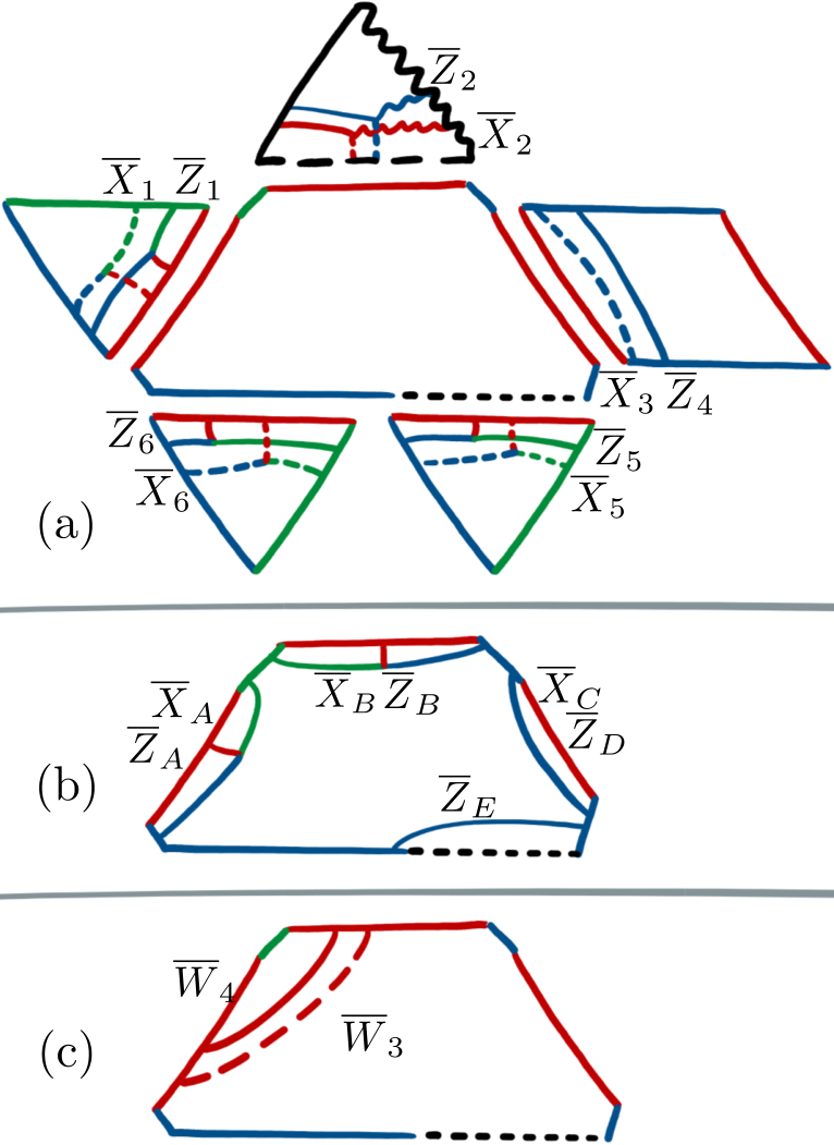
Having discussed the different cases arising in two-patch color code lattice surgery, let us now move onto measurements of Pauli codewords with support on a larger number of patches. General lattice surgery operations are discussed in more detail in Ref. Thomsen et al. 2022. We consider the example shown in Fig. 42. Here, we aim to measure the two Pauli words $W_{1}=\overline{X}_{1}\overline{X}_{2}\overline{X}_{3}\overline{1}_{4}\overline{1}_{5}\overline{1}_{6}$ and $W_{2}=\overline{Z}_{1}\overline{Z}_{2}\overline{X}_{3}\overline{1}_{4}\overline{Z}_{5}\overline{1}_{6}$ which are encoded on five distinct patches of color code. Note, the two Pauli words commute, $\left[W_{1},W_{2}\right]=0$. This implies we are able to measure them at the same time using color code based lattice surgery Thomsen et al. 2022. In the example we find triangular code patches (see Fig. 2) as well as a rectangular code patch (see Fig. 24). Note how the rectangular patch encodes two logical qubits, indexed $4$ and $5$, leading to Pauli words of length $n=6$. To perform the measurement, we introduce an auxiliary patch in the centre, such that it neighbours a boundary of each of the five code patches surrounding it. Furthermore, we choose the boundaries interfacing with code patches that are acted on non-trivially by both $W_{1}$ and $W_{2}$ to be red, and of Pauli type if they are acted on non-trivially only by one of $W_{1}$ and $W_{2}$, such as the Pauli-$X$ boundary interfacing with code patch number $5$. The exception is the boundary interfacing the code patch encoding qubit number $6$, which only gets acted on trivially by both $W_{1}$ and $W_{2}$.

Let us study the auxiliary central patch in its own right. It encodes five logical qubits, which we label based on the logical operators that are supported on the boundaries interfacing the code patches, see Fig. 42 (b). In the lattice surgery protocol, we measure the parity of the depicted logical operators on the auxiliary code patch and the logical operators on the surrounding code patches. In order to measure only $W_{1}$ and $W_{2}$, and no additional information, we initialise the auxiliary code patch using a red temporal boundary, ensuring that it is not initialised in an eigenstate of the depicted logical operators. As shown in Fig. 42 (c), the products of the logical operators in (b) are red strings, namely $W_{3}=\overline{X}_{A}\overline{X}_{B}\overline{X}_{C}$ and $W_{4}=\overline{Z}_{A}\overline{Z}_{B}\overline{Z}_{D}\overline{Z}_{E}$. Thus, initialising with a red temporal boundary initialises the auxiliary code patch in an eigenstate of $W_{3}$ and $W_{4}$. Now, by performing the merging step in the lattice surgery protocol, we measure the products $W_{1}W_{3}$ and $W_{2}W_{4}$. Importantly, the measurements we have performed do not commute with $W_{3}$ and $W_{4}$. Thus, in order to infer $W_{1}$ and $W_{2}$, the values of $W_{3}$ and $W_{4}$ need to be obtained during the splitting step Horsman et al. 2012. This is achieved by reading out the auxiliary code patch using a red temporal boundary.

In the example we have examined, we encounter all types of domain walls. The opaque domain wall between the auxiliary code patch and the triangular code patch encoding logical qubit number $6$ is maintained throughout the protocol. The domain walls between the auxiliary patch and the triangular code patches number $1$ and $2$ are invertible or fully transparent. Note, the domain wall to the patch number $2$ is non-trivial, as it joins a red boundary and a Pauli-$X$ boundary together. The two domain walls between the auxiliary patch and the patch encoding qubits $3$ and $4$ as well as the one encoding qubit number $5$ are semi-transparent. Here, the former is of type (3) in the above discussion, while the latter is of type (2).

With this example we hope to have elucidated how color code lattice surgery can be used to efficiently perform logical gates on a wide range of logical encodings by making use of its rich set of domain walls. This should aid the design of further schemes using unconventional encodings such as the thin color code proposed in Ref. Thomsen et al. 2022, which might be preferable in architectures with biased noise.

To conclude this part of the work, let us summarise how to translate from a circuit describing a quantum computation to a fault-tolerant implementation using the color code. We make our summary using the example presented in Fig. 43, where we make use of all of the features discussed in Secs. IV-VI. The operations we present give rise to a universal set of fault-tolerant logical operations for topological stabiliser codes, where non-Clifford gates are performed with magic state distillation. As we have now elaborated, all of these operations are described, both macroscopically and microscopically, with the unifying language of anyon condensation.

In what follows, we will describe the instantaneous stabiliser group for dynamically condensed color codes. We will explain how the instantaneous stabiliser group is transformed as we make different choices of weight-two edge measurements on the three-colourable lattice.

Dynamically driven codes are described by a series of instantaneous stabiliser groups. Each round of check measurements that are made in the sequence projects the system onto a new instantaneous stabiliser group. Each of the instantaneous stabiliser groups of dynamically condensed color codes $\mathcal{S}_{\texttt{a}}$ are obtained by condensing boson a of the color code. The honeycomb code Hastings and Haah 2021 for example moves, up to a local basis change, through a series of three instantaneous stabiliser groups $\mathcal{S}_{{\texttt{rx}}}$, $\mathcal{S}_{{\texttt{gy}}}$ and $\mathcal{S}_{{\texttt{bz}}}$. In practice we find that we can transform between any two anyon-condensed color codes $\mathcal{S}_{\texttt{a}}$ and $\mathcal{S}_{\texttt{b}}$ provided a and b correspond to bosons of the color code that share neither the same colour or Pauli label.

The deconfined charges of the condensed color code give rise to logical operators of an instantaneous stabiliser group. Specifically, we regard physical string operators that transport deconfined charges over large non-trivial cycles of the lattice as the extensive logical operators. In the case of $\mathcal{S}_{\texttt{rx}}$ the logical operators are generated by the string operators for ry, rz, gx and bx charges.

The edge terms for an instantaneous stabiliser group are stabilisers for the condensed code. They correspond to the string operators that transport the condensed charge. For $\mathcal{S}_{\texttt{rx}}$ this is a weight-two string operator that transports the rx charges in the parent color code model. Indeed, we can generate longer string operators that transport these charges by taking the products of red Pauli-$X$ edge terms that are included in $\mathcal{S}_{\texttt{rx}}$.

We can check that the deconfined charges of the condensed code are identified by fusion with a condensed charge at the microscopic level (see Sec. III.1). We find that logical operators that are identified by condensation are equivalent up to multiplication by edge operators. We depict this equivalence for the case of the condensed code $\mathcal{S}_{\texttt{rx}}$ in Figs. 45 (a) and (b), where we show the equivalence between ry and rz operators, as well as equivalence between gx and bx operators, by multiplication with the edge operators that transport the condensed rx charges.

We can therefore regard string operators ry and rz equivalently as Pauli-$Z$ logical operators, and gx and bx equivalently define Pauli-$X$ logical operators. Likewise, as discussed previously in Sec. III.4, we can identify the deconfined red bosons with, say, an electric charge of the toric code model, ${\texttt{ry}}\simeq{\texttt{rz}}\equiv{\texttt{e}}$, and, similarly, the two deconfined bosons that have a Pauli-$X$ label with a magnetic flux of the toric code; ${\texttt{gx}}\simeq{\texttt{bx}}\equiv{\texttt{m}}$.

Let us now look at how we transform between different instantaneous stabiliser groups in dynamically condensed color codes. We will concentrate on a single transformation to explain how the logical operators are modified under a transformation process, but we note that we can compile a long sequence of transformations of this type. Additionally, we will show how we detect error events from the weight-two check measurements.

As we will see, we can transform between any condensed color codes $\mathcal{S}_{\texttt{a}}$ and $\mathcal{S}_{\texttt{b}}$ provided a and b are bosons that share neither their colour label nor their Pauli label. In other words, we require b to be a confined charge in $\mathcal{S}_{\texttt{a}}$. It is this observation that gives us a generalised construction for dynamically driven codes. As such, without loss of generality, we concentrate on one projection from the initial instantaneous code $\mathcal{S}_{{\texttt{rx}}}$ onto $\mathcal{S}_{{\texttt{gy}}}$. We complete this transformation by measuring all of the Pauli-$Y$ edge operators on green edges. It will be helpful to tabulate the bosonic charges of $\mathcal{S}_{{\texttt{rx}}}$ as follows:

Measuring the green Pauli-$Y$ edge operators to condense the confined gy charges then maps us onto a code with the following bosonic charges

In the former, $\mathcal{S}_{{\texttt{rx}}}$, the rx charges are condensed such that, up to exchange of e and m labels, we can regard the deconfined ry and rz anyons equivalently as electric charges e of the toric code (${\texttt{ry}}\simeq{\texttt{rz}}\equiv{\texttt{e}}$), and similarly gx and bx can both be regarded as deconfined magnetic charges m of the toric code (${\texttt{gx}}\simeq{\texttt{bx}}\equiv{\texttt{m}}$). All other charges are confined. In the latter, the gy anyons are condensed and we have ${\texttt{gx}}\simeq{\texttt{gz}}\equiv{\texttt{m}}$ and ${\texttt{ry}}\simeq{\texttt{by}}\equiv{\texttt{e}}$. Fig. 45 shows the microscopic details of the logical operators as the transformation is made.

Importantly, both $\mathcal{S}_{\texttt{rx}}$ and $\mathcal{S}_{\texttt{gy}}$ share a pair of logical operators. These are string operators for gx and ry charges. This can be read directly by comparing the two boson tables in Eqs. (18) and (19) where we use different colours to correspond to different species of toric-code bosons. One can readily check that both of these boson tables have a common pair of deconfined bosons, that correspond to these anti-commuting logical operators and braid non-trivially with one another. Importantly, this means that logical operators are maintained throughout the transformation and, as such, logical information is preserved. It follows that measuring the gy edge operators does not reveal any logical information from the corresponding string-like logical operators of the deconfined charges. See Fig. 45 for a microscopic illustration.

Let us further emphasise this point that the transformation determines the charge labelling convention for the new code, as this will be important in Sec. VII.3.2 where we consider the transformation of boundary stabilisers for dynamically driven codes. Specifically, we find that the particle identification across the transformation can be read directly from the boson tables of the condensed color codes before and after the transformation. By identifying ry and its corresponding logical operators with, say, the electric charge e in $\mathcal{S}_{\texttt{rx}}$, it follows that the same logical operators must also transport e charges in the transformed code $\mathcal{S}_{\texttt{gy}}$. As such, the ry charge of the transformed code, together with charges that are identified with it under the condensation operation, must also be identified with the e particle. Likewise, by identifying gx with the magnetic particle m in the original code $\mathcal{S}_{\texttt{rx}}$, it follows that gx, and its corresponding string terms that give rise to logical operators, must also be identified with the m particle in the transformed code $\mathcal{S}_{\texttt{gy}}$. We reflect this identification of charges across the transformation using a consistent colouring convention for the two types of deconfined charges in Eqs. (18) and (19). Specifically, we use different colours to correspond to different species of toric-code bosons. In both boson tables in Eqs. (18) and (19), ry is coloured orange in both cases, denoting an e charge, and gx is coloured blue, indicating the identification of this particle with m.

Let us recall the above argument for a specific transformation holds in general for any transformation where a charge that was previously deconfined becomes condensed. If we were to measure the hopping terms of a deconfined charge, such as the red Pauli-$Y$ or Pauli-$Z$ edge terms, or the green or blue edge terms with a Pauli-$X$ label, we would perform a readout. As we have discussed in Sec. IV.1 and Sec. IV.2, condensing a deconfined charge results in the readout of logical information. To summarise, it is essential that the ongoing condensation operation condenses a confined charge of $\mathcal{S}_{\texttt{a}}$ in our construction for dynamically condensed color codes, in order to maintain coherent logical information encoded in the dynamically driven code.

In addition to transforming the logical operators, measuring the green Pauli-$Y$ edge terms also serves to both infer some stabiliser data, and to reinitialise new stabilisers. Measurement of the green edge terms also means that certain stabilisers of $\mathcal{S}_{\texttt{rx}}$ are removed from the system. We will discuss this in more detail for some specific examples in the following section (Sec.VII.2), but let us provide an overview of the mechanics of stabiliser readout with dynamically condensed color codes here. In what follows we explain how the stabiliser group is transformed under a single condensation process, see also Fig. 46.

We are considering the transformation where we project the stabiliser group $\mathcal{S}_{\texttt{rx}}$ onto $\mathcal{S}_{\texttt{gy}}$. Here, we perform green edge measurements that commute with stabilisers on the red and blue plaquettes. As such, the system remains in an eigenstate of all stabiliser generators on red and blue plaquettes. We can also use the green edge measurements to infer the values of the $S^{\texttt{ry}}_{f}$ and $S^{\texttt{by}}_{f}$ operators. Given that we began in an eigenstate of $S^{{\texttt{by}}}_{f}$ we learn its value for a second time. Comparing its new value to its original value allows us to identify errors that have occurred during the interim period, see Fig. 46 (a). This gives rise to a detection cell, introduced in see Sec. II.5 and discussed further in Sec. VII.2.1. In contrast, the stabiliser group $\mathcal{S}_{\texttt{rx}}$ did not include $S^{\texttt{ry}}_{f}$ terms, see Fig. 46 (b). Measuring the green Pauli-$Y$ edge terms therefore initialises the system in eigenstates of these stabilisers, and in turn the $S^{\texttt{rz}}_{f}$ stabiliser given that we maintain an eigenstate of the $S^{\texttt{rx}}_{f}$ stabiliser throughout the transformation. However, given the outcome of this inferred stabiliser measurement is random, these measurements provide no new syndrome data with respect to the red plaquettes.

The transformation also removes stabilisers from the system. The green Pauli-$Y$ edge measurements anti-commute with the $S^{\texttt{gx}}_{f}$ and $S^{\texttt{gz}}_{f}$ stabilisers. These stabilisers are therefore not included in $\mathcal{S}_{\texttt{gy}}$. Indeed, the new stabiliser group only includes $S^{\texttt{gy}}_{f}$ on the green lattice faces. We depict this in Fig. 46 (c).

With the discovery that we can transform between any pair of anyon-condensed color codes from $\mathcal{S}_{\texttt{a}}$ to $\mathcal{S}_{\texttt{b}}$ provided bosons a and b share neither colour nor Pauli labels, we find a new degree of freedom that we can use to design new dynamically driven codes that follow different sequences of check measurements. To this end, we introduce the Floquet color code; a specific example of a dynamically condensed color code (see also Davydova et al. 2022; Bombin et al. 2023 where this code has recently been introduced in independent work on a lattice with periodic boundary conditions).

The Floquet color code follows a sequence of six instantaneous stabiliser groups

see Fig. 47, where we use boson tables to show how the electric and magnetic charges are transformed as the Floquet color code undergoes code deformations.

Let us now describe quantum error correction using the Floquet color code before presenting the numerical results from our threshold simulation. As we have discussed, dynamically condensed color codes maintain canonical pairs of anti-commuting logical operators provided the transformations we use respects the rules that are detailed in the previous subsection (Sec. VII.1). One can check that our sequence respects these results, so let us concentrate on stabiliser measurements.

References

- Dennis et al. (2002) E. Dennis, A. Kitaev, A. Landahl, and J. Preskill, J. Math. Phys. 43, 4452 (2002).
- Kitaev (2003) A. Y. Kitaev, Ann. Phys. 303, 2 (2003).
- Freedman et al. (2000) M. Freedman, M. Larsen, and Z. Wang, Commun. Math. Phys. 227 (2000), 10.1007/s002200200645.
- Levin and Wen (2005) M. A. Levin and X.-G. Wen, Phys. Rev. B 71, 045110 (2005).
- Bombín and Martin-Delgado (2006) H. Bombín and M. A. Martin-Delgado, Phys. Rev. Lett. 97, 180501 (2006).
- Nayak et al. (2008) C. Nayak, S. H. Simon, A. Stern, M. Freedman, and S. Das Sarma, Rev. Mod. Phys. 80, 1083 (2008).
- Gang (2007) W. X. Gang, Quantum field theory of many-body systems: from the origin of sound to an origin of light and electrons (Oxford University Press, Oxford, 2007).
- Brown et al. (2016) B. J. Brown, D. Loss, J. K. Pachos, C. N. Self, and J. R. Wootton, Rev. Mod. Phys. 88, 045005 (2016).
- Raussendorf et al. (2006) R. Raussendorf, J. Harrington, and K. Goyal, Ann. Phys. 321, 2242 (2006).
- Raussendorf and Harrington (2007) R. Raussendorf and J. Harrington, Phys. Rev. Lett. 98, 190504 (2007).
- Bonderson et al. (2008) P. Bonderson, M. Freedman, and C. Nayak, Phys. Rev. Lett. 101, 010501 (2008).
- Bombín and Martin-Delgado (2009) H. Bombín and M. A. Martin-Delgado, J. Phys. A 42, 095302 (2009).
- Fowler (2011) A. G. Fowler, Phys. Rev. A 83, 042310 (2011).
- Horsman et al. (2012) C. Horsman, A. G. Fowler, S. Devitt, and R. V. Meter, New J. Phys. 14, 123011 (2012).
- Brown et al. (2017) B. J. Brown, K. Laubscher, M. S. Kesselring, and J. R. Wootton, Phys. Rev. X 7, 021029 (2017).
- Bombín (2018) H. Bombín, arXiv:1810.09571 (2018), 10.48550/arXiv.1810.09571.
- Brown (2020) B. J. Brown, Science Advances 6, eaay4929 (2020), https://www.science.org/doi/pdf/10.1126/sciadv.aay4929 .
- Zhu et al. (2022) G. Zhu, T. Jochym-O’Connor, and A. Dua, PRX Quantum 3, 030338 (2022).
- Landahl and Ryan-Anderson (2014) A. J. Landahl and C. Ryan-Anderson, arXiv:1407.5103 (2014).
- Thomsen et al. (2022) F. Thomsen, M. S. Kesselring, S. D. Bartlett, and B. J. Brown, arXiv:2201.07806 (2022), 10.48550/arXiv.2201.07806.
- Yoshida (2015) B. Yoshida, Phys. Rev. B 91, 245131 (2015).
- Bridgeman et al. (2017) J. C. Bridgeman, S. D. Bartlett, and A. C. Doherty, Phys. Rev. B 96, 245122 (2017).
- Kesselring et al. (2018) M. S. Kesselring, F. Pastawski, J. Eisert, and B. J. Brown, Quantum 2, 101 (2018).
- Bombin et al. (2012) H. Bombin, G. Duclos-Cianci, and D. Poulin, New J. Phys. 14, 073048 (2012).
- Bhagoji and Sarvepalli (2015) A. Bhagoji and P. Sarvepalli, in 2015 IEEE International Symposium on Information Theory (ISIT) (2015) pp. 1109–1113.
- Kubica et al. (2015) A. Kubica, B. Yoshida, and F. Pastawski, New J. Phys. 17, 083026 (2015).
- Roberts and Williamson (2020) S. Roberts and D. J. Williamson, arXiv:2011.04693 (2020), 10.48550/arXiv.2011.04693.
- Burnell (2018) F. J. Burnell, Ann. Rev. Cond. Matt. Phys. 9, 307 (2018).
- Bais and Slingerland (2009) F. A. Bais and J. K. Slingerland, Phys. Rev. B 79, 045316 (2009).
- Duivenvoorden et al. (2017) K. Duivenvoorden, M. Iqbal, J. Haegeman, F. Verstraete, and N. Schuch, Phys. Rev. B 95, 235119 (2017).
- Iqbal et al. (2018) M. Iqbal, K. Duivenvoorden, and N. Schuch, Phys. Rev. B 97, 195124 (2018).
- Bombín and Martin-Delgado (2008) H. Bombín and M. A. Martin-Delgado, Phys. Rev. B 78, 115421 (2008).
- Gidney (2022) C. Gidney, Quantum 6, 786 (2022).
- Kitaev and Kong (2012) A. Kitaev and L. Kong, Commun. Math. Phys. 313, 351 (2012).
- Kong (2014) L. Kong, Nucl. Phys. B 886, 436 (2014).
- Hastings and Haah (2021) M. B. Hastings and J. Haah, Quantum 5, 564 (2021).
- Haah and Hastings (2022) J. Haah and M. B. Hastings, Quantum 6, 693 (2022).
- Gidney and Newman (2022) C. Gidney and M. Newman, Quantum 6, 813 (2022).
- Davydova et al. (2022) M. Davydova, N. Tantivasadakarn, and S. Balasubramanian, arXiv:2210.02468 (2022).
- Bombin et al. (2023) H. Bombin, D. Litinski, N. Nickerson, F. Pastawski, and S. Roberts, (2023), arXiv:2303.08829.
- Wootton (2022) J. R. Wootton, “Measurements of Floquet code plaquette stabilizers,” (2022).
- Kitaev (2006) A. Kitaev, Ann. Phys. 321, 2 (2006).
- Bombín (2014) H. Bombín, Commun. Math. Phys. 327, 387 (2014).
- Gottesman (1997) D. Gottesman, arXiv:0904.2557 (1997), 10.48550/arXiv.0904.2557.
- Wang et al. (2010) D. S. Wang, A. G. Fowler, C. D. Hill, and L. C. L. Hollenberg, Quant. Inf. Comp. 10, 0780 (2010).
- Landahl et al. (2011) A. J. Landahl, J. T. Anderson, and P. R. Rice, arXiv:1108.5738 (2011), 10.48550/arXiv.1108.5738.
- Sarvepalli and Raussendorf (2012) P. Sarvepalli and R. Raussendorf, Phys. Rev. A 85, 022317 (2012).
- Delfosse and Nickerson (2017) N. Delfosse and N. H. Nickerson, arXiv:1709.06218 (2017).
- Aloshious and Sarvepalli (2018) A. B. Aloshious and P. K. Sarvepalli, Phys. Rev. A 98, 012302 (2018).
- Li (2018) Y. Li, Phys. Rev. A 98, 012336 (2018).
- Tuckett et al. (2019) D. K. Tuckett, A. S. Darmawan, C. T. Chubb, S. Bravyi, S. D. Bartlett, and S. T. Flammia, Phys. Rev. X 9, 041031 (2019).
- Li et al. (2020) J. X. Li, J. M. Renes, and P. O. Vontobel, arXiv:2010.10845 (2020), ISIT45174.2021.9518077.
- Chubb (2021) C. T. Chubb, arXiv:2101.04125 (2021), 10.48550/arXiv.2101.04125.
- Sabo et al. (2021) E. Sabo, A. B. Aloshious, and K. R. Brown, arXiv:2106.08251 (2021), 10.48550/arXiv.2106.08251, arXiv:2106.08251 [quant-ph] .
- Sahay and Brown (2022) K. Sahay and B. J. Brown, PRX Quantum 3, 010310 (2022).
- Wootton (2015) J. R. Wootton, J. Phys. A 48, 215302 (2015).
- Criger and Terhal (2016) B. Criger and B. M. Terhal, Quant. Inf. Comp. 16, 1261 (2016).
- Wang et al. (2003) C. Wang, J. Harrington, and J. Preskill, Ann. Phys. 303, 31 (2003).
- Gidney (2021) C. Gidney, Quantum 5, 497 (2021).
- Strikis et al. (2021) A. Strikis, S. C. Benjamin, and B. J. Brown, arXiv:2111.06432 (2021), 10.48550/arXiv.2111.06432.
- Levin (2013) M. Levin, Phys. Rev. X 3, 021009 (2013).
- Davydov and Simmons (2017) A. Davydov and D. Simmons, J. Alg. 471, 149 (2017).
- Beigi et al. (2011) S. Beigi, P. W. Shor, and D. Whalen, Commun. Math. Phys. 306, 663 (2011).
- Bombín (2010) H. Bombín, Phys. Rev. Lett. 105, 030403 (2010).
- Barkeshli et al. (2019) M. Barkeshli, P. Bonderson, M. Cheng, and Z. Wang, Phys. Rev. B 100, 115147 (2019).
- Bridgeman and Barter (2020) J. C. Bridgeman and D. Barter, Quantum 4, 277 (2020).
- Ellison et al. (2022) T. D. Ellison, Y.-A. Chen, A. Dua, W. Shirley, N. Tantivasadakarn, and D. J. Williamson, PRX Quantum 3, 010353 (2022).
- Delfosse et al. (2016) N. Delfosse, P. Iyer, and D. Poulin, arXiv:1606.07116 (2016), 10.48550/arXiv.1606.07116.
- Benhemou et al. (2022) A. Benhemou, J. K. Pachos, and D. E. Browne, Phys. Rev. A 105, 042417 (2022).
- Eastin and Knill (2009a) B. Eastin and E. Knill, Phys. Rev. Lett. 102, 110502 (2009a).
- Vuillot (2021) C. Vuillot, arXiv:2212.00042 (2021), 10.48550/arXiv.2212.00042.
- Gidney et al. (2021) C. Gidney, M. Newman, A. Fowler, and M. Broughton, Quantum 5, 605 (2021).
- Paetznick et al. (2022) A. Paetznick, C. Knapp, N. Delfosse, B. Bauer, J. Haah, M. B. Hastings, and M. P. da Silva, arXiv:2202.11829 (2022), 10.48550/arXiv.2202.11829, arXiv:2202.11829 [quant-ph] .
- Aasen et al. (2022) D. Aasen, Z. Wang, and M. B. Hastings, Phys. Rev. B 106, 085122 (2022).
- Bombín (2016) H. Bombín, New J. Phys. 18, 043038 (2016).
- Eastin and Knill (2009b) B. Eastin and E. Knill, Phys. Rev. Lett. 102, 110502 (2009b).
- Bravyi and König (2013) S. Bravyi and R. König, Phys. Rev. Lett. 110, 170503 (2013).
- Pastawski and Yoshida (2015) F. Pastawski and B. Yoshida, Phys. Rev. A 91, 012305 (2015).
- Webster and Bartlett (2020) P. Webster and S. D. Bartlett, Phys. Rev. A 102, 022403 (2020).
- Webster et al. (2022) P. Webster, M. Vasmer, T. R. Scruby, and S. D. Bartlett, Phys. Rev. Research 4, 013092 (2022).
- Bravyi and Kitaev (2005) S. Bravyi and A. Kitaev, Phys. Rev. A 71, 022316 (2005).
- Brown (2022) B. J. Brown, arXiv:2207.06428 (2022), 10.48550/arXiv.2207.06428.
- Dong et al. (2008) S. Dong, E. Fradkin, R. G. Leigh, and S. Nowling, Journal of High Energy Physics 2008, 016 (2008).
- Brown et al. (2013) B. J. Brown, S. D. Bartlett, A. C. Doherty, and S. D. Barrett, Phys. Rev. Lett. 111 (2013), 10.1103/physrevlett.111.220402.
- Bonderson et al. (2017) P. Bonderson, C. Knapp, and K. Patel, Ann. Phys. 385, 399 (2017).
- Yoder and Kim (2017) T. J. Yoder and I. H. Kim, Quantum 1, 2 (2017).
- Litinski and von Oppen (2018) D. Litinski and F. von Oppen, Quantum 2, 62 (2018).
- Magdalena de la Fuente et al. (2023) J. C. Magdalena de la Fuente, A. Bauer, and J. Eisert, (2023), arXiv:2302.01835.
- Litinski (2019) D. Litinski, Quantum 3, 12 (2019).
- Litinski et al. (2017) D. Litinski, M. S. Kesselring, J. Eisert, and F. v. Oppen, Phys. Rev. X 7, 031048 (2017).
- Poulin (2005) D. Poulin, Phys. Rev. Lett. 95, 230504 (2005).
- Brown and Williamson (2020) B. J. Brown and D. J. Williamson, Phys. Rev. Res. 2, 013303 (2020).
- Higgott (2021) O. Higgott, arXiv:2105.13082 (2021), 10.48550/arXiv.2105.13082.
- (94) G. repository, https://github.com/BenjaminJamesBrown/FloquetColorCode.
- Bravyi and Kitaev (1998) S. B. Bravyi and A. Y. Kitaev, (1998), 10.48550/arXiv.quant-ph/9811052, quant-ph/9811052.
- Aasen et al. (2020) D. Aasen, D. Bulmash, A. Prem, K. Slagle, and D. J. Williamson, Phys. Rev. Research 2, 043165 (2020).
- Bombín (2015) H. Bombín, New J. Phys. 17, 083002 (2015).
- Breuckmann and Eberhardt (2021a) N. P. Breuckmann and J. N. Eberhardt, PRX Quantum 2, 040101 (2021a).
- Bombin (2010) H. Bombin, Phys. Rev. A 81, 032301 (2010).
- Higgott and Breuckmann (2021) O. Higgott and N. P. Breuckmann, Phys. Rev. X 11, 031039 (2021).
- Steane (1997) A. M. Steane, Phys. Rev. Lett. 78, 2252 (1997).
- Knill (2005) E. Knill, Nature 434, 39 (2005).
- Tuckett et al. (2018) D. K. Tuckett, S. D. Bartlett, and S. T. Flammia, Phys. Rev. Lett. 120, 050505 (2018).
- Bonilla Ataides et al. (2021) J. P. Bonilla Ataides, D. K. Tuckett, S. D. Bartlett, S. T. Flammia, and B. J. Brown, Nature Comm. 12, 2172 (2021).
- Dua et al. (2022) A. Dua, A. Kubica, L. Jiang, S. T. Flammia, and M. J. Gullans, arXiv:2201.07802 (2022), 10.48550/arXiv.2201.07802.
- Srivastava et al. (2022) B. Srivastava, A. Frisk Kockum, and M. Granath, Quantum 6, 698 (2022).
- Miguel et al. (2022) J. F. S. Miguel, D. J. Williamson, and B. J. Brown, arxiv:2203.16534 (2022), 10.48550/arXiv.2203.16534.
- Chamberland et al. (2022) C. Chamberland, K. Noh, P. Arrangoiz-Arriola, E. T. Campbell, C. T. Hann, J. Iverson, H. Putterman, T. C. Bohdanowicz, S. T. Flammia, A. Keller, G. Refael, J. Preskill, L. Jiang, A. H. Safavi-Naeini, O. Painter, and F. G. S. L. Brandão, PRX Quantum 3, 010329 (2022).
- Tuckett et al. (2020) D. K. Tuckett, S. D. Bartlett, S. T. Flammia, and B. J. Brown, Phys. Rev. Lett. 124, 130501 (2020).
- Aliferis and Terhal (2007) P. Aliferis and B. M. Terhal, Quant. Info. Comput. 7, 139 (2007).
- Suchara et al. (2015) M. Suchara, A. W. Cross, and J. M. Gambetta, Quant. Inf. Comput. 15, 997 (2015).
- Ghosh and Fowler (2015) J. Ghosh and A. G. Fowler, Phys. Rev. A 91, 020302 (2015).
- Cong et al. (2017) I. Cong, M. Cheng, and Z. Wang, Phys. Rev. Lett. 119, 170504 (2017).
- Laubscher et al. (2019) K. Laubscher, D. Loss, and J. R. Wootton, Phys. Rev. A 100, 012338 (2019).
- Breuckmann and Eberhardt (2021b) N. P. Breuckmann and J. N. Eberhardt, PRX Quantum 2, 040101 (2021b).
- Chen et al. (2013) X. Chen, Z.-C. Gu, Z.-X. Liu, and X.-G. Wen, Phys. Rev. B 87, 155114 (2013).
- Coste et al. (2000) A. Coste, T. Gannon, and P. Ruelle, Nucl. Phys. B 581, 679 (2000).