Data-driven Science and Machine Learning Methods in Laser-Plasma Physics
Abstract
Laser-plasma physics has developed rapidly over the past few decades as high-power lasers have become both increasingly powerful and more widely available. Early experimental and numerical research in this field was restricted to single-shot experiments with limited parameter exploration. However, recent technological improvements make it possible to gather an increasing amount of data, both in experiments and simulations. This has sparked interest in using advanced techniques from mathematics, statistics and computer science to deal with, and benefit from, big data. At the same time, sophisticated modeling techniques also provide new ways for researchers to effectively deal with situations in which still only sparse amounts of data are available. This paper aims to present an overview of relevant machine learning methods with focus on applicability to laser-plasma physics, including its important sub-fields of laser-plasma acceleration and inertial confinement fusion.
I Introduction
I.1 Laser-Plasma Physics
Over the past decades, the development of increasingly powerful laser systems1, 2 has enabled the study of light-matter interaction across many regimes. Of particular interest is the interaction of intense laser pulses with plasma, which is characterized by strong nonlinearities that occur across many scales in space and time3, 4. These laser-plasma interactions are both of interest for fundamental physics research and as emerging technologies for potentially disruptive applications.
Regarding fundamental research, high-power lasers have for instance been used to study transitions from classical electrodynamics to quantum electrodynamics via radiation reaction, where a particle’s backreaction to its radiation field manifests itself in an additional force5, 6, 7. Recent proposals to extend intensities to the Schwinger limit8, where the electric field strength of the light is comparable to the Coulomb field, could allow the study of novel phenomena expected to occur due to a breakdown of perturbation theory. In an only slightly less extreme case, high-energy density physics (HEDP)9 research uses lasers for the production and study of states of matter that cannot be reached otherwise in terrestrial laboratories. This includes creating and investigating material under extreme pressures and temperatures, leading to exotic states like warm-dense matter10, 11, 12.
Apart from the fundamental interest, there is also considerable interest in developing novel applications that are enabled by these laser-plasma interactions. Two particularly promising application areas have emerged over the past decades, namely the production of high-energy radiation beams (electrons, positrons, ions, X-rays, gamma-rays) and laser-driven fusion.
Laser-plasma acceleration (LPA) aims to accelerate charged particles to high energies over short distances by inducing charge separation in the plasma, e.g. in the form of plasma waves to accelerate electrons or by stripping electrons from thin-foil targets to accelerate ions. The former scenario is called laser wakefield acceleration (LWFA)13, 14, 15. Here a high-power laser propagates through a tenuous plasma and drives a plasma wave which can take the shape of a spherical ions cavity directly behind the laser. The fields within this so-called bubble typically reach around 100 GV/m, allowing LWFA to accelerate electrons from rest to GeV energies within centimeters 16, 17, 18, 19, 20, 21. While initial experiments were single-shot in nature and with significant shot-to-shot variations, the performance of LWFA has drastically increased in recent years. Particularly worth mentioning in this regard are the pioneering works on LWFA at kHz-level repetition rate, starting with an early demonstration in 201322 and in the following mostly developed by J. Faure et al.23, 24 and H. Milchberg’s group25, as well as the day-long stable operation achieved by A. Maier et al.26. As a result of these efforts, typical experimental data sets in publications have significantly increased in size. To give an example, first studies on the so-called beamloading effect in LWFA were done on sets of tens of shots27, whereas newer studies include hundreds of shots28 or most recently thousands of shots29.
Laser-driven accelerators can also function as bright radiation sources via the processes of bremsstrahlung emission30, 31, betatron radiation32, 33 and Compton scattering34, 35, 36. These sources have been used for a variety of proof-of-concept applications37, ranging from spectroscopy studies of warm-dense matter38, over imaging39, 40 to X-ray computed tomography41, 42, 43, 44. It has also recently been demonstrated that LWFA can produce electron beams with sufficiently high beam quality to drive free-electron lasers (FELs) 45, 46, offering an potential alternative driver for next generation light sources 47.
Laser-ion acceleration48, 49 uses similar laser systems as LWFA, but typically operates with more tightly-focused beams to reach even higher intensities. Here the goal is to separate a population of electrons from the ions and then use this electron cloud to strip ions from the target. The ions are accelerated to high energies by the fields that are generated by the charge separation process. This method has been used to accelerate ions to energies of a few tens of MeV/u in recent years. In an alternative scheme, radiation pressure acceleration50, 51, the laser field is used to directly accelerate a target. Even though it uses the same or similar lasers, ion acceleration typically operates at much lower repetition rate because of its thin targets which are not as easily replenished as gas based plasma sources used in LWFA. Recent target design focuses on the mitigation of this issue, for instance using cryogenic jets52, 53, 54, 55 or liquid crystals 56.

Another application of potentially high societal relevance is laser-driven inertial confinement fusion (ICF)57, 58, where the aim is to induce fusion by heating matter to extremely high temperatures through laser-plasma interaction. As the name suggests, confinement is reached via the inertia of the plasma, which is orders of magnitude larger than the thermal energy. To achieve spatially homogenous heating that can penetrate deep into the fusion target, researchers commonly resort to driving the ignition process indirectly. In this method, light is focused into an empty cylindrical cavity, called a hohlraum, which is used to radiate a nearly isotropic blackbody spectrum that extents into the X-ray regime and is subsequently absorbed by the imploding capsule59. Opposed to this, direct-drive methods aim to directly drive the thermonuclear fusion process60. In this case, the laser is focused directly onto the fuel capsule. Direct-drive poses some challenges that are not present in indirect-drive schemes. For instance, the light has to penetrate through the high-density plasma shell surrounding the capsule and the illumination is less homogeneous, because of which the compressed target can be subject to large hydrodynamic instabilities. Advanced ignition schemes aim to separate compression of the thermonuclear fuel from triggering the ignition process. Examples are fast ignition61, which uses the high-intensity laser pulse to directly heat the compressed and dense fusion target, or shock ignition62, which uses a shock wave to compress the target. Recently, a first ICF experiment at the National Ignition Facility has reported reaching the burning-plasma state via combination of indirect-drive with advanced target design63. This breakthrough has re-enforced scientific and commercial interest in ICF, which is now also pursued by a number of start-up companies.
I.2 Why data-driven techniques?
In recent years, data-driven methods and machine learning have been applied to a wide range of physics problems64, including for instance quantum physics65, 66, particle physics67, condensed matter physics68, electron microscopy69 and fluid dynamics70. In comparison, its use in laser-plasma physics is still in its infancy and is curiously driven by both data abundance and data scarcity. Regarding the former, fast developments in both laser technology71 and plasma targetry72, 73, 74, 75 nowadays permit operation of laser-plasma experiments - in particular laser-plasma accelerators - at Joule-level energies and multi-Hz to kHz repetition rates 76, 77, 78, 79, 80. The vast amounts of data generated by these experiments can be used to develop data-driven models, which are then employed in lieu of conventional theoretical or empirical approaches, or to augment them. In contrast, laser systems used for inertial fusion research produce MJ-level laser pulses and operate at repetition rates as low as one shot per day. With such a sparse amount of independent experimental runs, data-driven models are used to extract as much information as possible from the existing data or combine them with other information sources such as simulations.
The success of all of the above applications depend on the precise control of a complex nonlinear system. In order to optimize and control the process of laser-plasma interaction, it is essential to understand the underlying physics and to be able to model the complex plasma response to an applied laser pulse. However, this is complicated by the fact that it is a strongly nonlinear, multi-scale, multi-physics phenomenon. While analytical and numerical models have been essential tools for understanding laser-plasma interactions, they have several limitations. Firstly, analytical models are often limited to low-order approximations and therefore cannot accurately predict the behavior of complex laser-plasma systems. Secondly, accurate numerical simulations require immense computational resources, often millions of core hours, which limits their use for optimizing and controlling real-world laser-plasma experiments. In addition, the huge range of temporal and spatial scales mean that in practice many physical processes (ionisation, particle collisions, etc.) can only be treated approximately in large scale numerical simulations. Because of this, one active area of research is to automatically extract knowledge from data in order to build faster computational models that can be used for prediction, optimization, classification and other tasks.
Another important problem is that the diagnostics employed in laser-plasma physics experiments typically only provide incomplete and insufficient information about the interaction and key properties must be inferred from the limited set of available observables. Such inverse problems can be hard to solve, especially when some information is lost in the measurement process and the problem becomes ill-posed. Modern methods, such as compressed sensing and deep learning are strong candidates to facilitate the solution of such problems and thus retrieve so-far elusive information from experiments.
The goal of this review is to summarize the rapid, recent developments of data-driven science and machine learning in laser-plasma physics, with particular emphasis on laser-plasma acceleration, and to provide guidance for novices regarding the tools available for specific applications. We would like to start with a disclaimer that the lines between machine learning and other methods are often blurred11 1 For instance, deep learning is a subfield of machine learning where deep neural networks are used, and this term is nowadays often used interchangeably with neural networks. Similarly, data-driven science is sometimes used instead of machine learning, but also includes a variety of methods from computer science, applied mathematics and statistics, as well as data science, which is a field in itself. Even within itself, machine learning is a heavily segmented research field, whose community can famously be divided into five “tribes”, namely symbolists, connectionists, evolutionists, Bayesians and analogizers. Each of these groups has pioneered different tools, all of which have in recent years experienced resurgence in popularity. The arguably most popular branch is connectionism, which focuses on the use of artificial neural networks. However, some challenges seen in laser-plasma physics require different approaches and, for instance, Bayesian optimization has recently drawn considerable research interest. Another line of division is often drawn between supervised and unsupervised methods. While supervised methods are usually trained from known data sets to build a model that can classify new data, unsupervised methods attempt to find some structure in the data without such pre-existing knowledge. Alternatively, one can distinguish between online and batch methods, where the former learn from data as it becomes available, and can therefore be used in an experimental setting, while the latter require access to the full dataset before learning can begin. Yet another important distinction can be made between parametric and non-parametric methods, where the former rely on a set of parameters that is fixed and known in advance, while the latter do not make this assumption, but learn the model parameters from the data.. Given the multitude of often competing subdivisions, we have chosen to organize this review based on a few broad classes of problems, which we believe to have highest relevance for laser-plasma physics and its applications. These problems are modeling & prediction (Section II), inverse problems (Section III), optimization (Section IV), unsupervised learning for data analysis (Section V) and last, image analysis with supervised learning techniques (Section VI). Partial overlap between these applications and the tools used is unavoidable and is where possible indicated via cross-references. This is particularly true in the case of neural networks, which have found a broad usage across applications. Each section includes introductions to the most common techniques that address the problems outlined above. We explicitly include what can be considered as “classical” data-driven techniques in order to provide a better context for more recent methods. Furthermore, examples for implementations of specific techniques in laser-plasma physics and related fields are highlighted in separate text boxes. We hope that these will help the reader to get a better idea which methods might be most adequate for their own research. An overview of the basic application areas is shown in Fig. 1.
To maintain brevity and readability, some generalizations and simplifications are made. For detailed descriptions and strict definitions of methods, the reader is kindly referred to the references given throughout the text. Furthermore, we would like to draw the reader’s attention to some recent reviews on the application of machine learning techniques in the related fields of plasma physics82, 83, 84, ultrafast optics85, and high-energy-density physics86.
II Modeling & prediction
Many real-life and simulated systems are expensive to evaluate in terms of time, money or other limited resources. This is particularly true for laser-plasma physics, which either hinges on the limited access to high-power laser facilities or requires high-performance computing to accurately model the ultra-fast laser-plasma interaction. It is therefore desirable to find models of the system, sometimes-called digital twins87, which are comparatively cheap to evaluate and whose predictions can be used for extensive analyses. In engineering and especially in the context of model-based optimization (see Section IV) such lightweight models are often referred to as surrogate models. Reduced order models feature less degrees of freedom than the original system, which is often achieved using methods of dimensionality reduction (see Section V.3).
The general challenge in modeling is to find a good approximate for the real system based on only a limited number of examples , the training data. Here is an -sized set of vector-valued input parameters and are the corresponding outputs. To complicate things further, any real measurement will be subject to noise, so has to be interpreted as a combination of the true value and some random noise contribution. Another complication arises from having imperfect or unrepeatable controllers for the input parameters . This can result in having different output values for the same set of input parameters.
The predictive models discussed in Section II.1 below are mostly used to interpolate between training data, whereas the related problem of forecasting (Section II.2) explicitly deals with the issue of extrapolating from existing data to new, so-far unseen data. In Section II.3 we briefly discuss how models can be used to provide direct feedback for laser-plasma experiments.
II.1 Predictive models
In this section, we describe some of the most common ways to create predictive models, starting with the “classic” approaches of spline interpolation and polynomial regression, before discussing some modern machine learning techniques.

II.1.1 Spline Interpolation
The simplest way of constructing a model for a system, be it a real-world system or some complex simulation, is to use a set of training points and to predict that every unknown position will have the same value as the nearest neighboring training point (see Fig. 2a). A straightforward extension with slightly higher computational requirements is to connect the training points with straight lines, resulting in a piecewise linear function. Both methods however, are not continuously differentiable, and for instance less suited for the integration of the model into an optimization process (see Section IV). A more advanced approach to interpolating the training points is to use splines (see Fig. 2b), which require the piecewise-interpolated functions to agree up to a certain derivative order. For instance, cubic splines are continuously differentiable up to the second derivative. While higher-order spline interpolation works well in one-dimensional cases, it becomes increasingly difficult in multi-dimensional settings. Furthermore, the interpolation approach does not allow for incorporating uncertainty or stochasticity, which is present in real-world measurements. Therefore, it will treat noise components as a part of the system, including for instance outliers.
II.1.2 Regression
In some specific cases the shortcomings of interpolation approaches can be addressed by using regression models. For instance, simple systems can often be described using a polynomial model, where the coefficients of the polynomial are determined via a least-squares fit (see Fig. 2c), i.e. minimising the sum of the squares of the difference between the predicted and observed data. The results are generally improved by including more terms in the polynomial but this can lead to overfitting – a situation where the model describes the noise in the data better than the actual trends, and consequently will not generalise well to unseen data. Regression is not restricted to polynomials, but may use all kinds of mathematical models, often motivated by a known, underlying physics model. Crucially, any regression model requires the prior definition of a function to be fitted, thus posing constraints on the relationships that can be modeled. In practice this is one of the main problems with this approach, as complex systems can scarcely be described using simple analytical models. Before using these models, it is thus important to verify their validity, e.g. using a measure for the goodness of fit such as the correlation coefficient , the test or the mean-square error (MSE).
II.1.3 Probabilistic models
The field of probabilistic modeling relies on the assumption that the relation between the observed data and the underlying system is stochastic in nature. This means that the observed data are assumed to be drawn from a probability distribution for each set of input parameters to a generative model. Inversely, one can use statistical methods to infer the parameters that best explain the observed data. We will discuss such inference problems in more detail in the context of solving (ill-posed) inverse problems in Section III.2.
Probabilistic models can generally be divided into two methodologies, frequentist and Bayesian. At the heart of the frequentist approach lies the concept of likelihood, , which is the probability of some outcomes or observations given the model parameters (see e.g. Ref.88 for an introduction). A model is fitted by maximum likelihood estimation (MLE), which means finding the model parameters that maximize the likelihood, . When observations are independent, the probability of observing is the product of the probabilities of each observation, . As sums are generally easier to handle than products, this is often expressed in terms of the log-likelihood function that is given by the sum of the logarithms of each observation’s probability, i.e.
| (1) |
Probabilities have values between 0 and 1, so the log-likelihood is always negative and, the logarithm being a strictly monotonic function, minimizing the log-likelihood maximizes the likelihood
| (2) |
The optimum can be found using a variety of optimization methods, e.g. gradient descent, which are described in more detail in Section IV. A simple example is the use of MLE for parameter estimation in regression problems. In case the error is normally distributed this turns out to be equivalent to the least squares method we discussed in the previous section.
The MLE is often seen as the simplest and most practical approach to probabilistic modeling. One advantage is that it does not require any a priori assumptions about the model parameters, but only about the probability distributions of the data. But this can also be a drawback if useful prior knowledge of the model parameters is available. In this case one would turn to Bayesian statistics. Here one assesses information about the probability that a hypothesis about the parameter values is correct given a set of data . In this context the probabilistic model is viewed as a collection of conditional probability densities for each set of observed data , with the aim of finding the posterior distribution , i.e. the probability of some parameters given the data observations. This can be done by applying Bayes’ rule,
| (3) |
where is known from above as likelihood function and denotes the prior distribution, i.e. our a priori knowledge about the parameters before we observe any data . The denominator, , is called the evidence and ensures that both sides of Eq. 3 are properly normalized by integrating over all possible input parameters . Once the posterior distribution is known, we can maximize it and get the maximum a posteriori (MAP) estimate
| (4) |
As mentioned above, a particular strength of the Bayesian approach is that we can encode a priori information in the prior distribution. Taking the example of polynomial regression, we could for instance set a prior distribution for the regression coefficients that favors small coefficients, thus penalizing high-order polynomials. Another advantage of using the Bayesian framework is that one can quantify the uncertainty in the model result. This is particularly simple to compute in the special case of Gaussian distributions and their generalization, Gaussian processes, which we are going to discuss in the next section.

II.1.4 Gaussian process regression
A popular version of Bayesian probabilistic modeling is Gaussian process (GP) regression 89, 90. This kind of modeling was pioneered in geostatistics in the context of mining exploration and is historically also referred to as kriging, after the South African engineer Danie G. Krige, who invented the method in the 1950s. Conceptually, one can think of it as loosely related to the spline interpolation method, as it is also locally “interpolates” the training points. Compared to splines and conventional regression methods, kriging has a number of advantages. Being a regression method, kriging can deal with noisy training points as seen in experimental data. At the same time, the use of Gaussian processes involves minimal assumptions and can in principle model any kind of function. Last, the “interpolation” is done in a probabilistic way, i.e. a probability distribution is assigned to the function values at unknown positions (see Fig. 2d). This allows for quantifying the uncertainty of the prediction. These features make kriging an attractive method for the construction of surrogate models for complex systems, for which only a limited number of the function evaluations is possible, e.g. due to the long runtime of the system or the high costs of the function evaluations. GP regression forms the backbone of most implementations of Bayesian optimization, which we will discuss in Section IV.5, including examples for potential use cases.
Mathematically speaking a Gaussian process is an infinite collection of normal random variables, where each finite subset is jointly normally distributed. The mean vector and covariance matrix of the multivariate normal distribution are thereby generalised to the mean function and the covariance function respectively, where we use the short-hand notation to denote the function inputs as a vector of real numbers.
A Gaussian process can be written in the form:
| (5) |
denoting that the random function follows a Gaussian process with mean function and covariance function .
The mean function is defined as the expectation of the GP, i.e. , whereas the covariance function is defined as . Note that in the special case of constant mean function and a constant diagonal covariance function , the Gaussian process simply reduces to a set of a normal random variable with zero mean and variance commonly referred to as white noise. The covariance function is also referred to as the kernel. Its value at locations and is proportional to the correlation between the function values and . A common choice for the covariance function is the squared exponential function, also known as the radial basis function (RBF) kernel
| (6) |
where is the length scale parameter, which controls the rate at which the correlation between and decays. This kernel hyperparameter can usually be optimized by using the training data to minimize the log marginal likelihood.
It is possible to encode prior knowledge by choosing a specialized kernel that imposes certain restrictions on the model. A variety of such kernels exist. For instance, the periodic kernel (also known as exp-sine-square kernel) given by
| (7) |
with the Euclidean distance , length scale and periodicity as free hyperparameters, is particularly suitable to model systems that show an oscillatory behavior.
A useful property of kernels is the generation of new kernels through addition or multiplication of existing kernels 91. This property provides another way to leverage prior information about the form of the function to increase the predictive accuracy of the model. For instance, measurement errors incorporated into the model by adding a Gaussian white noise kernel, as for instance done in Fig. 2.
Fig. 3 visualizes the covariance functions and their influence on the result of Gaussian process regression. This includes correlation matrices for the three covariance functions discussed above (white noise, RBF and periodic kernels). Once the mean and the covariance functions are fully defined, we can use training points for regression, i.e. fit the Gaussian process and kernel parameters to the data and obtain the posterior distribution, see right panel of Fig. 3.
II.1.5 Decision trees and forests
A decision tree is a general-purpose machine learning method that learns a tree-like model of decision rules from the data to make predictions92. It works by splitting the dataset recursively into smaller groups, called nodes. Each node represents a decision point, and the tree branches out from the node according to the decisions that are made. The leaves of the tree represent the final prediction. This can be either a categorical value in classification tasks (see Section VI) or a numerical value prediction in regression tasks. An advantage of this approach is that it can learn non-linear relationships in data without having to specify them.
To generate a decision tree one starts at the root of the tree and determines a decision node such that it optimizes an underlying decision metric like the mean squared error in regression settings or entropy and information gain in a classification setting. At each decision point the data set is split and subsequently the metric is re-evaluated for the resulting groups, generating the next layer of decision nodes. This process is repeated until the leaves are reached. The more layers decision layers are used, called the depth of the tree, the more complex relationships can be modeled.
Decision trees are easy to implement and can provide accurate predictions even for large data sets. However, with increasing number of decision layers they may become computationally expensive and may overfit the data, the latter being in particular a problem with noisy data. One method to address overfitting is called pruning, where branches from the tree that do not improve the performance are removed. Another effective method is to use decision-tree-based ensemble algorithms instead of a single decision tree.
One example of such algorithm is the random forest, an ensemble algorithm that uses bootstrap aggregating or bagging to fit trees to random subsets of the data and the predictions of individually fitted decision trees are combined by majority vote or average to obtain a more accurate prediction. Another type of ensemble algorithms is boosting, where the trees are trained sequentially and each tries to correct its predecessor. A popular implementation is AdaBoost93 where the weights of the samples are changed according to the success of the predictions of the previous trees. Gradient boosting methods94, 95 also use the concept of sequentially adding predictors, but while AdaBoost adjust weights according to the residuals of each prediction, gradient boosting methods fit new residual trees to the remaining differences at each step (see Fig. 5 for an example).
Compared to other machine learning algorithms, a great advantage of a decision tree is its explicitness in data analysis, especially in nonlinear high-dimensional problems. By splitting the dataset into branches, the decision tree naturally reveals the importance of each variable regarding the decision metric. This is in contrast to “black-box” models, such as those created by neural networks, which must be interpreted by post hoc analysis.
II.1.6 Neural networks
Neural networks offer a versatile framework for fitting of arbitrary functions by training of a network of connected nodes or neurons, which are loosely inspired by biological neurons. In the case of a fully connected neural network, historically called a multilayer perceptron, the inputs to one node are the outputs of all of the nodes from the preceding layer. The very first layer is simply all of the inputs for the function to be modelled, and the very last layer is the function outputs. One of the very attractive properties of neural networks is the capacity to have many outputs and inputs, each of which can be multi-dimensional. The weighting of each connection and the bias for each node are the parameters of the network, which must be trained to provide the best approximation of the function to be modelled. Each node gets activated depending on both weights and biases according to a pre-defined activation function. The non-linear properties of activation functions are widely seen as the key property to allow neural networks to model arbitrary functions and achieve general learning properties.
One of the simplest, but also most common activation functions is the rectified linear unit (ReLU), which is defined as
| (8) |
The function argument is the sum of the weights of incoming connections, multiplied with their values , and the bias of the node. The ReLU function is easy to compute, and it has the main advantage that it is linear for , which greatly simplifies the gradient calculation in training (see next paragraph). Drawbacks are that it is not differentiable at , it is unbounded, and since it yields a constant value below , it has the potential to produce “dead” neurons. The last issue is solved in the so-called leaky ReLU, which uses a reduced gradient for , giving an output of where . Other common activation functions include the logistic or sigmoid function, , and the hyperbolic tangent function function, .
The training is performed iteratively by passing corresponding input-output pairs to the network and comparing the true outputs to those given by the network to calculate the loss function. This is often chosen to be the mean squared error (MSE) between the model output and the reference from the training data, but many other types of loss functions are also used (see Section IV.1.1) and the choice of loss function strongly affects the model’s training. The loss is then used to modify the weights and biases via an algorithm known as “back-propagation”101. Here the gradient of the loss function is calculated with respect to the weights and biases via the chain rule. One can then optimize the parameters using for instance stochastic gradient descent (SGD) or Adam (Adaptive moment estimation) 102.
A number of hyperparameters are used to control the training process. Typical ones include: the number of epochs - the number of times the model sees each data point; the batch size - the number of data points the model sees before updating its gradients; and the learning rate - a factor determining the magnitude of the update to the gradient. Each factor can have a critical effect on the training of the model.
In the training process, the weights and biases are optimized in order to best approximate the function for converting the the inputs into the corresponding outputs. The resulting model will yield an approximation for the unknown function . However, learning via this method only optimizes how well the model reproduces the training data and, in the worst case, the network essentially “memorizes” the training data, and learns little about the desired function . To quantify this, a subset of the of data is kept separate and used solely for validating the model. Ideally, the loss should be similar on both training and validation data, and if the model has significant smaller loss on the training data than the validation set it is said to overfit, which signifies that the model has learnt the random noise of the training set. The validation loss thus quantifies how well this model generalizes and with it, how useful it is for predictions on unseen data.
Common methods to combat overfitting include early stopping, i.e. terminating the training process once the validation loss stagnates; or the use of dropout layers to randomly switch off some fraction of the network connections for each batch of the training process, thereby preventing the network from learning random noise by reducing its capacity. A further approach is to incorporate variational layers into the network. In these layers, pairs of nodes are used which represent the mean and standard deviation of a Gaussian distribution. During training, output values are sampled from this distribution and then passed on the subsequent layers, thereby requiring the network to react smoothly to these small random variations to achieve a small training loss. Both dropout layers and variational layers provide regularization which smooths the network response and prevents single nodes from dominating, resulting in improved interpolation performance and better validation loss 103, 104 (see Section III.3 for a brief, general explanation of regularization).
Beyond the classical multilayer perceptron network, there exists a plethora of different neural network architectures, as partially illustrated in Fig. 6, which are suited to different tasks. In particular, convolutions layers, which extract relevant features from 1D and 2D by learning suitable convolution matrices, are commonly used in the analysis of physical signals and images. Architecture selection and hyperparameter tuning is a central challenge in the implementation of neural networks, and is often performed by an additional machine-learning algorithm, e.g. using Bayesian optimization (see Section IV.5).
The great strength of neural networks is their flexibility and relatively straightforward implementation, with many openly accessible software platforms available to choose from. However, trained networks are effectively “black-box” functions, and do not, in their basic form, incorporate uncertainty quantification. As a result, the networks may make over-confident predictions about unseen data while giving no explanation for those predictions, leading to false conclusions. Various methods exist for incorporating uncertainty quantification into neural networks (see for example 105), such as by including variational layers (discussed above) and training an ensemble of networks on different training data subsets. There are several approaches to try and make neural network models explainable and a review of methods for network interpretation is for instance given by Montavon et al.106.
Another strength of neural networks is that the performance of a model on a new task can be improved by leveraging knowledge from a pre-trained model on a related task. This so-called transfer learning is typically used in scenarios where it is difficult or expensive to train a model from scratch on a new task, or when there is a limited amount of training data available. For example, transfer learning has been used to successfully train models for image classification and object detection tasks (see Section VI), using pre-trained models that have been trained on large image datasets such as ImageNet 107. In the context of laser-plasma physics, transfer learning could be used to improve the performance of a neural network by leveraging knowledge from a pre-trained model that has been trained on data from previous experiments or simulations.

II.1.7 Physics-informed machine learning models
The ultimate application of machine learning for modeling physics systems would arguably be to create an “artificial intelligence physicist”, as coined by Wu and Tegmark115. One prominent idea at the backbone of how we build physical models is Occam’s razor, which states that given multiple hypotheses, the simplest one which is consistent with the data is to be preferred. In addition to this guiding principle, it is furthermore assumed that a physical model can be described using mathematical equations. A program should therefore be able to automatically create such equations, given experimental data. While a competitive AI physicist is still years away22 2 Recently there has also been astonishing progress in the area of large language models such as generative pre-trained transformer (GPT) modelsradford2018improving. Very similar to forecasting networks discussed in Section II.2.3, these use an attention mechanism to predict the next token (word, etc.) following input provided by the user. It was found that large models ( parameters) become increasingly capable with sufficient training, e.g. gaining the ability to do basic math and to write code, including to some claims first hints at artificial general intelligencebubeck2023sparks., first steps have been undertaken in this direction. For instance, in 2009 Schmidt et al.117 presented a genetic algorithm approach (Section IV.4) that independently searched and identified governing mathematical representations such as the Hamiltonian from real-life measurements of some mechanical systems. More recently, research has concentrated more on the concept of Occam’s razor and the underlying idea that the “simplest” representation can be seen as the sparsest in some domain. A key contribution was SINDy (Sparse Identification of Nonlinear Dynamics), a framework for discovering sparse nonlinear dynamical systems from data118. As in compressed sensing (Section III.4), the sparsity constraint was imposed using an -norm regularization, which results in the identification of the fewest terms needed to describe the dynamics.
An important step towards combining physics and machine learning was undertaken in physics-informed neural networks (PINNs)119. A PINN is essentially a neural network that uses physics equations, which are often described in form of ordinary differential equations (ODEs) or partial differential equations (PDEs), as a regularization to select a solution that is in agreement with physics. This is achieved by defining a custom loss function that includes a discrepancy term, the residuals of the underlying ODEs or PDEs, in addition to the usual data-based loss components. As such, solutions that obey the selected physics are enforced. In contrast to SINDy, there is no sparsity constraint imposed on the network weights, meaning that the network could still be quite complex. Early examples of PINNs were published by Raissi et al. 120, 121, 122, 123 and Long et al.124 in 2017. Since then, the architecture has been applied to a wide range of problems in the natural sciences, with a quasi-exponential growth in publications125. Applications include for instance (low-temperature) plasma physics, where PINNs have been successfully used to solve the Boltzmann equation126, or quantum physics, where PINNs were used to solve the Schrödinger equation of a quantum harmonic oscillator127. The work by Stiller et al.127 uses a a scalable neural solver that could possibly also be extended to solve e.g. the Vlasov-Maxwell system governing laser-plasma interaction.
II.2 Time series forecasting
A related problem meriting its own discussion is time series forecasting. While models in the previous section are based on interpolation or regression within given data points, forecasting explicitly deals with the issue of extrapolating parameter values to the future based on prior observations. Most notably this includes modeling of long-term trends (in a laser context often referred to as drifts) or periodic oscillations of parameters and short-term fluctuations referred to as jitter.
If available, models may also use covariates, auxiliary variables that are correlated to the observable, to improve the forecast. These covariates may even extend into the future (seasonal changes being the traditional example in economic forecasting).
In this section we are going to first discuss two common approaches to time series forecasting, autoregressive models and state-space models, followed by a discussion of modern techniques based on neural networks. Note that the modeling approaches presented in the preceding section may also be used, to some extend, to extrapolate data. We are not aware of any recent examples on time series forecasting in the context of laser-plasma physics. However, we feel that the topics merits inclusion in this overview as implementations are likely in the near future, e.g. for laser stabilization purposes.
II.2.1 Classical models
To model a time series one usually starts with a set of assumptions regarding its structure i.e. the interdependence between values at different times. A simple, approximate assumption is that the observed values in a discrete-time time series are linearly related. An important, wide-spread class of such models are so-called autoregressive models which assert that the next value in a time series is given as a linear function of the prior values . Additionally, each value is assumed to be corrupted by additive white noise , representing e.g. measurement errors or inherent statistical fluctuations of the underlying process, which endows the models with stochasticity. In its most common form the autoregressive model of order , denoted by , is defined via the recurrence relation
| (9) |
where are the model’s parameters to be estimated. In this form the problem of finding the model’s parameters is a linear regression problem that can be solved via the least squares method
| (10) |
In another approach we might assume that the next value is instead given by a linear combination of (external) statistical fluctuations, sometimes called shocks, from the past points in time, again encoded in white noise terms . The corresponding model, called the moving average model and denoted by , is defined as
| (11) |
where is the mean of the time series.
The parameters of the moving average process cannot be inferred by linear methods like least squares, but have to be estimated by means of maximum likelihood methods.
Contrary to the model, which is only stationary33 3 A time series is said to be strictly stationary, given the joint cumulative distribution , if . Correspondingly all moments of the joint distribution are invariant under time translation. If this invariance only holds for the first two moments (mean, variance) the time series is said to be (weakly) stationary. for certain parameters , the model is always (strictly) stationary per definition. Put loosely, stationarity can be understood as the stochastic properties (mean, variance, …) of the time series being constant over time.
Another distinction between the autoregressive and the moving average model is how far into the future the effects of statistical fluctuations (shocks) are propagated. In the moving average model the white noise terms are only propagated steps into the future, while in the autoregressive model the effects are propagated infinitely far into the future. This is because the white noise terms are part of the prior values which themselves are part of future values in Eq. 9.
If the time series in question cannot be explained by the or the model alone, both models can be combined into what is called an autoregressive-moving-average model, denoted by
| (12) |
Note that for the special cases of and the reduces to the and respectively.
When fitting autoregressive models special care should be taken that the time series to be modelled is stationary before fitting, otherwise spurious correlations are introduced. Spurious correlations are apparent correlations between two or more time series that are not causally related thereby potentially leading to fallacious conclusions as warned of in the well-known adage ”correlation does not imply causation”.
If the time series is non-stationary in general but stationary with respect to its mean, i.e. the variations relative to the mean value are stationary, it might be possible to transform it into a stationary time series. For this we introduce a new series by differencing the original series times, where we defined the differencing operator . Applying the differencing operator once (), for example, removes a linear trend from , applying it twice removes a quadratic trend and so forth. If is stationary after differencing -times it can be readily modelled by Eq. 12 which leads us to the autoregressive-integrated-moving-average model
| (13) |
Note that in contrast to the model in Eq. 12 the time series appearing here is a -times differenced version of the original series . Further extensions that will only be noted here for completeness here are seasonal ARIMA models called SARIMA that allow the modelling of time series that exhibit seasonality (periodicity) and exogeneous ARIMA models called ARIMAX that allow the modelling of time series that are influenced by a separate, external time series. Both extensions can be combined to yield the so-called SARIMAX model which is general enough to cover a large class of time series problems. However we are still in any case limited to problems in which the time series is generated by a linear stochastic process. To cover more general, non-linear problems we introduce state-space models.
II.2.2 State-Space Models
State-space models (SSMs) offer a very general framework to model time series data129. In this framework, presuming that the time series is based on some underlying system, it is assumed that there exists a certain true state of the system of which we observe a value subject to measurement noise. The true state , usually inaccessible and hidden to us, and the observed state are modeled by the state equation and the observation equation respectively. A prominent example of SSMs in Machine Learning are Hidden Markov models (HMMs)130, in which the hidden state is modeled as a Markov process. In general there are no restrictions on the functional form of the state and observation equations, however, the most common type of SSMs are linear Gaussian SSMs, also referred to as dynamic linear models, in which the state and observation equations are modeled as linear equations and the noise is assumed Gaussian. The prototypical example of such linear Gaussian SSMs is the Kalman filter131, ubiquitous in control theory, robotics and many other fields132, including for instance adaptive optics133 and particle accelerator control134. The term ”filter” originates from the fact that it filters out noise to estimate the underlying state of a system. The state equations can be written as
| (14) |
where the system noise and observation noise are sampled from a normal distribution . Note that the separation of these two noise terms differs from the so-far discussed models. This permits the modelling of systems that are driven by noise, while also accounting for observation noise of possibly differing amplitude. Another difference is the addition of a second process , commonly called the control input in signal processing, which is a deterministic external process driving the system state. This permits the modelling of systems with known external inputs (e.g. a controller-driven motor) or with known deterministic drivers (e.g. system temperature). Note that we can recover the autoregressive models discussed earlier as a special case of the Kalman filter. For example, the process is obtained by setting , , , and . For a more detailed discussion on Kalman filters we refer the interested reader to the literature135. Other (non-linear) ways to perform inference in state-space models exist, for instance using sequential Monte-Carlo estimation136.
II.2.3 Forecasting networks
While predictions based on autoregression or state-space models can suffice for many applications, the non-linear nature of neural networks can be harnessed to model time series with complex, non-linear dependencies137, 138. A particularly relevant architecture are recurrent neural networks (RNNs). These are similar to the “traditional” neural networks we discussed in Section II.1.6, but they have a “memory” that allows them to retain information from previous inputs. This is implemented in a somewhat similar way to the linear recurrence relations discussed in the previous sections, with a key difference being that the state of RNNs is updated according to an arbitrary nonlinear function. The current state is calculated from the previous states through the recurrence equation
| (15) |
where is a nonlinear activation function, a matrix of recurrent weights, and is a bias vector. This equation allows the update to each element of the current state vector, , to be be dependent on the whole of the previous state vector, . The output of the network is calculated from the current state through the output equation
| (16) |
where contains the output weights and is another bias vector. Thus, the entire network state is updated from the previous state through a recurrent equation, and the current output is calculated from the current state through an output equation. The network state therefore contains all previous information about the time series. However, as the network state is updated by a simple multiplication of the weights with the previous state , the so-called vanishing gradient problem may occur139, 140. This problem is solved in a seminal work by Hochreiter 141, who introduced a special type of RNNs, the long short-term memory (LSTM) network. In contrast to the simple update equation of RNNs, LSTMs use a special type of memory cell that can learn long-term dependencies. This includes a so-called forget gate to update the previous state to the current state :
| (17) |
where denotes the element-wise Hadamard product, . Additionally, the LSTM uses two more gates, the input gate and output gate , where the latter is used to calculate the hidden state from the previous hidden state via . The three gates , and are calculated from the current input , the previous hidden state , and the previous gate states , , and using individually set weights and biases. The gates determine how much of the previous state and the current hidden state is used to calculate the current state . The output of the LSTM network is then calculated from the current state through the same output equation, Eq. 16, as used in the RNN. Despite it being introduced in the early 1990s, the LSTM architecture remains one of the most popular network architectures for predictive tasks to date.
A more recently introduced type of neural network that can learn to interpret and generate sequences of data are transformers. Transformers are similar to RNNs, but instead of processing the time series in a sequential manner, they use a so-called attention mechanism142 to capture dependencies between all elements of the time series simultaneously and thus, focus on specific parts of an input sequence. Assuming again a time series , a transformer maps each point to a representation using a linear layer, e.g., . The transformer network then calculates a new representation for each point using the attention mechanism
| (18) |
where the attention weights are calculated using the point representations and the previous representation . The attention weights are used to calculate the new representation of each point from all previous representations , , of the previous point , . The new representations are then used to calculate the output of the network as in Eq. 16. Thus, the attention mechanism of a transformer network can be interpreted as a non-linear function that updates the representation of each point from all previous representations of the previous points , . It can be applied multiple times and enables transformers to learn complex patterns in data, outperforming RNNs on a variety of tasks such as machine translation and language modeling. It has also been shown that Transformers are more efficient than RNNs, meaning they can be trained on larger datasets in less time. One recent example of a transformer developed for time series prediction is the Temporal Fusion Transformer143. Beyond RNNs, LSTMs and Transformers there exist many other network architectures that can be used for forecasting, e.g. Fully Convolutional Networks as discussed by Wang et al.144.
For longer-term forecasting, predictive networks are usually employed iteratively, meaning that a single-step forecast uses only real data, while a two-step forecast will use the historical data and the most recent prediction value, and so forth. In the context of laser-plasma physics and experiments, predictive neural networks could be used to model the time-series data from diagnostic measurements, in order to make predictions about the future performance, e.g. for predictive steering of laser or particle beams.
II.3 Prediction and Feedback
Both (surrogate) models and forecasts can be used to make predictions about the state of a system at a so-far unknown position, in parameter space or time, respectively. This type of operation is sometimes referred to as open-loop prediction. Closed-loop prediction and feedback, on the other hand, use predictions and compare them to the actual system state, continuously updating and improving the surrogate model of the system. This is particularly relevant for dynamic systems, where parameters change over time. A complete discussion how to implement a closed-loop system using machine learning goes beyond the scope of this review, as it would also require an extensive discussion of control systems and so forth. The following discussion will thus be restricted to a brief outline of a few relevant concepts.
A feedback loop is most generally a system where a part of the output serves as input to the system itself and we have already discussed some models with feedback in the context of forecasting (Section II.2). Another well-known engineering implementation of closed-loop operation is the proportional–integral–derivative (PID) controller. A PID controller adjusts the process variable (PV) with a proportional, integral and derivative response to the difference between a measured PV and a desired set point. Here the proportional term serves to increase the response time of the system to changes in the set point. The integral term is used to eliminate the residual steady-state error that occurs if the PV is not equal to the set point. The derivative term improves the stability of the control, reducing the tendency of the PID output to overshoot the set point.
In the context of laser-plasma physics an the implementation of the feedback loop would most likely look slightly different. One possible implementation would be that a model is used to predict the output of the system at a given set of parameters, which is then compared to the actual output and then used to update the model again. In order to keep improving the model, it is important that new data be acquired in regions of parameter space that deviate from the previously acquired data. In other words, it is important to explore parameter space in addition to exploiting the knowledge from existing data points. This can be done through random sampling or through so-called Bayesian optimization, as we will discuss in Section IV.
Such a model that is continuously updated with new data is sometimes referred to as a dynamic model. There are two main approaches to updating such models:
- •
First, completely re-training the model with all available data, including the newly acquired data points. This results in an increasingly large training data set and training time.
- •
The second method is to update the model by adding new points to the training set and then re-training the existing model on these points in a process known as incremental learning. This method is thus much faster and uses less memory than a full re-training.
However, not all techniques we discussed to construct models are compatible with both training methods. For instance, Gaussian process regression can historically only be trained on full data sets, hindering its applicability in settings requiring (near) real-time updates. However, recent work on regression in a streaming setting might alleviate this problem145. Learning dynamic models is further complicated by the fact that systems may change over the course of which training data is acquired, a problem referred to as concept drift146.
III Inverse problems
In the previous section we have looked at the forward problem of modeling the black box function . In many scientific and engineering applications, it is necessary to solve the inverse problem, namely to determine given and (or an approximation ). Inverse problems are extremely common in experimental physics, as they essentially describe the measurement process and subsequent retrieval of underlying properties in a physics experiment.
In many cases the problem takes the form of a discrete linear system
| (19) |
where is the known observation and describes the measurement process acting on the unknown quantity to be estimated. In most cases we can assume that the system behaves linear with respect to the input parameters and hence, can be written as a single sensing matrix. However, more generally, can be thought of as an operator, which maps the input vector to the observation vector .44 4 The sensing matrix/operator is known by different names, e.g. the instrument response, the system matrix, the response matrix, the transfer function, or most generally, the forward operator.
A classical example of an inverse problem is computed tomography (CT), whose goal is to reconstruct an object from a limited set of projections at different angles. Other examples are wavefront sensing in optics, the ”FROG” algorithm for ultrafast pulse measurements, the ”unfolding” of X-ray spectra or, in the context of particle accelerators, the estimation of particle distributions from different measurements of a beam.
III.1 Least squares solution
A common approach to the problem described by Eq. 19 is to use the least squares approach. Here, the problem is reformulated as minimizing the quadratic, positive error between observation and estimate
| (20) |
If is square and non-singular, the solution to this equation is obtained via the inverse, . For non-square matrices, the pseudo-inverse can be used, which can for instance be computed via singular value decomposition151. Alternatively, a multitude of iterative optimization methods can be employed, e.g. iterative shrinkage-thresholding algorithms 152, 153 or gradient descent, to name a few. For more details on the solution to this optimization problem, the reader is referred to Ref.154.
III.2 Statistical inference
As for predictive models (Section II.1.3) one can also approach inverse problems via probabilistic methods, e.g. if the underlying model is stochastic in nature or measurements are corrupted by noise. One popular approach is to use the maximum likelihood estimator (MLE) 156. As we have seen before, MLE consists in finding the value that maximizes the likelihood, see Eq. 1. To this end, one often uses Markov chain Monte Carlo methods157 and/or gradient descent algorithms. Alternatively, Expectation-Maximization (EM) is a popular method to compute the maximum likelihood estimate (MLE) 158 and is, for instance, often used in statistical iterative tomography (SIR)159. EM alternates between an estimate step, where one computes the expectation of the likelihood function, and a maximization step, where one obtains a new estimate that maximizes the posterior distribution. By sequentially repeating the two steps, the estimate converges to the maximum likelihood estimate.
Both the least squares and MLE approaches suffer from the issue that the result is a point estimate. Thus, if the underlying problem is ill-posed or underdetermined, this estimate is often not unique or representative, or the least squares solution is prone to artifacts resulting from small fluctuations in the observation. Consequently, it is often desirable to obtain an estimate of the entire solution space, i.e. a probability distribution of the unknown parameter . The latter allows to not only compute the estimate , but to also obtain a measure of the estimation uncertainty .
To this end, one can reformulate the inverse problem as a Bayesian inference problem and get both an expectation value and an uncertainty from the posterior probability . As we have seen in Section II.1.3, calculating the posterior requires knowledge of the likelihood 156. However, in some settings the forward problem can be very expensive to evaluate, which is for instance the case for accurate simulations of laser-plasma physics. In this case the likelihood function becomes intractable because it requires the computation of for many values of . Historically, solutions to this problem have been referred to as methods of likelihood-free inference, but more recently the term simulation-based inference is being used increasingly160. One of the most popular methods in this regard is approximate Bayesian computation (ABC)16155 5 While both rely on Bayesian statistics and thus have some conceptual overlap, approximate Bayesian computation should not be confused with Bayesian optimization discussed in Section IV.5., which addresses the issue by employing a reject-accept scheme to estimate the posterior distribution without needing to compute the likelihood for any value of . Instead, ABC first randomly selects samples from a pre-defined prior distribution, which is usually done using a MCMC163 algorithm or, in more recent work, via Bayesian optimization164. Defining good priors might require some expert knowledge about the system. Subsequently, one simulates the observation corresponding to each sample. Finally, the ABC algorithm accepts only those samples which match the observation within a set tolerance , thereby essentially approximating the likelihood function with a rejection probability . This yields a reduced set of samples, whose distribution approximates the posterior distribution. The tolerance determines the accuracy of the estimate; the smaller the more accurate the prediction, but due to the higher rate of rejection one also requires more samples of the forward process. This can make ABC prohibitively expensive, especially for high-dimensional problems. Approximate Frequentist computation165 is a conceptually similar approach that approximates the likelihood function instead of the posterior. Information on this method and other simulation-based inference techniques, including their recent development in the context of deep learning e.g. for density estimation in high dimensions, can for instance be found in the recent overview paper by Cranmer et al.160.
III.3 Regularization
One way to improve the estimate of the inverse in the case of ill-posed or underdetermined problems is to use regularization methods. Regularization works by further conditioning the solution space, thus replacing the ill-conditioned problem with an approximate, well-conditioned one. In variational regularization methods this is done by simultaneously solving a second minimization problem that incorporates a desirable property of the solution, e.g. minimization of the total variation to remove noise66 6 Another class of regularization methods are based on smoothing in some sense. For instance, filtered back projection can be understood as a smoothing of the projection line integrals by means of a convolution with a filter function.. Such regularization problems hence take the form
| (21) |
where is a hyperparameter controlling the impact of the regularization and is the regularization criterion, e.g. a matrix description of the first derivative. The effect of the regularization can be further adjusted by the norm that is used to calculate the residual term, e.g. using the absolute difference, the squared difference or a mix of both such as the Huber norm.77 7 It should be noted that a very similar problem formulation can also be found in the context of training neural networks, where regularization terms are often added to the cost function. The more complex optimization problem Eq. 21 itself is typically solved using iterative optimization algorithms, as already mentioned in the previous section. As will be discussed in Section III.6, there has been recent developments in data driven approaches to learning the correct form of , by representing it with a neural network.

III.4 Compressed sensing
Compressed sensing (CS)170, 171, 172 is a relatively new research field that has attracted significant interest in recent years, since it efficiently deals with the problem of reconstructing a signal from a small number of measurements. The mathematical theory of CS has proven that it is possible to reliably reconstruct a complex signal from a small number of measurements, even below the Shannon-Nyquist sampling rate, as long as two conditions are satisfied. First, the signal must be “sparse” in some other representation (i.e. it must contain few non-zero elements). In this case we can replace the dense unknown variable with its sparse counterpart by using the transformation matrix corresponding to a different representation, i.e. . Here could for instance be the wavelet transformation. The second condition concerns the way the measurements are taken (hence compressed sensing): the sensing matrix must be incoherent with respect to the sparse basis , which ensures that the sparse representation of the signal is fully sampled.
At its core CS is closely related to the concepts of regularization discussed in the previous section. In order to reconstruct the signal from the measurements, the ideal regularization, , is that which sums the number of non-zero components of and thus promotes sparsity when minimized173. However, it has been shown that using the vastly more computationally efficient norm leads to the same results in many occasions 174, and thus the CS reconstruction problem can be written as:
| (22) |
It should be noted that compressed sensing is not the first method to achieve sub-Nyquist sampling in a certain domain, see e.g. Band-limited sampling175. The strength of the formalism is rather that it is very flexible, because it only requires the coefficients of a signal to be sparse, without exactly knowing beforehand which ones are non-zero.
It should be noted that in the most general case, the basis in which the signal is sparse in, , is unknown. Nonetheless, the incoherence with the sampling basis can be satisfied by sampling randomly. To reconstruct the signal from such measurements, one returns to solving Eq. 21. This can still be considered as compressed sensing, due to the fact that the nature of the sensing process is designed to exploit the sparsity of the signal. Therefore, CS can be used alongside deep learning based approaches to solve Eq. 21, that will be discussed in the subsequent sections.
III.5 End-to-end deep learning methods
In recent years, there has been growing interest in applying deep learning to inverse problems181. In general, these can be categorized into two types of approaches, namely those that aim to entirely solve the inverse problem end-to-end using a neural network and hybrid approaches that replace a subpart of the solution with a network (see next section). Denoting the artificial neural network as , the estimate from the end-to-end network could be simply written as
| (23) |
Artificial neural networks can thus be interpreted as a non-linear extension of linear algebra methods like singular value decomposition182. As such, for well-posed problems, the ANN is acting similarly to the least-squares method and, if provided with non-biased training data, directly approximates the (pseudo-)inverse.
However, using neural networks for ill-posed problems is more difficult, as training tends to get unstable when the networks need to generate data, i.e. the layer containing the desired output is larger than the input . Fortunately, several network architectures have been developed that perform very well at these tasks, such as the generative adversarial networks (GANs) 183. GANs are two-part neural networks, one of which is trying to generate data that resembles the input (the generator), while the other is trying to distinguish between the generated and real data (the discriminator). As the two networks compete against each other they improve their respective skills, and the generator will eventually be able to create high-quality data. The generator is then used to estimate the solution of the inverse problem. Training GANs can still be challenging, with common issues such as mode collapse184. Autoencoders are a simpler architecture that can perform similar tasks with relevance to inverse problems 185. U-Nets186 are a popular architecture that draws inspiration from autoencoders and has proven to be very powerful for inverse problems, especially in imaging. They essentially combine features of autoencoders with fully convolutional networks, in particular ResNets (see also Section VI.1.2): Similar to an autoencoder, U-Nets consist of an encoder part, followed by a decoder part that usually mirrors the encoder. At the same time, the layers in the network are skip-connected, meaning that the output from the previous layer are concatenated with the output of the corresponding layer in the encoder part of the network (see Fig. 6). This allows the network to retain information about the data about the input data even when it is transformed to a lower dimensional space.
One sub-class of ANNs that gained considerable recent interest in the context of inverse problems are invertible neural networks (INNs) 187. Mathematically, an INN is a bijective function between the input and output of the network, meaning that it can be exactly inverted. Because of this, an INN trained to approximate the forward function will implicitly also learn an estimate for its inverse. In order to be applied to inverse problems, both forward and inverse mapping should be efficiently computable. In ill-posed problems there is an inherent information loss present in the forward process, which is either counteracted by the introduction of additional latent output variables , which capture the information about that is missing in , or by adding a zero-padding of corresponding size. The architecture and training of INNs is inspired by recent advances in normalizing flows 188. The name stems from the fact that the mapping learned by the network is composed of a series of invertible transformations, called coupling blocks189, which ”normalize” the data, meaning that they move the data closer to a standard normal distribution . The choice of coupling block basically restricts the Jacobian of the transformation between the standard normal latent variable and the output. INNs can be trained bi-directionally meaning that the loss function is optimized using both the loss of the forward pass and the inverse pass. Additionally an unsupervised loss such as Maximum Mean Discrepancy190 or Negative Log Likelihood191 can be used to encourage the latent variable to be as close to a standard normal variable as possible.
The loss function of end-to-end networks can also be modified such that a classical forward model is used in the loss function. Such physics-informed neural networks (PINNs) (see Section II.1.7) respect the physical constraints of the problem, which can lead to more accurate and physically plausible solutions for the inverse problem.

III.6 Hybrid methods
In contrast to end-to-end approaches, there exist a variety of hybrid schemes that employ neural networks to solve part of the inverse problem. A collection of such methods focuses on splitting Eq. 21 into two subproblems, separating the quadratic loss from the regularization term. The former is easily minimized as a least squares problem (discussed in Section III.1) and the optimum form of regularization can then be learned by a neural network. Crucially, this network can be smaller and more parameter-efficient than in end-to-end approaches, as it has a simpler task and less abstraction to perform. Furthermore, the direct relation that this network has to the regularization allows for one to pick a network structure to exploit prior knowledge about the data.
There are multiple methods available to perform such a separation, for example half quadratic splitting (HQS) or the alternating direction method of multipliers (ADMM). HQS is the simplest method and involves substituting an auxiliary variable, , for in the regularization term and then separating Eq. 21 into two subproblems, which are solved for iteratively. The approximate equality of and is ensured by the introduction of a further quadratic loss term into each of the subproblems: . If the same neural network (with the same set of weights) is used to represent the regularization subproblem in each iteration, the method is referred to as plug-and-play, but if each iteration uses a separate network, the method is deep unrolling 196. Such methods have achieved unprecedented accuracy whilst reducing computational cost.
It is worth noting that there exist other similar methods - for instance, neural networks can be used to learn an appropriate regression function in Eq. 21, as for instance done in Network Tikhonov (NETT)197.

IV Optimization
One of the most common problems in applied laser-plasma physics experiments, in particular laser-plasma acceleration, is the optimization of the performance through manipulation of the machine controls. Here the goal is to minimize or maximize an objective function, a metric of the system performance according to some pre-defined criteria, see Section IV.1.1. A simple case of this would be to optimize the total charge of the accelerated electron beam, but in principle, any measurable beam quantity or combination of quantities can be used to create the objective function.
There are many different general techniques for tackling optimization problems, and their suitability depends on the type of problem. Single shots in a laser-plasma acceleration experiment (or a single run of numerical simulation) can be considered the evaluation of an unknown function that one wishes to optimize. The form of this function is not typically known, due to the lack of a full theoretical description of the experiment, and therefore the Jacobian of this function is also unknown. The input to this function is typically highly dimensional, due to the large number of machine control parameters that affect the output, and these input parameters are coupled in a complex and often non-linear manner. Evaluation of this unknown function is also relatively costly, meaning that optimization should be as efficient as possible to minimize the required beam time or computational resources. In addition, the unknown function has some stochasticity, due to the statistical noise in the measurement and also due to the natural variation of unmeasured input parameters, which nonetheless may contribute significantly to variations in the output. Finally, there are usually constraints placed upon the input parameters due to the operation range of physical devices and machine safety requirements. These constraints might also be non-trivial due to coupling between different input parameters, and may also depend on system outputs (e.g. to avoid beam loss in an accelerator).
Due to all these considerations, not all optimization algorithms are suitable and only a few different types have been explored in published work, see Table 1 for a selection of representative papers. The following sections will focus on these methods. The reader is referred to dedicated reviews, e.g. the comprehensive work by Nocedal and Wright on numerical optimization algorithms154, for further reading.
| Author, Year | Laser type | Optimization Method(s) | Free Parameters | Optimization goals |
|---|---|---|---|---|
| He et al., 2015200 | 800 nm Ti:Sa, 15 mJ, 35 fs, 0.5 kHz | Genetic algorithm | deformable mirror (37 actuator voltages) | Electron angular profile, energy distribution & transverse emittance, optical pulse compression |
| Dann et al., 2019201 | 800 nm Ti:Sa, 450 mJ, 40 fs, 5 Hz | Genetic & Nelder-Mead algorithms | deformable mirror or acousto-optic programmable dispersive filter | Electron beam charge, total charge within energy range, electron beam divergence |
| Shalloo et al., 2020202 | 800 nm Ti:Sa, 0.245 J, 45 fs (bandwidth limit), 1 Hz | Bayesian optimization | Gas cell flow rate & length, laser dispersion (, , ), focus position | Total electron beam energy, Electron charge within acceptance angle, Betatron X-ray counts |
| Jalas et al., 2021203 | 800 nm Ti:Sa, 2.6 J, 39 fs, 1 Hz | Bayesian optimization | Gas cell flow rates (H2 front and back, N2); focus position and laser energy | Spectral charge density |
IV.1 General concepts
IV.1.1 Objective functions
Most optimization algorithms are based on maximizing or minimizing the value of the objective function, which has to be constructed in a way that it represents the actual, user-defined objective of the optimization problem. Typically, the objective function produces a single value, where higher (or lower) values represent a more optimized state88 8 Depending on the context of optimization problems this function is referred to using many different names, e.g. merit function (using a figure of merit), fitness function (in the context of evolutionary algorithms), cost or loss function (in deep learning) or reward function (reinforcement learning)). Some of these are associated with either maximization (reward, fitness, …) and others with minimization (cost, loss). Here, we will use the general term objective function as used in optimization theory.. The optimization problem is then a case of finding the parameters which maximize (or minimise) the objective function.
When the objective is to construct a model, the objective function encodes some measure of similarity between the model and what it is supposed to represent, e.g. a measure of how well the model fits some training data. For example, deep learning algorithms minimize an objective function that encodes the difference between desired output values for a given input and actual results produced by the algorithm. A common, basic metric for this is the Mean Squared Error (MSE) cost function, in which the difference between predicted and actual value is squared. We already mentioned this metric at several points of this review, e.g. Section III.1. The MSE objective function belongs to a class of distance metrics, the -norms, which are defined by
| (24) |
where and are vectors, and we use the notation . One can also use other -norms, e.g., , which is more robust to outliers than since it penalizes large deviations less severely. Note that the number of non-zero values is sometimes referred to as ”” norm (see Section III.4), even though it does not follow from Eq. 24.
Another popular similarity measure is the Kullbach-Leibler (KL) Divergence, sometimes called relative entropy, which is used to find the closest probability distribution for a given model. It is defined as
| (25) |
where is the probability of observing the value according to the model, and is the actual probability of observing . The KL Divergence is minimized when the model prediction is as close to the actual distribution as possible. It is a relative measure, i.e., it is only defined for pairs of probability distributions. The KL divergence is closely related to the Cross Entropy cost function,
| (26) |
where and are probability distributions, and is the Shannon entropy of the distribution .
Other objective functions may rely on the maximization or minimization of certain parameters, e.g. the beam energy or energy-bandwidth of particle beams produced by a laser-plasma accelerator. Both of these are examples of what is sometimes referred to as summary statistics, as they condense information from more complex distributions, in this case the electron energy distribution. While simple at the first glance, these objectives need to be properly defined and there are often different ways to do so205. In the example above, energy and bandwidth are examples for the central tendency and the statistical dispersion of the energy distribution, respectively. These can be measured using different metrics such as weighted arithmetic or truncated mean, the median, mode, percentiles and so forth for the former; and full width at half maximum, median absolute deviation, standard deviation, maximum deviation, etc. for the latter. Each of these seemingly similar measures emphasises different features of the distribution they are calculated from, which can affect the outcome of optimization tasks. Sometimes one might also want to include higher order momenta as objectives, such as the skewness, or use integrals, e.g. the total beam charge.
IV.1.2 Pareto optimization

In practice, optimization problems often constitute multiple, sometimes competing objectives . As the objective function should only yield a single scalar value, one has to condense these objectives in a process known as scalarization. Scalarization can for instance take the form of a weighted product or sum of the individual objectives with the hyperparameters describing the weight. Another common scalarization technique is -constraint scalarization, where one seeks to reformulate the problem of optimizing multiple objectives into a problem of single-objective optimization conditioned on constraints. In this method the goal is to optimize one of the given some bounds on the other objectives. All of these techniques introduce some explicit bias in the optimization which may not necessarily represent the desired outcome. Because of this, the hyperparameters of the scalarization may have to be optimized themselves by running optimizations several times.
A more general approach is Pareto optimization, where the entire vector of individual objectives is optimized. To do so, instead of optimizing individual objectives, it is based on the concept of dominance. A solution is said to dominate other solutions if it is both at least as good on all objectives and strictly better than the other solutions on at least one objective. Pareto optimization uses implicit scalarization by building a set of non-dominated solutions, called the Pareto front, and maximizing the diversity of solutions within this set. The latter can be for instance quantified by the hypervolume of the set, or the spread of solutions along each individual objective. As it works on the solution for all objectives at once, Pareto optimization is commonly referred to as multi-objective optimization. An illustration of both the Pareto front and set is shown in Fig. 12, where a multi-objective function ”morphs” the input space into the objective space. In this example is a modified version of the Branin-Currin function 207, 208, exhibiting a single, global maximum in but multiple local maxima in . The individual two-dimensional outputs , with being the Branin function, and , being Currin function, are depicted with red and blue colormaps at the the bottom.
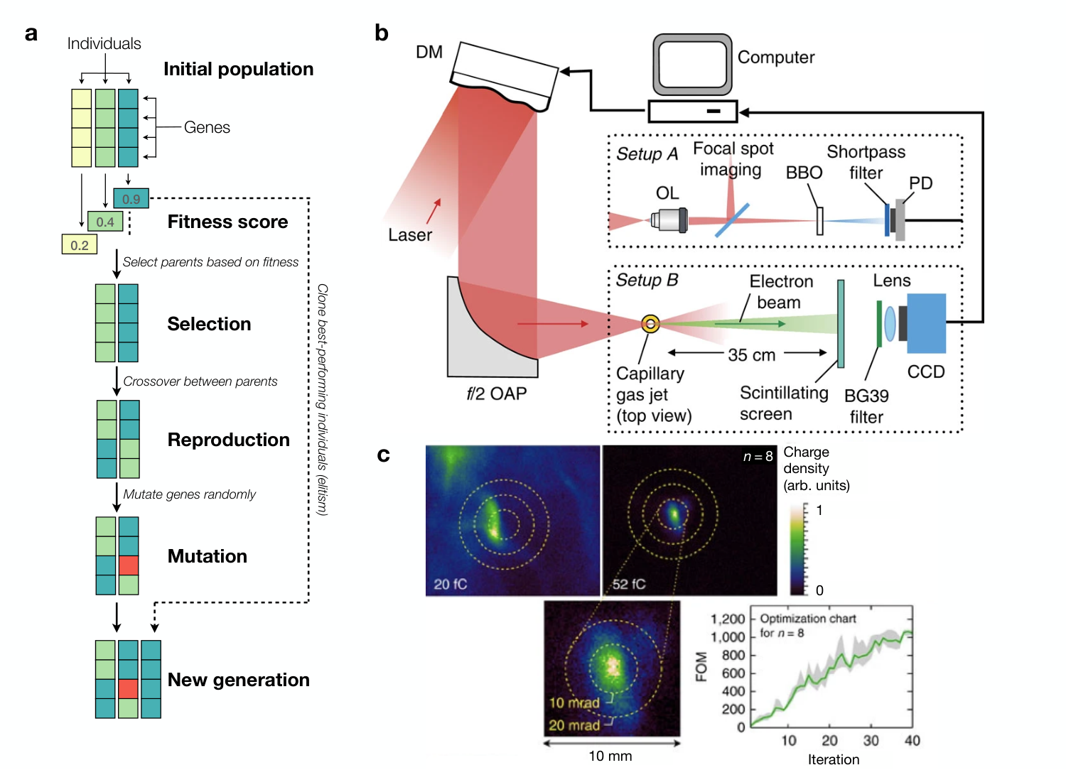
IV.2 Grid search and random search
Once an objective is defined, we can try to optimize it. One of the simplest methods to do so is a grid search, where the input parameter space is explored by taking measurements in regularly-spaced intervals. This technique is particularly simple to implement, especially in experiments, and therefore remains very popular in the setting of experimental laser physics. However, the method severely suffers from the ”curse of dimensionality”, meaning that the number of measurements increases exponentially with the number of dimensions considered. In practice, the parameter space therefore has to be low-dimensional (one-, two- or three-dimensional at most) and it is applied to the optimization of selected parameters that appear to influence the outcome the most. One issue with grid scans is that they can lead to aliasing, i.e. high-frequency information can be missed due to the discrete grid with a fixed sampling frequency.
A popular variation, in particular in laser-plasma experiments, is the use of sequential 1-D line searches. Here, one identifies the optimum in one dimension, then performs a scan of another parameter and moves to its optimum, and so forth. This method can converge much faster to an optimum, but is only applicable in settings with a single, global optimum.
Random search is a related method where the sampling of the input parameter space is random instead of regular. This method can be more efficient than grid search, especially if the system involves coupled parameters and has a lower effective dimensionality 209. It is therefore often used in optimization problems with a large number of free parameters. However, purely random sampling also has drawbacks. For instance, it has a tendency to cluster, i.e. to sample points very close to another while leaving some areas unexplored. This behavior is undesirable for signals without high-frequency components and instead one would rather opt for a sampling that explores more of the parameter space. For this case, a variety of schemes exist that combine features of grid search and random search. Two popular examples are jittered sampling and Latin hypercube sampling 210. For the former samples are randomly placed within regularly-spaced intervals, while the latter does so while maintaining an even distribution in the parameter space.
Grid and random search are often used for initial exploration of a parameter space to seed subsequent optimization with more advanced algorithms. An example for this is shown in Fig. 15a, where grid search is combined with the downhill simplex method discussed in the next section.
IV.3 Downhill simplex method and gradient-based algorithms
In the downhill simplex method, also known as Nelder-Mead algorithm211, an array of input parameter sets from an -dimensional space is evaluated to get the corresponding function values. The worst-performing evaluation point is modified at each iteration by translating it towards or through the center of the simplex. This continues until the simplex converges to a point at which the function is optimized. The method is simple and efficient, which is why it is popular in various optimization settings. The convergence speed crucially depends on the initial choice of the simplex, with a large distance between input parameters leading to a more global optimization, while small simplex settings result in local optimization.
In the limit of small simplex size, the Nelder-Mead algorithm is conceptually related to gradient-based methods for optimization. The latter are based on the concept of using the gradient of the objective function to find the direction of the steepest slope. The objective function is then minimized along this direction using a suitable algorithm such as gradient descent. Momentum descent is a popular variation of gradient descent where the gradient of the function is multiplied by a value, in analogy to physics called momentum, before being subtracted from the current position. This can help the algorithm converge to the local minimum faster. These methods typically require more and smaller iterations than the downhill simplex method, but can be more accurate.
In both cases, measurement noise can easily result in a wrong estimation of the gradient. In the setting of laser-plasma experiments, it is therefore important to reduce such noise, e.g. by taking several measurements at the same position. While this may be possible when working with high-repetition-rate systems, as was demonstrated by Dann et al. 201, gradient-based methods are in general less suitable to be used in high-power-laser settings. Other popular derivative-based algorithms are the conjugate gradient (CG) methods, quasi-Newton (QN) methods, and the limited-memory Broyden-Fletcher-Goldfarb-Shanno (L-BFGS) method, all of which are discussed by Nocedal and Whright154.
IV.4 Genetic algorithms
One of the first family of algorithms to find applications in the field laser-plasma acceleration was genetic algorithm. As a subclass of evolutionary methods, these nature-inspired algorithms start with a pre-defined or random set, called population, of measurements for different input settings. Each free parameter is called a gene and, similar to natural evolution, these genes can either cross over between most successful settings or randomly change (mutate). This process is guided by a so-called fitness function, which is designed to yield a single-valued figure of merit that is aligned with the optimization goal. Depending on the objective, the individual measurements are ranked from most to least fit. The fittest “individuals” are then used to spawn a new generation of “children”, i.e. a new set of measurements based on crossover and mutation of the parent genes. A popular variation to genetic algorithms is differential evolution212, which employs a different type of crossover. Instead of crossing over two parents to create a child, differential evolution uses three parent measurements. The child is then created by adding a weighted difference between the parents to a random parent. This process is repeated until a new generation is created, see Fig. 15b for an example.
One particular strength of genetic algorithms compared to many other optimization methods is their ability to perform multi-objective optimization, i.e. when multiple, potentially conflicting, objectives are to be optimized. A popular example would be the nondominated sorting genetic algorithms (NSGAs)213. Here the name-giving sorting technique ranks the individuals by their population dominance, i.e. how many other individuals in the population the individual dominates. Other multi-objective approaches are for instance based on optimizing niches, similar-valued regions of the Pareto front214.
It should be noted that genetic algorithms intrinsically operate on population batches and not on a single individual. While this can be beneficial for parallel processing in simulations, it can make it more difficult to employ in an online optimization setup.
IV.5 Bayesian optimization
Bayesian optimization (BO)230, 231 is a model-based global optimization method that uses probabilistic modeling, which was discussed in Section II.1.3. The strength of BO lies in its efficiency with regard to the number of evaluations. This is particularly useful for problems with comparably high evaluation costs or long evaluation times. To achieve this, BO uses the probabilistic surrogate model to make predictions about the behavior of the system at new input parameter settings, providing both a value estimate and an uncertainty.
At the core of BO lies what is called the acquisition function; a pre-defined function that is suggest the next points to probe on a probabilistic model. The latter is usually99 9 While most work on BO is done using GP regression, the method is in principle model agnostic. This means that other types of (probabilistic) surrogate models of the system can be employed, such as decision trees (see Section II.1.5) or deep neural networks (see Section II.1.6). a Gaussian process fitted from training points, see Section II.1.4, thus providing a cheap-to-evaluate surrogate function. A simple and intuitive example of an acquisition function is the upper confidence bound,
| (27) |
which weighs the mean prediction versus the variance prediction , with a user-chosen hyperparameter . For the optimization will act entirely exploitatively, i.e. it will move to the position of the highest expected return, whereas a large incentivises to reduce the uncertainty and explore the parameter space. Other common acquisition functions are the expected improvement 233, knowledge gradient234 and entropy search235. As the surrogate model can be probed at near-negligible evaluation cost, this optimization can be performed using numerical optimization methods such as the gradient-based methods discussed in Section IV.3. The position of the acquisition function’s optimum is then used as input parameter setting to evaluate the actual system. This process is repeated until some convergence criteria is achieved, a predefined number of iterations are reached, or the allocated resources have been otherwise exhausted.
Bayesian optimization provides a very flexible framework that can be further adapted to various different optimization settings. For instance, it has proven to be a valid alternative to evolutionary methods when it comes to solving multi-objective optimization problems. The importance of this method for laser-plasma acceleration stems from the fact that many optimization goals, such as beam energy and beam charge, are conflicting in nature and require a definition of a trade-off. The goal of the Pareto-optimization is to find the Pareto-front, which is a surface in the output objective space that is comprised of all the non-dominated solutions (see Section IV.1.2). A common metric that is used to measure the closeness of a set of points to the Pareto-optimal points is the hypervolume. The BO algorithm works by using the expected hypervolume improvement236 to increase the extent of the current non-dominated solutions, thus optimizing all possible combinations of individual objectives. Note that the Pareto-front, like to the global optimum of single-objective optimization, is usually not known a priori.
Another possible way to extend BO is to incorporate different information sources237. This is often done by adding an additional information input dimension to the data model. This method is often referred to as multi-task (MT) or multi-fidelity (MF) BO. Both terms being used somewhat interchangeably in the literature, although MT often refers to optimization with entirely different systems (codes, etc.), whereas MF focuses on different fidelity (resolution, etc.) of the same information source. The core concept behind these methods is that the acquisition function not only encodes the objective, but also minimizes the measurement cost. These multi-information-source methods have the potential to speed up optimization significantly. They can also be combined with multi-objective optimization, as shown by Irshad et al.206.


IV.6 Reinforcement learning
Reinforcement learning (RL)242 differs fundamentally from the optimization methods discussed so far. RL is a method of learning the optimal behavior (the policy ) to control a system. The learning occurs via repeated trial and error, called episodes, where each episode is started in an initial state of the system, and then the agent (i.e., the optimizer) interacts with the system according to its policy. The agent then receives a reward signal, which is a scalar value that indicates the success of the current episode and its goal is to maximize the expected reward, analogous to the objective function in other optimization methods. The agent is said to learn when it is able to improve its policy to achieve a higher expected reward.
The policy itself has traditionally been represented using a Markov decision process (MDP), but in recent years deep reinforcement learning (DRL) has become widely used, in which the policy is represented using deep neural networks243, 244. However, while we commonly update weights and biases via backpropagation in supervised deep learning, the learning in DRL is done in an unsupervised way. Indeed, while the agent is trying to learn the optimal policy to maximize the reward signal, the reward signal itself is unknown to the agent. The agent only knows the reward signal at the end of the episode, so it is not possible to perform backpropagation. Instead, the policy network can for instance be updated using evolutionary strategies (see Section IV.4), where the agents achieving the highest reward are selected to create a new generation of agents. Another common approach is to use a so-called actor-critic strategy245, where a second network is introduced, called the critic. At the end of each episode, the critic is trained to estimate the expected long-term reward from the current state, called the value. This expected reward signal is then used to train the actor network to adjust the policy. The policy gradient246 is a widely used algorithm for training the policy network using the critic network to calculate the expected reward signal.
Reinforcement learning algorithms can be further divided into two main classes: model-free and model-based learning. Model-free methods learn as discussed above directly by trial and error, only implicitly learning about the environment. Model-based methods, on the other hand, explicitly build a model of the environment, which can be used for both planning and learning (somewhat similar to optimization using surrogate models discussed earlier). The arguably most popular method to build models in reinforcement learning is again the use of neural networks, as they can learn complex, non-linear relationships and are also capable of learning from streaming data, which is essential in reinforcement learning. A crucial advantage of the model-based approach is that it can drastically speed up training, although performance is always limited by the quality of the model. In the case of real-life systems this is sometimes referred to as the ‘reality gap’.
One crucial advantage of reinforcement learning is that once the training process is completed, the computational requirements of running an optimization are heavily reduced. A simplified representation of the reinforcement learning workflow is sketched in Fig. 16.
V Unsupervised Learning
In this section we are going to discuss unsupervised learning techniques for exploratory data analysis. The term ‘unsupervised’ refers to the case where one does not have access to training labels, and therefore the aim is not to find a mapping between training data and labels, as it is often the case for deep learning. Rather, the aim is to detect relationships between features of the data.
For high-power laser experiments, many parameters will be coupled in some way such that there are correlations between different measurable input quantities. For example, increasing the laser energy in the amplifier chain of a high-power laser can affect the laser spectrum or beam profile. To understand the effect a change to any one of these parameters will have, it is important to consider their correlation. However, an experimental setup can easily involve tens of parameters and interpreting correlations becomes increasingly difficult. In this context, it can be useful to distill the most important (combinations of) parameters in a process called dimensionality reduction. The same method also plays a crucial role in efficient data compression, which is becoming increasingly important due to the large amount of data produced in both experiments and simulation. These methods are also closely related to Pattern Recognition, which addresses the issue of automatically discovering patterns in data.
V.1 Clustering
Data clustering is a machine learning task of finding similar data points and dividing them into groups, even if the data points are not labeled. This can for instance be useful to separate signal from background in physics experiments.
A popular centroid-based clustering algorithm is the -means algorithm, which consists of two steps: First, the algorithm randomly assigns a cluster label to each point. Then, in a second step, it calculates the center point of each cluster and re-assigns the cluster label to each point based on the proximity to the cluster center. This process is repeated until the cluster assignment does not change anymore. The in the algorithm’s name represents the number of clusters, which can be guessed or - more quantitatively - be estimated using methods such as the ”silhouette” value or the ”elbow method” 252. As the method is quite sensitive to the initial random choice of the cluster assignment, it is often run several times with different initial choices to find the optimal classification.
In contrast to centroid-based clustering, in which each cluster is defined by a center point, in distribution-based clustering, each cluster is defined by a (multivariate) probability distribution. In the simplest case this can be a Gaussian distribution with a certain mean and variance for each cluster. More advanced methods use a Gaussian mixture model (GMM), in which each cluster is represented as a combination of Gaussian distributions. A popular distribution-based clustering method is the expectation maximization (EM) algorithm 158.

V.2 Correlation analysis
A simple method for exploring correlations is the correlation matrix, which is a type of matrix that is used to measure the relationship between two or more variables. We can calculate its coefficients, also known as Pearson correlation coefficients, on a set of measurements of each pair of parameters and as
| (28) |
where and are the mean values of the variables and , respectively. The correlation coefficient is a number between -1 and 1. A value of 1 means that two variables are perfectly correlated, while a value of -1 means that two variables are perfectly anti-correlated. A value of 0 means that there is no correlation between two variables.
The correlation matrix and its visualization, sometimes called correlogram, allow for a quick way to look for interesting and unexpected correlations. An example for this is shown in Fig. 18. Note that by reducing correlations to a single linear term one can miss more subtle or complex relationships between variables. For such cases more general measures of correlation exist, such as the Spearman correlation coefficient that measures how well two variables can be described by any monotonic function.

V.3 Dimensionality reduction
Many data sets are high-dimensional data but are governed by few important underlying parameters. Signal decomposition and dimensionality reduction are processes that reduce the dimensionality of the data by separating a signal into its components or projecting it onto a lower-dimensional subspace so that the essential structure of the data is preserved. There are many ways to perform dimensionality reduction, two of the most common ones being principal component analysis and autoencoders.
Principal component analysis (PCA) is a very popular linear transformation technique that is used to convert a set of observations of possibly correlated variables into a (smaller) set of values of linearly uncorrelated variables, called the principal components. This transformation is defined in such a way that the first principal component has the largest possible variance, and each succeeding component in turn has the highest variance possible under the constraint that it is orthogonal to the preceding components. One method to perform PCA is to use singular value decomposition (SVD), which is used to decompose the matrix of data into a set of eigenvectors and eigenvalues. PCA shares a close relationship with correlation analysis, as the eigenvectors of the correlation matrix match those of the covariance matrix, which is utilized in defining PCA. Additionally, the eigenvalues of the correlation matrix equate to the squared eigenvalues of the covariance matrix, provided that the data has been normalized. Kernel PCA254 is an extension of PCA that uses a nonlinear transformation of the data to obtain the principal components. A relatively new variation, with some relation to the priorly discussed compressed sensing (Section III.4), is robust principal component analysis (RPCA)255. RPCA is a modification of the original algorithm, which is better suitable to handle the presence of outliers in data sets. PCA should not be confused with the similarly named independent component analysis (ICA)256, which is a popular technique to decompose a multivariate signal into a sum of statistically independent non-Gaussian signals.
There are also many neural network approaches to dimensionality reduction, one of the most popular ones being autoencoders (AEs). The purpose of an AE is to learn an approximation to the identity function, i.e. a function that reproduces the input. In a standard AE, a neutral network is created with an intermediate bottleneck layer with a reduced number of nodes, known as the latent space. During training, the neural network hyperparameters are optimized so that the output matches the input as closely as possible, typically by minimizing the mean-squared error. Due to the bottleneck, the autoencoder automatically discovers an efficient representation for the data in the latent space. The hidden layers up to the latent space are known as the decoder and the the hidden layers from the latent space to the output layer are the encoder. The encoder can then be used separately to perform dimension reduction, equivalent to lossy data compression. With the corresponding decoder, an approximation of the original data can be extracted from its latent space.
There exist many different types of autoencoder architecture, a particularly popular one being variational autoencoders (VAEs). VAEs replace deterministic encoder-decoder layers with a stochastic architecture (c.f. Fig. 6) to allow the model to provide a probability distribution over the latent space. As a result, a VAEs latent space is smooth and continuous in contrast to a standard AEs latent space, which is discrete. This allows VAEs to also generate new data by sampling from the latent space.
Autoencoders have also shown a strong potential as advanced compression techniques that can be highly adapted to many kinds of inputs. In this case, one trains an AE model to find an approximation of the identity function for some raw data. After training, the raw data is sent through the encoding layer and only the dimensionality-reduced, highly-compressed latent space representation in the bottleneck layer is saved. Decompression is achieved by sending the data through the decoding layer. This method is not only relevant to reduce disc space occupied by data. Autoencoders are nowadays frequently used as an integral part of complex machine learning tasks, where the latent space is used a lower-dimensional input for e.g. a diffusion network (as part of what is called a latent diffusion model257) or a Bayesian optimizer258.
VI Image analysis

In the previous section we have discussed how to analyze datasets by looking for correlations or compressed representations. A closely related group of tasks occurs when dealing with image data, i.e. image recognition or classification, object detection and segmentation. While the methods in the previous section dealt with features learnt from the data itself, the techniques discussed in this section aim to identify or locate specific features in our data (in particular images). As such, these are all considered supervised learning methods.
VI.1 Classification
The classification problem in machine learning is the problem of correctly labeling a data point from a given set of data points with the correct label. The data points are labeled with a categorical class label, such as “cat”, “dog”, “electron” or “ion”, see Fig. 19a.
In the following we are going to briefly discuss some of the most important machine-learning techniques used for classification. It should be noted that classification is closely related to regression, with the main difference being essentially that the model’s output is a class value instead of a value prediction. As such, methods working in regression can in general also be applied to classification tasks. One example is the decision tree method, which we already discussed in Section II.1.5.
VI.1.1 Support vector machines
Support vector machines (SVMs) are a popular set of machine learning methods used primarily in classification and recognition. For a simple binary classification task, an SVM draws a hyperplane that divides all data points of one category from all data points of the other category. While there could be many hyperplanes, an SVM looks for the optimal hyperplane that best separates the dataset by maximizing the margin between the hyperplane and the data points in both categories. The points that locate right on the margin are called “supporting vectors”. For a dataset with more than two categories, classification is performed by dividing the multi-classification problem into several binary classification problems and then finding a hyperplane for each. In practice, the data points in two categories can mix together so that they can not be clearly divided by a linear hyperplane. For such nonlinear classification tasks, the kernel trick is used to compute the nonlinear features of the data points and map them to a high dimensional space, so that a hyperplane can be found to separate the high dimensional space. The hyperplane will then be mapped back to the original space.
The ideal application scenario for an SVM is for datasets with small samples but high dimensions. The choice of various kernel functions also adds to the flexibility of this method. However, an SVM would be very computationally expensive for large datasets. Besides, its accuracy can significantly decrease when analyzing datasets with large noise level as the hyperplanes can not be defined precisely. Therefore, especially in the context of high-power laser experiments, one has to be cautious to apply SVMs if there are considerable stability issues.
VI.1.2 Convolutional neural networks
Convolutional neural networks (CNNs) are a type of neural network (cf. Section II.1.6) that is particularly well-suited for image classification261, but are also used in various other problems.
Such a network is composed of sequential convolutional layers, in each of which, an kernel (or “filter” matrix) is convolved with the output of the previous layer. This operation is done by sliding the kernel over the input image, and each pixel in the output layer is calculated by the dot product of the kernel with a sub-section of the input image centered around the corresponding pixel. Resultingly, convolutional layers are capable of detecting local patterns in the region of the kernel. The kernel is parameterised with weights, which are learned via backpropagation as in a regular neural network. Within a layer, there can also be multiple channels of the output; practically thought of as multiple kernels being passed over the image, allowing for different features to be detected. The early layers of a CNN detect simple structures such as edges, but by adding multiple layers with varying kernel sizes, the network can perform high level abstraction in order to detect complicated patterns.
The convolutional layer makes the CNN very efficient for image classification. It allows the network to learn translation-invariant features - a feature learned at a certain position of an image can be recognized at any position on the same image.
In order to detect patterns that are non-local in the image, pooling is often applied. There exist many schemes of pooling, but the general concept is to take a set of pixels in the input and to apply some operation that turns them into 1 pixel. Examples include max-pooling (taking the maximum of the set of pixels) and average pooling. This operation decreases the dimensions of the image, and therefore allows a subsequent convolutional layer with the same kernel to detect features that were much further apart in the original image. Typical CNNs will use multiple pooling layers to decrease the dimensions until a kernel can nearly span the whole image to detect any non-local pattern. The output is then flattened and several fully connected layers can be used to manipulate the data for the relevant (ie. regression or classification) task.
While the use of deeper CNNs with an increasing number of layers tends to improve performance262, architectures can suffer from unstable gradients in training via backpropagation263, showing that some deeper architectures are not as easy to optimize. One particularly influential solution to this problem was the introduction of the residual shortcut, where the input to a block is added to the output of the block. In backpropagation, this enables the ‘skipping’ of layers, effectively simplifying the network and leading to better convergence. This was first proposed and implemented in ResNet 264, which has since become a standard for deep CNN architectures265, with any number of variations. It should be mentioned though that a number of competitive networks without residual shortcuts exist, e.g. AlexNet 266.

VI.2 Object detection
In the context of image data, object detection can be seen as an extension of classification, yielding both a label as in classification tasks and the position of that object, illustrated in Fig. 19b. The main challenge is that complex images can contain many objects with different features, while the number of objects can also differ from one image to another. Therefore, object detection techniques require a certain flexibility regarding their structure.
The Viola-Jones algorithm268 is one of the most popular object detection algorithms from the 2000s, pre-dating the recent network-based object detectors. Generally, it involves detecting objects by looking at the image as a set of small patches, and identifying so-called Haar-like features. The latter are patterns that occur frequently in images, and can be used to distinguish between different objects. Viola-Jones detects objects by first analyzing an image at different scales. For each scale, it looks for features by scanning the image with a sliding window, and for each window, it computes a list of features used to identify the object. If the object is detected, the algorithm returns the bounding box of the object. The Viola-Jones framework does not allow for simultaneous classification and instead requires a subsequent classifier such as an SVM for that task. Compared to its network-based alternatives, Viola-Jones is worse in terms of precision but better in terms of computational cost, allowing real-time detection at high frame rates269.
Object detection networks are more complicated than a regular CNN, because the length of the output layer of the neural network can not be pre-defined due to the unknown number of objects on an image. A possible solution is to divide the image into many regions and to construct a CNN for each region, but that leads to significant computational cost. Two family of networks are developed to detect objects at reasonable computational cost. The region proposal network (RPN) takes an image as input and outputs a set of proposals for possible objects in the image. A CNN is used to find features in each possible region and to classify the feature into known category. The RPN is trained to maximize the overlap between the proposals and the ground truth objects. The state-of-the-art algorithm in this family is the Faster-RCNN270.
An alternative to region-based CNNs is the YOLO271 family. YOLO stands for “You Only Look Once” as it only looks at the image once with a single neural network to make predictions. This is different from other object detection algorithms, which often employ many neural networks for the image. As a result, YOLO is typically much faster, allowing for real-time object detection. The disadvantage is that it is not as accurate as some of the other object detection algorithms. Nevertheless, the fast inference speed of YOLO is particularly appealing to high-power laser facilities with high-repetition-rate capability.
VI.3 Segmentation
Semantic segmentation272 is a related task in computer vision that seeks to create a pixel-by-pixel mapping of the input image to a class label, not only a bounding box as in object detection, see Fig. 19c. By doing so, segmentation defines the exact boundary of the objects.
Many semantic segmentation architectures are based on a fully convolutional networks (FCNs) 273 and have evolved considerably in recent years. Since FCNs suffered from the issue of semantic gaps, where the output had a much lower resolution than the input, skip connections were introduced to allow the gradient to backpropagate through the layers to improve the performance. An example of such advanced network architectures is the U-Net 186 and the DeepLab network 272, which is based on ResNet-101. Both of these architectures use residual skip connections to maintain gradient flow. The advantage of semantic segmentation compared to standard object detection is that the network can easily localize multiple objects of the same class in an image. The disadvantage is that one needs to train a separate network for each class.
Related is instance segmentation274, which goes a step further and distinguishes each individual instance of an object, not just the class. Instance segmentation is a significant challenge, as it requires the network to be able to distinguish between two instances of the same object, e.g. two cats. Instance segmentation architectures are typically based on Mask R-CNN275, which combines a CNN with a region-based convolutional neural network (R-CNN)276 and a fully convolutional network (FCN)273. Note that mask R-CNN can be used for both semantic and instance segmentation.
| Author, Year | Problem Type | ML Technique | Sim. | Exp. | Research field |
|---|---|---|---|---|---|
| Humbird et al., 2018 96 | Forward model | Neural net decision tree | ✓ | ✗ | Inertial confinement fusion |
| Humbird et al., 2018 97 | Forward model | Transfer learning | ✓ | ✓ | Inertial confinement fusion |
| Gonoskov et al., 2019108 | Forward model | Neural Network | ✓ | ✓ | High-harmonic generation |
| Maier et al., 2020 26 | Forward model | Linear Regression | ✓ | ✗ | Laser wakefield acceleration |
| Kluth et al., 2020 99 | Forward model | Autoencoder DJINN | ✓ | ✓ | Inertial confinement fusion |
| Kirchen et al., 2021 29 | Forward model | Neural Network | ✗ | ✓ | Laser wakefield acceleration |
| Rodimkov et al., 2021109 | Forward model | Neural Network | ✓ | ✗ | Noise robustness in PIC codes |
| Djordjevic et al., 2021 110 | Forward model | Neural Network | ✓ | ✗ | Laser-ion acceleration |
| Watt et al., 2021 111 | Forward model | Neural Network | ✓ | ✗ | Strong-field QED |
| McClarren et al., 2021 112 | Forward model | Neural Network | ✓ | ✗ | Inertial confinement fusion |
| Simpson et al., 2021 113 | Forward model | Neural Network | ✗ | ✓ | Laser-solid interaction |
| Streeter et al., 2023 114 | Forward model | Neural Network | ✗ | ✓ | Laser wakefield acceleration |
| Krumbügel et al., 1996 | Inverse problem | Neural network | ✗ | ✓ | Spectral Phase Retrieval |
| Sidky et al., 2005282 | Inverse problem | EM algorithm | ✗ | ✓ | X-ray spectrum reconstruction |
| Döpp et al., 2018168 | Inverse problem | Statistical iterative reconstruction | ✗ | ✓ | X-ray tomography with betatron radiation |
| Huang et al., 2014177 | Inverse problem | Compressed sensing | ✓ | ✗ | ICF radiation analysis |
| Zahavy et al., 2018193 | Inverse problem | Neural network | ✗ | ✓ | Spectral Phase Retrieval |
| Hu et al., 2020194 | Inverse problem | Neural network | ✗ | ✓ | Wavefront measurement |
| Ma et al., 2020179 | Inverse problem | Compressed sensing | ✗ | ✓ | Compton X-ray tomography |
| Li et al., 2021283 | Inverse problem | Compressed sensing | ✓ | ✗ | ICF radiation analysis |
| Howard et al., 2023 | Inverse problem | Compressed sensing / Deep unrolling | ✓ | ✗ | Hyperspectral phase imaging |
| Bartels et al., 2000215 | Optimization | Genetic algorithm | ✗ | ✓ | High-harmonic generation |
| Yoshitomi et al., 2004216 | Optimization | Genetic algorithm | ✗ | ✓ | High-harmonic generation |
| Zamith et al., 2004218 | Optimization | Genetic algorithm | ✗ | ✓ | Cluster dynamics |
| Yoshitomi et al., 2004217 | Optimization | Genetic algorithm | ✗ | ✓ | Cluster dynamics |
| Nayuki et al., 2005219 | Optimization | Genetic algorithm | ✗ | ✓ | Ion acceleration |
| He et al., 2015200, 220 | Optimization | Genetic algorithm | ✗ | ✓ | Laser wakefield acceleration |
| Streeter et al., 2018227 | Optimization | Genetic algorithm | ✗ | ✓ | Cluster dynamics |
| Lin et al., 2019221 | Optimization | Genetic algorithm | ✗ | ✓ | Laser wakefield acceleration |
| Dann et al., 2019201 | Optimization | Genetic & Nelder-Mead algorithms | ✗ | ✓ | Laser wakefield acceleration |
| Shalloo et al., 2020202 | Optimization | Bayesian optimization | ✗ | ✓ | LWFA, betatron radiation |
| Smith et al., 2020229 | Optimization | Genetic algorithm | ✓ | ✗ | Laser-ion acceleration |
| Kain et al., 2020247 | Optimization | Reinforcement learning | ✓ | ✓ | Plasma wakefield acceleration |
| Jalas et al., 2021203 | Optimization | Bayesian optimization | ✓ | ✓ | Laser wakefield acceleration |
| Pousa et al., 2022241 | Optimization | Bayesian optimization | ✓ | ✗ | Laser wakefield acceleration |
| Dolier et al., 2022239 | Optimization | Bayesian optimization | ✓ | ✗ | Laser-ion acceleration |
| Irshad et al., 2023205, 253 | Optimization | Bayesian optimization | ✓ | ✓ | Laser wakefield acceleration |
| Loughran et al., 2023240 | Optimization | Bayesian optimization | ✗ | ✓ | Laser-ion acceleration |
| Chu et al., 2019 279 | Image Analysis | Neural Network | ✗ | ✓ | Laser damage segmentation |
| Amorin et al., 2019 277 | Image Analysis | Neural Network | ✗ | ✓ | Laser damage analysis |
| Li et al., 2020 281 | Image Analysis | Neural Network | ✗ | ✓ | Laser damage detection in 3D |
| Hsu et al., 202098 | Feature analysis | Six supervised learning methods | ✗ | ✓ | Inertial confinement fusion |
| Lin et al., 2021100 | Feature analysis | Four supervised learning methods | ✗ | ✓ | Laser wakefield acceleration |
| Willmann et al., 2021259 | Dimensionality reduction | Autoencoder | ✓ | ✗ | Laser wakefield acceleration |
| Stiller et al., 2022260 | Data compression | Autoencoder | ✓ | ✗ | Laser wakefield acceleration |
| Pascu, 2022 278 | Image Analysis | SVM / Neural Network | ✗ | ✓ | Laser anomaly detection |
| Soltane et al., 2022280 | Image Analysis | Neural Network | ✗ | ✓ | Laser damage segmentation |
| Lin et al., 2023 267 | Image Analysis | Neural Network | ✗ | ✓ | Laser wakefield acceleration and damage detection |
VII Discussion and Conclusions
In this paper, we have presented an overview of techniques and recent developments in machine learning for laser-plasma physics. As we have seen, early proof-of-concept papers appeared in the late 1990s and early 2000s, but the computing power available at the time was typically not sufficient to make the approaches competitive with established methods or to reach a suitable level of accuracy. In the mid-2010s, a resurgence of interest in the field began, with an ever-increasing number of publications. A significant fraction of the papers that have been reviewed here are experimental in nature, especially regarding optimization, see Table 2. On one hand, this can be attributed to the increasing digitization of the laboratory environment, with control systems, data acquisition, and other developments providing access to large amounts of data. On the other hand, the complexity of modern experiments acts as a catalyst for the development of automated data analysis and optimization techniques. Deployment of machine-learning techniques in a real-world environment can however be challenging, e.g. due to noise, jitter and drifts. This is certainly one of the reasons why the most advanced machine learning techniques, such as multi-objective optimization or deep compressed sensing, tend to be first tested with simulations.
Among the methods being employed we also observed some general trends. For instance, while genetic algorithms have been very popular in the past for global optimization, there has been an increasing amount of papers focusing on Bayesian optimization. This is likely due to the fact that both simulations and experiments in the context of laser-plasma physics are very costly, making the use of Bayesian approaches more appealing. In most experimental settings, local optimization algorithms such as gradient descent or the Nelder-Mead algorithm are less suitable because of the large number of iterations needed and their sensitivity to noise. Reinforcement learning, especially in its model-free incarnation, suffers from the same issue, which explains why only very few examples of its use exist in adjacent research fields. While rather popular among data scientists due to their simplicity and interpretability, decision tree methods have not seen wide application in laser-plasma physics. In part, this is likely due to the fact that these methods are often considered to have more limited capabilities in comparison to neural networks, making it more attractive to directly use deep neural networks. In the context of ill-posed inverse problems it is to be expected that end-to-end neural networks or hybrid approaches will gradually replace traditional methods, such as regularization via total variation. That said, the simplicity and bias-free nature of least-squares methods are likely to ensure their continued popularity, at least in the context of easier to solve well-posed problems.
Much of the success of machine-learning techniques stems from the fact that they are able to leverage prior knowledge, be it in the form of physical laws (e.g. via physics-informed neural networks) or in the form of training data (e.g. via deep learning). Regarding the latter, the importance of preparing input data cannot be overstated. A popular saying in supervised learning is ”garbage in, garbage out”, meaning that the quality of a model’s output heavily depends on the quality of the training data. Important steps are for instance pre-processing284 (noise removal, normalization, etc.) and data augmentation285 (rotation, shifts, etc.). The latter is of particular importance when dealing with experimental data, for which data acquisition is usually costly, making it challenging to acquire enough data to train a well-performing model. Furthermore, even when using regularization techniques, diversity of training data is very important to ensure good generalization capabilities and to avoid bias.
Two outstanding issues for a wide adoption of machine learning models in the laser-plasma community are interpretability and trustworthiness, both regarding the model itself and on the user side. While some machine-learning models such as decision trees can be interpreted comparably easily, the inner workings of advanced models like deep neural networks are often difficult to understand. This issue is amplified by the fact that integrated machine learning environments allow users to quickly build complex models without a thorough understanding of the underlying principles. We hope that this review will help to alleviate this issue, by providing a better understanding of the origin, capabilities and limitations of different machine-learning techniques. Regarding trustworthiness, quantification of aleatoric uncertainty in training data and epistemic uncertainty of the model remains an important research area286. For instance, well-tested models may break down when exposed to unexpected input data, e.g. due to drifts in experimental conditions or changes in the experimental setup. Such issues can for instance be addressed by incorporating uncertainty quantification into models to highlight unreliable predictions.
As our discussion has shown, there is an ever increasing interest in data-driven and machine learning techniques within the community and we hope that our paper provides useful guidance for those starting to work in this rapidly evolving field. To facilitate some hands-on experimentation, we conclude with a short guide how to get started to implement the techniques we discussed in this paper. Most of these are readily implemented in several extensive libraries: Scikit-learn287, Tensorflow288, and PyTorch289 being among the most popular ones. Each of these libraries has its own strengths and weaknesses. In particular, deep learning libraries such as Tensorflow and PyTorch are tailored for fast computations on graphics processing units (GPUs), whereas libraries such as Scikit-learn are designed for more general machine learning tasks. Higher level frameworks exist to facilitate the training of neural networks, e.g. MLflow or PyTorch lightning.
The Darts library290 contains implementations of various time series forecasting models, and also acts as a wrapper for numerous other libraries related to forecasting. Many numerical optimization algorithms such as derivative-based methods and differential evolution can be easily explored using the optimization library of SciPy291. While this includes for instance differential evolution, more sophisticated evolutionary algorithms such as multi-objective evolutionary methods require dedicated libraries like pymoo292 or PyGMO293. Bayesian optimization can for instance be implemented within Scikit-learn or using the experimentation platform Ax. The highly-optimized BoTorch library294 can be used for more advanced applications, including for instance multi-objective, multi-fidelity optimization. Some libraries are specifically tailored to hyperparameter optimization, such as the popular optuna library295.
While all of the above examples are focused on python as an underlying programming language, machine learning tasks can also be performed using many other programming platforms or languages such as Matlab or Julia. Jupyter notebooks provide a good starting point and some online implementations, such as Google Colab, even give limited access to GPUs for training. The reader is encouraged to explore the various frameworks and libraries to find the one that best suits their needs.
Acknowledgements
We thank all participants of the LPA Online Workshop on Control Systems and Machine Learning for their contributions to the workshop, many of which are referenced throughout this manuscript. We particularly thank N. Hoffmann, S. Jalas, M. Kirchen, R. Shalloo and A.G.R. Thomas for helpful feedback and comments on the manuscript. The authors acknowledge the use of GPT-3296 (text-davinci-003) in the copy-editing process of this manuscript.
References
- [1] Colin Danson, David Hillier, Nicholas Hopps, and David Neely. Petawatt class lasers worldwide. High Power Laser Science and Engineering, 3:e3, 2015.
- [2] Colin N. Danson, Constantin Haefner, Jake Bromage, Thomas Butcher, Jean-Christophe F. Chanteloup, Enam A. Chowdhury, Almantas Galvanauskas, Leonida A. Gizzi, Joachim Hein, David I. Hillier, Nicholas W. Hopps, Yoshiaki Kato, Efim A. Khazanov, Ryosuke Kodama, Georg Korn, Ruxin Li, Yutong Li, Jens Limpert, Jingui Ma, Chang Hee Nam, David Neely, Dimitrios Papadopoulos, Rory R. Penman, Liejia Qian, Jorge J. Rocca, Andrey A. Shaykin, Craig W. Siders, Christopher Spindloe, Sándor Szatmári, Raoul M. G. M. Trines, Jianqiang Zhu, Ping Zhu, and Jonathan D. Zuegel. Petawatt and exawatt class lasers worldwide. High Power Laser Science and Engineering, 7:e54, 2019.
- [3] Alexander Pukhov. Strong field interaction of laser radiation. Reports on Progress in Physics, 66(1):47, 2003.
- [4] Mattias Marklund and Padma K. Shukla. Nonlinear collective effects in photon-photon and photon-plasma interactions. Reviews of Modern Physics, 78(2):591–640, 2006.
- [5] J. M. Cole, K. T. Behm, E. Gerstmayr, T. G. Blackburn, J. C. Wood, C. D. Baird, M. J. Duff, C. Harvey, A. Ilderton, A. S. Joglekar, K. Krushelnick, S. Kuschel, M. Marklund, P. McKenna, C. D. Murphy, K. Poder, C. P. Ridgers, G. M. Samarin, G. Sarri, D. R. Symes, A. G. R. Thomas, J. Warwick, M. Zepf, Z. Najmudin, and S. P. D. Mangles. Experimental Evidence of Radiation Reaction in the Collision of a High-Intensity Laser Pulse with a Laser-Wakefield Accelerated Electron Beam. Physical Review X, 8(1):011020, 2018.
- [6] K. Poder, M. Tamburini, G. Sarri, A. Di Piazza, S. Kuschel, C. D. Baird, K. Behm, S. Bohlen, J. M. Cole, D. J. Corvan, M. Duff, E. Gerstmayr, C. H. Keitel, K. Krushelnick, S. P. D. Mangles, P. McKenna, C. D. Murphy, Z. Najmudin, C. P. Ridgers, G. M. Samarin, D. R. Symes, A. G. R. Thomas, J. Warwick, and M. Zepf. Experimental Signatures of the Quantum Nature of Radiation Reaction in the Field of an Ultraintense Laser. Physical Review X, 8(3):031004, 2018.
- [7] TG Blackburn. Radiation reaction in electron–beam interactions with high-intensity lasers. Reviews of Modern Plasma Physics, 4(1):1–37, 2020.
- [8] Fabien Quéré and Henri Vincenti. Reflecting petawatt lasers off relativistic plasma mirrors: a realistic path to the Schwinger limit. High Power Laser Science and Engineering, 9:E6, 2021.
- [9] R. P. Drake. Perspectives on high-energy-density physics. Physics of Plasmas, 16(5):055501, 2009.
- [10] B. Mahieu, N. Jourdain, K. Ta Phuoc, F. Dorchies, J.-P. Goddet, A. Lifschitz, P. Renaudin, and L. Lecherbourg. Probing warm dense matter using femtosecond X-ray absorption spectroscopy with a laser-produced betatron source. Nature Communications, 9(1):3276, 2018.
- [11] B. Kettle, E. Gerstmayr, M. J. V. Streeter, F. Albert, R. A. Baggott, N. Bourgeois, J. M. Cole, S. Dann, K. Falk, I. Gallardo González, A. E. Hussein, N. Lemos, N. C. Lopes, O. Lundh, Y. Ma, S. J. Rose, C. Spindloe, D. R. Symes, M. Šmíd, A. G. R. Thomas, R. Watt, and S. P. D. Mangles. Single-Shot Multi-keV X-Ray Absorption Spectroscopy Using an Ultrashort Laser-Wakefield Accelerator Source. Physical Review Letters, 123(25):254801, 2019.
- [12] N. F. Beier, H. Allison, P. Efthimion, K. A. Flippo, L. Gao, S. B. Hansen, K. Hill, R. Hollinger, M. Logantha, Y. Musthafa, R. Nedbailo, V. Senthilkumaran, R. Shepherd, V. N. Shlyaptsev, H. Song, S. Wang, F. Dollar, J. J. Rocca, and A. E. Hussein. Homogeneous, micron-scale high-energy-density matter generated by relativistic laser-solid interactions. Phys. Rev. Lett., 129:135001, Sep 2022.
- [13] E. Esarey, C. B. Schroeder, and W. P. Leemans. Physics of laser-driven plasma-based electron accelerators. Reviews of Modern Physics, 81(3):1229–1285, 2009.
- [14] V. Malka. Laser plasma accelerators. Physics of Plasmas, 19(5):055501, 2012.
- [15] S. M. Hooker. Developments in laser-driven plasma accelerators. Nature Photonics, 7(10):775–782, 2013.
- [16] W. P. Leemans, B. Nagler, A. J. Gonsalves, Cs. Tóth, K. Nakamura, C. G. R. Geddes, E. Esarey, C. B. Schroeder, and S. M. Hooker. GeV electron beams from a centimetre-scale accelerator. Nature Physics, 2(10):696–699, 2006.
- [17] S Kneip, S R Nagel, S F Martins, S. P. D. Mangles, C Bellei, O Chekhlov, R J Clarke, N Delerue, E J Divall, G Doucas, K Ertel, F Fiuza, R Fonseca, P Foster, S J Hawkes, C J Hooker, K Krushelnick, W B Mori, C A J Palmer, K. Ta Phuoc, P P Rajeev, J Schreiber, M. J. V. Streeter, D Urner, J Vieira, L O Silva, and Z Najmudin. Near-GeV Acceleration of Electrons by a Nonlinear Plasma Wave Driven by a Self-Guided Laser Pulse. Physical Review Letters, 103(3):035002, 7 2009.
- [18] C. E. Clayton, J. E. Ralph, F Albert, R. A. Fonseca, S. H. Glenzer, C. Joshi, W. Lu, K. A. Marsh, S. F. Martins, W. B. Mori, A. Pak, F. S. Tsung, B. B. Pollock, J. S. Ross, L. O. Silva, and D. H. Froula. Self-Guided Laser Wakefield Acceleration beyond 1 GeV Using Ionization-Induced Injection. Physical Review Letters, 105(10):105003, 9 2010.
- [19] Xiaoming Wang, Rafal Zgadzaj, Neil Fazel, Zhengyan Li, S A Yi, Xi Zhang, Watson Henderson, Y-Y Chang, R Korzekwa, H-E Tsai, C-H Pai, H Quevedo, G Dyer, E Gaul, M Martinez, A C Bernstein, T Borger, M Spinks, M Donovan, V Khudik, G Shvets, T Ditmire, and M C Downer. Quasi-monoenergetic laser-plasma acceleration of electrons to 2 GeV. Nature Communications, 4:1988, 2013.
- [20] W. P. Leemans, A. J. Gonsalves, H.-S. Mao, K. Nakamura, C. Benedetti, C. B. Schroeder, Cs. Tóth, J. Daniels, D. E. Mittelberger, S. S. Bulanov, J.-L. Vay, C. G. R. Geddes, and E. Esarey. Multi-GeV Electron Beams from Capillary-Discharge-Guided Subpetawatt Laser Pulses in the Self-Trapping Regime. Physical Review Letters, 113(24):245002, 12 2014.
- [21] A. J. Gonsalves, K. Nakamura, J. Daniels, C. Benedetti, C. Pieronek, T. C. H. de Raadt, S. Steinke, J. H. Bin, S. S. Bulanov, J. van Tilborg, C. G. R. Geddes, C. B. Schroeder, Cs. Tóth, E. Esarey, K. Swanson, L. Fan-Chiang, G. Bagdasarov, N. Bobrova, V. Gasilov, G. Korn, P. Sasorov, and W. P. Leemans. Petawatt Laser Guiding and Electron Beam Acceleration to 8 GeV in a Laser-Heated Capillary Discharge Waveguide. Physical Review Letters, 122(8):084801, 2019.
- [22] ZH He, B Hou, JA Nees, JH Easter, Jérôme Faure, K Krushelnick, and AGR Thomas. High repetition-rate wakefield electron source generated by few-millijoule, 30 fs laser pulses on a density downramp. New Journal of Physics, 15(5):053016, 2013.
- [23] J Faure, D Gustas, D Guénot, A Vernier, F Böhle, M Ouillé, S Haessler, R Lopez-Martens, and A Lifschitz. A review of recent progress on laser-plasma acceleration at kHz repetition rate. Plasma Physics and Controlled Fusion, 61(1):014012, 2018.
- [24] Lucas Rovige, Julius Huijts, I Andriyash, A Vernier, V Tomkus, Valdas Girdauskas, G Raciukaitis, J Dudutis, V Stankevic, P Gecys, et al. Demonstration of stable long-term operation of a kilohertz laser-plasma accelerator. Physical Review Accelerators and Beams, 23(9):093401, 2020.
- [25] F Salehi, M Le, L Railing, M Kolesik, and HM Milchberg. Laser-accelerated, low-divergence 15-mev quasimonoenergetic electron bunches at 1 khz. Physical Review X, 11(2):021055, 2021.
- [26] Andreas R. Maier, Niels M. Delbos, Timo Eichner, Lars Hübner, Sören Jalas, Laurids Jeppe, Spencer W. Jolly, Manuel Kirchen, Vincent Leroux, Philipp Messner, Matthias Schnepp, Maximilian Trunk, Paul A. Walker, Christian Werle, and Paul Winkler. Decoding Sources of Energy Variability in a Laser-Plasma Accelerator. Physical Review X, 10(3):031039, 2020.
- [27] C Rechatin, J Faure, X Davoine, O Lundh, J Lim, A Ben-Ismaïl, F Burgy, A Tafzi, A Lifschitz, E Lefebvre, and V Malka. Characterization of the beam loading effects in a laser plasma accelerator. New Journal of Physics, 12(4):045023, 2010.
- [28] J. Götzfried, A. Döpp, M. F. Gilljohann, F. M. Foerster, H. Ding, S. Schindler, G. Schilling, A. Buck, L. Veisz, and S. Karsch. Physics of High-Charge Electron Beams in Laser-Plasma Wakefields. Physical Review X, 10(4):041015, 2020.
- [29] Manuel Kirchen, Sören Jalas, Philipp Messner, Paul Winkler, Timo Eichner, Lars Hübner, Thomas Hülsenbusch, Laurids Jeppe, Trupen Parikh, Matthias Schnepp, and Andreas R. Maier. Optimal beam loading in a laser-plasma accelerator. Phys. Rev. Lett., 126:174801, Apr 2021.
- [30] Y. Glinec, J. Faure, L. Le Dain, S. Darbon, T. Hosokai, J. J. Santos, E. Lefebvre, J. P. Rousseau, F. Burgy, B. Mercier, and V. Malka. High-Resolution gamma-Ray Radiography Produced by a Laser-Plasma Driven Electron Source. Physical Review Letters, 94(2):025003, 2005.
- [31] A. Döpp, E. Guillaume, C. Thaury, A. Lifschitz, F. Sylla, J-P. Goddet, A. Tafzi, G. Iaquanello, T. Lefrou, P. Rousseau, E. Conejero, C. Ruiz, K. Ta Phuoc, and V. Malka. A bremsstrahlung gamma-ray source based on stable ionization injection of electrons into a laser wakefield accelerator. Nuclear Instruments and Methods in Physics Research Section A: Accelerators, Spectrometers, Detectors and Associated Equipment, 830:515–519, 2016.
- [32] Antoine Rousse, Kim Ta Phuoc, Rahul Shah, Alexander Pukhov, Eric Lefebvre, Victor Malka, Sergey Kiselev, Fréderic Burgy, Jean-Philippe Rousseau, Donald Umstadter, and Daniéle Hulin. Production of a keV X-Ray Beam from Synchrotron Radiation in Relativistic Laser-Plasma Interaction. Physical Review Letters, 93(13):135005, 2004.
- [33] S. Kneip, C. McGuffey, J. L. Martins, S. F. Martins, C. Bellei, V. Chvykov, F. Dollar, R. Fonseca, C. Huntington, G. Kalintchenko, A. Maksimchuk, S. P. D. Mangles, T. Matsuoka, S. R. Nagel, C. A. J. Palmer, J. Schreiber, K. Ta Phuoc, A. G. R. Thomas, V. Yanovsky, L. O. Silva, K. Krushelnick, and Z. Najmudin. Bright spatially coherent synchrotron X-rays from a table-top source. Nature Physics, 6(12):980–983, 2010.
- [34] K. Ta Phuoc, S. Corde, C. Thaury, V. Malka, A. Tafzi, J. P. Goddet, R. C. Shah, S. Sebban, and A. Rousse. All-optical Compton gamma-ray source. Nature Photonics, 6(5):308–311, 2012.
- [35] N. D. Powers, I. Ghebregziabher, G. Golovin, C. Liu, S. Chen, S. Banerjee, J. Zhang, and D. P. Umstadter. Quasi-monoenergetic and tunable X-rays from a laser-driven Compton light source. Nature Photonics, 8(1):28–31, 2014.
- [36] K. Khrennikov, J. Wenz, A. Buck, J. Xu, M. Heigoldt, L. Veisz, and S. Karsch. Tunable All-Optical Quasimonochromatic Thomson X-Ray Source in the Nonlinear Regime. Physical Review Letters, 114(19):195003, 2015.
- [37] Félicie Albert and Alec G R Thomas. Applications of laser wakefield accelerator-based light sources. Plasma Physics and Controlled Fusion, 58(10):103001, 2016.
- [38] B Mahieu, N Jourdain, K Ta Phuoc, F Dorchies, J-P Goddet, Agustin Lifschitz, P Renaudin, and L Lecherbourg. Probing warm dense matter using femtosecond x-ray absorption spectroscopy with a laser-produced betatron source. Nature Communications, 9(1):1–6, 2018.
- [39] S Kneip, C McGuffey, F Dollar, MS Bloom, V Chvykov, G Kalintchenko, K Krushelnick, A Maksimchuk, SPD Mangles, T Matsuoka, et al. X-ray phase contrast imaging of biological specimens with femtosecond pulses of betatron radiation from a compact laser plasma wakefield accelerator. Applied Physics Letters, 99(9):093701, 2011.
- [40] S Fourmaux, Sébastien Corde, K Ta Phuoc, P Lassonde, G Lebrun, S Payeur, Frédérique Martin, Stéphane Sebban, Victor Malka, Antoine Rousse, et al. Single shot phase contrast imaging using laser-produced betatron x-ray beams. Optics letters, 36(13):2426–2428, 2011.
- [41] Johannes Wenz, S Schleede, Konstantin Khrennikov, Martin Bech, Pierre Thibault, Matthias Heigoldt, F Pfeiffer, and Stefan Karsch. Quantitative x-ray phase-contrast microtomography from a compact laser-driven betatron source. Nature communications, 6(1):1–6, 2015.
- [42] J. M. Cole, J. C. Wood, N. C. Lopes, K. Poder, R. L. Abel, S. Alatabi, J. S. J. Bryant, A. Jin, S. Kneip, K. Mecseki, D. R. Symes, S. P. D. Mangles, and Z. Najmudin. Laser-wakefield accelerators as hard x-ray sources for 3D medical imaging of human bone. Scientific Reports, 5(1):13244, 2015.
- [43] Jason M. Cole, Daniel R. Symes, Nelson C. Lopes, Jonathan C. Wood, Kristjan Poder, Saleh Alatabi, Stanley W. Botchway, Peta S. Foster, Sarah Gratton, Sara Johnson, Christos Kamperidis, Olena Kononenko, Michael De Lazzari, Charlotte A. J. Palmer, Dean Rusby, Jeremy Sanderson, Michael Sandholzer, Gianluca Sarri, Zsombor Szoke-Kovacs, Lydia Teboul, James M. Thompson, Jonathan R. Warwick, Henrik Westerberg, Mark A. Hill, Dominic P. Norris, Stuart P. D. Mangles, and Zulfikar Najmudin. High-resolution micro-CT of a mouse embryo using a compact laser-driven X-ray betatron source. Proceedings of the National Academy of Sciences of the United States of America, 115(25):6335–6340, 2018.
- [44] Diego Guénot, Kristoffer Svendsen, Bastian Lehnert, Hannah Ulrich, Anders Persson, Alexander Permogorov, Lars Zigan, Michael Wensing, Olle Lundh, and Edouard Berrocal. Distribution of liquid mass in transient sprays measured using laser-plasma-driven x-ray tomography. Physical Review Applied, 17(6):064056, 2022.
- [45] Wentao Wang, Ke Feng, Lintong Ke, Changhai Yu, Yi Xu, Rong Qi, Yu Chen, Zhiyong Qin, Zhijun Zhang, Ming Fang, Jiaqi Liu, Kangnan Jiang, Hao Wang, Cheng Wang, Xiaojun Yang, Fenxiang Wu, Yuxin Leng, Jiansheng Liu, Ruxin Li, and Zhizhan Xu. Free-electron lasing at 27 nanometres based on a laser wakefield accelerator. Nature, 595(7868):516–520, jul 2021.
- [46] Marie Labat, Jurjen Couperus Cabadağ, Amin Ghaith, Arie Irman, Anthony Berlioux, Philippe Berteaud, Frédéric Blache, Stefan Bock, François Bouvet, Fabien Briquez, et al. Seeded free-electron laser driven by a compact laser plasma accelerator. Nature Photonics, 17(2):150–156, 2023.
- [47] Claudio Emma, Jeroen van Tilborg, Félicie Albert, Luca Labate, Joel England, Spencer Gessner, Frederico Fiuza, Lieselotte Obst-Huebl, Alexander Zholents, Alex Murokh, and James Rosenzweig. Snowmass 2021 accelerator frontier white paper: Near term applications driven by advanced accelerator concepts, 2022.
- [48] Hiroyuki Daido, Mamiko Nishiuchi, and Alexander S Pirozhkov. Review of laser-driven ion sources and their applications. Reports on Progress in Physics, 75(5):056401, 2012.
- [49] Andrea Macchi, Marco Borghesi, and Matteo Passoni. Ion acceleration by superintense laser-plasma interaction. Reviews of Modern Physics, 85(2):751–793, 2013.
- [50] A P L Robinson, M Zepf, S Kar, R G Evans, and C Bellei. Radiation pressure acceleration of thin foils with circularly polarized laser pulses. New Journal of Physics, 10(1):013021, 2008.
- [51] A. Henig, S. Steinke, M. Schnürer, T. Sokollik, R. Hörlein, D. Kiefer, D. Jung, J. Schreiber, B. M. Hegelich, X. Q. Yan, J. Meyer-ter Vehn, T. Tajima, P. V. Nickles, W. Sandner, and D. Habs. Radiation-Pressure Acceleration of Ion Beams Driven by Circularly Polarized Laser Pulses. Physical Review Letters, 103(24):245003, 2009.
- [52] R. A.Costa Fraga, A. Kalinin, M. Khnel, D. C. Hochhaus, A. Schottelius, J. Polz, M. C. Kaluza, P. Neumayer, and R. E. Grisenti. Compact cryogenic source of periodic hydrogen and argon droplet beams for relativistic laser-plasma generation. Review of Scientific Instruments, 83(2):025102, 2 2012.
- [53] M Gauthier, JB Kim, CB Curry, B Aurand, EJ Gamboa, S Göde, C Goyon, A Hazi, S Kerr, A Pak, et al. High-intensity laser-accelerated ion beam produced from cryogenic micro-jet target. Review of Scientific Instruments, 87(11):11D827, 2016.
- [54] Stephan D. Kraft, Lieselotte Obst, Josefine Metzkes-Ng, Hans Peter Schlenvoigt, Karl Zeil, Sylvain Michaux, Denis Chatain, Jean Paul Perin, Sophia N. Chen, Julien Fuchs, Maxence Gauthier, Thomas E. Cowan, and Ulrich Schramm. First demonstration of multi-MeV proton acceleration from a cryogenic hydrogen ribbon target. Plasma Physics and Controlled Fusion, 60(4):044010, 3 2018.
- [55] M Rehwald, S Assenbaum, C Bernert, CB Curry, M Gauthier, SH Glenzer, C Schoenwaelder, U Schramm, F Treffert, K Zeil, et al. Towards high-repetition rate petawatt laser experiments with cryogenic jets using a mechanical chopper system. Technical report, SLAC National Accelerator Lab., Menlo Park, CA (United States), 2022.
- [56] D. W. Schumacher, P. L. Poole, C. Willis, G. E. Cochran, R. Daskalova, J. Purcell, and R. Heery. Liquid Crystal Targets and Plasma Mirrors For Laser Based Ion Acceleration. Journal of Instrumentation, 12(04):C04023, 4 2017.
- [57] Edward I. Moses. Ignition on the National Ignition Facility: a path towards inertial fusion energy. Nuclear Fusion, 49(10):104022, 2009.
- [58] R. Betti and O. A. Hurricane. Inertial-confinement fusion with lasers. Nature Physics, 12(5):435–448, 2016.
- [59] M. Murakami and J. Meyer ter Vehn. Indirectly driven targets for inertial confinement fusion. Nuclear Fusion, 31(7):1315–1331, jul 1991.
- [60] R. S. Craxton, K. S. Anderson, T. R. Boehly, V. N. Goncharov, D. R. Harding, J. P. Knauer, R. L. McCrory, P. W. McKenty, D. D. Meyerhofer, J. F. Myatt, A. J. Schmitt, J. D. Sethian, R. W. Short, S. Skupsky, W. Theobald, W. L. Kruer, K. Tanaka, R. Betti, T. J. B. Collins, J. A. Delettrez, S. X. Hu, J. A. Marozas, A. V. Maximov, D. T. Michel, P. B. Radha, S. P. Regan, T. C. Sangster, W. Seka, A. A. Solodov, J. M. Soures, C. Stoeckl, and J. D. Zuegel. Direct-drive inertial confinement fusion: A review. Physics of Plasmas, 22(11):110501, 2015.
- [61] R. Kodama, P. A. Norreys, K. Mima, A. E. Dangor, R. G. Evans, H. Fujita, Y. Kitagawa, K. Krushelnick, T. Miyakoshi, N. Miyanaga, T. Norimatsu, S. J. Rose, T. Shozaki, K. Shigemori, A. Sunahara, M. Tampo, K. A. Tanaka, Y. Toyama, T. Yamanaka, and M. Zepf. Fast heating of ultrahigh-density plasma as a step towards laser fusion ignition. Nature, 412(6849):798–802, 2001.
- [62] R. Betti, C. D. Zhou, K. S. Anderson, L. J. Perkins, W. Theobald, and A. A. Solodov. Shock Ignition of Thermonuclear Fuel with High Areal Density. Physical Review Letters, 98(15):155001, 2007.
- [63] A. B. Zylstra, O. A. Hurricane, D. A. Callahan, A. L. Kritcher, J. E. Ralph, H. F. Robey, J. S. Ross, C. V. Young, K. L. Baker, D. T. Casey, T. Döppner, L. Divol, M. Hohenberger, S. Le Pape, A. Pak, P. K. Patel, R. Tommasini, S. J. Ali, P. A. Amendt, L. J. Atherton, B. Bachmann, D. Bailey, L. R. Benedetti, L. Berzak Hopkins, R. Betti, S. D. Bhandarkar, J. Biener, R. M. Bionta, N. W. Birge, E. J. Bond, D. K. Bradley, T. Braun, T. M. Briggs, M. W. Bruhn, P. M. Celliers, B. Chang, T. Chapman, H. Chen, C. Choate, A. R. Christopherson, D. S. Clark, J. W. Crippen, E. L. Dewald, T. R. Dittrich, M. J. Edwards, W. A. Farmer, J. E. Field, D. Fittinghoff, J. Frenje, J. Gaffney, M. Gatu Johnson, S. H. Glenzer, G. P. Grim, S. Haan, K. D. Hahn, G. N. Hall, B. A. Hammel, J. Harte, E. Hartouni, J. E. Heebner, V. J. Hernandez, H. Herrmann, M. C. Herrmann, D. E. Hinkel, D. D. Ho, J. P. Holder, W. W. Hsing, H. Huang, K. D. Humbird, N. Izumi, L. C. Jarrott, J. Jeet, O. Jones, G. D. Kerbel, S. M. Kerr, S. F. Khan, J. Kilkenny, Y. Kim, H. Geppert Kleinrath, V. Geppert Kleinrath, C. Kong, J. M. Koning, J. J. Kroll, M. K. G. Kruse, B. Kustowski, O. L. Landen, S. Langer, D. Larson, N. C. Lemos, J. D. Lindl, T. Ma, M. J. MacDonald, B. J. MacGowan, A. J. Mackinnon, S. A. MacLaren, A. G. MacPhee, M. M. Marinak, D. A. Mariscal, E. V. Marley, L. Masse, K. Meaney, N. B. Meezan, P. A. Michel, M. Millot, J. L. Milovich, J. D. Moody, A. S. Moore, J. W. Morton, T. Murphy, K. Newman, J.-M. G. Di Nicola, A. Nikroo, R. Nora, M. V. Patel, L. J. Pelz, J. L. Peterson, Y. Ping, B. B. Pollock, M. Ratledge, N. G. Rice, H. Rinderknecht, M. Rosen, M. S. Rubery, J. D. Salmonson, J. Sater, S. Schiaffino, D. J. Schlossberg, M. B. Schneider, C. R. Schroeder, H. A. Scott, S. M. Sepke, K. Sequoia, M. W. Sherlock, S. Shin, V. A. Smalyuk, B. K. Spears, P. T. Springer, M. Stadermann, S. Stoupin, D. J. Strozzi, L. J. Suter, C. A. Thomas, R. P. J. Town, E. R. Tubman, C. Trosseille, P. L. Volegov, C. R. Weber, K. Widmann, C. Wild, C. H. Wilde, B. M. Van Wonterghem, D. T. Woods, B. N. Woodworth, M. Yamaguchi, S. T. Yang, and G. B. Zimmerman. Burning plasma achieved in inertial fusion. Nature, 601(7894):542–548, 2022.
- [64] Giuseppe Carleo, Ignacio Cirac, Kyle Cranmer, Laurent Daudet, Maria Schuld, Naftali Tishby, Leslie Vogt-Maranto, and Lenka Zdeborová. Machine learning and the physical sciences. Reviews of Modern Physics, 91(4):045002, 2019.
- [65] Vedran Dunjko and Hans J Briegel. Machine learning & artificial intelligence in the quantum domain: a review of recent progress. Reports on Progress in Physics, 81(7):074001, 2018.
- [66] Kristof T Schütt, Stefan Chmiela, O Anatole von Lilienfeld, Alexandre Tkatchenko, Koji Tsuda, and Klaus-Robert Müller. Machine learning meets quantum physics. Lecture Notes in Physics, 2020.
- [67] Alexander Radovic, Mike Williams, David Rousseau, Michael Kagan, Daniele Bonacorsi, Alexander Himmel, Adam Aurisano, Kazuhiro Terao, and Taritree Wongjirad. Machine learning at the energy and intensity frontiers of particle physics. Nature, 560(7716):41–48, 2018.
- [68] Edwin Bedolla, Luis Carlos Padierna, and Ramón Castaneda-Priego. Machine learning for condensed matter physics. Journal of Physics: Condensed Matter, 33(5):053001, 2020.
- [69] Jeffrey M Ede. Deep learning in electron microscopy. Machine LHUANG2014459earning: Science and Technology, 2(1):011004, 2021.
- [70] J Nathan Kutz. Deep learning in fluid dynamics. Journal of Fluid Mechanics, 814:1–4, 2017.
- [71] Wim Leemans. Report of workshop on laser technology for k-bella and beyond. In LAWRENCE BERKELEY NATIONAL LABORATORY, 2017.
- [72] I Prencipe, J Fuchs, S Pascarelli, DW Schumacher, RB Stephens, NB Alexander, R Briggs, M Büscher, MO Cernaianu, A Choukourov, et al. Targets for high repetition rate laser facilities: needs, challenges and perspectives. High Power Laser Science and Engineering, 5, 2017.
- [73] KM George, JT Morrison, S Feister, GK Ngirmang, JR Smith, AJ Klim, J Snyder, D Austin, W Erbsen, KD Frische, et al. High-repetition-rate (khz) targets and optics from liquid microjets for high-intensity laser–plasma interactions. High Power Laser Science and Engineering, 7, 2019.
- [74] Timofej Chagovets, Stanislav Stanček, Lorenzo Giuffrida, Andriy Velyhan, Maksym Tryus, Filip Grepl, Valeriia Istokskaia, Vasiliki Kantarelou, Tuomas Wiste, Juan Carlos Hernandez Martin, et al. Automation of target delivery and diagnostic systems for high repetition rate laser-plasma acceleration. Applied Sciences, 11(4):1680, 2021.
- [75] FP Condamine, N Jourdain, J-C Hernandez, M Taylor, H Bohlin, A Fajstavr, TM Jeong, D Kumar, T Laštovička, O Renner, et al. High-repetition rate solid target delivery system for pw-class laser–matter interaction at eli beamlines. Review of Scientific Instruments, 92(6):063504, 2021.
- [76] Kei Nakamura, Hann-Shin Mao, Anthony J Gonsalves, Henri Vincenti, Daniel E Mittelberger, Joost Daniels, Arturo Magana, Csaba Toth, and Wim P Leemans. Diagnostics, control and performance parameters for the bella high repetition rate petawatt class laser. IEEE Journal of Quantum Electronics, 53(4):1–21, 2017.
- [77] E Sistrunk, T Spinka, A Bayramian, S Betts, R Bopp, S Buck, K Charron, J Cupal, R Deri, M Drouin, et al. All diode-pumped, high-repetition-rate advanced petawatt laser system (hapls). In CLEO: Science and Innovations, pages STh1L–2. Optica Publishing Group, 2017.
- [78] Luis Roso. High repetition rate petawatt lasers. In EPJ Web of Conferences, volume 167, page 01001. EDP Sciences, 2018.
- [79] Jan Pilar, Mariastefania De Vido, Martin Divoky, Paul Mason, Martin Hanus, Klaus Ertel, Petr Navratil, Thomas Butcher, Ondrej Slezak, Saumyabrata Banerjee, et al. Characterization of bivoj/dipole 100: Hilase 100-j/10-hz diode pumped solid state laser. In Solid State Lasers XXVII: Technology and Devices, volume 10511, pages 120–126. SPIE, 2018.
- [80] N Jourdain, U Chaulagain, M Havlík, D Kramer, D Kumar, I Majerová, VT Tikhonchuk, G Korn, and S Weber. The l4n laser beamline of the p3-installation: Towards high-repetition rate high-energy density physics at eli-beamlines. Matter and Radiation at Extremes, 6(1):015401, 2021.
- [81] For instance, deep learning is a subfield of machine learning where deep neural networks are used, and this term is nowadays often used interchangeably with neural networks. Similarly, data-driven science is sometimes used instead of machine learning, but also includes a variety of methods from computer science, applied mathematics and statistics, as well as data science, which is a field in itself. Even within itself, machine learning is a heavily segmented research field, whose community can famously be divided into five “tribes”, namely symbolists, connectionists, evolutionists, Bayesians and analogizers. Each of these groups has pioneered different tools, all of which have in recent years experienced resurgence in popularity. The arguably most popular branch is connectionism, which focuses on the use of artificial neural networks. However, some challenges seen in laser-plasma physics require different approaches and, for instance, Bayesian optimization has recently drawn considerable research interest. Another line of division is often drawn between supervised and unsupervised methods. While supervised methods are usually trained from known data sets to build a model that can classify new data, unsupervised methods attempt to find some structure in the data without such pre-existing knowledge. Alternatively, one can distinguish between online and batch methods, where the former learn from data as it becomes available, and can therefore be used in an experimental setting, while the latter require access to the full dataset before learning can begin. Yet another important distinction can be made between parametric and non-parametric methods, where the former rely on a set of parameters that is fixed and known in advance, while the latter do not make this assumption, but learn the model parameters from the data.
- [82] Brian K. Spears, James Brase, Peer-Timo Bremer, Barry Chen, John Field, Jim Gaffney, Michael Kruse, Steve Langer, Katie Lewis, Ryan Nora, Jayson Luc Peterson, Jayaraman Jayaraman Thiagarajan, Brian Van Essen, and Kelli Humbird. Deep learning: A guide for practitioners in the physical sciences. Physics of Plasmas, 25(8):080901, 2018.
- [83] Rushil Anirudh, Rick Archibald, M Salman Asif, Markus M Becker, Sadruddin Benkadda, Peer-Timo Bremer, Rick HS Budé, CS Chang, Lei Chen, RM Churchill, et al. 2022 review of data-driven plasma science. arXiv preprint arXiv:2205.15832, 2022.
- [84] Makoto Kambara, Satoru Kawaguchi, Hae June Lee, Kazumasa Ikuse, Satoshi Hamaguchi, Takeshi Ohmori, and Kenji Ishikawa. Science-based, data-driven developments in plasma processing for material synthesis and device-integration technologies. Japanese Journal of Applied Physics, 2022.
- [85] Goëry Genty, Lauri Salmela, John M. Dudley, Daniel Brunner, Alexey Kokhanovskiy, Sergei Kobtsev, and Sergei K. Turitsyn. Machine learning and applications in ultrafast photonics. Nature Photonics, 15(2):91–101, 2021.
- [86] Peter W. Hatfield, Jim A. Gaffney, Gemma J. Anderson, Suzanne Ali, Luca Antonelli, Suzan Başeğmez du Pree, Jonathan Citrin, Marta Fajardo, Patrick Knapp, Brendan Kettle, Bogdan Kustowski, Michael J. MacDonald, Derek Mariscal, Madison E. Martin, Taisuke Nagayama, Charlotte A.J. Palmer, J. Luc Peterson, Steven Rose, J J Ruby, Carl Shneider, Matt J.V. Streeter, Will Trickey, and Ben Williams. The data-driven future of high-energy-density physics. Nature, 593(7859):351–361, may 2021.
- [87] Adil Rasheed, Omer San, and Trond Kvamsdal. Digital Twin: Values, Challenges and Enablers From a Modeling Perspective. IEEE Access, 8:21980–22012, 2020.
- [88] D Anderson and K Burnham. Model selection and multi-model inference. Second. NY: Springer-Verlag, 63(2020):10, 2004.
- [89] David JC MacKay et al. Introduction to gaussian processes. NATO ASI series F computer and systems sciences, 168:133–166, 1998.
- [90] Carl Edward Rasmussen. Gaussian processes in machine learning. In Summer school on machine learning, pages 63–71. Springer, 2003.
- [91] Marc G Genton. Classes of kernels for machine learning: a statistics perspective. Journal of machine learning research, 2(Dec):299–312, 2001.
- [92] Leo Breiman, Jerome H Friedman, Richard A Olshen, and Charles J Stone. Classification and regression trees. Routledge, 2017.
- [93] Yoav Freund and Robert E. Schapire. A Short Introduction to Boosting. Journal of Japanese Society for Artificial Intelligence, 14(5):771–780, 1999.
- [94] Jerome H. Friedman. Greedy function approximation: A gradient boosting machine. The Annals of Statistics, 29(5), 2001.
- [95] Jerome H. Friedman. Stochastic gradient boosting. Computational Statistics & Data Analysis, 38(4):367–378, 2002.
- [96] Kelli D Humbird, J Luc Peterson, and Ryan G McClarren. Deep neural network initialization with decision trees. IEEE transactions on neural networks and learning systems, 30(5):1286–1295, 2018.
- [97] Kelli D Humbird, Jayson Luc Peterson, BK Spears, and RG McClarren. Transfer learning to model inertial confinement fusion experiments. IEEE Transactions on Plasma Science, 48(1):61–70, 2019.
- [98] Abigail Hsu, Baolian Cheng, and Paul A Bradley. Analysis of nif scaling using physics informed machine learning. Physics of Plasmas, 27(1):012703, 2020.
- [99] G Kluth, KD Humbird, BK Spears, JL Peterson, HA Scott, MV Patel, J Koning, M Marinak, L Divol, and CV Young. Deep learning for nlte spectral opacities. Physics of Plasmas, 27(5):052707, 2020.
- [100] Jinpu Lin, Qian Qian, Jon Murphy, Abigail Hsu, Alfred Hero, Yong Ma, Alexander G. R. Thomas, and Karl Krushelnick. Beyond optimization—supervised learning applications in relativistic laser-plasma experiments. Physics of Plasmas, 28(8):083102, 2021.
- [101] Barry J. Wythoff. Backpropagation neural networks: A tutorial. Chemometrics and Intelligent Laboratory Systems, 18(2):115–155, 1993.
- [102] Diederik P. Kingma and Jimmy Ba. Adam: A Method for Stochastic Optimization. 3rd International Conference on Learning Representations, ICLR 2015 - Conference Track Proceedings, 12 2014.
- [103] Agustinus Kristiadi, Matthias Hein, and Philipp Hennig. Being bayesian, even just a bit, fixes overconfidence in ReLU networks. In Hal Daumé III and Aarti Singh, editors, Proceedings of the 37th International Conference on Machine Learning, volume 119 of Proceedings of Machine Learning Research, pages 5436–5446. PMLR, 13–18 Jul 2020.
- [104] Stefan Wager, Sida Wang, and Percy S Liang. Dropout Training as Adaptive Regularization. In C J Burges, L Bottou, M Welling, Z Ghahramani, and K Q Weinberger, editors, Advances in Neural Information Processing Systems, volume 26. Curran Associates, Inc., 2013.
- [105] Jakob Gawlikowski, Cedrique Rovile Njieutcheu Tassi, Mohsin Ali, Jongseok Lee, Matthias Humt, Jianxiang Feng, Anna Kruspe, Rudolph Triebel, Peter Jung, Ribana Roscher, et al. A survey of uncertainty in deep neural networks. arXiv preprint arXiv:2107.03342, 2021.
- [106] Grégoire Montavon, Wojciech Samek, and Klaus-Robert Müller. Methods for interpreting and understanding deep neural networks. Digital Signal Processing, 73:1–15, 2018.
- [107] Minyoung Huh, Pulkit Agrawal, and Alexei A. Efros. What makes imagenet good for transfer learning?, 2016.
- [108] A Gonoskov, Erik Wallin, A Polovinkin, and I Meyerov. Employing machine learning for theory validation and identification of experimental conditions in laser-plasma physics. Scientific Reports, 9(1):1–15, 2019.
- [109] Yury Rodimkov, Shikha Bhadoria, Valentin Volokitin, Evgeny Efimenko, Alexey Polovinkin, Thomas Blackburn, Mattias Marklund, Arkady Gonoskov, and Iosif Meyerov. Towards ml-based diagnostics of laser–plasma interactions. Sensors, 21(21):6982, 2021.
- [110] B. Z. Djordjević, A. J. Kemp, J. Kim, R. A. Simpson, S. C. Wilks, T. Ma, and D. A. Mariscal. Modeling laser-driven ion acceleration with deep learning. Physics of Plasmas, 28(4):043105, 2021.
- [111] Robbie Alexander Watt. Monte Carlo modelling of QED Interactions in laser-plasma experiments. PhD thesis, Imperial College London, 2021.
- [112] Ryan G McClarren, IL Tregillis, Todd J Urbatsch, and ES Dodd. High-energy density hohlraum design using forward and inverse deep neural networks. Physics Letters A, 396:127243, 2021.
- [113] RA Simpson, D Mariscal, GJ Williams, GG Scott, E Grace, and T Ma. Development of a deep learning based automated data analysis for step-filter x-ray spectrometers in support of high-repetition rate short-pulse laser-driven acceleration experiments. Review of Scientific Instruments, 92(7):075101, 2021.
- [114] M. J. V. Streeter, C. Colgan, C. C. Cobo, C. Arran, E. E. Los, R. Watt, N. Bourgeois, L. Calvin, J. Carderelli, N. Cavanagh, S. J. D. Dann, R. Fitzgarrald, E. Gerstmayr, A. S. Joglekar, B. Kettle, P. Mckenna, C. D. Murphy, Z. Najmudin, P. Parsons, Q. Qian, P. P. Rajeev, C. P. Ridgers, D. R. Symes, A. G. R. Thomas, G. Sarri, and S. P. D. Mangles. Laser wakefield accelerator modelling with variational neural networks. High Power Laser Science and Engineering, 11:E9, 2023/ed.
- [115] Tailin Wu and Max Tegmark. Toward an artificial intelligence physicist for unsupervised learning. Physical Review E, 100(3):033311, 2019.
- [116] Recently there has also been astonishing progress in the area of large language models such as generative pre-trained transformer (GPT) modelsradford2018improving. Very similar to forecasting networks discussed in Section II.2.3, these use an attention mechanism to predict the next token (word, etc.) following input provided by the user. It was found that large models ( parameters) become increasingly capable with sufficient training, e.g. gaining the ability to do basic math and to write code, including to some claims first hints at artificial general intelligencebubeck2023sparks.
- [117] Michael Schmidt and Hod Lipson. Distilling Free-Form Natural Laws from Experimental Data. Science, 324(5923):81–85, 2009.
- [118] Steven L. Brunton, Joshua L. Proctor, and J. Nathan Kutz. Discovering governing equations from data by sparse identification of nonlinear dynamical systems. Proceedings of the National Academy of Sciences, 113(15):3932–3937, 2016.
- [119] George Em Karniadakis, Ioannis G. Kevrekidis, Lu Lu, Paris Perdikaris, Sifan Wang, and Liu Yang. Physics-informed machine learning. Nature Reviews Physics, 3(6):422–440, 2021.
- [120] Maziar Raissi, Paris Perdikaris, and George Em Karniadakis. Physics Informed Deep Learning (Part I): Data-driven Solutions of Nonlinear Partial Differential Equations. arXiv, 2017.
- [121] Maziar Raissi, Paris Perdikaris, and George Em Karniadakis. Physics Informed Deep Learning (Part II): Data-driven Discovery of Nonlinear Partial Differential Equations. arXiv, 2017.
- [122] M. Raissi, P. Perdikaris, and G.E. Karniadakis. Physics-informed neural networks: A deep learning framework for solving forward and inverse problems involving nonlinear partial differential equations. Journal of Computational Physics, 378:686–707, 2019.
- [123] Maziar Raissi, Alireza Yazdani, and George Em Karniadakis. Hidden fluid mechanics: Learning velocity and pressure fields from flow visualizations. Science, 367(6481):1026–1030, 2020.
- [124] Zichao Long, Yiping Lu, Xianzhong Ma, and Bin Dong. Pde-net: Learning pdes from data. In International Conference on Machine Learning, pages 3208–3216. PMLR, 2018.
- [125] Salvatore Cuomo, Vincenzo Schiano Di Cola, Fabio Giampaolo, Gianluigi Rozza, Maziar Raissi, and Francesco Piccialli. Scientific Machine Learning Through Physics–Informed Neural Networks: Where we are and What’s Next. Journal of Scientific Computing, 92(3):88, 2022.
- [126] Satoru Kawaguchi and Tomoyuki Murakami. Physics-informed neural networks for solving the boltzmann equation of the electron velocity distribution function in weakly ionized plasmas. Japanese Journal of Applied Physics, 61(8):086002, 2022.
- [127] Patrick Stiller, Friedrich Bethke, Maximilian Böhme, Richard Pausch, Sunna Torge, Alexander Debus, Jan Vorberger, Michael Bussmann, and Nico Hoffmann. Large-scale neural solvers for partial differential equations. In Smoky Mountains Computational Sciences and Engineering Conference, pages 20–34. Springer, 2020.
- [128] A time series is said to be strictly stationary, given the joint cumulative distribution , if . Correspondingly all moments of the joint distribution are invariant under time translation. If this invariance only holds for the first two moments (mean, variance) the time series is said to be (weakly) stationary.
- [129] Jacques JF Commandeur and Siem Jan Koopman. An introduction to state space time series analysis. Oxford University Press, 2007.
- [130] Walter Zucchini and Iain L MacDonald. Hidden Markov models for time series: an introduction using R. Chapman and Hall/CRC, 2009.
- [131] Rudolph Emil Kalman. A new approach to linear filtering and prediction problems. Journal of Basic Engineering, 1960.
- [132] François Auger, Mickael Hilairet, Josep M Guerrero, Eric Monmasson, Teresa Orlowska-Kowalska, and Seiichiro Katsura. Industrial applications of the kalman filter: A review. IEEE Transactions on Industrial Electronics, 60(12):5458–5471, 2013.
- [133] Lisa A Poyneer and Jean-Pierre Véran. Kalman filtering to suppress spurious signals in adaptive optics control. JOSA A, 27(11):A223–A234, 2010.
- [134] Andriy Ushakov, Pablo Echevarria, Axel Neumann, et al. Detuning compensation in sc cavities using kalman filters. In 8th Int. Particle Accelerator Conf.(IPAC’17), Copenhagen, Denmark, 2017.
- [135] Greg Welch, Gary Bishop, et al. An introduction to the kalman filter. 1995.
- [136] Branko Ristic, Sanjeev Arulampalam, and Neil Gordon. Beyond the Kalman filter: Particle filters for tracking applications. Artech house, 2003.
- [137] Hassan Ismail Fawaz, Germain Forestier, Jonathan Weber, Lhassane Idoumghar, and Pierre-Alain Muller. Deep learning for time series classification: a review. Data mining and knowledge discovery, 33(4):917–963, 2019.
- [138] Bryan Lim and Stefan Zohren. Time-series forecasting with deep learning: a survey. Philosophical Transactions of the Royal Society A, 379(2194):20200209, 2021.
- [139] Sepp Hochreiter. Untersuchungen zu dynamischen neuronalen netzen. Diploma, Technische Universität München, 91(1), 1991.
- [140] Sepp Hochreiter. The Vanishing Gradient Problem During Learning Recurrent Neural Nets and Problem Solutions. International Journal of Uncertainty, Fuzziness and Knowledge-Based Systems, 6(02):107–116, 1998.
- [141] Sepp Hochreiter and Jürgen Schmidhuber. Long Short-Term Memory. Neural Computation, 9(8):1735–1780, 1997.
- [142] Ashish Vaswani, Noam Shazeer, Niki Parmar, Jakob Uszkoreit, Llion Jones, Aidan N Gomez, Łukasz Kaiser, and Illia Polosukhin. Attention is all you need. Advances in neural information processing systems, 30, 2017.
- [143] Bryan Lim, Sercan Ö Arık, Nicolas Loeff, and Tomas Pfister. Temporal fusion transformers for interpretable multi-horizon time series forecasting. International Journal of Forecasting, 37(4):1748–1764, 2021.
- [144] Zhiguang Wang, Weizhong Yan, and Tim Oates. Time series classification from scratch with deep neural networks: A strong baseline. In 2017 International joint conference on neural networks (IJCNN), pages 1578–1585. IEEE, 2017.
- [145] Thang D Bui, Cuong Nguyen, and Richard E Turner. Streaming sparse gaussian process approximations. Advances in Neural Information Processing Systems, 30, 2017.
- [146] Indrė Žliobaitė, Mykola Pechenizkiy, and Joao Gama. An overview of concept drift applications. Big data analysis: new algorithms for a new society, pages 91–114, 2016.
- [147] Kevin Cassou. Pallas control command and data acquisition systems. url: https://indico.physik.uni-muenchen.de/event/135/contributions/595/, 1 2022.
- [148] Nils Weisse and et al. Tango controls and data pipeline for petawatt laser experiments. High Power Laser Science and Engineering (under review), 2022.
- [149] Tammy Ma, Derek Mariscal, R Anirudh, T Bremer, BZ Djordjevic, T Galvin, E Grace, S Herriot, S Jacobs, B Kailkhura, et al. Accelerating the rate of discovery: toward high-repetition-rate hed science. Plasma Physics and Controlled Fusion, 63(10):104003, 2021.
- [150] The sensing matrix/operator is known by different names, e.g. the instrument response, the system matrix, the response matrix, the transfer function, or most generally, the forward operator.
- [151] João Carlos Alves Barata and Mahir Saleh Hussein. The moore–penrose pseudoinverse: A tutorial review of the theory. Brazilian Journal of Physics, 42(1):146–165, 2012.
- [152] José M. Bioucas-Dias and Mário A. T. Figueiredo. A New TwIST: Two-Step Iterative Shrinkage/Thresholding Algorithms for Image Restoration. IEEE Transactions on Image Processing, 16(12):2992–3004, 2007.
- [153] Amir Beck and Marc Teboulle. A Fast Iterative Shrinkage-Thresholding Algorithm for Linear Inverse Problems. SIAM Journal on Imaging Sciences, 2(1):183–202, 2009.
- [154] Jorge Nocedal and Stephen J. Wright. Numerical Optimization. Springer Series in Operations Research and Financial Engineering. Springer, second edition edition, 2007.
- [155] Robert K Tyson and Benjamin West Frazier. Principles of adaptive optics. CRC press, 2022.
- [156] Albert Tarantola. Inverse problem theory and methods for model parameter estimation. SIAM, 2005.
- [157] Charles J Geyer. Markov chain monte carlo maximum likelihood. 1991.
- [158] Arthur P Dempster, Nan M Laird, and Donald B Rubin. Maximum likelihood from incomplete data via the em algorithm. Journal of the Royal Statistical Society: Series B (Methodological), 39(1):1–22, 1977.
- [159] Hao Zhang, Jing Wang, Dong Zeng, Xi Tao, and Jianhua Ma. Regularization strategies in statistical image reconstruction of low-dose x-ray ct: A review. Medical physics, 45(10):e886–e907, 2018.
- [160] Kyle Cranmer, Johann Brehmer, and Gilles Louppe. The frontier of simulation-based inference. Proceedings of the National Academy of Sciences, 117(48):30055–30062, 2020.
- [161] Scott A Sisson, Yanan Fan, and Mark Beaumont. Handbook of approximate Bayesian computation. CRC Press, 2018.
- [162] While both rely on Bayesian statistics and thus have some conceptual overlap, approximate Bayesian computation should not be confused with Bayesian optimization discussed in Section IV.5.
- [163] Walter R Gilks, Sylvia Richardson, and David Spiegelhalter. Markov chain Monte Carlo in practice. CRC press, 1995.
- [164] Michael U Gutmann and Jukka Corander. Bayesian optimization for likelihood-free inference of simulator-based statistical models. Journal of Machine Learning Research, 2016.
- [165] Johann Brehmer, Kyle Cranmer, Gilles Louppe, and Juan Pavez. A guide to constraining effective field theories with machine learning. Physical Review D, 98(5):052004, 2018.
- [166] Another class of regularization methods are based on smoothing in some sense. For instance, filtered back projection can be understood as a smoothing of the projection line integrals by means of a convolution with a filter function.
- [167] It should be noted that a very similar problem formulation can also be found in the context of training neural networks, where regularization terms are often added to the cost function.
- [168] A Döpp, L Hehn, J Götzfried, J Wenz, M Gilljohann, H Ding, S Schindler, F Pfeiffer, and S Karsch. Quick x-ray microtomography using a laser-driven betatron source. Optica, 5(2):199, 2018.
- [169] J. Götzfried, A. Döpp, M. Gilljohann, H. Ding, S. Schindler, J. Wenz, L. Hehn, F. Pfeiffer, and S. Karsch. Research towards high-repetition rate laser-driven X-ray sources for imaging applications. Nuclear Instruments and Methods in Physics Research Section A: Accelerators, Spectrometers, Detectors and Associated Equipment, 909:286–289, 2018.
- [170] E.J. Candes and M.B. Wakin. An Introduction To Compressive Sampling. IEEE Signal Processing Magazine, 25(2):21–30, 2008.
- [171] Giacomo Oliveri, Marco Salucci, Nicola Anselmi, and Andrea Massa. Compressive Sensing as Applied to Inverse Problems for Imaging. IEEE Antennas and Propagation Magazine, 59(5):34–46, 2017.
- [172] Xin Yuan, David J. Brady, and Aggelos K. Katsaggelos. Snapshot Compressive Imaging. IEEE Signal Processing Magazine, 38(2):65–88, 2021.
- [173] D.L. Donoho. Compressed sensing. IEEE Transactions on Information Theory, 52(4):1289–1306, 2006.
- [174] Emmanuel J. Candès, Michael B. Wakin, and Stephen P. Boyd. Enhancing Sparsity by Reweighted l1 Minimization. Journal of Fourier Analysis and Applications, 14(5-6):877–905, 2008.
- [175] Arthur Kohlenberg. Exact interpolation of band-limited functions. Journal of Applied Physics, 24(12):1432–1436, 1953.
- [176] Jinyang Liang, Peng Wang, Liren Zhu, and Lihong V. Wang. Single-shot 5d imaging at 100 billion frames per second using stereo-polarimetric compressed ultrafast photography. In OSA Imaging and Applied Optics Congress 2021 (3D, COSI, DH, ISA, pcAOP), page 3Tu4A.1. Optica Publishing Group, 2021.
- [177] Yunbao Huang, Shaoen Jiang, Haiyan Li, Qifu Wang, and Liping Chen. Compressive analysis applied to radiation symmetry evaluation and optimization for laser-driven inertial confinement fusion. Computer Physics Communications, 185(2):459–471, 2014.
- [178] Marc Kassubeck, Stephan Wenger, Chris Jennings, M.R. Gomez, Eric Harding, Jens Schwarz, and Marcus Magnor. Data-driven compressed sensing tomography. Electronic Imaging, 2018:1331–1336, 01 2018.
- [179] Yue Ma, Jianfei Hua, Dexiang Liu, Yunxiao He, Tianliang Zhang, Jiucheng Chen, Fan Yang, Xiaonan Ning, Zhongshan Yang, Jie Zhang, et al. Region-of-interest micro-focus computed tomography based on an all-optical inverse compton scattering source. Matter and Radiation at Extremes, 5(6):064401, 2020.
- [180] Hengyong Yu and Ge Wang. Compressed sensing based interior tomography. Physics in medicine & biology, 54(9):2791, 2009.
- [181] Simon Arridge, Peter Maass, Ozan Öktem, and Carola-Bibiane Schönlieb. Solving inverse problems using data-driven models. Acta Numerica, 28:1–174, 2019.
- [182] Bernhard Bermeitinger, Tomas Hrycej, and Siegfried Handschuh. Artificial Neural Networks and Machine Learning – ICANN 2019: Deep Learning, 28th International Conference on Artificial Neural Networks, Munich, Germany, September 17–19, 2019, Proceedings, Part II. Lecture Notes in Computer Science, pages 153–164, 2019.
- [183] Ian J. Goodfellow, Jean Pouget-Abadie, Mehdi Mirza, Bing Xu, David Warde-Farley, Sherjil Ozair, Aaron Courville, and Yoshua Bengio. Generative Adversarial Networks. arXiv, 2014.
- [184] Hoang Thanh-Tung and Truyen Tran. Catastrophic forgetting and mode collapse in gans. In 2020 international joint conference on neural networks (ijcnn), pages 1–10. IEEE, 2020.
- [185] Pei Peng, Shirin Jalali, and Xin Yuan. Solving inverse problems via auto-encoders. arXiv, 2019.
- [186] Olaf Ronneberger, Philipp Fischer, and Thomas Brox. U-Net: Convolutional Networks for Biomedical Image Segmentation. arXiv, 2015.
- [187] Lynton Ardizzone, Jakob Kruse, Sebastian Wirkert, Daniel Rahner, Eric W Pellegrini, Ralf S Klessen, Lena Maier-Hein, Carsten Rother, and Ullrich Köthe. Analyzing inverse problems with invertible neural networks. arXiv preprint arXiv:1808.04730, 2018.
- [188] Danilo Rezende and Shakir Mohamed. Variational inference with normalizing flows. In International conference on machine learning, pages 1530–1538. PMLR, 2015.
- [189] Laurent Dinh, David Krueger, and Yoshua Bengio. Nice: Non-linear independent components estimation. arXiv preprint arXiv:1410.8516, 2014.
- [190] Arthur Gretton, Karsten M Borgwardt, Malte J Rasch, Bernhard Schölkopf, and Alexander Smola. A kernel two-sample test. The Journal of Machine Learning Research, 13(1):723–773, 2012.
- [191] Lynton Ardizzone, Carsten Lüth, Jakob Kruse, Carsten Rother, and Ullrich Köthe. Guided Image Generation with Conditional Invertible Neural Networks. arXiv, 2019.
- [192] Marco A Krumbügel, Celso L Ladera, Kenneth W DeLong, David N Fittinghoff, John N Sweetser, and Rick Trebino. Direct ultrashort-pulse intensity and phase retrieval by frequency-resolved optical gating and a computational neural network. Optics Letters, 21(2):143, 1996.
- [193] Tom Zahavy, Alex Dikopoltsev, Daniel Moss, Gil Ilan Haham, Oren Cohen, Shie Mannor, and Mordechai Segev. Deep learning reconstruction of ultrashort pulses. Optica, 5(5):666–673, 2018.
- [194] Lejia Hu, Shuwen Hu, Wei Gong, and Ke Si. Deep learning assisted shack–hartmann wavefront sensor for direct wavefront detection. Opt. Lett., 45(13):3741–3744, Jul 2020.
- [195] Friedrich Bethke, Richard Pausch, Patrick Stiller, Alexander Debus, Michael Bussmann, and Nico Hoffmann. Invertible surrogate models: Joint surrogate modelling and reconstruction of laser-wakefield acceleration by invertible neural networks. arXiv preprint arXiv:2106.00432, 2021.
- [196] Vishal Monga, Yuelong Li, and Yonina C. Eldar. Algorithm unrolling: Interpretable, efficient deep learning for signal and image processing. arXiv, 2019.
- [197] Housen Li, Johannes Schwab, Stephan Antholzer, and Markus Haltmeier. Nett: Solving inverse problems with deep neural networks. Inverse Problems, 36(6):065005, 2020.
- [198] Sunny Howard, Jannik Esslinger, Robin H.W. Wang, Peter Norreys, and Andreas Doepp. Hyperspectral compressive wavefront sensing. High Power Laser Science and Engineering, page 1–8, 2023.
- [199] M. E. Gehm, R. John, D. J. Brady, R. M. Willett, and T. J. Schulz. Single-shot compressive spectral imaging with a dual-disperser architecture. Opt. Express, 15(21):14013–14027, Oct 2007.
- [200] Z-H He, B Hou, V Lebailly, JA Nees, K Krushelnick, and AGR Thomas. Coherent control of plasma dynamics. Nature communications, 6(1):1–7, 2015.
- [201] S. J. D. Dann, C. D. Baird, N. Bourgeois, O. Chekhlov, S. Eardley, C. D. Gregory, J.-N. Gruse, J. Hah, D. Hazra, S. J. Hawkes, C. J. Hooker, K. Krushelnick, S. P. D. Mangles, V. A. Marshall, C. D. Murphy, Z. Najmudin, J. A. Nees, J. Osterhoff, B. Parry, P. Pourmoussavi, S. V. Rahul, P. P. Rajeev, S. Rozario, J. D. E. Scott, R. A. Smith, E. Springate, Y. Tang, S. Tata, A. G. R. Thomas, C. Thornton, D. R. Symes, and M. J. V. Streeter. Laser wakefield acceleration with active feedback at 5 hz. Phys. Rev. Accel. Beams, 22:041303, Apr 2019.
- [202] RJ Shalloo, SJD Dann, J-N Gruse, CID Underwood, AF Antoine, Christopher Arran, Michael Backhouse, CD Baird, MD Balcazar, Nicholas Bourgeois, et al. Automation and control of laser wakefield accelerators using bayesian optimization. Nature communications, 11(1):1–8, 2020.
- [203] Sören Jalas, Manuel Kirchen, Philipp Messner, Paul Winkler, Lars Hübner, Julian Dirkwinkel, Matthias Schnepp, Remi Lehe, and Andreas R Maier. Bayesian optimization of a laser-plasma accelerator. Physical review letters, 126(10):104801, 2021.
- [204] Depending on the context of optimization problems this function is referred to using many different names, e.g. merit function (using a figure of merit), fitness function (in the context of evolutionary algorithms), cost or loss function (in deep learning) or reward function (reinforcement learning)). Some of these are associated with either maximization (reward, fitness, …) and others with minimization (cost, loss). Here, we will use the general term objective function as used in optimization theory.
- [205] F. Irshad, S. Karsch, and A. Döpp. Multi-objective and multi-fidelity bayesian optimization of laser-plasma acceleration. Phys. Rev. Res., 5:013063, Jan 2023.
- [206] Faran Irshad, Stefan Karsch, and Andreas Döpp. Expected hypervolume improvement for simultaneous multi-objective and multi-fidelity optimization. CoRR, abs/2112.13901, 2021.
- [207] Laurence Charles Ward Dixon. The global optimization problem. an introduction. Toward global optimization, 2:1–15, 1978.
- [208] Carla Currin, Toby Mitchell, Max Morris, and Don Ylvisaker. Bayesian prediction of deterministic functions, with applications to the design and analysis of computer experiments. Journal of the American Statistical Association, 86(416):953–963, 1991.
- [209] James Bergstra and Yoshua Bengio. Random Search for Hyper-Parameter Optimization. JOURNAL OF MACHINE LEARNING RESEARCH, 13:281–305, feb 2012.
- [210] Thomas Kollig and Alexander Keller. Efficient Multidimensional Sampling. Computer Graphics Forum, 21(3):557–563, 2002.
- [211] J. A. Nelder and R. Mead. A Simplex Method for Function Minimization. The Computer Journal, 7(4):308–313, 1965.
- [212] Rainer Storn and Kenneth Price. Differential evolution–a simple and efficient heuristic for global optimization over continuous spaces. Journal of global optimization, 11(4):341–359, 1997.
- [213] Kalyanmoy Deb, Samir Agrawal, Amrit Pratap, and T Meyarivan. A Fast Elitist Non-dominated Sorting Genetic Algorithm for Multi-objective Optimization: NSGA-II. IEEE TRANSACTIONS ON EVOLUTIONARY COMPUTATION, 6:182–197, 2001.
- [214] Jeffrey Horn, Nicholas Nafpliotis, and David E Goldberg. A niched pareto genetic algorithm for multiobjective optimization. In Proceedings of the first IEEE conference on evolutionary computation. IEEE world congress on computational intelligence, pages 82–87. Ieee, 1994.
- [215] R. Bartels, S. Backus, E. Zeek, L. Misoguti, G. Vdovin, I. P. Christov, M. M. Murnane, and H. C. Kapteyn. Shaped-pulse optimization of coherent emission of high-harmonic soft X-rays. Nature, 406(6792):164–166, 2000.
- [216] D. Yoshitomi, J. Nees, N. Miyamoto, T. Sekikawa, T. Kanai, G. Mourou, and S. Watanabe. Phase-matched enhancements of high-harmonic soft X-rays by adaptive wave-front control with a genetic algorithm. Applied Physics B, 78(3-4):275–280, 2004.
- [217] A.S. Moore, K.J. Mendham, D.R. Symes, J.S. Robinson, E. Springate, M.B. Mason, R.A. Smith, J.W.G. Tisch, and J.P. Marangos. Control parameters for ion heating and X-ray emission from laser induced cluster explosion. Applied Physics B, 80(1):101–107, 2005.
- [218] S. Zamith, T. Martchenko, Y. Ni, S. A. Aseyev, H. G. Muller, and M. J. J. Vrakking. Control of the production of highly charged ions in femtosecond-laser cluster fragmentation. Physical Review A, 70(1):011201, 2004.
- [219] Takuya Nayuki, Takashi Fujii, Yuji Oishi, Kei Takano, Xiaofang Wang, Alexander Alekseevitch Andreev, Koshichi Nemoto, and Ken-ichi Ueda. Production of a mev proton with 30 mj laser energy by optimizing the focusing spot using a deformable mirror. Review of scientific instruments, 76(7):073305, 2005.
- [220] Z.-H. He, B. Hou, G. Gao, V. Lebailly, J. A. Nees, R. Clarke, K. Krushelnick, and A. G. R. Thomas. Coherent control of plasma dynamics by feedback-optimized wavefront manipulation). Physics of Plasmas, 22(5):056704, 2015.
- [221] J Lin, Y Ma, R Schwartz, D Woodbury, JA Nees, M Mathis, AGR Thomas, K Krushelnick, and H Milchberg. Adaptive control of laser-wakefield accelerators driven by mid-ir laser pulses. Optics Express, 27(8):10912–10923, 2019.
- [222] J Hah, W Jiang, ZH He, JA Nees, B Hou, AGR Thomas, and K Krushelnick. Enhancement of thz generation by feedback-optimized wavefront manipulation. Optics Express, 25(15):17271–17279, 2017.
- [223] Jinpu Lin, James H Easter, Karl Krushelnick, Mark Mathis, Jian Dong, AGR Thomas, and John Nees. Focus optimization at relativistic intensity with high numerical aperture and adaptive optics. Optics Communications, 421:79–82, 2018.
- [224] M Noaman-ul Haq, T Sokollik, H Ahmed, J Braenzel, L Ehrentraut, M Mirzaie, L-L Yu, ZM Sheng, LM Chen, M Schnürer, et al. Controlling laser driven protons acceleration using a deformable mirror at a high repetition rate. Nuclear Instruments and Methods in Physics Research Section A: Accelerators, Spectrometers, Detectors and Associated Equipment, 883:191–195, 2018.
- [225] LA Finney, J Lin, PJ Skrodzki, M Burger, J Nees, K Krushelnick, and I Jovanovic. Filament-induced breakdown spectroscopy signal enhancement using optical wavefront control. Optics Communications, 490:126902, 2021.
- [226] Alexander Englesbe, Jinpu Lin, John Nees, Adrian Lucero, Karl Krushelnick, and Andreas Schmitt-Sody. Optimization of microwave emission from laser filamentation with a machine learning algorithm. Applied Optics, 60(25):G113–G125, 2021.
- [227] M. J. V. Streeter, S. J. D. Dann, J. D. E. Scott, C. D. Baird, C. D. Murphy, S. Eardley, R. A. Smith, S. Rozario, J.-N. Gruse, S. P. D. Mangles, Z. Najmudin, S. Tata, M. Krishnamurthy, S. V. Rahul, D. Hazra, P. Pourmoussavi, J. Osterhoff, J. Hah, N. Bourgeois, C. Thornton, C. D. Gregory, C. J. Hooker, O. Chekhlov, S. J. Hawkes, B. Parry, V. A. Marshall, Y. Tang, E. Springate, P. P. Rajeev, A. G. R. Thomas, and D. R. Symes. Temporal feedback control of high-intensity laser pulses to optimize ultrafast heating of atomic clusters. Applied Physics Letters, 112(24):244101, 2018.
- [228] Davorin Peceli, Petr Mazurek. Optimization of laser pulse duration using spider and dazzler feedback loop. url: https://indico.physik.uni-muenchen.de/event/135/contributions/611/, 1 2022.
- [229] Joseph R Smith, Chris Orban, John T Morrison, Kevin M George, Gregory K Ngirmang, Enam A Chowdhury, and W Mel Roquemore. Optimizing laser–plasma interactions for ion acceleration using particle-in-cell simulations and evolutionary algorithms. New Journal of Physics, 22(10):103067, 2020.
- [230] Bobak Shahriari, Kevin Swersky, Ziyu Wang, Ryan P. Adams, and Nando de Freitas. Taking the Human Out of the Loop: A Review of Bayesian Optimization. Proceedings of the IEEE, 104(1):148–175, 2015.
- [231] Peter I Frazier. A tutorial on bayesian optimization. arXiv preprint arXiv:1807.02811, 2018.
- [232] While most work on BO is done using GP regression, the method is in principle model agnostic. This means that other types of (probabilistic) surrogate models of the system can be employed, such as decision trees (see Section II.1.5) or deep neural networks (see Section II.1.6).
- [233] Donald R Jones, Matthias Schonlau, and William J Welch. Efficient global optimization of expensive black-box functions. Journal of Global optimization, 13(4):455–492, 1998.
- [234] Peter Frazier, Warren Powell, and Savas Dayanik. The knowledge-gradient policy for correlated normal beliefs. INFORMS journal on Computing, 21(4):599–613, 2009.
- [235] Philipp Hennig and Christian J Schuler. Entropy search for information-efficient global optimization. Journal of Machine Learning Research, 13(6), 2012.
- [236] Kaifeng Yang, Michael Emmerich, André Deutz, and Thomas Bäck. Multi-Objective Bayesian Global Optimization using expected hypervolume improvement gradient. Swarm and Evolutionary Computation, 44:945–956, 2019.
- [237] Alonso Marco, Felix Berkenkamp, Philipp Hennig, Angela P Schoellig, Andreas Krause, Stefan Schaal, and Sebastian Trimpe. Virtual vs. real: Trading off simulations and physical experiments in reinforcement learning with bayesian optimization. In 2017 IEEE International Conference on Robotics and Automation (ICRA), pages 1557–1563. IEEE, 2017.
- [238] Rémi Lehe. Controlling hundreds of gpu-powered plasma-physics simulations with machine learning algorithms. In GPU Technology Conference (San Jose, CA, 8-11 May 2017), 2017.
- [239] E J Dolier, M King, R Wilson, R J Gray, and P McKenna. Multi-parameter Bayesian optimisation of laser-driven ion acceleration in particle-in-cell simulations. New Journal of Physics, 24(7):073025, jul 2022.
- [240] B. Loughran, M. J. V. Streeter, H. Ahmed, S. Astbury, M. Balcazar, M. Borghesi, N. Bourgeois, C. B. Curry, S. J. D. Dann, S. DiIorio, N. P. Dover, T. Dzelzanis, O. C. Ettlinger, M. Gauthier, L. Giuffrida, G. D. Glenn, S. H. Glenzer, J. S. Green, R. J. Gray, G. S. Hicks, C. Hyland, V. Istokskaia, M. King, D. Margarone, O. McCusker, P. McKenna, Z. Najmudin, C. Parisuaña, P. Parsons, C. Spindloe, D. R. Symes, A. G. R. Thomas, F. Treffert, N. Xu, and C. A. J. Palmer. Automated control and optimisation of laser driven ion acceleration. arXiv, 2023.
- [241] Á. Ferran Pousa, S.T.P. Hudson, A. Huebl, S. Jalas, M. Kirchen, J.M. Larson, R. Lehé, A. Martinez de la Ossa, M. Thévenet, and J.-L. Vay. Multitask optimization of laser-plasma accelerators using simulation codes with different fidelities. In Proc. IPAC ’22, number 13 in International Particle Accelerator Conference, pages 1761–1764. JACoW Publishing, Geneva, Switzerland, 07 2022.
- [242] Richard S Sutton and Andrew G Barto. Reinforcement learning: An introduction. MIT press, 2018.
- [243] Kai Arulkumaran, Marc Peter Deisenroth, Miles Brundage, and Anil Anthony Bharath. Deep reinforcement learning: A brief survey. IEEE Signal Processing Magazine, 34(6):26–38, 2017.
- [244] Yuxi Li. Deep reinforcement learning. CoRR, abs/1810.06339, 2018.
- [245] Ivo Grondman, Lucian Busoniu, Gabriel AD Lopes, and Robert Babuska. A survey of actor-critic reinforcement learning: Standard and natural policy gradients. IEEE Transactions on Systems, Man, and Cybernetics, Part C (Applications and Reviews), 42(6):1291–1307, 2012.
- [246] Richard S Sutton, David McAllester, Satinder Singh, and Yishay Mansour. Policy gradient methods for reinforcement learning with function approximation. Advances in neural information processing systems, 12, 1999.
- [247] Verena Kain, Simon Hirlander, Brennan Goddard, Francesco Maria Velotti, Giovanni Zevi Della Porta, Niky Bruchon, and Gianluca Valentino. Sample-efficient reinforcement learning for CERN accelerator control. Physical Review Accelerators and Beams, 23(12):124801, 2020.
- [248] Y. Gao, J. Chen, T. Robertazzi, and K. A. Brown. Reinforcement learning based schemes to manage client activities in large distributed control systems. Phys. Rev. Accel. Beams, 22:014601, Jan 2019.
- [249] Niky Bruchon, Gianfranco Fenu, Giulio Gaio, Marco Lonza, Finn Henry O’Shea, Felice Andrea Pellegrino, and Erica Salvato. Basic reinforcement learning techniques to control the intensity of a seeded free-electron laser. Electronics, 9(5), 2020.
- [250] F. H. O’Shea, N. Bruchon, and G. Gaio. Policy gradient methods for free-electron laser and terahertz source optimization and stabilization at the FERMI free-electron laser at Elettra. Physical Review Accelerators and Beams, 23(12):122802, 2020.
- [251] Jason St. John, Christian Herwig, Diana Kafkes, Jovan Mitrevski, William A. Pellico, Gabriel N. Perdue, Andres Quintero-Parra, Brian A. Schupbach, Kiyomi Seiya, Nhan Tran, Malachi Schram, Javier M. Duarte, Yunzhi Huang, and Rachael Keller. Real-time artificial intelligence for accelerator control: A study at the fermilab booster. Phys. Rev. Accel. Beams, 24:104601, Oct 2021.
- [252] Peter J Rousseeuw. Silhouettes: a graphical aid to the interpretation and validation of cluster analysis. Journal of computational and applied mathematics, 20:53–65, 1987.
- [253] F. Irshad, C. Eberle, F. M. Foerster, K. v. Grafenstein, F. Haberstroh, E. Travac, N. Weisse, S. Karsch, and A. Döpp. Pareto optimization of a laser wakefield accelerator, 2023.
- [254] Bernhard Schölkopf, Alexander Smola, and Klaus-Robert Müller. Kernel principal component analysis. In International conference on artificial neural networks, pages 583–588. Springer, 1997.
- [255] Emmanuel J Candès, Xiaodong Li, Yi Ma, and John Wright. Robust principal component analysis? Journal of the ACM (JACM), 58(3):1–37, 2011.
- [256] Aapo Hyvärinen and Erkki Oja. Independent component analysis: algorithms and applications. Neural networks, 13(4-5):411–430, 2000.
- [257] Robin Rombach, Andreas Blattmann, Dominik Lorenz, Patrick Esser, and Björn Ommer. High-resolution image synthesis with latent diffusion models. In Proceedings of the IEEE/CVF Conference on Computer Vision and Pattern Recognition, pages 10684–10695, 2022.
- [258] Ryan-Rhys Griffiths and José Miguel Hernández-Lobato. Constrained bayesian optimization for automatic chemical design using variational autoencoders. Chemical science, 11(2):577–586, 2020.
- [259] Anna Willmann, Patrick Stiller, Alexander Debus, Arie Irman, Richard Pausch, Yen-Yu Chang, Michael Bussmann, and Nico Hoffmann. Data-driven shadowgraph simulation of a 3d object. arXiv preprint arXiv:2106.00317, 2021.
- [260] Patrick Stiller, Varun Makdani, Franz Pöschel, Richard Pausch, Alexander Debus, Michael Bussmann, and Nico Hoffmann. Continual learning autoencoder training for a particle-in-cell simulation via streaming. arXiv preprint arXiv:2211.04770, 2022.
- [261] Waseem Rawat and Zenghui Wang. Deep Convolutional Neural Networks for Image Classification: A Comprehensive Review. Neural Computation, 29(9):2352–2449, 2017.
- [262] Christian Szegedy, Wei Liu, Jia Yangqing, Sermanet Pierre, Reed Scott, Anguelov Dragomir, Dumitru Erhan, Vanhoucke Vincent, and Rabinovich Andrew. Going Deeper with Convolutions. 2015 IEEE Conference on Computer Vision and Pattern Recognition (CVPR), pages 1–9, 2015.
- [263] David Balduzzi, Marcus Frean, Lennox Leary, JP Lewis, Kurt Wan-Duo Ma, and Brian McWilliams. The Shattered Gradients Problem: If resnets are the answer, then what is the question? arXiv, 2017.
- [264] Kaiming He, Xiangyu Zhang, Shaoqing Ren, and Jian Sun. Deep Residual Learning for Image Recognition. 2016 IEEE Conference on Computer Vision and Pattern Recognition (CVPR), pages 770–778, 2016.
- [265] Christian Szegedy, Sergey Ioffe, Vincent Vanhoucke, and Alexander Alemi. Inception-v4, Inception-ResNet and the Impact of Residual Connections on Learning. Proceedings of the AAAI Conference on Artificial Intelligence, 31(1), 2017.
- [266] Alex Krizhevsky, Ilya Sutskever, and Geoffrey E. Hinton. ImageNet classification with deep convolutional neural networks. Communications of the ACM, 60(6):84–90, 2017.
- [267] Jinpu Lin, Florian Haberstroh, Stefan Karsch, and Andreas Döpp. Applications of object detection networks at high-power laser systems and experiments. High Power Laser Science and Engineering, page 1–11, 2023.
- [268] P. Viola and M. Jones. Rapid object detection using a boosted cascade of simple features. In Proceedings of the 2001 IEEE Computer Society Conference on Computer Vision and Pattern Recognition. CVPR 2001, volume 1, pages I–I, 2001.
- [269] Eric Granger, Madhu Kiran, Louis-Antoine Blais-Morin, et al. A comparison of cnn-based face and head detectors for real-time video surveillance applications. In 2017 Seventh International Conference on Image Processing Theory, Tools and Applications (IPTA), pages 1–7. IEEE, 2017.
- [270] Shaoqing Ren, Kaiming He, Ross Girshick, and Jian Sun. Faster r-cnn: Towards real-time object detection with region proposal networks. Advances in neural information processing systems, 28, 2015.
- [271] Joseph Redmon, Santosh Divvala, Ross Girshick, and Ali Farhadi. You only look once: Unified, real-time object detection. In Proceedings of the IEEE conference on computer vision and pattern recognition, pages 779–788, 2016.
- [272] Liang-Chieh Chen, George Papandreou, Iasonas Kokkinos, Kevin Murphy, and Alan L. Yuille. Deeplab: Semantic image segmentation with deep convolutional nets, atrous convolution, and fully connected crfs. IEEE Transactions on Pattern Analysis and Machine Intelligence, 40(4):834–848, 2018.
- [273] Jonathan Long, Evan Shelhamer, and Trevor Darrell. Fully Convolutional Networks for Semantic Segmentation. IEEE Transactions on Pattern Analysis and Machine Intelligence, 39(4):640–651, 2016.
- [274] Abdul Mueed Hafiz and Ghulam Mohiuddin Bhat. A survey on instance segmentation: state of the art. International journal of multimedia information retrieval, 9(3):171–189, 2020.
- [275] Kaiming He, Georgia Gkioxari, Piotr Dollár, and Ross Girshick. Mask R-CNN. IEEE Transactions on Pattern Analysis and Machine Intelligence, 42(2):386–397, 2018.
- [276] Ross Girshick, Jeff Donahue, Trevor Darrell, and Jitendra Malik. Region-Based Convolutional Networks for Accurate Object Detection and Segmentation. IEEE Transactions on Pattern Analysis and Machine Intelligence, 38(1):142–158, 2015.
- [277] Connor Amorin, Laura M Kegelmeyer, and W Philip Kegelmeyer. A hybrid deep learning architecture for classification of microscopic damage on national ignition facility laser optics. Statistical Analysis and Data Mining: The ASA Data Science Journal, 12(6):505–513, 2019.
- [278] Tudor Pascu. A comparison between the performances of machine learning algorithms in the case of laser profile images classification. In LPA Online Workshop on Control Systems and Machine Learning, 01 2022.
- [279] Xinkun Chu, Hao Zhang, Zhiyu Tian, Qing Zhang, Fang Wang, Jing Chen, and Yuanchao Geng. Detection of laser-induced optical defects based on image segmentation. High Power Laser Science and Engineering, 7, 2019.
- [280] Isam Ben Soltane, Guillaume Hallo, Chloé Lacombe, Laurent Lamaignère, Nicolas Bonod, and Jérome Néauport. Estimating and monitoring laser-induced damage size on glass windows with a deep-learning-based pipeline. JOSA A, 39(10):1881–1892, 2022.
- [281] Zhan Li, Lu Han, Xiaoping Ouyang, Pan Zhang, Yajing Guo, Dean Liu, and Jianqiang Zhu. Three-dimensional laser damage positioning by a deep-learning method. Opt. Express, 28(7):10165–10178, Mar 2020.
- [282] Emil Y Sidky, Lifeng Yu, Xiaochuan Pan, Yu Zou, and Michael Vannier. A robust method of x-ray source spectrum estimation from transmission measurements: Demonstrated on computer simulated, scatter-free transmission data. Journal of applied physics, 97(12):124701, 2005.
- [283] Haiyan Li, Guiming Liang, and Yunbao Huang. An efficient radiation analysis approach through compressive model for laser driven inertial confinement fusion. Computer Physics Communications, 259:107644, 2021.
- [284] Salvador García, Sergio Ramírez-Gallego, Julián Luengo, José Manuel Benítez, and Francisco Herrera. Big data preprocessing: methods and prospects. Big Data Analytics, 1(1):1–22, 2016.
- [285] Connor Shorten and Taghi M Khoshgoftaar. A survey on image data augmentation for deep learning. Journal of big data, 6(1):1–48, 2019.
- [286] Eyke Hüllermeier and Willem Waegeman. Aleatoric and epistemic uncertainty in machine learning: An introduction to concepts and methods. Machine Learning, 110:457–506, 2021.
- [287] Fabian Pedregosa, Gaël Varoquaux, Alexandre Gramfort, Vincent Michel, Bertrand Thirion, Olivier Grisel, Mathieu Blondel, Peter Prettenhofer, Ron Weiss, Vincent Dubourg, et al. Scikit-learn: Machine learning in python. Journal of machine learning research, 12(Oct):2825–2830, 2011.
- [288] Martín Abadi, Ashish Agarwal, Paul Barham, Eugene Brevdo, Zhifeng Chen, Craig Citro, Greg S. Corrado, Andy Davis, Jeffrey Dean, Matthieu Devin, Sanjay Ghemawat, Ian Goodfellow, Andrew Harp, Geoffrey Irving, Michael Isard, Yangqing Jia, Rafal Jozefowicz, Lukasz Kaiser, Manjunath Kudlur, Josh Levenberg, Dandelion Mané, Rajat Monga, Sherry Moore, Derek Murray, Chris Olah, Mike Schuster, Jonathon Shlens, Benoit Steiner, Ilya Sutskever, Kunal Talwar, Paul Tucker, Vincent Vanhoucke, Vijay Vasudevan, Fernanda Viégas, Oriol Vinyals, Pete Warden, Martin Wattenberg, Martin Wicke, Yuan Yu, and Xiaoqiang Zheng. TensorFlow: Large-scale machine learning on heterogeneous systems, 2015. Software available from tensorflow.org.
- [289] Adam Paszke, Sam Gross, Francisco Massa, Adam Lerer, James Bradbury, Gregory Chanan, Trevor Killeen, Zeming Lin, Natalia Gimelshein, Luca Antiga, Alban Desmaison, Andreas Kopf, Edward Yang, Zachary DeVito, Martin Raison, Alykhan Tejani, Sasank Chilamkurthy, Benoit Steiner, Lu Fang, Junjie Bai, and Soumith Chintala. Pytorch: An imperative style, high-performance deep learning library. In Advances in Neural Information Processing Systems 32, pages 8024–8035. Curran Associates, Inc., 2019.
- [290] Julien Herzen, Francesco Lässig, Samuele Giuliano Piazzetta, Thomas Neuer, Léo Tafti, Guillaume Raille, Tomas Van Pottelbergh, Marek Pasieka, Andrzej Skrodzki, Nicolas Huguenin, Maxime Dumonal, Jan Kościsz, Dennis Bader, Frédérick Gusset, Mounir Benheddi, Camila Williamson, Michal Kosinski, Matej Petrik, and Gaël Grosch. Darts: User-friendly modern machine learning for time series. Journal of Machine Learning Research, 23(124):1–6, 2022.
- [291] Pauli Virtanen, Ralf Gommers, Travis E. Oliphant, Matt Haberland, Tyler Reddy, David Cournapeau, Evgeni Burovski, Pearu Peterson, Warren Weckesser, Jonathan Bright, Stéfan J. van der Walt, Matthew Brett, Joshua Wilson, K. Jarrod Millman, Nikolay Mayorov, Andrew R. J. Nelson, Eric Jones, Robert Kern, Eric Larson, C J Carey, İlhan Polat, Yu Feng, Eric W. Moore, Jake VanderPlas, Denis Laxalde, Josef Perktold, Robert Cimrman, Ian Henriksen, E. A. Quintero, Charles R. Harris, Anne M. Archibald, Antônio H. Ribeiro, Fabian Pedregosa, Paul van Mulbregt, and SciPy 1.0 Contributors. SciPy 1.0: Fundamental Algorithms for Scientific Computing in Python. Nature Methods, 17:261–272, 2020.
- [292] J. Blank and K. Deb. pymoo: Multi-objective optimization in python. IEEE Access, 8:89497–89509, 2020.
- [293] Francesco Biscani and Dario Izzo. A parallel global multiobjective framework for optimization: pagmo. Journal of Open Source Software, 5(53):2338, 2020.
- [294] Maximilian Balandat, Brian Karrer, Daniel Jiang, Samuel Daulton, Ben Letham, Andrew G Wilson, and Eytan Bakshy. Botorch: a framework for efficient monte-carlo bayesian optimization. Advances in neural information processing systems, 33:21524–21538, 2020.
- [295] Takuya Akiba, Shotaro Sano, Toshihiko Yanase, Takeru Ohta, and Masanori Koyama. Optuna: A next-generation hyperparameter optimization framework. In Proceedings of the 25th ACM SIGKDD international conference on knowledge discovery & data mining, pages 2623–2631, 2019.
- [296] Tom Brown, Benjamin Mann, Nick Ryder, Melanie Subbiah, Jared D Kaplan, Prafulla Dhariwal, Arvind Neelakantan, Pranav Shyam, Girish Sastry, Amanda Askell, et al. Language models are few-shot learners. Advances in neural information processing systems, 33:1877–1901, 2020.