The Reflected Entanglement Spectrum for Free Fermions
Abstract
We consider the reflected entropy and the associated entanglement spectrum for free fermions reduced to two intervals in dimensions. Working directly in the continuum theory the reflected entropy can be extracted from the spectrum of a singular integral equation whose kernel is determined by the known free fermion modular evolved correlation function. We find the spectrum numerically and analytically in certain limits. For intervals that almost touch the reflected entanglement spectrum approaches the spectrum of the thermal density matrix. This suggests that the reflected entanglement spectrum is well suited to the task of extracting physical data of the theory directly from the ground state wave function.
1 Introduction and summary
Entanglement entropy is now a central topic in the study of QFT Faulkner:2022mlp; Casini:2022rlv. Entanglement entropy itself is UV divergent, so many of the derivations/proofs of important results involving entanglement entropy must play a delicate game of UV regularization Casini:2015woa. We would like to study quantities insensitive to this regularization procedure. One approach is to study new quantities, different from entanglement entropy, that are well defined in the continuum limit. In favorable circumstances these UV finite quantities can be thought of as approaching a regularized version of entanglement entropy in certain limits. A prominent example Casini:2015woa is half the mutual information of two spatial regions on a fixed Cauchy slice that are almost complement to each other, but leave a small finite corridor between the entangling surfaces. The appropriate limit sends the size of the corridor to zero. Another quantity, the focus of this paper, is half the reflected entropy which uses this same geometric setup for Dutta:2019gen.
An advantage of reflected entropy compared to the mutual information is that the reflected entropy is an actual von Neumann entropy of some density matrix - the reflected density matrix. Thus we can use the same regulator to study the reflected entanglement spectrum as a proxy for the regular entanglement spectrum. For a 2d (non-chiral) CFT the entanglement spectrum for a single interval of length was computed by Calabrese-Lafevre calabrese2008entanglement. The result reads:
| (1) |
where and is the Bessel function. This reproduces the expected Renyi entropies:
| (2) |
computed in Holzhey:1994we; Calabrese:2004eu. There are several undesirable features to this formula. The spectrum depends on the UV cutoff and so will depend on the regularization procedure. The spectrum is continuous (aside from the single delta function at the edge of the continuum). It is also universal, only depending on the central charge of the CFT and none of the other CFT data such as the operator spectrum and OPE coefficients. In contrast the reflected entanglement spectrum is UV insensitive, discrete and depends on the operator spectrum and OPE coefficients of the CFT.
We now give a brief introduction to reflected entropy and the associated spectrum, see Dutta:2019gen for further details. Given a density matrix acting on a finite-dimensional Hilbert space , one can form the canonical purification by interpreting as a state in the doubled Hilbert space
| (3) |
where is the dual of . This doubled Hilbert space is equipped with the inner product . In the case where is a bipartite density matrix, the canonical purification lives in the space and one defines the reflected entropy as the von Neumann entropy
| (4) |
where is the reduced density matrix obtained by tracing over . The reflected entanglement spectrum is simply the spectrum of and we claim this is discrete even in the continuum limit.
Taking the continuum limit proceeds as follows. As we send , the complement region to , the reflected entropy reduces to twice the entanglement entropy which is now divergent. This divergent behavior can be understood as the non-existence of a tensor factorization of the global Hilbert space without introducing a cutoff. This is an intrinsic property of type-III von Neumann algebras that govern the local bounded operators associated to region Witten:2018zxz. Keeping a finite gap between and however allows reflected entropy to be used as a regulated version of entanglement entropy. In particular for two disjoint regions , the “split property” cmp/1103859773; cmp/1104115703 guarantees the existence of at least one type-I factor splitting of the local algebras
| (5) |
The canonical purification introduced in (3), in the algebraic language, corresponds to the state induced on a canonical type-I splitting factor, which can be written algebraically as Doplicher1984
| (6) |
where is the anti-unitary Tomita-Takesaki modular conjugation operator associated to and the vacuum state. In this language the reflected entropy is defined as the von Neumann entropy of this type-I factor. In particular, the density matrix of is trace-class, with a well-defined and discrete spectrum reed1981functional, allowing one to make sense of the entropy and spectrum directly in the continuum.
It was shown in Dutta:2019gen that in the AdS/CFT setting, the reflected entropy is dual to the area of entanglement wedge cross-section Takayanagi:2017knl. Since the entanglement wedge cross-section is typically a deep bulk probe of the emergent geometry, it is interesting to study the reflected entropy in a more general class of QFTs. Indeed, there has been many previous works computing the reflected entropy on different quantum systems, such as free fermions Bueno:2020vnx, free scalars Bueno:2020fle, CFT in arbitrary dimensions Camargo:2021aiq, 3D Chern-Simons Berthiere:2020ihq, holographic tensor networks Akers:2021pvd and JT gravity with EOW branes Akers:2022max.
In this note we will focus on free fermions in dimensions. Reflected entropy in free fermion systems was also already studied in Bueno:2020vnx; Longo:2019pjj (see also upcoming work upcoming). In this paper we will make a few new observations. In particular compared to Bueno:2020vnx we will work directly in the continuum theory bypassing the need of discretization. Some of our results will be numerical although we will also make some new analytic predictions in various limits.
Consider two intervals and on some equal time slice in vacuum and define the cross-ratio of the end points of these intervals as . We will give analytic predictions for in the limit where the and intervals are far separated or nearly touching . In the former case the reflected entropy behaves as:
| (7) |
where we give a simple integral expression (29) for and a numerical prediction (30) for . This is in agreement with our numerics as well as the numerics in Bueno:2020vnx and qualitative agreement with Camargo:2021aiq. In the later case we show that to the leading order
| (8) |
in agreement with the universal behavior of 2D CFTs Dutta:2019gen. In addition we give the next order correction to , agreeing well with our numerics. We summarize the analytical predictions and numerics in Figure 1.
We also derive analytically the entanglement spectrum of as . It takes the simple form of that of the spectrum of the thermal density matrix for a free chiral fermion on the circle in the NS sector with inverse temperature to circle length ratio . By studying perturbative corrections to this later spectrum we give evidence that the reflected density matrix approaches rapidly the thermal density matrix. This agrees well with the eigenvalues obtained from numerical method, see Figure 2.
In this paper we do not make use of the replica trick, as in previous work Bueno:2020vnx, but we use the correlation matrix technique Casini:2009sr that is based on the fact that a many-body Gaussian state is entirely determined by it’s two point correlation function. And so the many-body entropy can also be extracted from this correlation function. It is sufficient to know certain modular flowed two point functions in order to construct the relevant correlation matrix that computes the reflected entropy. These modular flow correlators were computed in the continuum in Casini:2009vk; Longo:2009mn; Hollands:2019hje.
Our analytic computations proceed as follows. We setup a systematic expansion for the eigenfunctions of the correlation matrix in the limit via a certain matching procedure, between the endpoints of . This is similar to a QM scattering problem. In this limit one starts out with a continuum of Rindler eigenfunctions near each endpoint and the discrete spectrum arises from a matching condition in-between. The discreteness of the spectrum is important for the finite-ness of the reflected entropy.
The plan of this paper is as follows. We setup the singular integral equations in Section 2. In Section 3 and Section 4 we discuss the limit and limits respectively. In the later limit we make a more careful study of the spectrum, computing sub-leading corrections to the thermal spectrum in Section 4.3. We also introduce a -modular flowed version of reflected entropy, that we call deflected entropy in Section 4.2 - this is a natural one parameter generalization of reflected entropy. We compute this quantity for free fermions and also in AdS3/CFT2 using the methods of Faulkner:2013yia - the dual roughly corresponds to a reflected geodesic that tracks the entanglement wedge cross section but picks up a boosts of rapidity at the Ryu-Takayanagi surface. In Section 5 we discuss our results, and make some conjectures about more general CFTs. Numerical results will be presented throughout the paper but are summarized in Figure 1.
2 Setup
We would like to compute the reflected entropy for 2d free chiral fermions and two intervals on a circle. As discussed in Bueno:2020vnx, the reflected density matrix is still Gaussian (that is the Fermion fields satisfy Wick’s theorem) so that the reduced density matrix is completely determined by the two point correlation function of fundamental fermions. We can then infer the entropy by solving the singular integral equation of this correlation kernel Casini:2009sr. The entire system consists of Fermions in and in the doubled system . This later system is governed by Fermionic operators for . Since Fermions anti-commute, we need a generalization of the Tomita-Takesaki theory to a graded algebra Longo:2017mbg; Longo:2019pjj; Bueno:2020vnx. Denoting where is the Fermion number operator, we can form the Klein operator , which is a unitary operator that acts as on even states and on odd states. The modular conjugation operator for the graded system is then related to the vacuum modular conjugation of Tomita-Takesaki theory (for the full fermionic algebra of operators in ) by . The conjugated modes then satisfy the canonical anti-commutation relations amongst themselves as well as with the original system. We are interested in the entanglement entropy of so we may restrict to correlation functions of and .
In order to understand the smooth limit we will choose to geometrize the reflected fermions by using instead the following description:
| (9) |
which is a fermion that now lives on where is the complementary region to . The operator acts as CPT conjugation with a reflection across the entangling surface, thus these still represent the same modes as . The system has now been mapped to the entire circle: . If we additionally define then is the new Fermion that lives on this circle: it satisfies the standard canonical anti-commutation relations. We thus, simply need to work out the state of the fermion on this circle. As discussed above this is determined by the correlation function of . Note that we expect this to be an appropriately smooth state since near one can check that acts geometrically like the Rindler reflection or , so the two modular operators cancel out.
Notice that the now reproduces the Fermion on a circle with the vacuum state. This is as expected and will give zero reflected entropy. The free fermion correlator on the cylinder in the NS vacuum is the following distribution:
| (10) |
where on the cylinder. We have the canonical anti-commutation relations (with all other anti-commutators vanishing). Consider a basis of normalized functions on the circle that is anti-periodic: . We can consider the modes:
| (11) |
which gives from the canonical anti-commutation relations.
The Fourier modes of this correlator () can then be calculated:
| (12) |
where if and otherwise. Thus we find that the correlation function/matrix becomes a projector with eigenvalues and .
Let us now compute the correlation function when :
| (13) |
where is given by the geometric action of on : if then . We have used Tomita-Takesaki theory Takesaki:1970aki to replace the modular conjugation operator with the modular operator for the vacuum state. The phase of the square root can be fixed by demanding we reproduce the vacuum correlator as . This correlation function along with the Gaussian nature of will allow us to compute its spectrum. The spectrum of is the same as the spectrum of the reflected density matrix or equivilently the density matrix on the canonical type-I factor .
The correlation functions can be computed from the formula for modular flow for fermions on the plane Casini:2009vk; Longo:2009mn; Hollands:2019hje:
| (14) | ||||
| (15) |
where and and we may consider the boundaries of these intervals to be complex coordinates in the plane.
For Fermions on the circle we are free to fix and and set and . Here we may consider as a holomorphic coordinate on the cylinder with (not to be confused with the cross-ratio that we will introduce later) and in these coordinates and (see figure 3). We use:
| (16) |
and . If we subtract the vacuum correlator we find:
| (17) | ||||
where is a unit step for . Define the Fourier transform of the correlation kernel
| (18) |
So that we have
| (19) |
from which it is clear that (from sending ). Furthermore and gives:
| (20) |
which implies that vanishes unless is even. Also it is clear that .
The actual correlation matrix is:
| (21) |
with defined in (12). The second term comes from the vacuum correlator (this is the projector which gave zero entanglement when .) The reflected entropy can be computed via Casini:2009sr
| (22) |
After truncation of the modes we can numerically compute and use this to extract the reflected entropy (Figure 1,4,6,7) and entanglement spectrum (Figure 2,5). The relevant cross ratio is:
| (23) |
We truncate the matrix at some finite value so that the resulted entropy converge to prescribed tolerance. 11 1 The appropriate value of where we see convergence is highly dependent on the cross-ratio as well as desired precision. In general we need higher when . For the plots in this note the value of ranges from to .
Starting from the next section we will study the reflected entropy under various limits. Clearly the limit () is most naturally studied on the cylinder; whereas the limit () is most appropriately studied using Rindler space, since this is the limit where we recover the usual (divergent) entanglement entropy.
3 The limit
Let us first consider the case when . We will apply degenerate perturbation theory to the correlation matrix, which allows us to extract the and terms of the reflected entropy. Taylor expand (19) to the first order in we have:
| (24) | ||||
| (25) |
Since the eigenvalue is degenerate at zeroth order, we need to diagonalize the two matrices on these degenerate subspaces:
| (26) |
where we defined the projector . Define the eigenvalues of these matrices as respectively such that . Then the eigenvalues of are approximately and to first order in . The leading correction to the reflected entropy is:
| (27) | ||||
| (28) |
For the term the sum of eigenvalues is just the trace of the respective matrices which we can compute explicitly:
| (29) |
It seems hard to find the coefficient of the term linear to using analytical method. Instead we have from the direct eigenvalue decomposition of matrices and that
| (30) |
These coefficients agree with our numerical results, see figure 4.
4 The limit
We move on to studying the reflected entropy in the limit (or ) in this section. We will setup a systematic expansion for the eigenfunctions of the correlation matrix via a certain matching procedure between the endpoints of . Similar to QM scattering, solving for these matching conditions discretizes the eigenvalue spectrum and we obtain a finite reflected entropy.
4.1 Reflected entropy
We need to reformulate our calculations adapted to being a half space cut. We pick and . The cross ratio of these points is:
| (31) |
where we restrict to . We also have:
| (32) |
where we now used directly (rather than ) as coordinates for the reflected fermion. Also . Taking the limit we find the correlator for the reflected fermion approaches (note that ):
| (33) |
The eigenfunctions of this operator are Rindler modes with a continuous spectrum. This continuum leads to a divergent entanglement (since the operator is no longer trace class). These eigenfunctions are Casini:2009vk:
| (34) |
and these satisfy:
| (35) |
and
| (36) |
To resolve this continuum we need to take the limit more carefully. We hold fixed as we send (with fixed ratio ). This zooms in on the region near the entangling surface. Inside this region the correlator is:
| (37) |
Overall we can approximate the correlator as:
| (38) |
We can write this correlator as:
| (39) |
where
| (40) |
and the new coordinate satisfies . So the negative axis gets compactified. On this half space we know the Rindler eigenfunctions:
| (41) |
and these are the eigenfunctions of the integral Kernel . Taking into account the conformal scale factors the would be eigenfunctions of are:
| (42) |
with eigenvalue . This eigenfunction behaves badly at . This is to be expected since at this point (when ) our scaling limit breaks down. Instead we must match onto a new solution here. If we again go back to the full correlator (determined by (32)) and hold fixed and as we send then we find:
| (43) |
Overall we can approximate the correlator here as:
| (44) |
which we can write as:
| (45) |
where
| (46) |
the new coordinate satisfies and (which is a domain that wraps around .) This can be described via . On this domain we use the Rindler eigenfunctions:
| (47) |
which has the same eigenvalue, for the kernel as we used in the previous patch. The eigenfunction for the integral equation of interested, in this new scaling limit must then be:
| (48) |
The small limit of this expression should match onto the large limit of the previous expression (42) up to an overall scaling:
| (49) | ||||
which gives and . This is our quantization condition. More explicitly the two limits of the eigenfunction given above match smoothly if this condition is satisfied. We have the following allowed values of :
| (50) |
where . These give rise to eigenvalues of as:
| (51) |
The reflected entropy is:
| (52) |
Since the spacing is small as , we can approximate this by an integral with density:
| (53) |
Writing this in terms of the cross-ratio we have:
| (54) |
which was as predicted by the replica trick Dutta:2019gen. In principle we can compute corrections to this as an expansion in and .
In fact we can give a more general expression that is leading in but one that re-sums all effects. Firstly we notice that (52) is the entropy deriving from a partition function:
| (55) |
where and the inverse temperature is:
| (56) |
We learn that the spectrum of the reflected density matrix approaches that of a free fermion in the NS sector. So the reflected entropy is simply given by the appropriate Jacobi theta function.
And indeed, as is often the case, the universal term in (54) arises simply via the Cardy formula. We would speculate that this is a more general result: the reflected entanglement spectrum approaches that of the thermal partition function of the CFT under consideration, with temperature given by (56). There seems to be some connection between the relfected entropy and the computable cross norm negativity Yin:2022toc (at least for some Renyi generalization of reflected entropy) which could possibly be used to give a more general proof of this fact.
4.2 Deflected entropy
We now study a generalization of the reflected entropy that we call deflected entropy. It is given by applying a modular flow on the correlation function (13) by an additional amount of :
| (57) |
When this correlator is not continuous across the entangling surface. To fix this discontinuity we replace the geometric reflection map by another vacuum modular flow (with respect to region ) with an amount . In our current coordinate settings this action is simply
| (58) |
This extra vacuum modular flow for the A region leaves the entropy invariant since it is generated by an operator that acts solely in (working in the original frame of ) - the easiest way to see this is by using the modular operator for the split state, which agrees with the vacuum flow inside A. When we simply get back the geometric reflection; whereas when this additional flow smooths out the jump discontinuity across the entanglement surface. Algebraically one can think of this construction as performing a Connes cocycle flow Levine:2020upy; Ceyhan:2018zfg; ASENS_1973_4_6_2_133_0 defined with the algebra and for the vacuum and split state. See for example Levine:2020upy.
The analysis of the previous subsection still carries over as long as we assume when we scale . We can approximate the new correlation function as
| (59) |
The effect of the Connes cocyle flow is to shift in both regimes accordingly and the matching point from to . One can show the spectrum is now determined by:
| (60) |
such that the reflected entropy becomes:
| (61) |
This result also agrees well with our numerics, see Figure 7.
In the Appendix A we perform a different computation of the deflected entropy in AdS3/CFT2. We use this to compare to the free fermion computations. We find:
| (62) |
From which we get the following asymptotic when :
| (63) |
The overall factor of (where in holographic theories is large) accounts for the extra degrees of freedom. Comparing to (61) we see similar behavior aside from the factor of . There is of course no reason to expect agreement. This difference persists away from as can be seen in Figure 7.
4.3 Next order corrections
In this subsection we systematically improve on our results for the spectrum as . This also serves to convince the reader that our results are under control.
We firstly setup the leading order answer more carefully. We will construct approximate eigenfunctions of the integral equation, valid as (that is ). This also fills in some holes in the original discussion in Section 4.1. This subsection is a bit technical so the reader might prefer to skip to the conclusions.
Let us see that the functions we wrote down are really approximate eigenfunctions as . Define the function:
| (64) |
where we have designated an arbitrary matching point of . This function has a non-uniform expansion as . For then , for then and finally for then .
Consider, for the following integral:
| (65) |
We need to check this integral in the various regimes. We first consider . One can see that the integral is dominated by the regime giving an answer :
| (66) |
Similarly for the integral is dominated in the region and giving an answer with the same form as above. Finally for we only get a contribution from away from the scaling regimes, and (since the kernel is otherwise suppressed by for when ) where:
| (67) |
Thus, at least for it looks like is an approximate eigenfunction with eigenvalue .
A similar analysis applies to the case , where the regime is now:
| (68) | ||||
| (69) |
So all together:
| (70) |
where is times the function above and satisfies if and for and if . Thus we find that is only an approximate eigenfunction upon imposing the quantization condition discussed in the previous subsection.
We can now prove approximate orthogonality for distinct eigenvalues:
| (71) |
and we can compute the normalization by moving slightly away from the quantization condition for one of the ’s above:
| (72) |
One can see that the later integral is dominated in the order one regime where it evaluates to:
| (73) |
This integral is most efficiently evaluated by taking complex and so that the integral can be done first (the integral is well defined as stated above)
| (74) |
Thus:
| (75) |
This gives (at least formally) the completeness relation:
| (76) |
We can now attempt to find corrections to these eigenfunctions and eigenvalues using perturbation theory. We write:
| (77) |
where . Plugging this into the eigenfunction equation:
| (78) |
To first order in we have:
| (79) | ||||
which does not depend on or . One sees the usual simplicity of first order perturbation theory.
We now seek the leading term in (79). We expect an expansion of the form:
| (80) |
where are functions of . We will aim for the order term.
Since the integrand in (79) has a non-uniform expansion in we must expand it in various regions . We expand only in , keeping the leading terms in the wave-functions and the measure (which gets dependence after scaling into these regions.) This procedure goes under the name of matched asymptotic expansion Bender1999; Faulkner:2008hm; Faulkner:2009wj. One often finds power law divergences after isolating the various regions using scaling arguments. The general rule is that, since the total integral is well defined, then any power law divergences will cancel amongst the various regions, that is after a re-arrangement of the order in the expansion (these divergences typically lead to enhancements in the expansion that mix between the orders.) In some instances we can proceed by using dimensional regularization. We give a small imaginary part and this removes any power law diverges (log’s would show up as poles, but we do not find any.)
The diagonal regions , and all give rise to corrections. Since the pole/singularity in the kernel lives in the diagonal regions, we have the symmetry which allows us to restrict the integral to :
| (81) |
after re-labeling in the second term.
The non-diagonal regions with one or naively give contribution, but they evaluate to simple power laws that do not contribute after following the above rules. We are left with the crossed regions and . Note that the correlator satisfies under inversion. Also , one finds that the contribution from the two crossed regions are equal. 22 2 This follows from the scaling behavior of the 2D free Fermions. Therefore we only need to study one crossed region, say :
| (82) | ||||
The wave function in this region is
| (83) |
It is convenient to use the scaled coordinates (related to defined above):
| (84) |
where we have assumed . In the scaled region we cover and . After rescaling to coordinates we find:
| (85) | ||||
These later integrals converge if we analytically continue the various appearances of differently. While this is rather crude, it does the job of extract the non-power law divergences.
The final result is:
| (86) |
This leads to a shift in the inferred spectrum:
| (87) |
Which competes with the leading order answer when . While we don’t expect perturbation theory to break down here (since remains small), it will become difficult to extract the spectrum at this order of , since the density matrix has an exponentially small depends on these energy shifts. These shifts that we found analytically agrees surprisingly well with our numerics, see Figure 5:
With the eigenvalue corrections at hand, one can check that the correlation matrix (hence also the density matrix) converges to the thermal answer (51) by examining the distance between two matrices. Given spectrum of two operators one can define the spectral distance by minimizing over the sum of the differences between two set of eigenvalues. The spectral distance is known to be equivalent to the distance between unitary orbits of two operators Azoff84. In our setting this is simply
| (88) |
It is easy to see that the sum is upper bounded by
| (89) | ||||
which approaches zero as .
Repeating the same analysis for deflected entropy correlator with non-zero , one gets (For details see Appendix B):
| (90) |
where and is the effective spectrum parameters for . We see that it reduces to the unflowed case when . It gives a prediction of deflected entropy that agrees well with our numerics (Figure 7).
5 Discussion
In this note we calculated the reflected entropy of a chiral free fermion both numerically and analytically, and we give asymptotic formulas for in both the limits and . In particular we have shown that in the latter case, the reflected spectrum of a free chiral fermion in the NS sector approaches a thermal spectrum with inverse temperature to length ratio . Indeed this temperature coincides with the expected answer one would have obtained in AdS/CFT. This thermal spectrum is theory dependent, as opposed to the universal spectrum of entanglement entropy in 2d CFTs Calabrese08 which one can regard as being in the infinite temperature limit.
As a practical matter one can then use the reflected entropy to extract the spectrum of operator dimensions directly from the vacuum wave-function. In this regard, the reflected entropy can be used as a diagnostic of different topological orders Kudler-Flam:2020url. However, due to the perturbative corrections and Boltzman suppression, the weights extracted in this way are only perturbatively reliable for a window of operator weights satisfying:
| (91) |
It is natural to conjecture that the above statement are more general statements about the reflected entanglement spectrum for any 2d CFT, with likely some modification of (91) to include a varying central charge.
Acknowledgements.
This work is partially supported by the Air Force Office of Scientific Research under award number FA9550-19-1-0360 and the Department of Energy under award number DE-SC0019183.Appendix A Deflected entropy for holographic CFTs
In this appendix we present a quick derivation for the holographic deflected entropy using a replica trick. We work in the same Rindler coordinate as in Section 4.1. Consider the vacuum reduced density matrix where we define and . The deflected entropy for this state is defined by the entanglement entropy of the following density matrix
| (92) |
We will construct this density matrix by first calculating the holographic entanglement entropy of the following replica state 33 3 The change of sign from in the bra comes from the fact .
| (93) |
and then take the analytic continuation .
In general we can write down the canonical purified density matrix as a path integral on some Riemann surface. See Dutta:2019gen for detailed construction. In order to apply the holographic RT formula we also need to construct a bulk solution whose conformal boundary limits to the aforementioned surface geometry. Note that all the 3-manifolds of constant negative curvature can be expressed as a global quotient of by some discrete subgroup . These quotient group actions, when taken limit at the conformal boundary of , descends to conformal isometries on the Riemann sphere. Therefore, if one can find a conformal mapping which maps our Riemann surface on which the path integral is defined to a single Riemann sphere with quotient induced by some conformal isometric group , the bulk solution is then easily obtained by extending action of back into . The technology for finding such a mapping goes under the name of Schottky uniformization. We will omit the details about how the uniformization mapping is constructed and only show the image of the map (Figure 8) in this appendix. For a more complete review please refer to Faulkner:2013yia and also Krasnov:2000zq; ZografTakhtadzhyan1988.


The bulk solution for the Schottky domain is obtained by extending the circular arcs to hemispheres in the bulk. We can then use the RT formula to find the entanglement entropy for region . The holonomy condition now allows the endpoints of the minimal surface to freely move on the hemispheres, see Figure 9.

The length of the RT surface can be readily found through a minimization procedure. It is
| (94) |
where is a conformal cross-ratio for the four boundary points and is some complicated function of the endpoints of the regions. We will not need the detailed form of . What we only need is the result that as , the actual cross-ratio for the region on the original geometry. We then obtain the formula of the reflected entropy for a holographic CFT
| (95) |
Now let’s see what happens when we turn on . With nonzero and integer the picture in figure 8 is almost the same, as does not change the total replica number. Its only effect is to shift the dual regions and in such a way that they now meet with their counterpart at a non-flat angle.
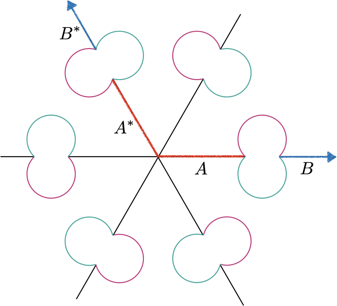
In terms of coordinates we have the following expression
| (96) |
After an analytical continuation and they become
| (97) |
They all lie on the real line of the boundary after the analytical continuation. Our previous formula for the minimal surface still applies. We only need to replace by the cross-ratio for the new points. The result is
| (98) |
This expression is invariant under the reflection .
Appendix B Next order eigenvalue correction to deflected entropy
In this appendix we give a quick derivation of (90). The deflected correlator is (assuming and )
| (99) | ||||
| (100) |
For and we use . For we have . This correlator undergoes a change after inversion . A direct consequence of this is that the contribution from two different crossed regions and are no longer equal but evaluates to . This ensures that the eigenvalues (and hence the entropy) of are invariant as we invert the sign of , as expected from the symmetry of modular flow. It also greatly simplifies our work since we only need to evaluate one scaling region. The eigenfunctions are related to the case
| (101) |
It has a new normalization
| (102) |
Therefore the first order correction to eigenvalues are given by
| (103) |
We have factored to RHS as it restores the symmetry of the integral, as we will see later. Again there are multiple scaling regions to consider, but as in the case only the crossed region and contributes.
Consider and and . The correlator is
| (104) |
The relavent integral is
| (105) |
with and . For the same sign but for we have the integral
| (106) |
with and . One can see the aformentioned symmetry of the correlator with .
These integrals are composed of two different pieces. The first one is absent in :
| (107) | ||||
The second integral is similar to the case but with modified bounds:
| (108) | ||||
Note that we have only kept the terms that is constant as we scale since we know the divergent terms must cancel across different regions from the discussion in Section 4.3.
We conclude that we can write the correction for finite to be
| (109) | ||||
References
- (1) T. Faulkner, T. Hartman, M. Headrick, M. Rangamani and B. Swingle, Snowmass white paper: Quantum information in quantum field theory and quantum gravity, in 2022 Snowmass Summer Study, 3, 2022. 2203.07117.
- (2) H. Casini and M. Huerta, Lectures on entanglement in quantum field theory, 2201.13310.
- (3) H. Casini, M. Huerta, R. C. Myers and A. Yale, Mutual information and the F-theorem, JHEP 10 (2015) 003, [1506.06195].
- (4) S. Dutta and T. Faulkner, A canonical purification for the entanglement wedge cross-section, JHEP 03 (2021) 178, [1905.00577].
- (5) P. Calabrese and A. Lefevre, Entanglement spectrum in one-dimensional systems, Physical Review A 78 (2008) 032329.
- (6) C. Holzhey, F. Larsen and F. Wilczek, Geometric and renormalized entropy in conformal field theory, Nucl. Phys. B 424 (1994) 443–467, [hep-th/9403108].
- (7) P. Calabrese and J. L. Cardy, Entanglement entropy and quantum field theory, J. Stat. Mech. 0406 (2004) P06002, [hep-th/0405152].
- (8) E. Witten, APS Medal for Exceptional Achievement in Research: Invited article on entanglement properties of quantum field theory, Rev. Mod. Phys. 90 (2018) 045003, [1803.04993].
- (9) D. Buchholz, Product states for local algebras, Communications in Mathematical Physics 36 (1974) 287 – 304.
- (10) D. Buchholz and E. H. Wichmann, Causal independence and the energy-level density of states in local quantum field theory, Communications in Mathematical Physics 106 (1986) 321 – 344.
- (11) S. Doplicher and R. Longo, Standard and split inclusions of von neumann algebras., Inventiones mathematicae 75 (1984) 493–536.
- (12) M. Reed and B. Simon, I: Functional Analysis. Methods of Modern Mathematical Physics. Elsevier Science, 1981.
- (13) T. Takayanagi and K. Umemoto, Entanglement of purification through holographic duality, Nature Phys. 14 (2018) 573–577, [1708.09393].
- (14) P. Bueno and H. Casini, Reflected entropy, symmetries and free fermions, JHEP 05 (2020) 103, [2003.09546].
- (15) P. Bueno and H. Casini, Reflected entropy for free scalars, JHEP 11 (2020) 148, [2008.11373].
- (16) H. A. Camargo, L. Hackl, M. P. Heller, A. Jahn and B. Windt, Long Distance Entanglement of Purification and Reflected Entropy in Conformal Field Theory, Phys. Rev. Lett. 127 (2021) 141604, [2102.00013].
- (17) C. Berthiere, H. Chen, Y. Liu and B. Chen, Topological reflected entropy in Chern-Simons theories, Phys. Rev. B 103 (2021) 035149, [2008.07950].
- (18) C. Akers, T. Faulkner, S. Lin and P. Rath, Reflected entropy in random tensor networks, 2112.09122.
- (19) C. Akers, T. Faulkner, S. Lin and P. Rath, The Page Curve for Reflected Entropy, 2201.11730.
- (20) R. Longo and F. Xu, Von Neumann Entropy in QFT, Commun. Math. Phys. 381 (2021) 1031–1054, [1911.09390].
- (21) E. T. Lucas Hackl, Michal P. Heller and Q.-F. Wu, work in progress, .
- (22) P. Hayden, O. Parrikar and J. Sorce, The Markov gap for geometric reflected entropy, JHEP 10 (2021) 047, [2107.00009].
- (23) H. Casini and M. Huerta, Entanglement entropy in free quantum field theory, J. Phys. A 42 (2009) 504007, [0905.2562].
- (24) H. Casini and M. Huerta, Reduced density matrix and internal dynamics for multicomponent regions, Class. Quant. Grav. 26 (2009) 185005, [0903.5284].
- (25) R. Longo, P. Martinetti and K.-H. Rehren, Geometric modular action for disjoint intervals and boundary conformal field theory, Rev. Math. Phys. 22 (2010) 331–354, [0912.1106].
- (26) S. Hollands, On the modular operator of mutli-component regions in chiral CFT, Commun. Math. Phys. 384 (2021) 785–828, [1904.08201].
- (27) T. Faulkner, The Entanglement Renyi Entropies of Disjoint Intervals in AdS/CFT, 1303.7221.
- (28) R. Longo and F. Xu, Relative Entropy in CFT, Adv. Math. 337 (2018) 139–170, [1712.07283].
- (29) M. Takesaki, Tomita’s Theory of Modular Hilbert Algebras and its Applications. Lecture Notes in Mathematics. Springer-Verlag, 1970, 10.1007/bfb0065832.
- (30) C. Yin and Z. Liu, Universal entanglement and correlation measure in two-dimensional conformal field theory, 2211.11952.
- (31) A. Levine, A. Shahbazi-Moghaddam and R. M. Soni, Seeing the entanglement wedge, JHEP 06 (2021) 134, [2009.11305].
- (32) F. Ceyhan and T. Faulkner, Recovering the QNEC from the ANEC, Commun. Math. Phys. 377 (2020) 999–1045, [1812.04683].
- (33) A. Connes, Une classification des facteurs de type , Annales scientifiques de l’École Normale Supérieure 4e série, 6 (1973) 133–252.
- (34) C. M. Bender, S. Orszag and S. A. Orszag, Advanced mathematical methods for scientists and engineers I: Asymptotic methods and perturbation theory, vol. 1. Springer Science & Business Media, 1999.
- (35) T. Faulkner and H. Liu, Condensed matter physics of a strongly coupled gauge theory with quarks: Some novel features of the phase diagram, 0812.4278.
- (36) T. Faulkner, H. Liu, J. McGreevy and D. Vegh, Emergent quantum criticality, Fermi surfaces, and AdS(2), Phys. Rev. D 83 (2011) 125002, [0907.2694].
- (37) E. Azoff and C. Davis, On distances between unitary orbits of self-adjoint operators, Acta Scientiarum Mathematicarum 47 (01, 1984) .
- (38) P. Calabrese and A. Lefevre, Entanglement spectrum in one-dimensional systems, Phys. Rev. A 78 (Sep, 2008) 032329.
- (39) J. Kudler-Flam, Y. Kusuki and S. Ryu, Correlation measures and the entanglement wedge cross-section after quantum quenches in two-dimensional conformal field theories, JHEP 04 (2020) 074, [2001.05501].
- (40) K. Krasnov, Holography and Riemann surfaces, Adv. Theor. Math. Phys. 4 (2000) 929–979, [hep-th/0005106].
- (41) P. Zograf and L. Takhtadzhyan, On uniformization of riemann surfaces and the weil-petersson metric on teichmüller and schottky spaces, Mathematics of the USSR-Sbornik 60 (10, 2007) 297.