跳到论文正文
W Papers独立论文阅读器 arXiv:2211.17155 论文正文 计算阅读时间 · 0%
引用这篇论文根据当前论文元数据生成,正式投稿前建议核对。


License: CC BY 4.0
arXiv:2211.17155v1 [math.ST] 30 Nov 2022

Exponential Concentration for Geometric-Median-of-Means in Non-Positive Curvature Spaces

Ho Yun    Byeong U. Parkabel=e2    mark]bupark@snu.ac.kr

In Euclidean spaces, the empirical mean vector as an estimator of the population mean is known to have polynomial concentration unless a strong tail assumption is imposed on the underlying probability measure. The idea of median-of-means tournament has been considered as a way of overcoming the sub-optimality of the empirical mean vector. In this paper, to address the sub-optimal performance of the empirical mean in a more general setting, we consider general Polish spaces with a general metric, which are allowed to be non-compact and of infinite-dimension. We discuss the estimation of the associated population Fréchet mean, and for this we extend the existing notion of median-of-means to this general setting. We devise several new notions and inequalities associated with the geometry of the underlying metric, and using them we study the concentration properties of the extended notions of median-of-means as the estimators of the population Fréchet mean. We show that the new estimators achieve exponential concentration under only a second moment condition on the underlying distribution, while the empirical Fréchet mean has polynomial concentration. We focus our study on spaces with non-positive Alexandrov curvature since they afford slower rates of convergence than spaces with positive curvature. We note that this is the first work that derives non-asymptotic concentration inequalities for extended notions of the median-of-means in non-vector spaces with a general metric.

keywords
concentration inequalities ; Fréchet mean ; median-of-means estimators ; non-Euclidean geometry ; NPC spaces ; power transform metric

and

??Department of Statistics, Seoul National University, ??, ??

1 Introduction

The notion of a Fréchet mean extends the definition of mean, as a center of probability distribution, to metric space settings. Given a Borel probability measure PP on a metric space (ℳ,d)(\mathcal{M},d) and a functional η:ℳ×ℳ→ℝ\eta:\mathcal{M}\times\mathcal{M}\rightarrow\mathbb{R}, the Fréchet mean (or the barycenter) [22] of PP is any x∗x^{*} such that

x∗∈arg⁡minx∈ℳ∫ℳη(x,y)dP(y).x^{*}\in\argmin_{x\in\mathcal{M}}\int_{\mathcal{M}}\eta(x,y)\,\mathrm{d}P(y). (1)

This accords with the usual definition of the Euclidean mean for ℳ=ℝD\mathcal{M}=\mathbb{R}^{D} when η⁡(x,y)=d​(x,y)2=|x−y|2\eta(x,y)=d(x,y)^{2}=|x-y|^{2}. In this paper, we consider the estimation of the Fréchet mean of a heavy-tailed distribution. Our goal is to find estimators that have better non-asymptotic accuracy than the empirical Fréchet mean,

xn∈arg⁡minx∈ℳ⁡1n​∑i=1nη⁡(x,Xi)x_{n}\in\argmin_{x\in\mathcal{M}}\frac{1}{n}\sum_{i=1}^{n}\eta(x,X_{i}) (2)

when PP is heavy-tailed on ℳ\mathcal{M}. The xnx_{n} is an MM-estimator in a broad sense. The present work is an achievement of this goal for global non-positive curvature (NPC) spaces, also called CAT(0) or Hadamard spaces, that are of finite- or infinite-dimension.

Our coverage with NPC spaces is genuinely broad enough. It includes Hilbert spaces with Euclidean spaces as a special case, and various other types of metric spaces, some of which are listed below.

  • ∙\bullet

    A hyperbolic space ℋD\mathcal{H}_{D} has constant non-positive sectional curvature, which results in rich geometrical features due to explicit expressions for the log\log and exp\exp maps. The deviation of two geodesics in a hyperbolic space accelerates while drifting away from the origin, which allows a natural hierarchical structure in neural networks [24, 50].

  • ∙\bullet

    The space 𝒮D+\mathcal{S}_{D}^{+} of symmetric positive definite matrices has non-constant and non-positive sectional curvature, which appears frequently in diffusion tensor imaging [21, 20]. The space 𝒮D+\mathcal{S}_{D}^{+} is not only a Riemannian manifold, but also an Abelian Lie group with additional algebraic structure [3, 38, 46]. Thus, additive regression modeling is allowed for random elements taking values in 𝒮D+\mathcal{S}_{D}^{+} [39].

  • ∙\bullet

    The Wasserstein space 𝒫2​(ℝ)\mathcal{P}_{2}(\mathbb{R}) over ℝ\mathbb{R} has vanishing Alexandrov curvature [30] and plays a fundamental role in optimal transport [53]. The Wasserstein space has rich applications in modern theories, such as change point detection [28], and Wasserstein regression [14, 54, 25].

Apart from the above-mentioned examples, there are other NPC spaces, such as phylogenetic trees [46, 9], that are of great importance in applications.

A great deal of statistical inference is fundamentally based on the estimation of the Fréchet mean x∗x^{*}. While classical statistics leaned toward the asymptotic behavior of estimators, the derivation of non-asymptotic probability bounds, called concentration or tail inequalities, has drawn increasing attention recently. For an estimator x^=x^​(X1,…,Xn)\hat{x}=\hat{x}(X_{1},\dots,X_{n}) of x∗x^{*}, concentration inequalities for x^\hat{x} are given in the form of

ℙ⁡(d⁡(x^,x∗)≤r⁡(n,Δ))≥1−Δ,\mathbb{P}\left(d(\hat{x},x^{*})\leq r(n,\Delta)\right)\geq 1-\Delta, (3)

where r⁡(n,Δ)r(n,\Delta) is the radius of concentration corresponding to a tail probability level Δ\Delta whose dependence on nn is typically determined by the metric-entropy of ℳ\mathcal{M}. There have been only a few attempts to establish such concentration inequalities when (ℳ,d)(\mathcal{M},d) is not a linear space, and all of them have been restricted to the empirical Fréchet mean x^=xn\hat{x}=x_{n}, to the best of our knowledge. For ℳ=ℝD\mathcal{M}=\mathbb{R}^{D}, it is widely known that the empirical mean xnx_{n} is sub-optimal achieving only polynomial concentration for heavy-tailed PP in the sense that Δ−1=f⁡(n,r⁡(n,Δ))\Delta^{-1}=f(n,r(n,\Delta)) for some ff with f⁡(n,r)f(n,r) for fixed nn being a polynomial function of rr.

A solution to alleviating the sub-optimality of the empirical mean xnx_{n} is to partition {X1,…,Xn}\{X_{1},\ldots,X_{n}\} into a certain number of blocks and then take a ‘median’ of the within-block sample means. This robustifies the empirical mean against heavy-tailed distribution while it inherits its efficiency for light-tailed distribution. The idea was first introduced by [44]. When ℳ=ℝ\mathcal{M}=\mathbb{R}, the resulting estimator, termed as median-of-means, achieves the concentration inequality (3) with r(n,Δ)=C×n−1/2log⁡(1/Δ)r(n,\Delta)=C\times n^{-1/2}\sqrt{\log(1/\Delta)} for some constant C>0C>0 [18]. The one-dimensional result was extended to ℳ=ℝD\mathcal{M}=\mathbb{R}^{D} by [40] developing the idea of ‘median-of-means tournament’. The resulting estimator x^\hat{x}, also termed as median-of-means, was found to achieve a sub-Gaussian performance:

ℙ⁡(‖x^−x∗‖≤C1​tr​(ΣX)n+C2​‖ΣX‖​log⁡(1/Δ)n)≥1−Δ\mathbb{P}\left(\|\hat{x}-x^{*}\|\leq C_{1}\sqrt{\frac{\text{tr}(\Sigma_{X})}{n}}+C_{2}\sqrt{\frac{\|\Sigma_{X}\|\log(1/\Delta)}{n}}\right)\geq 1-\Delta (4)

for some constants C1,C2>0C_{1},C_{2}>0, where ΣX\Sigma_{X} is the covariance matrix and ∥⋅∥\|\cdot\| is the operator norm. The concentration property at (4) is what the empirical mean achieves when XX has a multivariate sub-Gaussian distribution, so the name sub-Gaussian performance. Both results establish exponential concentration in the sense that Δ−1=f⁡(n,r⁡(n,Δ))\Delta^{-1}=f(n,r(n,\Delta)) with f⁡(n,r)f(n,r) for fixed nn being an exponential function of rr. There have been also proposed several other mean estimators satisfying (4) that can be computed in linear time (n​D​log⁡(1/Δ))O⁡(1)(nD\log(1/\Delta))^{O(1)} by using the median-of-means principle, see [27, 15, 17, 36], and other related works on robust mean estimation, e.g. [12, 42].

All the aforementioned works, however, treated Euclidean spaces for η=d2\eta=d^{2} with extensive use of the associated inner product. Apart from the Euclidean cases, there are few works for infinite-dimensional ℳ\mathcal{M}, e.g. [37] for a kernel-enriched domain and [43] for a Banach space, both of which considered η=d2\eta=d^{2}. We are also aware of [29] that studied the case of arbitrary metric spaces. However, the latter work does not use the geometric features of the underlying metric space but assumes certain high-level conditions. The conditions include the existence of an estimator x^\hat{x} and a random distance D​I​S​TDIST on (ℳ,d)(\mathcal{M},d) such that ℙ⁡(d⁡(x^,x∗)≤ε)≥2/3\mathbb{P}(d(\hat{x},x^{*})\leq\varepsilon)\geq 2/3 for some ε>0\varepsilon>0 and ℙ⁡(d⁡(x,y)/2≤D​I​S​T​(x,y)≤2​d​(x,y))≥8/9\mathbb{P}(d(x,y)/2\leq DIST(x,y)\leq 2d(x,y))\geq 8/9 for all x,y∈ℳx,y\in\mathcal{M}. We highlight that the present work is the first to use the median-of-means principle without imposing strong assumptions such as in [29] when ℳ\mathcal{M} is a non-vector space. Our technical development is significantly different from the existing works in the literature. We note that there is no distribution on non-vector spaces corresponding to Gaussian or sub-Gaussian distribution on ℝD\mathbb{R}^{D}, neither are available the notions of trace and operator norm, so that an analogue of the sub-Gaussian performance as at (4) for non-vector spaces does not seem to be possible. Nevertheless, we establish for our estimators exponential concentration in the sense that the inverse of ‘probability regret’ Δ\Delta at (3) is an exponential function of the radius of concentration.

In this paper, we first extend the notion of median-of-means to general metric spaces ℳ\mathcal{M}. Then, we address the problem of robust estimation by taking into account the metric geometry of the underlying space. To this end, we use the CN (‘Courbure Négative’ in French), quadruple and variance inequalities, which are not well known in statistics, instead of the inner product. We show that, when ℳ\mathcal{M} is an NPC space and η⁡(x,y)=d​(x,y)α\eta(x,y)=d(x,y)^{\alpha}, the corresponding geometric-median-of-means estimator achieves exponential concentration for all α∈(1,2]\alpha\in(1,2], under only the second moment condition 𝔼​d​(x∗,X)2<+∞\mathbb{E}\,d(x^{*},X)^{2}<+\infty. In particular, for the treatment of the ‘bridging’ case where α∈(1,2)\alpha\in(1,2), we introduce a further extended notion of the geometric-median-of-means, for which we devise generalized versions of the CN and variance inequalities. Our work is the first that provides concentration inequalities for median-of-means type estimators with explicit constants, when η\eta is not necessarily d2d^{2} or ℳ\mathcal{M} is a possibly infinite-dimensional non-vector space.

We work with (possibly non-compact) NPC spaces for the geometric-median-of-means estimators since the Fréchet mean xnx_{n} has poor performance in such spaces. In fact, the concentration properties of xnx_{n} depend heavily on the compactness and curvature of ℳ\mathcal{M}. For general Polish spaces, an exponential concentration inequality may be established with xnx_{n} if the space is compact [2]. For non-compact geodesic spaces, however, only polynomial concentration is possible with xnx_{n} unless a strong assumption on the tail of PP is imposed. The latter was proved for Euclidean spaces, a special case of non-compact spaces [12]. As for the curvature of the underlying space, xnx_{n} has a poorer rate of convergence for ℳ\mathcal{M} with non-positive curvature than with positive curvature (Sections 3 and 4.3). Curvature and compactness are related in the case where ℳ\mathcal{M} is a Riemannian manifold. The Bonnet-Myers theorem states that, if the sectional curvature of a Riemannian manifold is bounded from below by κ>0\kappa>0, then diam⁡(ℳ)≤π/κ{\rm diam}(\mathcal{M})\leq\pi/\sqrt{\kappa} so that it is compact. To complement the existing works for xnx_{n}, we demonstrate the polynomial concentration of xnx_{n}, as well, for general Polish spaces in Section 3, and for NPC spaces as a specialization of the latter in Section 4. We note that there have been few works on non-asymptotic theory of xnx_{n} for non-Euclidean ℳ\mathcal{M}, although its asymptotic theory has been widely studied [7, 8, 33, 49]. The work in Section 3 for the empirical Fréchet mean xnx_{n} paves our way for developing the main results in Section 5 for the geometric-median-of-means estimators.

Our treatment of NPC spaces relies on the metric geometry of the underlying space ℳ\mathcal{M}, rather than on the differential geometry of ℳ\mathcal{M}. Consequently, the radius of concentration r⁡(n,Δ)r(n,\Delta) in the exponential inequalities in Section 5 does not involve any term related to the structure of the tangential vector space of ℳ\mathcal{M}, which corresponds to ΣX\Sigma_{X} in Lugosi [40] when ℳ=ℝD\mathcal{M}=\mathbb{R}^{D}. We find that assuming 𝔼​d​(x∗,X)2<+∞\mathbb{E}\,d(x^{*},X)^{2}<+\infty is enough to deduce the exponential concentration. The flexibility inherent in our framework thus allows our work to serve as the basic constituent for a wide range of principal methods for non-Euclidean data. In particular, the theoretical development achieved in this paper may be adapted to the robustification of various recent Fréchet regression techniques [39, 14, 54, 25, 47].

2 Assumptions

In this section, we present the main structures of the underlying metric, where we base our theory, and key assumptions on the entropy of the underlying space. The validity of the assumptions will be discussed in Section 4.

Let (ℳ,d)(\mathcal{M},d) be a separable and complete metric space (Polish space). Consider the set of all probability measures on ℳ\mathcal{M} denoted by 𝒫⁡(ℳ)\mathcal{P}(\mathcal{M}). Let PP be a probability measure with finite second moment, i.e.

P∈𝒫2​(ℳ):={P∈𝒫⁡(ℳ):∫ℳd​(x,y)2​𝑑P​(y)<+∞​ for some ​x∈ℳ}.P\in\mathcal{P}_{2}(\mathcal{M}):=\Big\{P\in\mathcal{P}(\mathcal{M}):\int_{\mathcal{M}}d(x,y)^{2}\,\mathrm{d}P(y)<+\infty\,\mbox{ for some }\,x\in\mathcal{M}\Big\}.

We note that, if ∫ℳd​(x,y)2​𝑑P​(y)<+∞\int_{\mathcal{M}}d(x,y)^{2}\,\mathrm{d}P(y)<+\infty for some x∈ℳx\in\mathcal{M}, then it holds for all x∈ℳx\in\mathcal{M}. Let η:ℳ×ℳ→ℝ\eta:\mathcal{M}\times\mathcal{M}\rightarrow\mathbb{R} be a measurable function. Throughout this paper, we assume that there exists x∗∈ℳx^{*}\in\mathcal{M} for which (1) holds and let X1,X2,…,XnX_{1},X_{2},\dots,X_{n} be the i.i.d. observations of a random element XX governed by a probability measure PP, and PnP_{n} be its empirical probability measure. Then, the empirical Fréchet mean xnx_{n} at (2) can be written as

xn∈arg⁡minx∈ℳ∫ℳη(x,y)dPn(y).x_{n}\in\argmin_{x\in\mathcal{M}}\int_{\mathcal{M}}\eta(x,y)\,\mathrm{d}P_{n}(y).

To analyze the deviation of xnx_{n} from x∗x^{*} by making use of the difference of their η\eta-functional values, we introduce two assumptions, the first on η:ℳ×ℳ→ℝ\eta:\mathcal{M}\times\mathcal{M}\rightarrow\mathbb{R} and the second on P∈𝒫2​(ℳ)P\in\mathcal{P}_{2}(\mathcal{M}):

  • (A1)

    Quadruple inequality: There is a nonnegative function l:ℳ×ℳ→[0,+∞)l:\mathcal{M}\times\mathcal{M}\rightarrow[0,+\infty), called growth function, such that, for any y,z,p,q∈ℳy,z,p,q\in\mathcal{M},

    l⁡(y,z)=0⇔y=z,η⁡(y,p)−η⁡(y,q)−η⁡(z,p)+η⁡(z,q)≤2​l​(y,z)⋅d⁡(p,q).\begin{split}&l(y,z)=0\;\Leftrightarrow\;y=z,\\ &\eta(y,p)-\eta(y,q)-\eta(z,p)+\eta(z,q)\leq 2l(y,z)\cdot d(p,q).\end{split}
  • (A2)

    Variance inequality: There exist constants K>0K>0 and β∈(0,2)\beta\in(0,2) such that, for all x∈ℳx\in\mathcal{M},

    l​(x,x∗)2≤K​(∫ℳ(η⁡(x,y)−η⁡(x∗,y))​𝑑P​(y))β.l\left(x,x^{*}\right)^{2}\leq K\left(\int_{\mathcal{M}}\left(\eta(x,y)-\eta\left(x^{*},y\right)\right)\mathrm{d}P(y)\right)^{\beta}.

We note that (A1) and (A2) together imply the uniqueness of the Fréchet mean x∗x^{*}.

Example 1.

Consider the case where ℳ\mathcal{M} is a Hilbert space ℋ\mathcal{H} with an inner product ⟨⋅,⋅⟩\langle\cdot,\cdot\rangle and d⁡(x,y)=‖x−y‖d(x,y)=\|x-y\| for the induced norm ∥⋅∥\|\cdot\| of ⟨⋅,⋅⟩\langle\cdot,\cdot\rangle. Let η=d2\eta=d^{2}. If XX has finite second moment, i.e. 𝔼​d​(x∗,X)2<+∞\mathbb{E}\,d(x^{*},X)^{2}<+\infty, then x∗=𝔼​Xx^{*}=\mathbb{E}X is the unique barycenter of XX in the sense of Bochner integration. Also, it holds that

η⁡(y,p)−η⁡(y,q)−η⁡(z,p)+η⁡(z,q)=(2​⟨y−q,q−p⟩+‖q−p‖2)−(2​⟨z−q,q−p⟩+‖q−p‖2)=2​⟨y−z,q−p⟩≤2​‖y−z‖⋅‖p−q‖.\begin{split}&\eta(y,p)-\eta(y,q)-\eta(z,p)+\eta(z,q)\\ &\qquad=(2\langle y-q,q-p\rangle+\|q-p\|^{2})-(2\langle z-q,q-p\rangle+\|q-p\|^{2})\\ &\qquad=2\langle y-z,q-p\rangle\\ &\qquad\leq 2\|y-z\|\cdot\|p-q\|.\end{split}

Thus, (A1) holds with l=dl=d, and (A2) does with equality holding always for all x∈ℳx\in\mathcal{M} with K=β=1K=\beta=1:

𝔼⁡(η⁡(x,X)−η⁡(x∗,X))=𝔼⁡(2​⟨x∗−X,x−x∗⟩+‖x−x∗‖2)=‖x−x∗‖2.∎\displaystyle\mathbb{E}\left(\eta(x,X)-\eta\left(x^{*},X\right)\right)=\mathbb{E}\left(2\langle x^{*}-X,x-x^{*}\rangle+\|x-x^{*}\|^{2}\right)=\|x-x^{*}\|^{2}.\quad\mbox{\qed}

For curved spaces, the inequality in (A2) may be satisfied, but with equality not holding always for all x∈ℳx\in\mathcal{M} in general, contrary to the Hilbertian case. Moreover, both xnx_{n} and x∗x^{*} do not have a closed form expression for curved metric spaces although xnx_{n} has for Hilbert spaces. Therefore, in order to derive a concentration inequality for xnx_{n}, we need an inequality that gives an upper bound to the discrepancy l⁡(xn,x∗)l(x_{n},x^{*}) between xnx_{n} and x∗x^{*}. The variance inequality (A2) implies that l⁡(xn,x∗)l(x_{n},x^{*}) can be controlled by the positive function η⁡(xn,⋅)−η⁡(x∗,⋅)\eta(x_{n},\cdot)-\eta(x^{*},\cdot), called the empirical excess risk of η\eta:

l​(xn,x∗)2≤K​(∫ℳ(η⁡(xn,y)−η⁡(x∗,y))​𝑑P​(y))β.l\left(x_{n},x^{*}\right)^{2}\leq K\left(\int_{\mathcal{M}}\left(\eta(x_{n},y)-\eta\left(x^{*},y\right)\right)\mathrm{d}P(y)\right)^{\beta}. (5)

For the usual choice η=d2\eta=d^{2}, it turns out that (A1) and (A2) hold with l=d,K=β=1l=d,K=\beta=1 for general NPC spaces ℳ\mathcal{M}, see Section 4.1 for details.

Bounding the right hand side of (5) with a high probability depends on the geometric properties of the class of functions η⁡(x,⋅)−η⁡(x∗,⋅)\eta(x,\cdot)-\eta(x^{*},\cdot) for x∈ℳx\in\mathcal{M}. It turns out that the dependence is through the centered functional ηc\eta_{c} defined by ηc​(x,⋅)=η⁡(x,⋅)−∫ℳη⁡(x,y)​𝑑P​(y)\eta_{c}(x,\cdot)=\eta(x,\cdot)-\int_{\mathcal{M}}\eta(x,y)\mathrm{d}P(y). Put fη​(x,⋅)=ηc​(x,⋅)−ηc​(x∗,⋅)f_{\eta}(x,\cdot)=\eta_{c}(x,\cdot)-\eta_{c}(x^{*},\cdot), x∈ℳx\in\mathcal{M}.

Definition 1.

For δ≥0\delta\geq 0,

ℳη​(δ)={x∈ℳ:∫ℳ(η⁡(x,y)−η⁡(x∗,y))​dP​(y)≤δ},ℱη​(δ)={fη​(x,⋅):x∈ℳη​(δ)},ση2​(δ)=sup{∫ℳfη​(x,y)2​dP​(y):x∈ℳη​(δ)}.\begin{split}&\mathcal{M}_{\eta}(\delta)=\left\{x\in\mathcal{M}:\int_{\mathcal{M}}\left(\eta(x,y)-\eta\left(x^{*},y\right)\right)\mathrm{d}P(y)\leq\delta\right\},\\ &\mathcal{F}_{\eta}(\delta)=\{f_{\eta}(x,\cdot):x\in\mathcal{M}_{\eta}(\delta)\},\\ &\sigma_{\eta}^{2}(\delta)=\sup\left\{\int_{\mathcal{M}}f_{\eta}(x,y)^{2}\,\mathrm{d}P(y):x\in\mathcal{M}_{\eta}(\delta)\right\}.\end{split}
Example 2.

Consider the η\eta and XX in Example 1. Let ΣX:ℋ×ℋ→ℝ\Sigma_{X}:\mathcal{H}\times\mathcal{H}\rightarrow\mathbb{R} be the covariance operator of XX defined by ΣX​(x,y)=𝔼⁡(⟨x,X−x∗⟩​⟨y,X−x∗⟩)\Sigma_{X}(x,y)=\mathbb{E}\,\left(\langle x,X-x^{*}\rangle\langle y,X-x^{*}\rangle\right) and λm​a​x\lambda_{max} be its largest eigenvalue. From Example 1, it is straightforward to see that ℳη​(δ)=B⁡(x∗,δ)\mathcal{M}_{\eta}(\delta)=B(x^{*},\sqrt{\delta}) and 𝔼​η​(x,X)=tr⁡(ΣX)+‖x−x∗‖2\mathbb{E}\,\eta(x,X)=\operatorname{tr}(\Sigma_{X})+\|x-x^{*}\|^{2}, where B⁡(x,r)B(x,r) denotes the ball centered at xx with radius rr, tr⁡(ΣX)=∑kΣX​(ek,ek)\operatorname{tr}(\Sigma_{X})=\sum_{k}\Sigma_{X}(e_{k},e_{k}) and {ek:k≥1}\{e_{k}:k\geq 1\} is an arbitrary orthonormal basis of ℋ\mathcal{H}. Let ∥⋅∥2,P\|\cdot\|_{2,P} be defined by ‖f‖2,P2=𝔼​f​(X)2\|f\|_{2,P}^{2}=\mathbb{E}\,f(X)^{2}. Then,

ηc​(x,y)=‖x−y‖2−‖x−x∗‖2−tr⁡(ΣX),fη​(x,y)=2​⟨x−x∗,x∗−y⟩,‖fη​(x,⋅)−fη​(y,⋅)‖2,P2=4​𝔼​(⟨x−y,X−x∗⟩2)=4​ΣX​(x−y,x−y).\begin{split}\eta_{c}(x,y)&=\|x-y\|^{2}-\|x-x^{*}\|^{2}-\operatorname{tr}(\Sigma_{X}),\\ f_{\eta}(x,y)&=2\langle x-x^{*},x^{*}-y\rangle,\\ \|f_{\eta}(x,\cdot)-f_{\eta}(y,\cdot)\|^{2}_{2,P}&=4\,\mathbb{E}\,\left(\langle x-y,X-x^{*}\rangle^{2}\right)=4\,\Sigma_{X}(x-y,x-y).\end{split}

Note that fη​(x,⋅):ℋ→ℝf_{\eta}(x,\cdot):\mathcal{H}\rightarrow\mathbb{R} is an affine function and fη​(x∗,⋅)≡0≡fη​(⋅,x∗)f_{\eta}(x^{*},\cdot)\equiv 0\equiv f_{\eta}(\cdot,x^{*}). Also, from the Cauchy-Schwarz inequality, we have

ση2​(δ)=sup{4​𝔼​(⟨x−x∗,X−x∗⟩2):x∈B⁡(x∗,δ)}=sup{4​ΣX​(x−x∗,x−x∗):x∈B⁡(x∗,δ)}=4​δ⋅λm​a​x.∎\begin{split}\sigma_{\eta}^{2}(\delta)&=\sup\left\{4\mathbb{E}(\langle x-x^{*},X-x^{*}\rangle^{2}):x\in B(x^{*},\sqrt{\delta})\right\}\\ &=\sup\left\{4\Sigma_{X}(x-x^{*},x-x^{*}):x\in B(x^{*},\sqrt{\delta})\right\}\\ &=4\delta\cdot\lambda_{max}.\quad\mbox{\qed}\end{split}

Under the assumptions (A1) and (A2), it holds that

supx∈ℳη​(δ)fη​(x,y)=supx∈ℳη​(δ)∫ℳ(η⁡(x,y)−η⁡(x∗,y)−η⁡(x,z)+η⁡(x∗,z))​dP​(z)≤2​supx∈ℳη​(δ)∫ℳl⁡(x,x∗)​d​(y,z)​dP​(z)≤2​K​δβ​∫ℳd⁡(y,z)​dP​(z)=:Hδ,η​(y).\displaystyle\begin{split}\sup_{x\in\mathcal{M}_{\eta}(\delta)}f_{\eta}(x,y)&=\sup_{x\in\mathcal{M}_{\eta}(\delta)}\int_{\mathcal{M}}\left(\eta(x,y)-\eta(x^{*},y)-\eta(x,z)+\eta(x^{*},z)\right)\,\mathrm{d}P(z)\\ &\leq 2\sup_{x\in\mathcal{M}_{\eta}(\delta)}\int_{\mathcal{M}}l(x,x^{*})d(y,z)\,\mathrm{d}P(z)\\ &\leq 2\sqrt{K\delta^{\beta}}\int_{\mathcal{M}}d(y,z)\,\mathrm{d}P(z)=:H_{\delta,\eta}(y).\end{split} (6)

By definition Hδ,ηH_{\delta,\eta} envelops the class ℱη​(δ)\mathcal{F}_{\eta}(\delta) of functions under the assumptions (A1) and (A2). Let ∥⋅∥2,Pn\|\cdot\|_{2,P_{n}} be defined by

‖f‖2,Pn2=n−1​∑i=1nf​(Xi)2,f:ℳ→ℝ.\|f\|_{2,P_{n}}^{2}=n^{-1}\sum_{i=1}^{n}f(X_{i})^{2},\quad f:\mathcal{M}\rightarrow\mathbb{R}.

Note that ∥⋅∥2,Pn\|\cdot\|_{2,P_{n}} is a pseudo metric. To analyze high probability concentration, toward zero, of the right hand side of (5), we consider the following assumption on the ∥⋅∥2,Pn\|\cdot\|_{2,P_{n}}-metric entropy of ℳ\mathcal{M}. For a totally bounded subset 𝒮\mathcal{S} of a metric space (ℱ,d)(\mathcal{F},d), we let N⁡(τ,𝒮,d)N(\tau,\mathcal{S},d) denote the minimal number of balls with radius τ\tau that cover 𝒮\mathcal{S}, and call it τ\tau-covering number.

  • (B1)

    Finite-dimensional ℳ\mathcal{M}: There are some constants A,D>0A,D>0 such that, for any δ>0\delta>0 and n∈ℕn\in\mathbb{N},

    N(τ∥Hδ,η∥2,Pn,ℱη(δ),∥⋅∥2,Pn))≤(Aτ)D,0<τ≤1,N\left(\tau\|H_{\delta,\eta}\|_{2,P_{n}},\mathcal{F}_{\eta}(\delta),\|\cdot\|_{2,P_{n}})\right)\leq\left(\frac{A}{\tau}\right)^{D},\quad 0<\tau\leq 1,

The constant DD in the assumption (B1) is related to the index of VC(Vapnik-C̆ervonenkis)-type class of functions, which appears frequently in M-estimation. According to the common definition [26], ℱη​(δ)\mathcal{F}_{\eta}(\delta) is of VC-type with respect to Hδ,ηH_{\delta,\eta} if

supQ∈𝒫⁡(ℳ)N(τ∥Hδ,η∥2,Q,ℱη(δ),∥⋅∥2,Q))≤(Aτ)Dvc\displaystyle\sup_{Q\in\mathcal{P}(\mathcal{M})}N\left(\tau\|H_{\delta,\eta}\|_{2,Q},\mathcal{F}_{\eta}(\delta),\|\cdot\|_{2,Q})\right)\leq\left(\frac{A}{\tau}\right)^{D_{\rm vc}} (7)

for some constants A,Dvc>0A,D_{\rm vc}>0. The constant DvcD_{\rm vc}, termed as VC index, may not equal the dimension of ℳ\mathcal{M} in general, but is usually larger, and (7) implies (B1) with D=DvcD=D_{\rm vc}, the latter being what we actually need in our framework. Because of the implication, ℱη​(δ)\mathcal{F}_{\eta}(\delta) with (B1) may be regarded as a weak VC-type class of functions, and DD as a weak VC index. In Proposition 3 given later in Section 4 we show that (B1) holds with D=dim⁡(ℳ)D=\operatorname{dim}(\mathcal{M}) in the case where ℳ\mathcal{M} is an NPC space with dim⁡(ℳ)<+∞\operatorname{dim}(\mathcal{M})<+\infty and η=d2\eta=d^{2}.

For infinite-dimensional scenarios, we make the following assumption on the geometric complexity of ℳ\mathcal{M}.

  • (B2)

    Infinite-dimensional ℳ\mathcal{M}: There are some constants A,ζ>0A,\zeta>0 such that, for any δ>0\delta>0 and n∈ℕn\in\mathbb{N},

    logN(τ∥Hδ,η∥2,Pn,ℱη(δ),∥⋅∥2,Pn))≤Aτ2​ζ,0<τ≤1.\log N\left(\tau\|H_{\delta,\eta}\|_{2,P_{n}},\mathcal{F}_{\eta}(\delta),\|\cdot\|_{2,P_{n}})\right)\leq\frac{A}{\tau^{2\zeta}},\quad 0<\tau\leq 1.

The constant ζ\zeta describes how quickly the covering number grows as τ\tau decreases. For probability measures PP with non-compact support, the complexity constant depends largely on the curvature of ℳ\mathcal{M}. Here and throughout the paper, ‘curvature’ means sectional curvature for Riemannian manifolds, and Alexandrov curvature for general metric spaces. When η=d2\eta=d^{2}, we get that ζ=1\zeta=1 for Hilbert spaces ℳ\mathcal{M}, ζ≤1\zeta\leq 1 for geodesic spaces with positive curvature, and ζ≥1\zeta\geq 1 for geodesic spaces with non-positive curvature, see Section 4.3. Based on this, we call ζ\zeta the curvature complexity of ℳ\mathcal{M}.

3 Empirical Fréchet means

In this section, we present two theorems that establish polynomial concentration for empirical Fréchet means under the assumptions (A1), (A2), (B1) and (B2) in the case where ℳ\mathcal{M} is a general Polish space. The theorems are used in developing exponential concentration for geometric-median-of-means estimators to be introduced in Section 5. Throughout this section, we assume that PP has finite second moment, i.e., σX2:=𝔼​d​(x∗,X)2<+∞\sigma_{X}^{2}:=\mathbb{E}\,d(x^{*},X)^{2}<+\infty.

Theorem 1.

Assume (A1), (A2) and (B1), and let (K,β)(K,\beta) and (A,D)(A,D) be the constant pairs that appear in (A2) and (B1), respectively. Then, for all n∈ℕn\in\mathbb{N} and Δ∈(0,1)\Delta\in(0,1),

l⁡(xn,x∗)≤CΔ⋅(σXn)β2−β\displaystyle l(x_{n},x^{*})\leq C_{\Delta}\cdot\left(\frac{\sigma_{X}}{\sqrt{n}}\right)^{\frac{\beta}{2-\beta}}

with probability at least 1−Δ1-\Delta, where CΔC_{\Delta} is given by

CΔ=K12−β​{32​(24​A​D+2Δ)}β2−β.C_{\Delta}=K^{\frac{1}{2-\beta}}\left\{32\left(24\sqrt{AD}+\sqrt{\frac{2}{\Delta}}\right)\right\}^{\frac{\beta}{2-\beta}}.

In the case where ℳ\mathcal{M} is an NPC space to be introduced in the next section, choosing η=d2\eta=d^{2} gives l=dl=d and K=β=1K=\beta=1, see Section 4.1. In this case, Theorem 1 provides an upper bound of order σX/n​Δ\sigma_{X}/\sqrt{n\Delta} for d⁡(xn,x∗)d(x_{n},x^{*}). Note that, in the trivial case where ℳ=ℝD\mathcal{M}=\mathbb{R}^{D} with d⁡(x,y)=|x−y|d(x,y)=|x-y|, an application of the Chebyshev inequality gives

ℙ⁡(|xn−x∗|≤σXn​Δ)≥1−Δ.\mathbb{P}\left(|x_{n}-x^{*}|\leq\frac{\sigma_{X}}{\sqrt{n\Delta}}\right)\geq 1-\Delta.

Here and throughout this paper, |⋅||\cdot| denotes the Euclidean norm. The extra factor CΔC_{\Delta} in Theorem 1 is a price we pay for the complexity of ℳ\mathcal{M} to deal with general metric spaces. The following theorem is for infinite-dimensional scenarios with the assumption (B2).

Theorem 2.

Assume (A1), (A2) and (B2), and let (K,β)(K,\beta) and (A,ζ)(A,\zeta) be the constant pairs that appear in (A2) and (B2), respectively. Then, there is a universal constant CA,ζC_{A,\zeta} depending only on A>0A>0 and ζ>0\zeta>0 such that, for all n∈ℕn\in\mathbb{N} and Δ∈(0,1)\Delta\in(0,1),

l⁡(xn,x∗)≤{K12−β(CA,ζ⋅1n1/2⋅σXΔ)β2−β,if​  0<ζ<1K12−β(CA,1⋅log⁡nn1/2⋅σXΔ)β2−β,if​ζ=1K12−β(CA,ζ⋅1n1/2​ζ⋅σXΔ)β2−β,if​ζ>1\displaystyle l(x_{n},x^{*})\leq\begin{cases}\displaystyle K^{\frac{1}{2-\beta}}\left(C_{A,\zeta}\cdot\frac{1}{n^{1/2}}\cdot\frac{\sigma_{X}}{\sqrt{\Delta}}\right)^{\frac{\beta}{2-\beta}},\quad&\mbox{if}\;\;0<\zeta<1\\ \quad\\[-17.07164pt] \displaystyle K^{\frac{1}{2-\beta}}\left(C_{A,1}\cdot\frac{\log n}{n^{1/2}}\cdot\frac{\sigma_{X}}{\sqrt{\Delta}}\right)^{\frac{\beta}{2-\beta}},\quad&\text{if}\;\;\zeta=1\\ \quad\\[-17.07164pt] \displaystyle K^{\frac{1}{2-\beta}}\left(C_{A,\zeta}\cdot\frac{1}{n^{1/2\zeta}}\cdot\frac{\sigma_{X}}{\sqrt{\Delta}}\right)^{\frac{\beta}{2-\beta}},\quad&\text{if}\;\;\zeta>1\\ \end{cases}

with probability at least 1−Δ1-\Delta.

An explicit form of the constant CA,ζC_{A,\zeta} in Theorem 2 may be found in the proof of the theorem in Section A.1. The theorem demonstrates that the consistency of the empirical Fréchet mean xnx_{n} continues to hold for infinite-dimensional (ℳ,d)(\mathcal{M},d), but with slower rates of convergence to x∗x^{*} for increasing nn when ζ≥1\zeta\geq 1, compared to the finite-dimensional case in Theorem 1. It shows that, for infinite-dimensional geodesic spaces ℳ\mathcal{M}, decreasing the curvature of ℳ\mathcal{M} results in slowing down the rate of convergence of xnx_{n} to x∗x^{*} since the curvature complexity ζ\zeta gets larger as the curvature decreases. This implies that the rate is slower for ℳ\mathcal{M} with non-positive curvature than with positive curvature. We note that, for the finite-dimensional case, the rate of convergence of xnx_{n} does not depend on the curvature, as is shown in Theorem 1. The constant AA in CΔC_{\Delta}, however, gets larger as the curvature of ℳ\mathcal{M} decreases in the case where ℳ\mathcal{M} is a Riemannian manifold and η=d2\eta=d^{2}, see Section 4.3.

Theorems 1 and 2 reveal that the empirical Fréchet mean achieves only polynomial concentration speeds. In Section 5 we discuss in depth alternative estimators that have exponential speeds, basically replacing 1/Δ1/\Delta by log⁡(1/Δ)\log(1/\Delta) in the concentration inequalities.

4 Consideration of assumptions

In this section, we discuss the validity of the assumptions (A1), (A2), (B1) and (B2) for non-positive curvature (NPC) spaces. We also derive generalized versions of the CN and variance inequalities.

Definition 2.

A Polish space (ℳ,d)(\mathcal{M},d) is called an (global) NPC space if for any x0,x1∈ℳx_{0},x_{1}\in\mathcal{M}, there exists y∈ℳy\in\mathcal{M} such that

d​(z,y)2≤12​d​(z,x0)2+12​d​(z,x1)2−14​d​(x0,x1)2,z∈ℳ.d(z,y)^{2}\leq\frac{1}{2}d(z,x_{0})^{2}+\frac{1}{2}d(z,x_{1})^{2}-\frac{1}{4}d(x_{0},x_{1})^{2},\quad z\in\mathcal{M}.
Example 3.

Any Hilbert space (ℋ,⟨⋅,⋅⟩)(\mathcal{H},\langle\cdot,\cdot\rangle) is an NPC space: for any x0,x1,z∈ℳx_{0},x_{1},z\in\mathcal{M}

12​d​(z,x0)2+12​d​(z,x1)2−14​d​(x0,x1)2=14​(2​‖z−x0‖2+2​‖z−x1‖2−‖(z−x0)−(z−x1)‖2)=14​‖(z−x0)+(z−x1)‖2=d​(z,x0+x12)2.∎\begin{split}\frac{1}{2}d(z,x_{0})^{2}+\frac{1}{2}d(z,x_{1})^{2}-\frac{1}{4}d(x_{0},x_{1})^{2}&=\frac{1}{4}\left(2\|z-x_{0}\|^{2}+2\|z-x_{1}\|^{2}-\|(z-x_{0})-(z-x_{1})\|^{2}\right)\\ &=\frac{1}{4}\,\|(z-x_{0})+(z-x_{1})\|^{2}\\ &=d\left(z,\frac{x_{0}+x_{1}}{2}\right)^{2}.\quad\mbox{\qed}\end{split}

Throughout this section, ℳ\mathcal{M} is an NPC space. Also, when there is no confusion, with an abuse of terminology, ‘Riemannian manifold’ means a smooth, complete and connected finite-dimensional Riemannian manifold. By the Hopf-Rinow Theorem, such a Riemannian manifold is geodesically complete.

4.1 Common choice η=d2\eta=d^{2}

Let us first discuss some properties of NPC spaces when η⁡(x,y)=d​(x,y)2\eta(x,y)=d(x,y)^{2}. The geometry of metric measure spaces with non-positive curvature is mainly developed by Sturm [49]. Note that the existence and uniqueness of the Fréchet mean for any probability measure are guaranteed for such spaces.

We have seen in Example 1 that, for Hilbert spaces, the inner product structure allows us to easily verify (A1) and the equality in (A2) with l=dl=d, K=β=1K=\beta=1. For curved spaces, however, d​(x,y)2−d​(x∗,y)2d(x,y)^{2}-d(x^{*},y)^{2} cannot be expressed nicely, thus our assumptions (A1) and (A2) may not be easy to check. For example, for Riemannian manifolds ℳ\mathcal{M}, the relationship between the embedded distance ‖logp⁡x−logp⁡y‖\|\log_{p}x-\log_{p}y\| for p,x,y∈ℳp,x,y\in\mathcal{M} and the original distance d⁡(x,y)d(x,y) depends considerably on the curvature, see Remark 1 below. Nevertheless, using the fact that the geodesic deviation accelerates as two geodesics move further away from the origin, one may prove the following inequalities for global NPC spaces ℳ\mathcal{M}, see [49] for details.

  • CN inequality: For any y∈ℳy\in\mathcal{M} and for any geodesic γ:[0,1]→ℳ\gamma:[0,1]\rightarrow\mathcal{M},

    d​(γt,y)2≤(1−t)​d​(γ0,y)2+t​d​(γ1,y)2−t⁡(1−t)​d​(γ0,γ1)2,t∈[0,1].d(\gamma_{t},y)^{2}\leq(1-t)d(\gamma_{0},y)^{2}+t\,d(\gamma_{1},y)^{2}-t(1-t)d(\gamma_{0},\gamma_{1})^{2},\quad t\in[0,1].
  • Quadruple inequality: For any y,z,p,q∈ℳy,z,p,q\in\mathcal{M},

    d​(y,p)2−d​(z,p)2−d​(y,q)2+d​(z,q)2≤2​d​(y,z)​d​(p,q).d(y,p)^{2}-d(z,p)^{2}-d(y,q)^{2}+d(z,q)^{2}\leq 2d(y,z)d(p,q).
  • Variance inequality: For any x∈ℳx\in\mathcal{M} and for any P∈𝒫2​(ℳ)P\in\mathcal{P}_{2}(\mathcal{M}),

    d​(x,x∗)2≤∫ℳ(d​(x,y)2−d​(x∗,y)2)​𝑑P​(y).d\left(x,x^{*}\right)^{2}\leq\int_{\mathcal{M}}\left(d(x,y)^{2}-d\left(x^{*},y\right)^{2}\right)\mathrm{d}P(y).

Here, ‘CN’ stands for Courbure Négative in French. Therefore, not only for Hilbert spaces but also for NPC spaces, our assumptions (A1) and (A2) are satisfied with K=β=1K=\beta=1, l=dl=d for the usual choice η⁡(x,y)=d​(x,y)2\eta(x,y)=d(x,y)^{2}.

Remark 1.

We note that η=d2\eta=d^{2} satisfies the Hamilton-Jacobi equation, see (14.29) in [53], and the homogeneous Taylor polynomial of order 4 for η\eta gives the following formula: for any p∈ℳp\in\mathcal{M} and v,w∈Tp​ℳv,w\in T_{p}\mathcal{M},

d​(expp⁡(t​v),expp⁡(t​w))2=‖v−w‖2⋅t2−13​Riem⁡(v,w,w,v)⋅t4+O⁡(t5),d\left(\exp_{p}(tv),\exp_{p}(tw)\right)^{2}=\|v-w\|^{2}\cdot t^{2}-\frac{1}{3}\operatorname{Riem}(v,w,w,v)\cdot t^{4}+O(t^{5}),

where ‘Riem\operatorname{Riem}’ stands for the Riemannian curvature tensor.

4.2 Cases with η=dα\eta=d^{\alpha}

Here, we consider the choice η=dα\eta=d^{\alpha}, or equivalently η=dα2\eta=d_{\alpha}^{2} with dα=dα/2d_{\alpha}=d^{\alpha/2}, for α∈(1,2]\alpha\in(1,2]. We note that the Fréchet mean x∗x^{*} corresponding to α=1\alpha=1 is analogous to the conventional median for ℳ=ℝ\mathcal{M}=\mathbb{R}, thus is often called Fréchet median. We exclude the case α=1\alpha=1 in our discussion, however, for the reason to be given shortly. We also note that dαd_{\alpha} is a metric for α∈(1,2]\alpha\in(1,2], and is often called power transform metric. The associated Fréchet mean is called α\alpha-power Fréchet mean. With a slight abuse of notation we continue to denote it by x∗x^{*} throughout this paper.

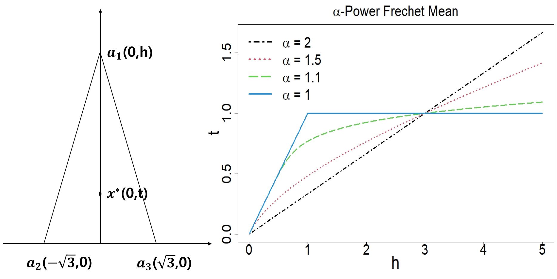
Fig. 1 illustrates the α\alpha-power Fréchet means for several α∈[1,2]\alpha\in[1,2] when ℳ=ℝ2\mathcal{M}=\mathbb{R}^{2}, d⁡(x,y)=|x−y|d(x,y)=|x-y| and PP has the equal probability mass 1/31/3 at three points a1=(0,h),a2=(−3,0),a3=(3,0)a_{1}=(0,h),\,a_{2}=(-\sqrt{3},0),\,a_{3}=(\sqrt{3},0). The right panel depicts tt in x∗=(0,t)x^{*}=(0,t) as a function of hh. For α=2\alpha=2, x∗=(a1+a2+a3)/3=(0,h/3)x^{*}=(a_{1}+a_{2}+a_{3})/3=(0,h/3) becomes most sensitive to the change of a1=(0,h)a_{1}=(0,h) from a certain point on the scale of hh. For α=1\alpha=1, x∗=arg⁡minx∈ℝ2⁡xa1¯+xa2¯+xa3¯x^{*}=\argmin_{x\in\mathbb{R}^{2}}\overline{xa_{1}}+\overline{xa_{2}}+\overline{xa_{3}}, known as the Fermat point, is invariant for h≥1h\geq 1. As the cases α=1.1\alpha=1.1 and α=1.5\alpha=1.5 demonstrate, x∗x^{*} for α∈(1,2)\alpha\in(1,2) is resistent to outlying a1=(0,h)a_{1}=(0,h) to a certain extent depending on α\alpha: the smaller α\alpha is, the more it resists.

Fig. 1 also indicates that all α\alpha-power Fréchet means for different values of α\alpha meet at (0,1)(0,1) when a1=(0,3)a_{1}=(0,3). This is not a coincidence. Proposition S.1 in the Supplementary Material shows that, if the underlying probability measure PP is invariant under rotation around a point zz, then zz is the unique α\alpha-power Fréchet mean for all α≥1\alpha\geq 1.

Refer to caption
Figure 1: The left panel depicts the positions of the α\alpha-power Fréchet mean x∗x^{*} and the three points a1,a2,a3a_{1},\,a_{2},\,a_{3} having equal mass. The right panel shows the change of x∗x^{*} as a1a_{1} moves with a2a_{2} and a3a_{3} staying fixed, for α=1/1.1/1.5/2\alpha=1/1.1/1.5/2 (solid/dashed/dotted/dot-dashed).

The rates of convergence for α\alpha-power Fréchet means are studied for NPC spaces with α∈[1,2]\alpha\in[1,2] in Schötz [48]. In the latter work it is proved that the assumption (A1) holds with l⁡(⋅,⋅)=α​2−α+1​d​(⋅,⋅)α−1l(\cdot,\cdot)=\alpha 2^{-\alpha+1}d(\cdot,\cdot)^{\alpha-1}: for any y,z,p,q∈ℳy,z,p,q\in\mathcal{M},

d​(y,p)α−d​(z,p)α−d​(y,q)α+d​(z,q)α≤α​2−α+2​d​(y,z)α−1​d​(p,q),α∈[1,2].d(y,p)^{\alpha}-d(z,p)^{\alpha}-d(y,q)^{\alpha}+d(z,q)^{\alpha}\leq\alpha 2^{-\alpha+2}d(y,z)^{\alpha-1}d(p,q),\quad\alpha\in[1,2]. (8)

Moreover, according to Appendix E in Schötz [48], no growth function satisfying (A1) exists for α>2\alpha>2 and 0<α<10<\alpha<1. For α=1\alpha=1, (8) implies (A1) with the growth function l⁡(y,z)=I⁡(y≠z)l(y,z)=I(y\neq z), but with this the assumption (A2) makes no sense, so that Theorems 1 and 2 are not meaningful for η=d\eta=d. For the case where α=1\alpha=1, Bac̆ák [4] provided some results analogous to Theorems 1 and 2. Bac̆ák [5, 6] also introduced stochastic proximal point algorithms (PPA) to compute Fréchet medians in NPC spaces.

In the next two propositions we derive generalized CN and variance inequalities for α∈(1,2]\alpha\in(1,2]. Thus, the theorems in Section 3 remain valid for α\alpha-power Fréchet means as well.

Proposition 1 (Power transform CN inequality).

Let γ:[0,1]→ℳ\gamma:[0,1]\rightarrow\mathcal{M} be a geodesic and α∈[1,2]\alpha\in[1,2]. Then, it holds that, for any δ≥0\delta\geq 0, t∈[0,1]t\in[0,1] and z∈ℳz\in\mathcal{M},

d​(γt,z)α\displaystyle d(\gamma_{t},z)^{\alpha} ≤(1+δ)1−α/2​[(1−t)α/2​d​(γ0,z)α+tα/2​d​(γ1,z)α]\displaystyle\leq(1+\delta)^{1-\alpha/2}\left[(1-t)^{\alpha/2}d(\gamma_{0},z)^{\alpha}+t^{\alpha/2}d(\gamma_{1},z)^{\alpha}\right]
−δ1−α/2​[t⁡(1−t)​d​(γ0,γ1)2]α/2.\displaystyle\hskip 56.9055pt-\delta^{1-\alpha/2}\left[t(1-t)d(\gamma_{0},\gamma_{1})^{2}\right]^{\alpha/2}.

Our result in Proposition 1 reduces to the CN inequality in Section 4.1 when α=2\alpha=2. It is believed to be a sharp generalization since it is derived from the CN inequality in Section 4.1 and a version of Hölder’s inequality, both of which are sharp. When given three points x,y,z∈ℳx,y,z\in\mathcal{M}, Proposition 1 enables us to get an upper bound for the power transform metric η⁡(⋅,z)=d​(⋅,z)α\eta(\cdot,z)=d(\cdot,z)^{\alpha} along the geodesic from xx to yy, which does not seem to be feasible for general η\eta. We will illustrate how to use this inequality in a concrete way in the proof of the following proposition, and also in the proofs of the concentration inequalities given in Theorems 6 and 7 later in Section 5.2.

To state the second proposition, for α>0\alpha>0 we let

𝒫α​(ℳ):={P∈𝒫:∫ℳd​(x,y)α​𝑑P​(y)<+∞​ for some ​x∈ℳ}.\mathcal{P}_{\alpha}(\mathcal{M}):=\Big\{P\in\mathcal{P}:\int_{\mathcal{M}}d(x,y)^{\alpha}\mathrm{d}P(y)<+\infty\,\mbox{ for some }\,x\in\mathcal{M}\Big\}.

For P∈𝒫α​(ℳ)P\in\mathcal{P}_{\alpha}(\mathcal{M}), define Fα​(⋅)=∫ℳd​(⋅,y)α​𝑑P​(y)F_{\alpha}(\cdot)=\int_{\mathcal{M}}d(\cdot,y)^{\alpha}\mathrm{d}P(y) and

bα​(x)=supt∈(0,1]Fα​(γtx)−{tα/2+(1−t)α/2}​Fα​(x∗)tα/2​d​(x,x∗)α,x∈ℳ∖{x∗},b_{\alpha}(x)=\sup_{t\in(0,1]}\frac{F_{\alpha}(\gamma^{x}_{t})-\left\{t^{\alpha/2}+(1-t)^{\alpha/2}\right\}F_{\alpha}(x^{*})}{t^{\alpha/2}d(x,x^{*})^{\alpha}},\quad x\in\mathcal{M}\setminus\{x^{*}\},

where γx:[0,1]→ℳ\gamma^{x}:[0,1]\rightarrow\mathcal{M} is the geodesic from x∗x^{*} to xx.

Proposition 2 (Power transform variance inequality).

Let α∈[1,2]\alpha\in[1,2] and P∈𝒫α​(ℳ)P\in\mathcal{P}_{\alpha}(\mathcal{M}). If bα​(x)>0b_{\alpha}(x)>0, then

d​(x,x∗)α≤1bα​(x)​∫ℳ(d​(x,y)α−d​(x∗,y)α)​𝑑P​(y),x∈ℳ∖{x∗}.d\left(x,x^{*}\right)^{\alpha}\leq\frac{1}{b_{\alpha}(x)}\int_{\mathcal{M}}\left(d(x,y)^{\alpha}-d\left(x^{*},y\right)^{\alpha}\right)\mathrm{d}P(y),\quad x\in\mathcal{M}\setminus\{x^{*}\}.

Therefore, if Bα:=infx∈ℳ∖{x∗}bα​(x)>0B_{\alpha}:=\inf_{x\in\mathcal{M}\setminus\{x^{*}\}}b_{\alpha}(x)>0, then for any x∈ℳx\in\mathcal{M},

d​(x,x∗)α≤1Bα​∫ℳ(d​(x,y)α−d​(x∗,y)α)​𝑑P​(y).d\left(x,x^{*}\right)^{\alpha}\leq\frac{1}{B_{\alpha}}\int_{\mathcal{M}}\left(d(x,y)^{\alpha}-d\left(x^{*},y\right)^{\alpha}\right)\mathrm{d}P(y).

Proposition 2 tells that, in order to establish the power transform variance inequality, it suffices to check that, for all x∈ℳ∖{x∗}x\in\mathcal{M}\setminus\{x^{*}\}, Fα​(γtx)F_{\alpha}(\gamma^{x}_{t}) gets apart from (tα/2+(1−t)α/2)​Fα​(x∗)(t^{\alpha/2}+(1-t)^{\alpha/2})F_{\alpha}(x^{*}) by more than a positive constant multiple of tα2​d​(x,x∗)αt^{\frac{\alpha}{2}}d(x,x^{*})^{\alpha}, at some point γtx\gamma^{x}_{t} along the geodesic from x∗x^{*} to xx. Note that Fα​(x∗)=infx∈ℳFα​(x)F_{\alpha}(x^{*})=\inf_{x\in\mathcal{M}}\,F_{\alpha}(x) and tα/2+(1−t)α/2≥1t^{\alpha/2}+(1-t)^{\alpha/2}\geq 1 for all t∈[0,1]t\in[0,1]. For the common choice η=d2\eta=d^{2}, i.e. α=2\alpha=2, it follows from the (power transform) CN inequality that, for any x∈ℳ∖{x∗}x\in\mathcal{M}\setminus\{x^{*}\},

b2​(x)=supt∈(0,1]F2​(γtx)−F2​(x∗)t⋅d​(x,x∗)2≥supt∈(0,1]t2⋅d​(x,x∗)2t⋅d​(x,x∗)2=1.b_{2}(x)=\sup_{t\in(0,1]}\frac{F_{2}(\gamma^{x}_{t})-F_{2}(x^{*})}{t\cdot d(x,x^{*})^{2}}\geq\sup_{t\in(0,1]}\frac{t^{2}\cdot d(x,x^{*})^{2}}{t\cdot d(x,x^{*})^{2}}=1.

Thus, we may take B2=1B_{2}=1 in this case and the proposition gives the usual variance inequality in Section 4.1. For η=dα\eta=d^{\alpha} with α∈(1,2]\alpha\in(1,2] in general, if P∈𝒫α​(ℳ)P\in\mathcal{P}_{\alpha}(\mathcal{M}) satisfies Bα>0B_{\alpha}>0, then (A1) and (A2) hold with l⁡(y,z)=α​2−α+1​d​(y,z)α−1,K=α2​2−2​α+2​Bα−2+2/αl(y,z)=\alpha 2^{-\alpha+1}d(y,z)^{\alpha-1},K=\alpha^{2}2^{-2\alpha+2}B_{\alpha}^{-2+2/\alpha} and β=2−2/α∈(0,1]\beta=2-2/\alpha\in(0,1]. Thus, in this general case as well, Theorems 1 and 2 hold under the entropy conditions (B1) and (B2), respectively. The theorems give that

ℙ⁡(d⁡(xn,x∗)≤64​(Kαα/2α)1/(α−1)⋅(24​A​D+2Δ)⋅σXn)≥1−Δ\displaystyle\mathbb{P}\left(d(x_{n},x^{*})\leq 64\Big(\frac{K_{\alpha}^{\alpha/2}}{\alpha}\Big)^{1/(\alpha-1)}\cdot\Big(24\sqrt{AD}+\sqrt{\frac{2}{\Delta}}\Big)\cdot\frac{\sigma_{X}}{\sqrt{n}}\right)\geq 1-\Delta (9)

for finite-dimensional NPC spaces ℳ\mathcal{M} and

ℙ⁡(d⁡(xn,x∗)≤2​(Kαα/2α)1/(α−1)⋅CA,ζ⋅ρn⋅σXΔ)≥1−Δ\displaystyle\mathbb{P}\left(d(x_{n},x^{*})\leq 2\Big(\frac{K_{\alpha}^{\alpha/2}}{\alpha}\Big)^{1/(\alpha-1)}\cdot C_{A,\zeta}\cdot\rho_{n}\cdot\frac{\sigma_{X}}{\sqrt{\Delta}}\right)\geq 1-\Delta (10)

for infinite-dimensional cases, where Kα=α2​2−2​α+2​Bα−2+2/αK_{\alpha}=\alpha^{2}2^{-2\alpha+2}B_{\alpha}^{-2+2/\alpha} and ρn=n−1/2\rho_{n}=n^{-1/2} if 0<ζ<10<\zeta<1; n−1/2⋅lognn^{-1/2}\cdot\log n if ζ=1\zeta=1; n−1/2ζn^{-1/2\zeta} if ζ>1\zeta>1. Note that the concentration rates in terms of Δ\Delta and nn in (9) and (10) do not depend on α∈(1,2]\alpha\in(1,2].

Remark 2.

There are other choices of η\eta, not of the form dαd^{\alpha}, that may be of interest in statistics. For example, one may be interested in η⁡(x,y)=Lδ​(d⁡(x,y))\eta(x,y)=L_{\delta}(d(x,y)), where LδL_{\delta} with δ>0\delta>0 is the Huber loss defined by

Lδ:[0,+∞)→[0,+∞),x↦{x2/2,0≤x≤δδ⋅(x−δ/2),x>δ.L_{\delta}:[0,+\infty)\rightarrow[0,+\infty),\quad x\mapsto\begin{cases}x^{2}/2,&\quad 0\leq x\leq\delta\\ \delta\cdot(x-\delta/2),&\quad x>\delta.\end{cases}

This choice shares with η=dα\eta=d^{\alpha} for α∈[1,2]\alpha\in[1,2] the idea of combining the squared and absolute losses. Another example that may be of practical interest is the Kullback-Leibler divergence [32], η(μ,ν)=DK​L(ν||μ)\eta(\mu,\nu)=D_{KL}(\nu||\mu), when (ℳ,d)=(𝒫2​(ℝ),W2)(\mathcal{M},d)=(\mathcal{P}_{2}(\mathbb{R}),W_{2}). The latter is an example of asymmetric functional. However, it seems difficult to prove the basic inequalities in (A1) and (A2) for general η\eta. In particular, we are not aware of any type of bound for η⁡(γt,z)\eta(\gamma_{t},z) along a geodesic γ:[0,1]→ℳ\gamma:[0,1]\rightarrow\mathcal{M} for general η\eta, which we need for the proof of (A2). To the best of our knowledge, even the results for η=dα\eta=d^{\alpha} we present in Propositions 1 and 2 are the first.

4.3 Metric entropy

VC-type classes appear frequently in the study of empirical processes. Our assumption (B1) on the complexity of ℳ\mathcal{M} in terms of the random entropy is crucial for the derivation of non-asymptotic concentration properties of xnx_{n}. It gives universal non-stochastic bounds to the random entropies N(τ,ℱη(δ),∥⋅∥2,Pn)N(\tau,\mathcal{F}_{\eta}(\delta),\|\cdot\|_{2,P_{n}}). The calculation of the (weak) VC index DD in (B1), i.e. the uniform control of the random covering numbers, is difficult in many cases (see Section 7.2 in [52]). A common technique to obtain DD is to exploit the combinatorial structure of the class of functions, provided that it is a VC subgraph class of functions, see [11, 26, 52] and references therein. However, with a more explicit assumption (B1′) given below, which essentially characterizes the dimension of the underlying spaces, we may calculate directly the (weak) VC index without combinatorial notions of complexity such as shattering.

  • (B1′)

    There are some constants A1,D1>0A_{1},D_{1}>0 such that, for any τ∈(0,r]\tau\in(0,r],

    N⁡(τ,B⁡(x∗,r),d)≤(A1​rτ)D1.N(\tau,B(x^{*},r),d)\leq\left(\frac{A_{1}r}{\tau}\right)^{D_{1}}.

For a finite-dimensional normed space ℳ\mathcal{M}, one may take D1=dim⁡(ℳ)D_{1}={\rm dim}(\mathcal{M}) irrespective of the underlying norm, since all norms in such a space are equivalent. On the contrary, A1A_{1} depends on the choice of a metric dd and A1=3A_{1}=3 for the Euclidean norm when ℳ=ℝD\mathcal{M}=\mathbb{R}^{D}. In any case, (B1′) is for finite-dimensional ℳ\mathcal{M} and thus the dependence of A1A_{1} and D1D_{1} on the metric dd does not need to be made explicit because the values of A1A_{1} and D1D_{1} do not affect the convergence rates in Theorem 1 of Section 3 and in Theorems 3 and 6 of Section 5 that are for finite-dimensional cases.

Proposition 3.

Let η=dα\eta=d^{\alpha} with 1<α≤21<\alpha\leq 2. Assume (A2) and (B1′). Then (B1) holds with A=A1α−1A=A_{1}^{\alpha-1} and D=D1/(α−1)D=D_{1}/(\alpha-1):

N(τ∥Hδ,η∥2,Pn,ℱη(δ),∥⋅∥2,Pn)≤(A1τ1/(α−1))D1,0<τ≤1.N\left(\tau\|H_{\delta,\eta}\|_{2,P_{n}},\mathcal{F}_{\eta}(\delta),\|\cdot\|_{2,P_{n}}\right)\leq\left(\frac{A_{1}}{\tau^{1/(\alpha-1)}}\right)^{D_{1}},\quad 0<\tau\leq 1.

In particular, when η=d2\eta=d^{2} where (A2) is satisfied, (B1′) alone implies (B1) with A=A1A=A_{1} and D=D1D=D_{1}.

Considering that the VC index DvcD_{\rm vc} introduced in Section 2 is usually larger than the dimension D1D_{1} of the underlying space ℳ\mathcal{M}, the second result in Proposition 3 is striking as it states that the (weak) VC index DD equals D1D_{1} in our framework when η=d2\eta=d^{2}. It is noteworthy that the right hand side of the inequality in Proposition 3 does not involve any term related to δ\delta. This can be interpreted as that the growth of ‖Hδ,η‖2,Pn\|H_{\delta,\eta}\|_{2,P_{n}} counterbalances the increasing complexity of the class ℱη​(δ)\mathcal{F}_{\eta}(\delta) as δ\delta gets larger.

When ℳ\mathcal{M} is a Riemannian manifold and η=dα\eta=d^{\alpha} with α∈(1,2]\alpha\in(1,2], the constant AA in (B1) is indispensably related to the volume control problem, which is one of the fundamental problems in geometry. Indeed, the constant A1A_{1} in (B1′1^{\prime}) for a Riemannian manifold depends on how fast the volume of a ball grows as its radius increases, which relies on the sectional (or Ricci) curvature of ℳ\mathcal{M}. The Bishop-Günther inequality gives an upper bound to the volume change in terms of the sectional curvature, see Theorem 3.101 (ii) in [23]. For the reversed inequality, named as the Bishop-Gromov inequality, see [53]. Because of these inequalities, A1A_{1} thus AA in (B1) becomes smaller as the curvature of ℳ\mathcal{M} increases when η=dα\eta=d^{\alpha} with α∈(1,2]\alpha\in(1,2].

Contrary to the case of finite-dimensional ℳ\mathcal{M}, a version of (B1′) is not true in many cases of infinite-dimensional ℳ\mathcal{M}. If ℳ\mathcal{M} is an infinite-dimensional normed space, then any closed ball is non-compact, so that there is some τ0>0\tau_{0}>0 such that log⁡N⁡(τ,B⁡(x∗,r),d)=∞\log N(\tau,B(x^{*},r),d)=\infty for any τ<τ0\tau<\tau_{0}. Therefore, the approach that mimics the finite-dimensional case does not work for infinite-dimensional ℳ\mathcal{M} in general. However, for separable Hilbert spaces we may calculate directly the explicit constants in the assumption (B2), A=1/32A=1/32 and ζ=1\zeta=1 as demonstrated in the following proposition.

Proposition 4.

Let ℳ\mathcal{M} be a Hilbert space and η=d2\eta=d^{2} with d⁡(x,y)=‖x−y‖d(x,y)=\|x-y\|. Then, for any probability measure P∈𝒫2​(ℳ)P\in\mathcal{P}_{2}(\mathcal{M}),

logN(τ∥Hδ,η∥2,P,ℱη(δ),∥⋅∥2,P)≤132​τ2,0<τ≤1.\log N\left(\tau\|H_{\delta,\eta}\|_{2,P},\mathcal{F}_{\eta}(\delta),\|\cdot\|_{2,P}\right)\leq\frac{1}{32\tau^{2}},\quad 0<\tau\leq 1.

Furthermore, for the empirical measure PnP_{n}, it holds that

logN(τ∥Hδ,η∥2,Pn,ℱη(δ),∥⋅∥2,Pn)≤132​τ2,0<τ≤1.\log N\left(\tau\|H_{\delta,\eta}\|_{2,P_{n}},\mathcal{F}_{\eta}(\delta),\|\cdot\|_{2,P_{n}}\right)\leq\frac{1}{32\tau^{2}},\quad 0<\tau\leq 1.

Proposition 4 may be used to verify (B2) with η=d2\eta=d^{2} for Riemannian manifolds (ℳ,d)(\mathcal{M},d). Note that d⁡(x,y)≤‖logp⁡x−logp⁡y‖d(x,y)\leq\|\log_{p}x-\log_{p}y\| for ℳ\mathcal{M} with non-negative curvature, while d⁡(x,y)≥‖logp⁡x−logp⁡y‖d(x,y)\geq\|\log_{p}x-\log_{p}y\| for ℳ\mathcal{M} with non-positive curvature, i.e. for Hadamard manifolds. By embedding ℳ\mathcal{M} into the tangent space Tx∗​ℳT_{x^{*}}\mathcal{M} and applying Proposition 4 to Tx∗​ℳT_{x^{*}}\mathcal{M}, one may argue that (B2) is satisfied with some ζ≤1\zeta\leq 1 for Riemannian manifolds with non-negative curvature, and with some ζ≥1\zeta\geq 1 for Hadamard manifolds. In fact, ζ\zeta in (B2), termed as curvature complexity, can be made smaller as the curvature of ℳ\mathcal{M} gets larger. The latter follows from the Toponogov comparison theorem: the larger the sectional curvature of an underlying space ℳ\mathcal{M} is, the slower the acceleration of the deviation between two geodesics emanating from a single point.

4.4 Wasserstein space

For a separable Banach space (𝒳,∥⋅∥)(\mathcal{X},\|\cdot\|), 𝒫2​(𝒳)\mathcal{P}_{2}(\mathcal{X}) is called Wasserstein space and can be written as

𝒫2​(𝒳)={μ∈𝒫⁡(𝒳):∫𝒳‖x‖2​𝑑μ​(x)<∞},\mathcal{P}_{2}(\mathcal{X})=\{\mu\in\mathcal{P}(\mathcal{X}):\int_{\mathcal{X}}\|x\|^{2}{\rm d}\mu(x)<\infty\},

where 𝒫⁡(𝒳)\mathcal{P}(\mathcal{X}) denotes the set of all probability measures on 𝒳\mathcal{X}. The Wasserstein space 𝒫2​(𝒳)\mathcal{P}_{2}(\mathcal{X}) is equipped with the Wasserstein distance

W2​(μ,ν)=(infπ∈Π⁡(μ,ν)∫𝒳×𝒳‖x−y‖2​𝑑π​(x,y))1/2,μ,ν∈𝒫2​(𝒳)W_{2}(\mu,\nu)=\left(\inf_{\pi\in\Pi(\mu,\nu)}\int_{\mathcal{X}\times\mathcal{X}}\|x-y\|^{2}\mathrm{d}\pi(x,y)\right)^{1/2},\quad\mu,\nu\in\mathcal{P}_{2}(\mathcal{X})

where Π⁡(μ,ν)\Pi(\mu,\nu) denotes the family of all probability measures on ℳ×ℳ\mathcal{M}\times\mathcal{M} with marginals μ\mu and ν\nu.

The Wasserstein space 𝒫2​(𝒳)\mathcal{P}_{2}(\mathcal{X}) for a general Banach space 𝒳\mathcal{X} has non-negative Alexandrov curvature at any probability measure μ∈𝒫2​(𝒳)\mu\in\mathcal{P}_{2}(\mathcal{X}) that is absolutely continuous with respect to all non-degenerate Gaussian measures [2, 45]. For 𝒳=ℝ\mathcal{X}=\mathbb{R}, however, 𝒫2​(ℝ)\mathcal{P}_{2}(\mathbb{R}) has vanishing Alexandrov curvature [30]. Thus, the latter is an NPC space, and (A1) and (A2) are satisfied with K=β=1K=\beta=1 and l=W2l=W_{2} for the usual choice η⁡(μ,ν)=W2​(μ,ν)2\eta(\mu,\nu)=W_{2}(\mu,\nu)^{2}, see Section 4.1. Even though 𝒫2​(ℝ)\mathcal{P}_{2}(\mathbb{R}) is not compact, if we restrict ourselves to ℳ=𝒫2​([−B,B])⊂𝒫2​(ℝ)\mathcal{M}=\mathcal{P}_{2}([-B,B])\subset\mathcal{P}_{2}(\mathbb{R}) for 0<B<∞0<B<\infty, then ℳ\mathcal{M} is compact in 𝒫2​(ℝ)\mathcal{P}_{2}(\mathbb{R}) (see Corollary 2.2.5 in [45]) with a finite diameter: W2​(μ,ν)≤2​BW_{2}(\mu,\nu)\leq 2B for all μ,ν∈𝒫2​([−B,B])\mu,\nu\in\mathcal{P}_{2}([-B,B]). This implies that the Wasserstein ball B⁡(μ∗,r)⊂𝒫2​(ℝ)B(\mu^{*},r)\subset\mathcal{P}_{2}(\mathbb{R}) is way larger than 𝒫2([−r/2,r/2])\mathcal{P}_{2}([-r/2,r/2]), since the former set includes probability measures with non-compact support and there is no hope that one can prove (B2) via a version of (B1′) when ℳ=𝒫2​(ℝ)\mathcal{M}=\mathcal{P}_{2}(\mathbb{R}). Nonetheless, for ℳ=𝒫2​([−B,B])\mathcal{M}=\mathcal{P}_{2}([-B,B]) for some B>0B>0, we may obtain a version of (B1′) for any D1>1D_{1}>1 due to Theorem A.1 in [10]:

N⁡(τ,𝒫2​([−B,B]),W2)≤(16​e​Bτ)8​B/τ.N\left(\tau,\mathcal{P}_{2}([-B,B]),W_{2}\right)\leq\left(\frac{\sqrt{16e}B}{\tau}\right)^{8B/\tau}.

This would give (B2) for some A,ζ>1/2A,\zeta>1/2 that do not depend on nn as in the finite-dimensional case, see Subsection 2.2.4 of [45] or Appendix A of [10] for the explicit constants.

5 Geometric-median-of-means

For empirical Fréchet means in non-compact metric spaces, polynomial concentration, as we derived in Section 3, is the best one can achieve. In this section we introduce new estimators and we show that they have exponential concentration in general NPC spaces. The definitions of the estimators are for general metric spaces (ℳ,d)(\mathcal{M},d) and functionals η\eta.

Let the random sample {X1,…,Xn}\{X_{1},\ldots,X_{n}\} be partitioned into kk disjoint and independent blocks ℬ1,…\mathcal{B}_{1},\ldots,ℬk\mathcal{B}_{k} of size m≥n/km\geq n/k. For each 1≤j≤k1\leq j\leq k, define

Fn,j​(x)=1m​∑Xi∈ℬjη⁡(x,Xi).\displaystyle F_{n,j}(x)=\frac{1}{m}\sum_{X_{i}\in\mathcal{B}_{j}}\eta(x,X_{i}). (11)

When ℳ\mathcal{M} is a Hilbert space, one may interpret Fn,j​(a)<Fn,j​(b)F_{n,j}(a)<F_{n,j}(b) for two points a,b∈ℳa,b\in\mathcal{M} as that aa is ‘closer’ than bb to the ‘center’ of the jjth block ℬj\mathcal{B}_{j}. Indeed, in the case where ℳ=ℝD\mathcal{M}=\mathbb{R}^{D} and η⁡(x,y)=|x−y|2\eta(x,y)=|x-y|^{2},

Fn,j​(a)<Fn,j​(b)if and only if|a−Zj|<|b−Zj|,\displaystyle F_{n,j}(a)<F_{n,j}(b)\quad\mbox{if and only if}\quad|a-Z_{j}|<|b-Z_{j}|, (12)

where ZjZ_{j} in general is the sample Fréchet mean of the block ℬj\mathcal{B}_{j} defined by

Zj∈arg⁡minx∈ℳ⁡Fn,j​(x).Z_{j}\in\argmin_{x\in\mathcal{M}}F_{n,j}(x).

More generally, when ℳ\mathcal{M} is a Hilbert space and η⁡(x,y)=‖x−y‖2\eta(x,y)=\|x-y\|^{2}, then Fn,j​(a)<Fn,j​(b)F_{n,j}(a)<F_{n,j}(b) is equivalent to ‖a−Zj‖<‖b−Zj‖\|a-Z_{j}\|<\|b-Z_{j}\|. This follows from Fn,j​(x)=Fn,j​(Zj)+‖x−Zj‖2F_{n,j}(x)=F_{n,j}(Z_{j})+\|x-Z_{j}\|^{2}.

Definition 3.

For a,b∈ℳa,b\in\mathcal{M}, we say that ‘aa defeats bb’ if Fn,j​(a)≤Fn,j​(b)F_{n,j}(a)\leq F_{n,j}(b) for more than k/2k/2 blocks ℬj\mathcal{B}_{j}. For x∈ℳx\in\mathcal{M}, let

Sx={a∈ℳ:a defeats x},rx=arg⁡min⁡{r>0:Sx⊂B⁡(x,r)}.\displaystyle S_{x}=\{a\in\mathcal{M}:\text{a defeats x}\},\quad r_{x}=\argmin\{r>0:S_{x}\subset B(x,r)\}.

We call SxS_{x} the ‘xx-defeating region’ and rxr_{x} the ‘xx-defeating radius’. The new estimator xM​Mx_{MM} of x∗x^{*} is then defined by

xM​M∈arg⁡minx∈ℳ⁡rx.x_{MM}\in\argmin_{x\in\mathcal{M}}r_{x}. (13)

We call it ‘geometric-median-of-means’, or simply ‘median-of-means’ when there is no confusion.

Remark 3.

We note that ‘aa defeats bb’ if and only if median⁡{Fn,j​(a)−Fn,j​(b):1≤j≤k}≤0{\rm median}\{F_{n,j}(a)-F_{n,j}(b):1\leq j\leq k\}\leq 0, see [34]. The minimum in (13) is always achieved, provided that η:ℳ×ℳ→[0,+∞)\eta:\mathcal{M}\times\mathcal{M}\rightarrow[0,+\infty) is continuous and for any x∈ℳx\in\mathcal{M}, η⁡(x,y)→∞\eta(x,y)\rightarrow\infty as d⁡(x,y)→∞d(x,y)\rightarrow\infty. For any x∈ℳx\in\mathcal{M}, the xx-defeating region SxS_{x} is a closed and bounded subset of ℳ\mathcal{M} containing xx, thus rx<+∞r_{x}<+\infty. This would entail that x↦rxx\mapsto r_{x} is a continuous function, and with the fact that rx→∞r_{x}\rightarrow\infty as min⁡{d⁡(x,X1),…,d⁡(x,Xn)}→∞\min\{d(x,X_{1}),\dots,d(x,X_{n})\}\rightarrow\infty, one may argue that the minimum of rxr_{x} over x∈ℳx\in\mathcal{M} is attained at some point in ℳ\mathcal{M}. By definition, xx defeats itself so that x∈Sxx\in S_{x} for all x∈ℳx\in\mathcal{M}. Also, ‘aa defeats bb’ does not always imply ‘bb does not defeat aa’. Both aa and bb can defeat each other, and if it happens then there exists at least one jj such that Fn,j​(a)=Fn,j​(b)F_{n,j}(a)=F_{n,j}(b). Furthermore, rx≤rr_{x}\leq r if and only if any point aa with d⁡(x,a)>rd(x,a)>r cannot defeat xx since

rx=max⁡{d⁡(x,a):a∈ℳ​ defeats ​x}.r_{x}=\max\left\{d(x,a):a\in\mathcal{M}\text{ defeats }x\right\}.

In the case where ℳ\mathcal{M} is a Euclidean space, the median-of-means may be interpreted in terms of Tukey depth, see [27].

In view of (12), our definition of ‘defeat’ is a natural extension of the notion introduced in [40] for ℳ=ℝD\mathcal{M}=\mathbb{R}^{D}: ‘aa defeats bb’ if |a−Zj|≤|b−Zj||a-Z_{j}|\leq|b-Z_{j}| for more than k/2k/2 blocks ℬj\mathcal{B}_{j}. We note that, for curved metric spaces, the equivalence between Fn,j​(a)≤Fn,j​(b)F_{n,j}(a)\leq F_{n,j}(b) and d⁡(a,Zj)≤d⁡(b,Zj)d(a,Z_{j})\leq d(b,Z_{j}) is no longer valid in general. Our definition in terms of Fn,j​(x)F_{n,j}(x) is preferable to the one based on d⁡(x,Zj)d(x,Z_{j}) since the latter needs the much more onerous computation of sample Fréchet means ZjZ_{j} for curved spaces. Our definition dispenses with the calculation of ZjZ_{j} in all competitions between two points in ℳ\mathcal{M}.

Although d⁡(a,Zj)≤d⁡(b,Zj)d(a,Z_{j})\leq d(b,Z_{j}) is not equivalent to Fn,j​(a)≤Fn,j​(b)F_{n,j}(a)\leq F_{n,j}(b) for curved spaces, one may roughly interpret ‘aa defeats bb’ as that aa is closer than bb to the centers of more than half of the kk blocks, for η=dα\eta=d^{\alpha} with α∈(1,2]\alpha\in(1,2]. The idea of minimizing the radius of defeating region is that, if xx is far away from x∗x^{*}, and thus from the block centers ZjZ_{j}, then it is more likely that xx would be defeated by some point located far from xx, i.e. rxr_{x} would be large. Since xM​Mx_{MM} is determined by the ordering relation based on Fn,jF_{n,j} rather than by the magnitudes of Fn,jF_{n,j} themselves, it reflects the geometric structure of η\eta and inherits the characteristics of the Euclidean median of Z1,…,ZkZ_{1},\dots,Z_{k}. Indeed, when ℳ=ℝ\mathcal{M}=\mathbb{R} and η⁡(x,y)=|x−y|2\eta(x,y)=|x-y|^{2}, xM​Mx_{MM} in Definition 3 coincides with the usual sample median of Z1,…,ZkZ_{1},\dots,Z_{k}.

Refer to caption
Figure 2: Illustration of the xx-defeating region SxS_{x} for three choices of x=▲x={\color[rgb]{1,0,0}\blacktriangle}: ▲=(0.45,0.6){\color[rgb]{1,0,0}\blacktriangle}=(0.45,0.6) in the top-left, ▲=(0.3,−0.2){\color[rgb]{1,0,0}\blacktriangle}=(0.3,-0.2) in the top-right and ▲=(0,0){\color[rgb]{1,0,0}\blacktriangle}=(0,0) in the bottom-left panel. For this a dataset {Xi:1≤i≤n}\{X_{i}:1\leq i\leq n\} of size n=10,000n=10,000 was generated from a bivariate distribution on ℝ2\mathbb{R}^{2} with mean ⧫=(0,0){\color[rgb]{0,1,0}\blacklozenge}=(0,0), and it was partitioned into k=5k=5 blocks randomly. The block sample means Z1,…,Z5Z_{1},\dots,Z_{5} are depicted as ∙\bullet points. The bottom-right panel is the zoomed-in picture of the bottom-left. In each panel with a given ▲{\color[rgb]{1,0,0}\blacktriangle}, the color of each region indicates the ‘defeating score’, against ▲{\color[rgb]{1,0,0}\blacktriangle}, of the points in the region, where the ‘defeating score’ of a point aa against ▲{\color[rgb]{1,0,0}\blacktriangle} equals the number of blocks ℬj\mathcal{B}_{j} such that Fn,j​(a)≤Fn,j​(▲)F_{n,j}(a)\leq F_{n,j}({\color[rgb]{1,0,0}\blacktriangle}). The violet region is for the score 5, the sky blue for 4, the blue for 3 and the gray for the scores ≤2\leq 2. Thus, the union of violet/sky-blue/blue colored regions is the xx-defeating region S▲S_{{\color[rgb]{1,0,0}\blacktriangle}} in each panel.

To illustrate how xM​Mx_{MM} works, we simulated n=10,000n=10,000 data points from a bivariate distribution and chose k=5k=5 for the number of blocks. In Figure 2 we depicted them on [−1,1]2[-1,1]^{2} and also ZjZ_{j} (∙\bullet) for 1≤j≤51\leq j\leq 5. The figure demonstrates that rxr_{x}, which is the radius of the smallest ball centered at x=▲x={\color[rgb]{1,0,0}\blacktriangle} covering the ‘violet/sky-blue/blue’ regions, tends to decrease as x∈ℳx\in\mathcal{M} gets closer to the Fréchet mean x∗=⧫x^{*}={\color[rgb]{0,1,0}\blacklozenge}. To see how sensitive xM​Mx_{MM} is to the change of data points, imagine that the data points in a single block changes completely to arbitrary values. This would change only one Fn,j​(⋅)F_{n,j}(\cdot) among the five, regardless how extreme the change of the data points is. Since the points aa in the violet and sky-blue regions, respectively, have Fn,j​(a)≤Fn,j​(▲)F_{n,j}(a)\leq F_{n,j}({\color[rgb]{1,0,0}\blacktriangle}) for 55 and 44 blocks with the original dataset, they still defeat x=▲x={\color[rgb]{1,0,0}\blacktriangle} with the modified dataset. From this one may infer that there would be no significant change in the ordering of rxr_{x} across x∈ℳx\in\mathcal{M}. This consideration suggests that xM​Mx_{MM} is more robust than xnx_{n} to large deviation of a few blocks, which results in xM​Mx_{MM} having stronger concentration than xnx_{n}, provided that the number of blocks (kk) is sufficiently large. The latter has been evidenced for ℳ=ℝ\mathcal{M}=\mathbb{R} by [12, 18] and for ℳ=ℝD\mathcal{M}=\mathbb{R}^{D} by [40].

In the next two subsections, we make precise the above heuristic discussion for NPC spaces with η=dα\eta=d^{\alpha} for α∈(1,2]\alpha\in(1,2].

5.1 Common choice η=d2\eta=d^{2}

Let X1,…,XnX_{1},\dots,X_{n} be i.i.d. random elements taking values in an NPC space (ℳ,d)(\mathcal{M},d) with finite second moment. Here, we focus on the case η=d2\eta=d^{2}. The following theorem is essential for deriving an exponential concentration for xM​Mx_{MM} when ℳ\mathcal{M} is of finite dimension.

Theorem 3.

Assume (B1) with some constants A,D>0A,D>0. Let Δ∈(0,1)\Delta\in(0,1) and q∈(0,1/2)q\in(0,1/2). Let kk denote the number of blocks ℬj\mathcal{B}_{j}. If k=⌈1/(2​q2)​log⁡(1/Δ)⌉k=\lceil 1/(2q^{2})\log(1/\Delta)\rceil, then it holds that, with probability at least 1−Δ1-\Delta, x∗x^{*} defeats all x∈ℳx\in\mathcal{M} with d⁡(x,x∗)>Rqd(x,x^{*})>R_{q} but any such xx does not defeat x∗x^{*}, where

Rq=Cq​σX​log⁡(1/Δ)n,Cq=32​2q​(24​A​D+21−2​q).\displaystyle R_{q}=C_{q}\sigma_{X}\sqrt{\frac{\log(1/\Delta)}{n}},\quad C_{q}=\frac{32\sqrt{2}}{q}\left(24\sqrt{AD}+\frac{2}{\sqrt{1-2q}}\right). (14)

Let ℰ\mathcal{E} denote an event where, for all xx with d⁡(x,x∗)>Rqd(x,x^{*})>R_{q}, x∗x^{*} defeats xx but xx does not defeat x∗x^{*}. On ℰ∩{d(xM​M,x∗)>Rq}\mathcal{E}\cap\{d(x_{MM},x^{*})>R_{q}\}, one has x∗∈SxM​Mx^{*}\in S_{x_{MM}}, which implies SxM​M⊈B⁡(xM​M,Rq)S_{x_{MM}}\nsubseteq B(x_{MM},R_{q}) so that rxM​M>Rqr_{x_{MM}}>R_{q}. On ℰ\mathcal{E}, one also gets that x∉Sx∗x\notin S_{x^{*}} for all xx with d⁡(x,x∗)>Rqd(x,x^{*})>R_{q}, which implies Sx∗⊂B⁡(x∗,Rq)S_{x^{*}}\subset B(x^{*},R_{q}) so that rx∗≤Rqr_{x^{*}}\leq R_{q} on ℰ\mathcal{E}. By the definition of xM​Mx_{MM}, it holds that rxM​M≤rx∗r_{x_{MM}}\leq r_{x^{*}}, however. This means that

ℙ(ℰ∩{d(xM​M,x∗)>Rq})=0.\mathbb{P}\big(\mathcal{E}\cap\{d(x_{MM},x^{*})>R_{q}\}\big)=0.

The foregoing arguments give the following corollary of Theorem 3.

Corollary 1.

Assume (B1) with some constants A,D>0A,D>0. Let Δ∈(0,1)\Delta\in(0,1) and q∈(0,1/2)q\in(0,1/2). Let kk denote the number of blocks ℬj\mathcal{B}_{j}. If k=⌈1/(2​q2)​log⁡(1/Δ)⌉k=\lceil 1/(2q^{2})\log(1/\Delta)\rceil, then it holds that d⁡(xM​M,x∗)≤Rqd(x_{MM},x^{*})\leq R_{q} with probability at least 1−Δ1-\Delta, where RqR_{q} is the constant defined at (14).

Remark 4.

Note that the condition Δ∈[e−2​q2​n,1)\Delta\in[e^{-2q^{2}n},1) is latent in Theorem 3 and also in Theorems 6, 4, 7, 1, 3, 2 and 4, since the number of blocks k=⌈1/(2​q2)​log⁡(1/Δ)⌉≤nk=\lceil 1/(2q^{2})\log(1/\Delta)\rceil\leq n. When ℳ=ℝ\mathcal{M}=\mathbb{R}, it is known that one should impose Δ∈[Δm​i​n,1)\Delta\in[\Delta_{min},1) for some Δm​i​n>0\Delta_{min}>0 to achieve a sub-Gaussian performance, see [18].

The constant factor CqC_{q} in the radius of concentration RqR_{q} depends on q∈(0,1/2)q\in(0,1/2). Taking too small (large) qq close to 00 (1/21/2) leads to too large (small) number of blocks kk, which results in inflating the constant CqC_{q} and impairing the concentration property of xM​Mx_{MM}. There is an optimal qq in the interval (0,1/2)(0,1/2) that minimizes CqC_{q} since CqC_{q} is a smooth function of q∈(0,1/2)q\in(0,1/2) and diverges to +∞+\infty as qq approaches either to 00 or to 1/21/2. We note that xM​Mx_{MM} with too small kk is not much differentiated from the empirical Fréchet mean xnx_{n}, while with too large kk the block Fréchet means ZjZ_{j} would be scattered and thus there would be no guarantee that points xx close to x∗x^{*} have small xx-defeating radius rxr_{x}.

The following theorem is for infinite-dimensional ℳ\mathcal{M} and also gives an exponential concentration for xM​Mx_{MM}.

Theorem 4.

Assume (B2) with some constants A>0A>0 and ζ≥1\zeta\geq 1. Let Δ∈(0,1)\Delta\in(0,1) and q∈(0,1/2)q\in(0,1/2). Let kk denote the number of blocks ℬj\mathcal{B}_{j}. If k=⌈1/(2​q2)​log⁡(1/Δ)⌉k=\lceil 1/(2q^{2})\log(1/\Delta)\rceil, then it holds that, with probability at least 1−Δ1-\Delta, x∗x^{*} defeats all x∈ℳx\in\mathcal{M} with d⁡(x,x∗)>Rqd(x,x^{*})>R_{q} but any such xx does not defeat x∗x^{*}, where

Rq,ζ={cq,1⋅σX⋅log⁡n⋅log⁡(1/Δ)nif ​ζ=1cq,ζ⋅σX⋅(log⁡(1/Δ)n)1/2​ζif ​ζ>1\begin{split}R_{q,\zeta}=\begin{cases}\displaystyle c_{q,1}\cdot\sigma_{X}\cdot\log n\cdot\sqrt{\frac{\log(1/\Delta)}{n}}\quad&\text{if }\zeta=1\\ \quad\\ \displaystyle c_{q,\zeta}\cdot\sigma_{X}\cdot\left(\frac{\log(1/\Delta)}{n}\right)^{1/2\zeta}\quad&\text{if }\zeta>1\\ \end{cases}\\ \end{split} (15)

where cq,ζ=2​CA,ζq​1−2​qc_{q,\zeta}=\frac{2C_{A,\zeta}}{q\sqrt{1-2q}} with CA,ζC_{A,\zeta} appearing in Theorem 2.

Corollary 2.

Assume (B2) with some constants A>0A>0 and ζ≥1\zeta\geq 1. Let Δ∈(0,1)\Delta\in(0,1) and q∈(0,1/2)q\in(0,1/2). Let kk denote the number of blocks ℬj\mathcal{B}_{j}. If k=⌈1/(2​q2)​log⁡(1/Δ)⌉k=\lceil 1/(2q^{2})\log(1/\Delta)\rceil, then it holds that d⁡(xM​M,x∗)≤Rq,ζd(x_{MM},x^{*})\leq R_{q,\zeta} with probability at least 1−Δ1-\Delta, where Rq,ζR_{q,\zeta} is the constant defined at (15).

As in the case of the empirical Fréchet mean xnx_{n} for infinite-dimensional ℳ\mathcal{M}, see (10), decreasing the curvature of ℳ\mathcal{M} (increasing ζ\zeta) results in slowing down the rate of convergence of xM​Mx_{MM} to x∗x^{*}. We can also make a similar remark for the dependence of the constant factor cq,ζc_{q,\zeta} on q∈(0,1/2)q\in(0,1/2) as in the discussion of Corollary 1. In the infinite-dimensional case, however, cq,ζc_{q,\zeta} is minimized at some point q∈(0,1/2)q\in(0,1/2).

We note that the constants CqC_{q} and cq,ζc_{q,\zeta} in Theorems 3 and 4, respectively, may not be optimal. One might improve them by carefully sharpening of various inequalities in the proofs of the theorems. Rather than optimizing the constants, we focus on deriving exponential concentration. It is also noteworthy that our results do not involve terms such as tr⁡(ΣX)\operatorname{tr}(\Sigma_{X}), as opposed to the radius of concentration derived by Lugosi [40] for the case ℳ=ℝD\mathcal{M}=\mathbb{R}^{D}, since we do not assume any differential structure for the underlying NPC space. The rates of concentration in Corollaries 1 and 2 are not optimal when ℳ\mathcal{M} is a Hilbert space unless ℳ=ℝ\mathcal{M}=\mathbb{R}. In the latter case, the optimal rate of concentration is known to be O⁡(tr​(ΣX)/n+‖ΣX‖​log⁡(1/Δ)/n)O(\sqrt{\text{tr}(\Sigma_{X})/n}+\sqrt{\|\Sigma_{X}\|\log(1/\Delta)/n}) as in (4). It is noteworthy that σX2=tr​(ΣX)\sigma_{X}^{2}=\text{tr}(\Sigma_{X}) when ℳ\mathcal{M} is a Hilbert space. However, metric spaces without a differential structure do not have an equivalent of the covariance matrix ΣX\Sigma_{X} in general. Moreover, tr​(ΣX)\text{tr}(\Sigma_{X}) in [40] arises from the dual Sudakov inequality, which accounts for the covering number of a sphere r⋅SD−1r\cdot S^{D-1} with respect to the norm ∥⋅∥2,P\|\cdot\|_{2,P} in terms of rr and tr​(ΣX)\text{tr}(\Sigma_{X}). The inequality is based on the linear structure of ℝD\mathbb{R}^{D} and the fact that ∥⋅∥2,P\|\cdot\|_{2,P} is translation invariant, therefore it is no longer valid for non-vector spaces. Hence, even for Hadamard manifolds where a differential structure is available, it seems intractable to obtain an inequality that corresponds to the dual Sudakov inequality.

Now, we present a theorem that gives the breakdown point of xM​Mx_{MM}. The breakdown point of an estimator is the smallest proportion of data corruption that can upset the estimator completely. It tells the level of resistance by an estimator against data corruption and is a popular measure of robustness in statistics. Let 𝒳n={X1,…,Xn}\mathcal{X}_{n}=\{X_{1},\ldots,X_{n}\}. For a configuration {i⁡(1),…,i⁡(ℓ)}⊂{1,2,…,n}\{i(1),\ldots,i(\ell)\}\subset\{1,2,\ldots,n\}, let 𝒳~n​(i⁡(1),…,i⁡(ℓ))\tilde{\mathcal{X}}_{n}(i(1),\dots,i(\ell)) denote the modification of 𝒳n\mathcal{X}_{n} for which Xi⁡(j)X_{i(j)} for 1≤j≤ℓ1\leq j\leq\ell in 𝒳n\mathcal{X}_{n} are replaced by X~i⁡(j)\tilde{X}_{i(j)}, respectively. For an estimator x^\hat{x}, the breakdown point of x^\hat{x} is defined as

εn∗\displaystyle\varepsilon_{n}^{*} :=1nmin{ℓ:there exists a dataset 𝒳n and a configuration {i(1),…,i(ℓ)} such that\displaystyle:=\frac{1}{n}\min\Big\{\ell:\mbox{there exists a dataset }\mathcal{X}_{n}\mbox{ and a configuration }\{i(1),\ldots,i(\ell)\}\mbox{ such that }
supX~i⁡(1),…,X~i⁡(ℓ)d(x^(𝒳n),x^(𝒳~n(i(1),…,i(ℓ))))=∞}.\displaystyle\hskip 128.0374pt\sup_{\tilde{X}_{i(1)},\dots,\tilde{X}_{i(\ell)}}d\left(\hat{x}(\mathcal{X}_{n}),\,\hat{x}\big(\tilde{\mathcal{X}}_{n}(i(1),\dots,i(\ell))\big)\right)=\infty\Big\}.

For the above definition to make sense, we consider the case where diam⁡(ℳ)=∞{\rm diam}(\mathcal{M})=\infty. The following theorem demonstrates that the breakdown point εn∗\varepsilon_{n}^{*} of xM​Mx_{MM} for an NPC space (ℳ,d)(\mathcal{M},d) equals that of the median-of-means tournament for ℳ=ℝD\mathcal{M}=\mathbb{R}^{D}.

Theorem 5.

Let (ℳ,d)(\mathcal{M},d) be an NPC space where X1,…,XnX_{1},\dots,X_{n} take values. Let kk denote the number of blocks ℬj\mathcal{B}_{j}. Then, the breakdown point of xM​Mx_{MM} associated with η=d2\eta=d^{2} is independent of partition {ℬj:1≤j≤k}\{\mathcal{B}_{j}:1\leq j\leq k\} and equals εn∗=n−1⋅⌈(k+1)/2⌉\varepsilon_{n}^{*}=n^{-1}\cdot\lceil(k+1)/2\rceil.

One may be interested in studying the concentration properties of geometric-median-of-means when some portion of the dataset are corrupted. This has been done by [16] for ℳ=ℝD\mathcal{M}=\mathbb{R}^{D}. Its extension to NPC spaces is a challenging topic for future study.

5.2 Cases with η=dα\eta=d^{\alpha}

Here, we consider a more general setting where η=dα\eta=d^{\alpha} for 1<α≤21<\alpha\leq 2. We note that the CN inequality in Section 4.1 plays an important role in establishing Theorems 3 and 4. For the general case with η=dα\eta=d^{\alpha}, we use the power transform CN inequality established in Proposition 1.

The general estimators are built on the following notion of ‘defeat by fraction’. The definition applies not only to η=dα\eta=d^{\alpha} but also to a general measurable function η:ℳ×ℳ→ℝ\eta:\mathcal{M}\times\mathcal{M}\rightarrow\mathbb{R}.

Definition 4.

Let ρ\rho be a positive real number. For a,b∈ℳa,b\in\mathcal{M}, we say that ‘aa defeats bb by fraction ρ\rho’ if Fn,j​(a)≤ρ⋅Fn,j​(b)F_{n,j}(a)\leq\rho\cdot F_{n,j}(b) for more than k/2k/2 blocks ℬj\mathcal{B}_{j}. For x∈ℳx\in\mathcal{M}, let

Sρ,x\displaystyle S_{\rho,x} ={a∈ℳ:a defeats x by fraction ​ρ},\displaystyle=\{a\in\mathcal{M}:\text{a defeats x by fraction }\rho\},
rρ,x\displaystyle\quad r_{\rho,x} =min⁡{r>0:Sρ,x⊂B⁡(x,r)}\displaystyle=\min\{r>0:S_{\rho,x}\subset B(x,r)\}
=max⁡{d⁡(x,a):a∈ℳ​ defeats ​x​ by fraction ​ρ}.\displaystyle=\max\{d(x,a):a\in\mathcal{M}\text{ defeats }x\mbox{ by fraction }\rho\}.

We call Sρ,xS_{\rho,x} the ‘xx-defeating-by-ρ\rho region’ and rxr_{x} the ‘xx-defeating-by-ρ\rho radius’. The estimator xρ,M​Mx_{\rho,MM} of x∗x^{*} is then defined by

xρ,M​M∈arg⁡minx∈ℳ⁡rρ,x.x_{\rho,MM}\in\argmin_{x\in\mathcal{M}}r_{\rho,x}.

We call it ‘ρ\rho-geometric-median-of-means’, or simply ‘ρ\rho-median-of-means’ if there is no confusion.

Clearly, the case ρ=1\rho=1 in the above definition coincides with Definition 3. By defintion, for any 0<ρ1<ρ20<\rho_{1}<\rho_{2}, if aa defeats bb by fraction ρ1\rho_{1}, then aa defeats bb by fraction ρ2\rho_{2}. Therefore, for any fixed x∈ℳx\in\mathcal{M}, the xx-defeating-by-ρ\rho region Sρ,xS_{\rho,x} increases as ρ\rho increases, and ρ↦rρ,x\rho\mapsto r_{\rho,x} is a monotone increasing function.

For 0<ρ<10<\rho<1, the xx-defeating-by-ρ\rho region does not contain xx since Sρ,xS_{\rho,x} collects those points in ℳ\mathcal{M} that are ‘strictly better’ than xx. If ρ\rho is too small, Sρ,xS_{\rho,x} can be an empty set for some x∈ℳx\in\mathcal{M}, in which case rρ,x=0r_{\rho,x}=0. We note that the two events ‘aa defeats bb by fraction ρ\rho’ and ‘bb defeats aa by fraction 1/ρ1/\rho’ do not complement each other, but either of the two always occurs. Both can occur simultaneously, and if so then there exists at least one jj such that Fn,j​(a)=ρ⋅Fn,j​(b)F_{n,j}(a)=\rho\cdot F_{n,j}(b). As in the case of ρ=1\rho=1, the minimum of rρ,xr_{\rho,x} over x∈ℳx\in\mathcal{M} is attained at some point in ℳ\mathcal{M} when η:ℳ×ℳ→ℝ\eta:\mathcal{M}\times\mathcal{M}\rightarrow\mathbb{R} is continuous.

To state a generalization of Theorem 3 to the case η=dα\eta=d^{\alpha}, put

Mα,ρ=sup{δ1−α/2tα/2(1−t)α/2:0<t<1,δ>0,1−(1+δ)1−α/2​(1−t)α/2(1+δ)1−α/2​tα/2≥ρ}.M_{\alpha,\rho}=\sup\left\{\delta^{1-\alpha/2}t^{\alpha/2}(1-t)^{\alpha/2}:0<t<1,\delta>0,\frac{1-(1+\delta)^{1-\alpha/2}(1-t)^{\alpha/2}}{(1+\delta)^{1-\alpha/2}\,t^{\alpha/2}}\geq\rho\right\}.

Note that Mα,ρ=1/4M_{\alpha,\rho}=1/4 for α=2\alpha=2 and ρ≤1\rho\leq 1 since for any 0<t<10<t<1 and δ>0\delta>0,

1−(1+δ)1−2/2​(1−t)2/2(1+δ)1−2/2​t2/2=tt=1.\frac{1-(1+\delta)^{1-2/2}(1-t)^{2/2}}{(1+\delta)^{1-2/2}\,t^{2/2}}=\frac{t}{t}=1.

However, for 0<α<20<\alpha<2, we note that tα/2+(1−t)α/2>1t^{\alpha/2}+(1-t)^{\alpha/2}>1 for all 0<t<10<t<1 and thus

1−(1+δ)1−α/2​(1−t)α/2(1+δ)1−α/2​tα/2<1\frac{1-(1+\delta)^{1-\alpha/2}(1-t)^{\alpha/2}}{(1+\delta)^{1-\alpha/2}\,t^{\alpha/2}}<1 (16)

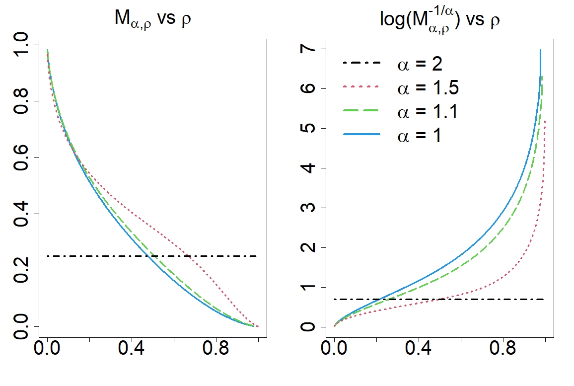
for all 0<t<10<t<1 and δ>0\delta>0. Hence, taking ρ≥1\rho\geq 1 when η=dα\eta=d^{\alpha} for 0<α<20<\alpha<2, as (16) shows, would give Mα,ρ=sup∅=−∞M_{\alpha,\rho}=\sup\emptyset=-\infty. In fact, we find that the derivation of exponential concentration is intractable for xρ,M​Mx_{\rho,MM} with ρ≥1\rho\geq 1 when 1<α<21<\alpha<2, which is why we introduce the new notions of ‘defeat by fraction’ and ‘ρ\rho-geometric-median-of-means estimator’. Fig. 3 demonstrates the shapes of Mα,ρM_{\alpha,\rho} as a function of ρ\rho for several choices of α\alpha. It also depicts Mα,ρ−1/αM_{\alpha,\rho}^{-1/\alpha} on the log scale that appears in the constant factors in the concentration inequalities in the following theorems and corollaries.
Refer to caption
Figure 3: The shapes of Mα,ρM_{\alpha,\rho} (left) and logMα,ρ−1/α\log M_{\alpha,\rho}^{-1/\alpha} (right) as functions of ρ\rho for α=1/1.1/1.5/2\alpha=1/1.1/1.5/2 (solid/dashed/dotted/dot-dashed).
Theorem 6.

Assume (B1) with some constants A,D>0A,D>0 and that there exists a constant Bα>0B_{\alpha}>0 such that

d​(x,x∗)α≤1Bα​∫M(d​(x,y)α−d​(x∗,y)α)​𝑑P​(y).\displaystyle d\left(x,x^{*}\right)^{\alpha}\leq\frac{1}{B_{\alpha}}\int_{M}\left(d(x,y)^{\alpha}-d\left(x^{*},y\right)^{\alpha}\right)\mathrm{d}P(y). (17)

Let ρ∈(0,1)\rho\in(0,1) for α∈(1,2)\alpha\in(1,2) or ρ=1\rho=1 when α=2\alpha=2. Also, let Δ∈(0,1)\Delta\in(0,1) and q∈(0,1/2)q\in(0,1/2). Put Kα=α2​2−2​α+2​Bα−2+2/αK_{\alpha}=\alpha^{2}2^{-2\alpha+2}B_{\alpha}^{-2+2/\alpha}. Let kk denote the number of blocks ℬj\mathcal{B}_{j}. If k=⌈1/(2​q2)​log⁡(1/Δ)⌉k=\lceil 1/(2q^{2})\log(1/\Delta)\rceil, then it holds that, with probability at least 1−Δ1-\Delta, x∗x^{*} defeats by fraction 1/ρ1/\rho all x∈ℳx\in\mathcal{M} with d⁡(x,x∗)>Rq,α,ρd(x,x^{*})>R_{q,\alpha,\rho} but any such xx does not defeat x∗x^{*} by fraction ρ\rho, where

Rq,α,ρ=Cq,α,ρ​σX​log⁡(1/Δ)n,Cq,α,ρ=Mα,ρ−1/α⋅16​2​Kαq(24A​D+21−2​q).\begin{split}&R_{q,\alpha,\rho}=C_{q,\alpha,\rho}\,\sigma_{X}\sqrt{\frac{\log(1/\Delta)}{n}},\\ &C_{q,\alpha,\rho}=M_{\alpha,\rho}^{-1/\alpha}\cdot\frac{16\sqrt{2K_{\alpha}}}{q}\left(24\sqrt{AD}+\frac{2}{\sqrt{1-2q}}\right).\end{split} (18)

Recall that Proposition 2 gives a sufficient condition for the existence of Bα>0B_{\alpha}>0 such that (17) holds. Also, we note that (17) holds with Bα=1B_{\alpha}=1 when α=2\alpha=2, see Section 4.1. Thus, when α=2\alpha=2 and Mα,ρ=1/4M_{\alpha,\rho}=1/4, we have Kα=1K_{\alpha}=1 so that Theorem 6 with ρ=1\rho=1 reduces to Theorem 3. The following corollary may be derived from Theorem 6 as Corollary 1 is from Theorem 3.

Corollary 3.

Assume the conditions and consider the ranges of (ρ,α)(\rho,\alpha), Δ\Delta and qq in Theorem 6. Let kk denote the number of blocks ℬj\mathcal{B}_{j}. If k=⌈1/(2​q2)​log⁡(1/Δ)⌉k=\lceil 1/(2q^{2})\log(1/\Delta)\rceil, then it holds that d⁡(xρ,M​M,x∗)≤Rq,α,ρd(x_{\rho,MM},x^{*})\leq R_{q,\alpha,\rho} with probability at least 1−Δ1-\Delta, where Rq,α,ρR_{q,\alpha,\rho} is the constant defined at (18).

The constant factor Cq,α,ρC_{q,\alpha,\rho} depends on qq and ρ\rho. As in Corollary 1 for xM​Mx_{MM}, it is minimized at some point q∈(0,1/2)q\in(0,1/2). The minimizing qq depends on AA and DD, but is independent of α\alpha and ρ\rho. As for the dependence on ρ\rho, we note that ρ∈(0,1)↦Cq,α,ρ∈(0,+∞)\rho\in(0,1)\mapsto C_{q,\alpha,\rho}\in(0,+\infty) is an increasing function when 1<α<21<\alpha<2, as is well illustrated by the right panel of Fig. 3. The increasing speed gets extremely fast as ρ\rho approaches to 11. Since taking a smaller ρ\rho shrinks the defeating regions Sρ,xS_{\rho,x}, it results in having xρ,M​Mx_{\rho,MM} stay closer to x∗x^{*}, which explains the result that the radius of concentration Rq,α,ρR_{q,\alpha,\rho} gets smaller for smaller ρ\rho.

Below, we present versions of Theorem 6 and Corollary 3 when ℳ\mathcal{M} is of infinite-dimension satisfying the entropy condition (B2). Again, when α=2\alpha=2, we have Kα=1K_{\alpha}=1 and Mα,ρ=1/4M_{\alpha,\rho}=1/4 so that Theorem 7 with ρ=1\rho=1 reduces to Theorem 4.

Theorem 7.

Assume (B2) with some constants A>0A>0 and ζ≥1\zeta\geq 1 and that there exists a constant Bα>0B_{\alpha}>0 such that (17) holds. Consider the ranges of (ρ,α)(\rho,\alpha), Δ\Delta and qq in Theorem 6. Put Kα=α2​2−2​α+2​Bα−2+2/αK_{\alpha}=\alpha^{2}2^{-2\alpha+2}B_{\alpha}^{-2+2/\alpha}. Let kk denote the number of blocks ℬj\mathcal{B}_{j}. If k=⌈1/(2​q2)​log⁡(1/Δ)⌉k=\lceil 1/(2q^{2})\log(1/\Delta)\rceil, then it holds that, with probability at least 1−Δ1-\Delta, x∗x^{*} defeats by fraction 1/ρ1/\rho all x∈ℳx\in\mathcal{M} with d⁡(x,x∗)>Rq,α,ρd(x,x^{*})>R_{q,\alpha,\rho} but any such xx does not defeat x∗x^{*} by fraction ρ\rho, where

Rq,α,ρ,ζ={cq,α,ρ,1⋅log⁡nn1/2⋅σX⋅log⁡1Δif​ζ=1cq,α,ρ,ζ⋅1n1/2​ζ⋅σX⋅(log⁡1Δ)1/2​ζif​ζ>1,cq,α,ρ,ζ=Kα1/2Mα,ρ−1/α⋅CA,ζq​1−2​q\begin{split}R_{q,\alpha,\rho,\zeta}&=\begin{cases}\displaystyle c_{q,\alpha,\rho,1}\cdot\frac{\log n}{n^{1/2}}\cdot\sigma_{X}\cdot\sqrt{\log\frac{1}{\Delta}}\quad&\text{if}\;\;\zeta=1\\ \quad\\ \displaystyle c_{q,\alpha,\rho,\zeta}\cdot\frac{1}{n^{1/2\zeta}}\cdot\sigma_{X}\cdot\left(\log\frac{1}{\Delta}\right)^{1/2\zeta}\quad&\text{if}\;\;\zeta>1,\end{cases}\\[5.69054pt] c_{q,\alpha,\rho,\zeta}&=K_{\alpha}^{1/2}M_{\alpha,\rho}^{-1/\alpha}\cdot\frac{C_{A,\zeta}}{q\sqrt{1-2q}}\end{split} (19)

and CA,ζC_{A,\zeta} is the constant that appears in Theorem 2.

Corollary 4.

Assume the conditions and consider the ranges of (ρ,α)(\rho,\alpha), Δ\Delta and qq in Theorem 7. Let kk denote the number of blocks ℬj\mathcal{B}_{j}. If k=⌈1/(2​q2)​log⁡(1/Δ)⌉k=\lceil 1/(2q^{2})\log(1/\Delta)\rceil, then it holds that d⁡(xρ,M​M,x∗)≤Rq,α,ρ,ζd(x_{\rho,MM},x^{*})\leq R_{q,\alpha,\rho,\zeta} with probability at least 1−Δ1-\Delta, where Rq,α,ρ,ζR_{q,\alpha,\rho,\zeta} is the constant defined at (19).

From (9) and (10) in Section 4.2 we have observed that the concentration rates for the empirical Fréchet mean xnx_{n} in terms of Δ\Delta and nn do not depend on α∈(1,2]\alpha\in(1,2]. This is also the case with the geometric-median-of-means estimators xM​Mx_{MM} and xρ,M​Mx_{\rho,MM}, which can be seen by comparing Corollaries 1 and 2 with Corollaries 3 and 4, respectively. The dependence pattern of the rate of convergence of xρ,M​Mx_{\rho,MM} on the curvature complexity ζ\zeta is the same as xnx_{n} and xM​Mx_{MM}. Also, the dependence of cq,α,ρ,ζc_{q,\alpha,\rho,\zeta} on ρ\rho is the same as in the finite-dimensional case. For the dependence on qq, as in the case of xM​Mx_{MM}, the constant factor is minimized at some point q∈(0,1/2)q\in(0,1/2).

Remark 5.

For NPC spaces ℳ\mathcal{M} with η=d2\eta=d^{2}, the curvature complexity ζ\zeta is greater than or equal to 11 (Proposition 4). However, ζ\zeta may be strictly less than 11 when η=dα\eta=d^{\alpha} with 1<α<21<\alpha<2. In the latter case, one may prove that the radius of concentration Rq,α,ρ,ζR_{q,\alpha,\rho,\zeta} in Theorem 7 is given by

Rq,α,ρ,ζ=cq,α,ρ,ζ⋅1n1/2⋅σX⋅log⁡1Δ,0<ζ<1R_{q,\alpha,\rho,\zeta}=\displaystyle c_{q,\alpha,\rho,\zeta}\cdot\frac{1}{n^{1/2}}\cdot\sigma_{X}\cdot\sqrt{\log\frac{1}{\Delta}},\quad 0<\zeta<1

for the same constant cq,α,ρ,ζc_{q,\alpha,\rho,\zeta} given at (19).

6 Concluding remarks

Our results can be applied to any NPC spaces of finite or infinite dimension, such as Hilbert spaces, hyperbolic spaces, manifolds of SPD matrices, and the Wasserstein space 𝒫2​(ℝ)\mathcal{P}_{2}(\mathbb{R}), etc. Our work is an extensive generalization of previous works on the median-of-means method. It is the first attempt that extends the notion of median-of-means to a general class of metric spaces with a rich class of metrics, and derives exponential concentration for the extended notions of median-of-means in such a general setting. As we discussed in this paper, we stress that the sample Fréchet mean has poor concentration for non-compact or negatively curved spaces. For such spaces, our geometric-median-of-means estimators are efficient antidotes to the sample Fréchet mean.

For Euclidean or Hilbertian spaces ℳ\mathcal{M}, there is a large body of works that study sub-Gaussian mean estimators under only a second moment condition, see [40, 41, 27] and references therein. For general metric spaces, however, the definition of sub-Gaussianity itself is not available. It is a challenging future topic to generalize the notion of sub-Gaussian performance to more general metric spaces and investigate the concentration properties of the corresponding empirical Fréchet means with the extended notion of sub-Gaussianity.

We admit that there is an issue of algorithmic feasibility with the geometric-median-of-means estimator studied in our paper. The computational issue is also present in the Euclidean case for the median-of-means tournament estimator, see [40]. There are some alternative proposals that are equipped with an efficient algorithm. These include the geometric median of [43], Catoni-Giulini estimator of [13], the Hopkins’ estimator [27] and those in the follow-up studies by [15, 17, 36]. However, all these estimators are proposed and studied in the case where ℳ\mathcal{M} is a Euclidean or a Banach space. In particular, the estimators studied in [27, 15, 17, 36] combine the idea of semi-definite programming (SDP) and r-centrality (see [27] for definition), which requires an inner product structure for the underlying space. For some spaces that admit a tangential structure equipped with a bi-invariant metric, one may borrow the idea of Hopkins [27] to find a robust Fréchet mean estimator equipped with an efficient algorithm. For instance, if ℳ=𝒮D+\mathcal{M}=\mathcal{S}_{D}^{+}, the space of symmetric positive-definite matrices, and it is endowed with the log-Euclidean metric, one might project the dataset onto the tangent at the identity IDI_{D} via the logarithmic map, compute the Hopkins’ estimator from the projected data, and then transform the result back to 𝒮D+\mathcal{S}_{D}^{+} via the exponential map. It is straightforward to show that the resulting estimator of the Fréchet mean is consistent. However, this is not an estimator of our interest in this paper, and the special treatment would restrict the study to Riemannian manifolds. It is a challenging topic of study to develop an efficient algorithm for the geometric-median-of-means estimator in the general setting of NPC spaces.

A Proofs of theorems

In the Appendix, we give the complete proofs of Theorems 1–7. The proofs of lemmas and Propositions 1–4 in Section 4, some of which are used in the proofs of Theorems, can be found in the Supplementary Material. Throughout the Appendix and the Supplementary Material, we often denote ∫𝒮f⁡(y)​𝑑Q​(y)\int_{\mathcal{S}}f(y)\,\mathrm{d}Q(y) simply by Q​fQf for a measurable space (𝒮,ℬ)(\mathcal{S},\mathcal{B}), a probability measure QQ on ℬ\mathcal{B} and a measurable function f:𝒮→ℝf:\mathcal{S}\rightarrow\mathbb{R}. For instance, P​f=𝔼⁡(f⁡(X))Pf=\mathbb{E}\,(f(X)) and Pn​f=n−1​∑i=1nf⁡(Xi)P_{n}f=n^{-1}\sum_{i=1}^{n}f(X_{i}). We also suppress the dependence on η\eta of ℳη​(δ)\mathcal{M}_{\eta}(\delta) and other associated terms. All lemmas being referred to by ‘S.xx’ are those in the Supplementary Material.

A.1 Proofs of theorems in Section 3

Define δn=P⁡(η⁡(xn,⋅)−η⁡(x∗,⋅))\delta_{n}=P(\eta(x_{n},\cdot)-\eta\left(x^{*},\cdot\right)) and

ϕn​(δ)\displaystyle\phi_{n}(\delta) =sup{(P−Pn)​(η⁡(x,⋅)−η⁡(x∗,⋅)):x∈ℳ⁡(δ)}\displaystyle=\sup\left\{\left(P-P_{n}\right)\left(\eta(x,\cdot)-\eta\left(x^{*},\cdot\right)\right):x\in\mathcal{M}(\delta)\right\}
=sup{(P−Pn)​(ηc​(x,⋅)−ηc​(x∗,⋅)):x∈ℳ⁡(δ)}\displaystyle=\sup\left\{\left(P-P_{n}\right)\left(\eta_{c}(x,\cdot)-\eta_{c}\left(x^{*},\cdot\right)\right):x\in\mathcal{M}(\delta)\right\}

for δ≥0\delta\geq 0. Since xnx_{n} is a minimizer of Pn​η​(x,⋅)P_{n}\eta(x,\cdot), it follows from the definition of ϕn\phi_{n} that

δn≤(P−Pn)​(η⁡(xn,⋅)−η⁡(x∗,⋅))≤ϕn​(δn).\delta_{n}\leq\left(P-P_{n}\right)\left(\eta\left(x_{n},\cdot\right)-\eta\left(x^{*},\cdot\right)\right)\leq\phi_{n}\left(\delta_{n}\right).

Applying Lemmas S.1 and S.2 we get that, with probability at least 1−(Δ/2)1-(\Delta/2),

ϕn​(δ)≤4​𝔼​ϕn​(δ)+8​2⋅σ¯​(δ)n​Δ.\begin{split}\phi_{n}(\delta)&\leq 4\mathbb{E}\,\phi_{n}(\delta)+\frac{8\sqrt{2}\cdot\bar{\sigma}(\delta)}{\sqrt{n\Delta}}.\end{split} (20)

We first get an upper bound to 𝔼​ϕn​(δ)\mathbb{E}\,\phi_{n}(\delta). Let {εi}\{\varepsilon_{i}\} be a Rademacher sequence, i.e. random signs independent of XiX_{i}’s. Then, by the symmetrization of the associated empirical process (see [26]) we obtain

𝔼​ϕn​(δ)≤2​𝔼​(supx∈ℳ⁡(δ)n−1​∑i=1nεi​(ηc​(x,Xi)−ηc​(x∗,Xi)))=2​𝔼​(supx∈ℳ⁡(δ)n−1​∑i=1nεi​ηc​(x,Xi)).\begin{split}\mathbb{E}\,\phi_{n}(\delta)&\leq 2\,\mathbb{E}\,\bigg(\sup_{x\in\mathcal{M}(\delta)}n^{-1}\sum_{i=1}^{n}\varepsilon_{i}\left(\eta_{c}(x,X_{i})-\eta_{c}(x^{*},X_{i})\right)\bigg)\\ &=2\,\mathbb{E}\,\bigg(\sup_{x\in\mathcal{M}(\delta)}n^{-1}\sum_{i=1}^{n}\varepsilon_{i}\,\eta_{c}(x,X_{i})\bigg).\end{split}

One can easily check that the Rademacher empirical process {Yf:f∈(ℱ(δ),∥⋅∥2,Pn)}\{Y_{f}:f\in(\mathcal{F}(\delta),\|\cdot\|_{2,P_{n}})\} for the pseudo metric space (ℱ(δ),∥⋅∥2,Pn)(\mathcal{F}(\delta),\|\cdot\|_{2,P_{n}}) given by

Yf:=1n​∑i=1nεi​f​(Xi)Y_{f}:=\frac{1}{\sqrt{n}}\sum_{i=1}^{n}\varepsilon_{i}f(X_{i})

is n\sqrt{n}-Lipschitz with respect to ∥⋅∥2,Pn\|\cdot\|_{2,P_{n}}, conditionally on the XiX_{i}’s. It is also sub-Gaussian. To see this, we note that, for any a1,…,an∈ℝa_{1},\dots,a_{n}\in\mathbb{R},

𝔼⁡(exp⁡(∑i=1nai​εi))=∏i=1n𝔼​eai​εi=∏i=1neai+e−ai2≤∏i=1neai2/2=exp⁡(∑i=1nai22),\displaystyle\mathbb{E}\bigg(\exp\Big(\sum_{i=1}^{n}a_{i}\varepsilon_{i}\Big)\bigg)=\prod_{i=1}^{n}\mathbb{E}e^{a_{i}\varepsilon_{i}}=\prod_{i=1}^{n}\frac{e^{a_{i}}+e^{-a_{i}}}{2}\leq\prod_{i=1}^{n}e^{a_{i}^{2}/2}=\exp\Big(\sum_{i=1}^{n}\frac{a_{i}^{2}}{2}\Big),

where the inequality follows from Taylor’s expansion. From this we get that, for any f,g∈ℱ⁡(δ)f,g\in\mathcal{F}(\delta) and θ∈ℝ\theta\in\mathbb{R},

𝔼⁡(eθ⁡(Yf−Yg)|X1,…,Xn)\displaystyle\mathbb{E}\big(e^{\theta\left(Y_{f}-Y_{g}\right)}|X_{1},\dots,X_{n}\big) =𝔼⁡(exp⁡(θn​∑i=1nεi​(f−g)​(Xi))|X1,…,Xn)\displaystyle=\mathbb{E}\bigg(\exp\Big(\frac{\theta}{\sqrt{n}}\sum_{i=1}^{n}\varepsilon_{i}(f-g)(X_{i})\Big)\Big|X_{1},\dots,X_{n}\bigg)
≤exp⁡(θ22​n​∑i=1n(f⁡(Xi)−g⁡(Xi))2)\displaystyle\leq\exp\bigg(\frac{\theta^{2}}{2n}\sum_{i=1}^{n}(f(X_{i})-g(X_{i}))^{2}\bigg)
=exp⁡(θ22​‖f−g‖2,Pn2).\displaystyle=\exp\Big(\frac{\theta^{2}}{2}\|f-g\|_{2,P_{n}}^{2}\Big).

Thus, YfY_{f} satisfies the conditions of Lemma S.3 (see [2]). Applying Lemma S.3 with (B1) and using the inequalities for HδH_{\delta} given in Lemma S.2, we get

𝔼​ϕn​(δ)≤2​𝔼​infε≥0(2​ε+12n​∫ε∞logN(u,ℱ(δ),∥⋅∥2,Pn)​du)≤2​𝔼​infε≥0(2​ε+12n​∫ε‖Hδ‖2,PnD​log⁡(A​‖Hδ‖2,Pnu)​du)=2​𝔼​(‖Hδ‖2,Pn)⋅infε′≥0(2​ε′+12n​∫ε′1D​log⁡(Au)​du)≤48​𝔼​(‖Hδ‖2,Pn)⋅A​Dn≤48​σ¯​(δ)​A​Dn,\begin{split}\mathbb{E}\,\phi_{n}(\delta)&\leq 2\,\mathbb{E}\,\inf_{\varepsilon\geq 0}\left(2\varepsilon+\frac{12}{\sqrt{n}}\int_{\varepsilon}^{\infty}\sqrt{\log N(u,\mathcal{F}(\delta),\|\cdot\|_{2,P_{n}})}\mathrm{d}u\right)\\ &\leq 2\,\mathbb{E}\,\inf_{\varepsilon\geq 0}\left(2\varepsilon+\frac{12}{\sqrt{n}}\int_{\varepsilon}^{\|H_{\delta}\|_{2,P_{n}}}\sqrt{D\log\left(\frac{A\|H_{\delta}\|_{2,P_{n}}}{u}\right)}\,\mathrm{d}u\right)\\ &=2\,\mathbb{E}\left(\|H_{\delta}\|_{2,P_{n}}\right)\cdot\inf_{\varepsilon^{\prime}\geq 0}\,\left(2\varepsilon^{\prime}+\frac{12}{\sqrt{n}}\int_{\varepsilon^{\prime}}^{1}\sqrt{D\log\left(\frac{A}{u}\right)}\,\mathrm{d}u\right)\\ &\leq 48\,\mathbb{E}\left(\|H_{\delta}\|_{2,P_{n}}\right)\cdot\sqrt{\frac{AD}{n}}\\ &\leq 48\,\bar{\sigma}(\delta)\sqrt{\frac{AD}{n}},\end{split} (21)

where in the third inequality we have used log⁡x≤x−1≤x\log x\leq x-1\leq x for x>0x>0.

The inequalities (20) and (21) imply that, with probability at least 1−(Δ/2)1-(\Delta/2),

ϕn​(δ)≤σ¯​(δ)​(192​A​Dn+8​2n​Δ)≤32​K​σX2​δβn​(24​A​D+2Δ)=:bn​(δ,Δ).\begin{split}\phi_{n}(\delta)&\leq\bar{\sigma}(\delta)\left(192\sqrt{\frac{AD}{n}}+\frac{8\sqrt{2}}{\sqrt{n\Delta}}\right)\\ &\leq 32\sqrt{\frac{K\sigma_{X}^{2}\delta^{\beta}}{n}}\left(24\sqrt{AD}+\sqrt{\frac{2}{\Delta}}\right)\\ &=:b_{n}(\delta,\Delta).\end{split}

Since ϕn​(δ)\phi_{n}(\delta) is an increasing function and bn​(δ,Δ)b_{n}(\delta,\Delta) is decreasing in Δ\Delta for fixed δ\delta, it follows from Theorem 4.3 in [31] that

δn≤ϕn​(δn)≤bn​(Δ):=inf{τ>0:supδ≥τδ−1​bn​(δ,Δδτ)≤1}\delta_{n}\leq\phi_{n}(\delta_{n})\leq b_{n}(\Delta):=\inf\left\{\tau>0:\sup_{\delta\geq\tau}\delta^{-1}b_{n}\left(\delta,\Delta^{\frac{\delta}{\tau}}\right)\leq 1\right\} (22)

with probability at least 1−Δ1-\Delta. Since σ¯​(δ)/δ\bar{\sigma}(\delta)/\delta is decreasing in δ\delta as β∈(0,2)\beta\in(0,2),

supδ≥τδ−1​bn​(δ,Δδτ)=bn​(τ,Δ)τ=32​K​σX2​τ−(2−β)n​(24​A​D+2Δ).\sup_{\delta\geq\tau}\delta^{-1}b_{n}\left(\delta,\Delta^{\frac{\delta}{\tau}}\right)=\frac{b_{n}(\tau,\Delta)}{\tau}=32\sqrt{\frac{K\sigma_{X}^{2}\tau^{-(2-\beta)}}{n}}\left(24\sqrt{AD}+\sqrt{\frac{2}{\Delta}}\right).

This gives

bn​(Δ)\displaystyle b_{n}(\Delta) =inf{τ>0:32​K​σX2​τ−(2−β)n​(24​A​D+2Δ)≤1}\displaystyle=\inf\left\{\tau>0:32\sqrt{\frac{K\sigma_{X}^{2}\tau^{-(2-\beta)}}{n}}\left(24\sqrt{AD}+\sqrt{\frac{2}{\Delta}}\right)\leq 1\right\} (23)
={32​K​σX2n​(24​A​D+2Δ)}22−β.\displaystyle=\left\{32\sqrt{\frac{K\sigma_{X}^{2}}{n}}\left(24\sqrt{AD}+\sqrt{\frac{2}{\Delta}}\right)\right\}^{\frac{2}{2-\beta}}.

Applying (23) to (22), we obtain that, with probability at least 1−Δ1-\Delta,

l⁡(xn,x∗)\displaystyle l(x_{n},x^{*}) ≤K⋅δnβ/2\displaystyle\leq\sqrt{K}\cdot\delta_{n}^{\beta/2}
≤K12−β​{32​(24​A​D+2Δ)​σXn}β2−β.\displaystyle\leq K^{\frac{1}{2-\beta}}\left\{32\left(24\sqrt{AD}+\sqrt{\frac{2}{\Delta}}\right)\frac{\sigma_{X}}{\sqrt{n}}\right\}^{\frac{\beta}{2-\beta}}.

This completes the proof of Theorem 1. ∎

The proof is similar to that of Theorem 1 for the case of finite-dimensional ℳ\mathcal{M}. The difference is in the covering number N(u,ℱ(δ),∥⋅∥2,Pn)N(u,\mathcal{F}(\delta),\|\cdot\|_{2,P_{n}}). We get

𝔼​ϕn​(δ)\displaystyle\mathbb{E}\,\phi_{n}(\delta) ≤2​𝔼​infε≥0(2​ε+12n​∫ε‖Hδ‖2,PnA​‖Hδ‖2,Pn2​ζu2​ζ​𝑑u)\displaystyle\leq 2\,\mathbb{E}\,\inf_{\varepsilon\geq 0}\left(2\varepsilon+\frac{12}{\sqrt{n}}\int_{\varepsilon}^{\|H_{\delta}\|_{2,P_{n}}}\sqrt{\frac{A\|H_{\delta}\|_{2,P_{n}}^{2\zeta}}{u^{2\zeta}}}\,\mathrm{d}u\right)
=4​𝔼​(‖Hδ‖2,Pn)⋅infε≥0(ε+6​An​∫ε1u−ζ​𝑑u)\displaystyle=4\,\mathbb{E}\,\left(\|H_{\delta}\|_{2,P_{n}}\right)\cdot\inf_{\varepsilon\geq 0}\,\left(\varepsilon+6\sqrt{\frac{A}{n}}\int_{\varepsilon}^{1}u^{-\zeta}\,\mathrm{d}u\right)
≤4​𝔼​(‖Hδ‖2,Pn)×{61−ζ​Anif ​0<ζ<16​An​(1−log⁡(6​An))if ​ζ=1ζζ−1​(6​An)1/ζif ​ζ>1..\displaystyle\leq 4\,\mathbb{E}\,\left(\|H_{\delta}\|_{2,P_{n}}\right)\times\begin{cases}\displaystyle\frac{6}{1-\zeta}\sqrt{\frac{A}{n}}\quad&\text{if }0<\zeta<1\\[11.38109pt] \displaystyle 6\sqrt{\frac{A}{n}}\left(1-\log\Big(6\sqrt{\frac{A}{n}}\Big)\right)\quad&\text{if }\zeta=1\\[5.69054pt] \displaystyle\frac{\zeta}{\zeta-1}\left(6\sqrt{\frac{A}{n}}\right)^{1/\zeta}\quad&\text{if }\zeta>1.\end{cases}.

Therefore, ϕn​(δn)≤bn​(Δ)\phi_{n}(\delta_{n})\leq b_{n}(\Delta) with probability at least 1−Δ1-\Delta, now with

bn​(Δ)={(32​K​σX2​(121−ζ​An+2n​Δ))22−βif ​0<ζ<1(32​K​σX2​(12​An​(1−log⁡(6​An))+2n​Δ))22−βif ​ζ=1(32​K​σX2​(2​ζζ−1​(6​An)1/ζ+2n​Δ))22−βif ​ζ>1.\displaystyle b_{n}(\Delta)=\begin{cases}\displaystyle\left(32\sqrt{K\sigma_{X}^{2}}\left(\frac{12}{1-\zeta}\sqrt{\frac{A}{n}}+\sqrt{\frac{2}{n\Delta}}\right)\right)^{\frac{2}{2-\beta}}\quad&\text{if }0<\zeta<1\\ \displaystyle\left(32\sqrt{K\sigma_{X}^{2}}\left(12\sqrt{\frac{A}{n}}\left(1-\log\left(6\sqrt{\frac{A}{n}}\right)\right)+\sqrt{\frac{2}{n\Delta}}\right)\right)^{\frac{2}{2-\beta}}\quad&\text{if }\zeta=1\\ \displaystyle\left(32\sqrt{K\sigma_{X}^{2}}\left(\frac{2\zeta}{\zeta-1}\left(6\sqrt{\frac{A}{n}}\right)^{1/\zeta}+\sqrt{\frac{2}{n\Delta}}\right)\right)^{\frac{2}{2-\beta}}\quad&\text{if }\zeta>1.\end{cases}

This gives the theorem. ∎

A.2 Proofs of theorems in Section 5

Without loss of generality, we assume that n=m⋅kn=m\cdot k, where kk is the number of blocks in splitting the sample and mm is the size of each block.

Let F⁡(x)=∫ℳη⁡(x,y)​𝑑P​(y)F(x)=\int_{\mathcal{M}}\eta(x,y)\,\mathrm{d}P(y). By the definition of x∗x^{*} it holds that, for each block ℬj\mathcal{B}_{j},

Fn,j​(x∗)−Fn,j​(Zj)≤Fn,j​(x∗)−Fn,j​(Zj)−F⁡(x∗)+F⁡(Zj).F_{n,j}(x^{*})-F_{n,j}(Z_{j})\leq F_{n,j}(x^{*})-F_{n,j}(Z_{j})-F(x^{*})+F(Z_{j}).

The right hand side has an upper bound that is analogous to ϕn​(δn)\phi_{n}(\delta_{n}) in the proof of Theorem 1, which is obtained by substituting the empirical measure corresponding to ℬj\mathcal{B}_{j} for PnP_{n} and ZjZ_{j} for xnx_{n}. Thus, replacing Δ\Delta by (1−2​q)/2(1-2q)/2 (so that 1−Δ1-\Delta by q+1/2q+1/2) and nn by m=n/km=n/k with K=β=1K=\beta=1, we get from (22) and (23) that

ℙ⁡(Fn,j​(x∗)−Fn,j​(Zj)≤εq2)≥q+12,\mathbb{P}\left(F_{n,j}(x^{*})-F_{n,j}(Z_{j})\leq\varepsilon_{q}^{2}\right)\geq q+\frac{1}{2}, (24)

where

εq=32​k​σX2n​(24​A​D+21−2​q).\displaystyle\varepsilon_{q}=32\sqrt{\frac{k\sigma_{X}^{2}}{n}}\left(24\sqrt{AD}+\frac{2}{\sqrt{1-2q}}\right). (25)

By the CN inequality in Section 4.1, we have

Fn,j​(Zj)≤Fn,j​(γ1/2x)≤Fn,j​(x)2+Fn,j​(x∗)2−d​(x∗,x)24⇔Fn,j​(x)−Fn,j​(Zj)≥−(Fn,j​(x∗)−Fn,j​(Zj))+d​(x∗,x)22,\begin{split}&F_{n,j}(Z_{j})\leq F_{n,j}(\gamma_{1/2}^{x})\leq\frac{F_{n,j}(x)}{2}+\frac{F_{n,j}(x^{*})}{2}-\frac{d(x^{*},x)^{2}}{4}\\ \Leftrightarrow\;&F_{n,j}(x)-F_{n,j}(Z_{j})\geq-\left(F_{n,j}(x^{*})-F_{n,j}(Z_{j})\right)+\frac{d(x^{*},x)^{2}}{2},\end{split}

where γx:[0,1]→ℳ\gamma^{x}:[0,1]\to\mathcal{M} is the geodesic with γ0x=x∗\gamma_{0}^{x}=x^{*} and γ1x=x\gamma_{1}^{x}=x. Thus, denoting by ℰn,j\mathcal{E}_{n,j} the event

Fn,j​(x)>Fn,j​(x∗)for all ​x∈ℳ​ with ​d​(x,x∗)>2​εq,F_{n,j}(x)>F_{n,j}(x^{*})\quad\mbox{for all }\,x\in\mathcal{M}\mbox{ with }d(x,x^{*})>2\varepsilon_{q},

we get from (24) that ℙ⁡(ℰn,j)≥q+1/2\mathbb{P}\,(\mathcal{E}_{n,j})\geq q+1/2 since Fn,j​(x∗)−Fn,j​(Zj)≤εq2F_{n,j}(x^{*})-F_{n,j}(Z_{j})\leq\varepsilon_{q}^{2} implies

Fn,j​(x)−Fn,j​(Zj)>−(Fn,j​(x∗)−Fn,j​(Zj))+2​εq2≥Fn,j​(x∗)−Fn,j​(Zj)F_{n,j}(x)-F_{n,j}(Z_{j})>-\left(F_{n,j}(x^{*})-F_{n,j}(Z_{j})\right)+2\varepsilon_{q}^{2}\;\geq\;F_{n,j}(x^{*})-F_{n,j}(Z_{j})

for all xx with d⁡(x,x∗)>2​εqd(x,x^{*})>2\varepsilon_{q}. By applying Høffding’s inequality to ∑j=1kI⁡(ℰn,j)\sum_{j=1}^{k}I(\mathcal{E}_{n,j}), we obtain

1−Δ\displaystyle 1-\Delta ≤1−e−2​q2​k\displaystyle\leq 1-e^{-2q^{2}k}
≤ℙ⁡(∑j=1kI⁡(ℰn,j)>k/2)\displaystyle\leq\mathbb{P}\left(\sum_{j=1}^{k}I(\mathcal{E}_{n,j})>k/2\right)
≤ℙ⁡(∑j=1kI⁡(Fn,j​(x)>Fn,j​(x∗))>k/2​ for all ​x∈ℳ​ with ​d​(x,x∗)>2​εq).\displaystyle\leq\mathbb{P}\left(\sum_{j=1}^{k}I\left(F_{n,j}(x)>F_{n,j}(x^{*})\right)>k/2\;\mbox{ for all }x\in\mathcal{M}\text{ with }d(x,x^{*})>2\varepsilon_{q}\right).

This completes the proof of the theorem. ∎

The proof is essentially the same as that of Theorem 3 except that we use Theorem 2 instead of Theorem 1. We obtain (24) now with

εq,ζ={CA,1⋅log⁡(n/k)n/k⋅σX(1−2​q)/2,if​ζ=1CA,ζ⋅(k/n)1/2​ζ⋅σX(1−2​q)/2,if​ζ>1.\displaystyle\varepsilon_{q,\zeta}=\begin{cases}\displaystyle C_{A,1}\cdot\frac{\log(n/k)}{\sqrt{n/k}}\cdot\frac{\sigma_{X}}{\sqrt{(1-2q)/2}},&\text{if}\;\;\zeta=1\\ \quad\\ \displaystyle C_{A,\zeta}\cdot(k/n)^{1/2\zeta}\cdot\frac{\sigma_{X}}{\sqrt{(1-2q)/2}},&\text{if}\;\;\zeta>1.\end{cases} (26)

Since

12​q​log⁡n​log⁡(1/Δ)n=k​log⁡nn≥log⁡(n/k)n/k,12​qn−1/2ζ(log1Δ)1/2​ζ≥(2​q2​nlog⁡(1/Δ))−1/2ζ=(k/n)1/2​ζ,\begin{split}&\frac{1}{\sqrt{2}q}\frac{\log n\sqrt{\log(1/\Delta)}}{\sqrt{n}}=\frac{\sqrt{k}\log n}{\sqrt{n}}\geq\frac{\log(n/k)}{\sqrt{n/k}},\\ &\frac{1}{\sqrt{2}q}n^{-1/2\zeta}\left(\log\frac{1}{\Delta}\right)^{1/2\zeta}\geq\left(\frac{2q^{2}n}{\log(1/\Delta)}\right)^{-1/2\zeta}=(k/n)^{1/2\zeta},\end{split} (27)

we get εq,ζ≤Rq,ζ/2\varepsilon_{q,\zeta}\leq R_{q,\zeta}/2. The rest of the proof is the same as in the proof of Theorem 3. ∎

Fix a partition {ℬj:1≤j≤k}\{\mathcal{B}_{j}:1\leq j\leq k\} of the original dataset 𝒳n={X1,…,Xn}\mathcal{X}_{n}=\{X_{1},\ldots,X_{n}\}. Let ℬj={X1,j,…,Xm,j}\mathcal{B}_{j}=\{X_{1,j},\ldots,X_{m,j}\} for 1≤j≤k1\leq j\leq k. Choose a point O∈ℳO\in\mathcal{M} and let DO=max1≤i≤n⁡d⁡(O,Xi)D_{O}=\max_{1\leq i\leq n}d(O,X_{i}). We let X~i\tilde{X}_{i} denote a corrupted value corresponding to XiX_{i}, and we write A~\tilde{A} instead of AA if a term AA involves corrupted values. For example, we write F~n,j​(x)\tilde{F}_{n,j}(x) instead of Fn,j​(x)F_{n,j}(x) when the jjth block contains a corrupted value. In particular, we write in this proof S~x\tilde{S}_{x} and r~x\tilde{r}_{x} for each point x∈ℳx\in\mathcal{M} rather than SxS_{x} and rxr_{x}, respectively, since the defeating region and radius always depend on corrupted values. Put L:=⌈(k+1)/2⌉L:=\lceil(k+1)/2\rceil.

We first show that εn∗≤L/n\varepsilon_{n}^{*}\leq L/n by contradiction. Suppose that it is false, i.e., εn∗>L/n\varepsilon_{n}^{*}>L/n. Then, for an arbitrary configuration {j⁡(1),…,j⁡(L)}⊂{1,2,…,k}\{j(1),\ldots,j(L)\}\subset\{1,2,\ldots,k\} with the corruption X~1,1=X~1,2=⋯=X~1,L=x~\tilde{X}_{1,1}=\tilde{X}_{1,2}=\dots=\tilde{X}_{1,L}=\tilde{x}, there exists R>0R>0 such that supx~∈ℳd⁡(O,x~M​M)<R\sup_{\tilde{x}\in\mathcal{M}}d(O,\tilde{x}_{MM})<R. We may assume R>m−1⋅DOR>\sqrt{m-1}\cdot D_{O}. Now, let γ~:[0,1]→ℳ\tilde{\gamma}:[0,1]\rightarrow\mathcal{M} be the geodesic connecting γ~0=O\tilde{\gamma}_{0}=O and γ~1=x~\tilde{\gamma}_{1}=\tilde{x} with the length D~:=d⁡(x~,O)\tilde{D}:=d(\tilde{x},O) larger than RR. For j=1,…,Lj=1,\dots,L, by the triangular inequality,

m⋅(F~n,j​(x~M​M)−F~n,j​(γ~t))\displaystyle m\cdot(\tilde{F}_{n,j}(\tilde{x}_{MM})-\tilde{F}_{n,j}(\tilde{\gamma}_{t})) ≥d​(x~,x~M​M)2−(1−t)2​D~2−∑i=2md​(γ~t,Xi​j)2\displaystyle\geq d(\tilde{x},\tilde{x}_{MM})^{2}-(1-t)^{2}\tilde{D}^{2}-\sum_{i=2}^{m}d(\tilde{\gamma}_{t},X_{ij})^{2}
≥(D~−R)2−(1−t)2​D~2−(m−1)​(t​D~+DO)2\displaystyle\geq(\tilde{D}-R)^{2}-(1-t)^{2}\tilde{D}^{2}-(m-1)(t\tilde{D}+D_{O})^{2}
=(2​t−m​t2)​D~2−2​(R+DO​(m−1)​t)​D~+(R2−(m−1)⋅DO2)\displaystyle=(2t-mt^{2})\tilde{D}^{2}-2(R+D_{O}(m-1)t)\tilde{D}+(R^{2}-(m-1)\cdot D_{O}^{2})
≥(2​t−m​t2)​D~2−2​(R+DO​(m−1)​t)​D~.\displaystyle\geq(2t-mt^{2})\tilde{D}^{2}-2(R+D_{O}(m-1)t)\tilde{D}.

This implies that for all t<2/mt<2/m, the point γ~t\tilde{\gamma}_{t} defeats x~M​M\tilde{x}_{MM} whenever

D~≥2​(R+DO​(m−1)​t)2​t−m​t2,\tilde{D}\geq\frac{2(R+D_{O}(m-1)t)}{2t-mt^{2}},

so the defeating radius of x~M​M\tilde{x}_{MM} satisfies r~x~M​M≥d⁡(γ~t,x~M​M)\tilde{r}_{\tilde{x}_{MM}}\geq d(\tilde{\gamma}_{t},\tilde{x}_{MM}). Therefore,

lim infD~→∞r~x~M​MD~≥lim infD~→∞sup0<t<2/md⁡(γ~t,x~M​M)D~=lim infD~→∞sup0<t<2/md⁡(γ~t,O)D~=2m.\liminf_{\tilde{D}\rightarrow\infty}\frac{\tilde{r}_{\tilde{x}_{MM}}}{\tilde{D}}\geq\liminf_{\tilde{D}\rightarrow\infty}\sup_{0<t<2/m}\frac{d(\tilde{\gamma}_{t},\tilde{x}_{MM})}{\tilde{D}}=\liminf_{\tilde{D}\rightarrow\infty}\sup_{0<t<2/m}\frac{d(\tilde{\gamma}_{t},O)}{\tilde{D}}=\frac{2}{m}. (28)

Now, choose any x∈S~γ~1/m(≠∅)x\in\tilde{S}_{\tilde{\gamma}_{1/m}}(\neq\emptyset), i.e. xx defeating γ~1/m\tilde{\gamma}_{1/m}. Then, ∃\exists at least one j0∈{j⁡(1),…,j⁡(L)}j_{0}\in\{j(1),\ldots,j(L)\} such that F~n,j0​(x)≤F~n,j0​(γ~1/m)\tilde{F}_{n,j_{0}}(x)\leq\tilde{F}_{n,j_{0}}(\tilde{\gamma}_{1/m}). Due to the CN inequality,

0\displaystyle 0 ≤m⋅(F~n,j0​(γ~1/m)−F~n,j0​(x))\displaystyle\leq m\cdot(\tilde{F}_{n,j_{0}}(\tilde{\gamma}_{1/m})-\tilde{F}_{n,j_{0}}(x)) (29)
=d​(γ~1/m,x~)2−d​(x,x~)2+∑i=2m(d​(γ~1/m,Xi,j0)2−d​(x,Xi,j0)2)\displaystyle=d(\tilde{\gamma}_{1/m},\tilde{x})^{2}-d(x,\tilde{x})^{2}+\sum_{i=2}^{m}\left(d(\tilde{\gamma}_{1/m},X_{i,j_{0}})^{2}-d(x,X_{i,j_{0}})^{2}\right)
≤(m−1m)2​D~2−d​(x,x~)2\displaystyle\leq\left(\frac{m-1}{m}\right)^{2}\tilde{D}^{2}-d(x,\tilde{x})^{2}
+∑i=2m{m−1md(O,Xi,j0)2+1md(x~,Xi,j0)2−m−1m2D~2−d(x,Xi,j0)2}.\displaystyle\qquad+\sum_{i=2}^{m}\left\{\frac{m-1}{m}d(O,X_{i,j_{0}})^{2}+\frac{1}{m}d(\tilde{x},X_{i,j_{0}})^{2}-\frac{m-1}{m^{2}}\tilde{D}^{2}-d(x,X_{i,j_{0}})^{2}\right\}.

Note that again by the CN inequality,

d​(x,γ~1/m)2≤m−1m​d​(O,x)2+1m​d​(x,x~)2−m−1m2​D~2.d(x,\tilde{\gamma}_{1/m})^{2}\leq\frac{m-1}{m}d(O,x)^{2}+\frac{1}{m}d(x,\tilde{x})^{2}-\frac{m-1}{m^{2}}\tilde{D}^{2}.

Plugging this inequality into (29) and using the triangular inequality, we get

0\displaystyle 0 ≤m−1m2​D~2−m⋅d​(x,γ~1/m)2\displaystyle\leq\frac{m-1}{m^{2}}\tilde{D}^{2}-m\cdot d(x,\tilde{\gamma}_{1/m})^{2}
+∑i=2m{m−1md(O,Xi,j0)2+1md(x~,Xi,j0)2−m−1m2D~2+d(O,x)2−d(x,Xi,j0)2}\displaystyle\quad+\sum_{i=2}^{m}\left\{\frac{m-1}{m}d(O,X_{i,j_{0}})^{2}+\frac{1}{m}d(\tilde{x},X_{i,j_{0}})^{2}-\frac{m-1}{m^{2}}\tilde{D}^{2}+d(O,x)^{2}-d(x,X_{i,j_{0}})^{2}\right\}
≤m−1m2​D~2−m⋅d​(x,γ~1/m)2\displaystyle\leq\frac{m-1}{m^{2}}\tilde{D}^{2}-m\cdot d(x,\tilde{\gamma}_{1/m})^{2}
+(m−1)​{m−1m​DO2+1m​(D~+DO)2−m−1m2​D~2+2​DO⋅d⁡(O,x)−DO2}\displaystyle\quad+(m-1)\left\{\frac{m-1}{m}D_{O}^{2}+\frac{1}{m}(\tilde{D}+D_{O})^{2}-\frac{m-1}{m^{2}}\tilde{D}^{2}+2D_{O}\cdot d(O,x)-D_{O}^{2}\right\}
≤m−1m2​D~2−m⋅d​(x,γ~1/m)2\displaystyle\leq\frac{m-1}{m^{2}}\tilde{D}^{2}-m\cdot d(x,\tilde{\gamma}_{1/m})^{2}
+(m−1)​{m−1m​DO2+1m​(D~+DO)2−m−1m2​D~2+2​DO​(D~m+d⁡(x,γ~1/m))−DO2}\displaystyle\quad+(m-1)\left\{\frac{m-1}{m}D_{O}^{2}+\frac{1}{m}(\tilde{D}+D_{O})^{2}-\frac{m-1}{m^{2}}\tilde{D}^{2}+2D_{O}\left(\frac{\tilde{D}}{m}+d(x,\tilde{\gamma}_{1/m})\right)-D_{O}^{2}\right\}
=−m⋅d(x,γ~1/m)2+2(m−1)DO⋅d(x,γ~1/m)+2​(m−1)​D~​(D~+2​m​DO)m2.\displaystyle=-m\cdot d(x,\tilde{\gamma}_{1/m})^{2}+2(m-1)D_{O}\cdot d(x,\tilde{\gamma}_{1/m})+\frac{2(m-1)\tilde{D}(\tilde{D}+2mD_{O})}{m^{2}}.

Therefore,

d⁡(x,γ~1/m)≤m⁡(m−1)​DO+m2​(m−1)2​DO2+2​m​(m−1)​D~​(D~+2​m​DO)m2.\displaystyle d(x,\tilde{\gamma}_{1/m})\leq\frac{m(m-1)D_{O}+\sqrt{m^{2}(m-1)^{2}D_{O}^{2}+2m(m-1)\tilde{D}(\tilde{D}+2mD_{O})}}{m^{2}}.

Since x∈S~γ~1/mx\in\tilde{S}_{\tilde{\gamma}_{1/m}} was chosen arbitrarily, we have

lim supD~→∞r~γ~1/mD~\displaystyle\limsup_{\tilde{D}\rightarrow\infty}\frac{\tilde{r}_{\tilde{\gamma}_{1/m}}}{\tilde{D}} ≤lim supD~→∞m⁡(m−1)​DO+m2​(m−1)2​DO2+2​m​(m−1)​D~​(D~+2​m​DO)m2​D~\displaystyle\leq\limsup_{\tilde{D}\rightarrow\infty}\frac{m(m-1)D_{O}+\sqrt{m^{2}(m-1)^{2}D_{O}^{2}+2m(m-1)\tilde{D}(\tilde{D}+2mD_{O})}}{m^{2}\tilde{D}}
=2m\displaystyle=\frac{\sqrt{2}}{m}
<2m.\displaystyle<\frac{2}{m}.

In view of (28), the above strict inequality is contradictory to the fact that r~x~M​M≤r~γ~1/m\tilde{r}_{\tilde{x}_{MM}}\leq\tilde{r}_{\tilde{\gamma}_{1/m}} for all D~\tilde{D} from the definition of geometric-median-of-means.

Next, we show that

sup∗​d​(O,x~M​M)<∞,\mbox{$\sup_{*}$}d(O,\tilde{x}_{MM})<\infty, (30)

where sup∗\sup_{*} denotes the supremum over all configurations of s≤(L−1)s\leq(L-1) arbitrary corruptions among {X1,…,Xn}\{X_{1},\ldots,X_{n}\}. We note that (30) implies εn∗≥L/n\varepsilon_{n}^{*}\geq L/n. To prove (30), let s≤L−1s\leq L-1 be the number of corrupted X~i\tilde{X}_{i} and think of a configuration of the indices of X~i\tilde{X}_{i}, say {i⁡(1),…,i⁡(s)}⊂{1,2,…,n}\{i(1),\ldots,i(s)\}\subset\{1,2,\ldots,n\}. The corrupted X~i⁡(1),…,X~i⁡(s)\tilde{X}_{i(1)},\ldots,\tilde{X}_{i(s)} are scattered across the kk blocks ℬj, 1≤j≤k\mathcal{B}_{j},\,1\leq j\leq k. Without loss of generality, let ℬ1,…,ℬJ\mathcal{B}_{1},\ldots,\mathcal{B}_{J} denote those blocks that do not contain any of the corrupted values. We note that J>k/2J>k/2 since s≤L−1s\leq L-1. We claim

supX~i⁡(1),…,X~i⁡(s)max1≤j≤J⁡r~Zj<∞.\sup_{\tilde{X}_{i(1)},\ldots,\tilde{X}_{i(s)}}\max_{1\leq j\leq J}\tilde{r}_{Z_{j}}<\infty. (31)

Then, by the definition of the geometric-median-of-means we get

supX~i⁡(1),…,X~i⁡(s)r~x~M​M<∞.\sup_{\tilde{X}_{i(1)},\ldots,\tilde{X}_{i(s)}}\tilde{r}_{\tilde{x}_{MM}}<\infty. (32)

Also, by the definition of xx-defeating radius and since J>k/2J>k/2, it holds that

r~x≥radx​(⋂j=1J{y∈ℳ:Fn,j​(y)≤Fn,j​(x)})≥radx​(⋂j=1k{y∈ℳ:Fn,j​(y)≤Fn,j​(x)})\displaystyle\begin{split}\tilde{r}_{x}&\geq{\rm rad}_{x}\left(\bigcap_{j=1}^{J}\{y\in\mathcal{M}:F_{n,j}(y)\leq F_{n,j}(x)\}\right)\\ &\geq{\rm rad}_{x}\left(\bigcap_{j=1}^{k}\{y\in\mathcal{M}:F_{n,j}(y)\leq F_{n,j}(x)\}\right)\end{split} (33)

for all x∈ℳx\in\mathcal{M}, where radx​(A){\rm rad}_{x}(A) stands for the radius of the smallest ball centered at xx that covers AA. The right hand side of the second inequality in (33) depends solely on the original dataset {X1,…,Xn}\{X_{1},\ldots,X_{n}\}, independent of data corruption. Now, suppose that there exists s≤L−1s\leq L-1 and a configuration {i⁡(1),…,i⁡(s)}\{i(1),\ldots,i(s)\} such that

supX~i⁡(1),…,X~i⁡(s)d⁡(O,x~M​M)=∞.\sup_{\tilde{X}_{i(1)},\ldots,\tilde{X}_{i(s)}}d(O,\tilde{x}_{MM})=\infty.

Then, since the right hand side of the second inequality in (33) diverges to infinity as d⁡(O,x)→∞d(O,x)\rightarrow\infty, we would obtain

supX~i⁡(1),…,X~i⁡(s)r~x~M​M=∞,\sup_{\tilde{X}_{i(1)},\ldots,\tilde{X}_{i(s)}}\tilde{r}_{\tilde{x}_{MM}}=\infty,

which contradicts (32). This proves (30).

It remains to prove (31). Let 1≤j≤J1\leq j\leq J be fixed. Then, for any xx that defeats ZjZ_{j}, there exists at least one un-corrupted block ℬl\mathcal{B}_{l} (1≤l≤J1\leq l\leq J) such that Fn,l​(x)≤Fn,l​(Zj)F_{n,l}(x)\leq F_{n,l}(Z_{j}), since J>k/2J>k/2 and the number of indices l:1≤l≤kl:1\leq l\leq k such that Fn,l​(x)≤Fn,l​(Zj)F_{n,l}(x)\leq F_{n,l}(Z_{j}) or F~n,l​(x)≤F~n,l​(Zj)\tilde{F}_{n,l}(x)\leq\tilde{F}_{n,l}(Z_{j}) is greater than k/2k/2. This implies that

r~Zj≤maxx∈ℳ⁡{d⁡(x,Zj):Fn,l​(x)≤Fn,l​(Zj)​ for some ​1≤l≤J}≤maxx∈ℳ⁡{Fn,l​(x)+maxXi∈ℬl⁡d⁡(Xi,Zj):Fn,l​(x)≤Fn,l​(Zj)​ for some ​1≤l≤J}≤max1≤l≤J⁡(Fn,l​(Zj)+maxXi∈ℬl⁡d⁡(Xi,Zj))≤max1≤l≤k⁡(Fn,l​(Zj)+maxXi∈ℬl⁡d⁡(Xi,Zj)).\displaystyle\begin{split}\tilde{r}_{Z_{j}}&\leq\max_{x\in\mathcal{M}}\{d(x,Z_{j}):F_{n,l}(x)\leq F_{n,l}(Z_{j})\mbox{ for some }1\leq l\leq J\}\\ &\leq\max_{x\in\mathcal{M}}\Big\{\sqrt{F_{n,l}(x)}+\max_{X_{i}\in\mathcal{B}_{l}}d(X_{i},Z_{j}):F_{n,l}(x)\leq F_{n,l}(Z_{j})\mbox{ for some }1\leq l\leq J\Big\}\\ &\leq\max_{1\leq l\leq J}\Big(\sqrt{F_{n,l}(Z_{j})}+\max_{X_{i}\in\mathcal{B}_{l}}d(X_{i},Z_{j})\Big)\\ &\leq\max_{1\leq l\leq k}\Big(\sqrt{F_{n,l}(Z_{j})}+\max_{X_{i}\in\mathcal{B}_{l}}d(X_{i},Z_{j})\Big).\end{split} (34)

In (34), the second inequality follows from

d⁡(x,Zj)≤1m​∑Xi∈ℬl(d⁡(x,Xi)+d⁡(Xi,Zj))≤Fn,l​(x)+maxXi∈ℬl⁡d⁡(Xi,Zj).\displaystyle d(x,Z_{j})\leq\frac{1}{m}\sum_{X_{i}\in\mathcal{B}_{l}}\left(d(x,X_{i})+d(X_{i},Z_{j})\right)\leq\sqrt{F_{n,l}(x)}+\max_{X_{i}\in\mathcal{B}_{l}}d(X_{i},Z_{j}).

The right hand side of the last inequality in (34) depends solely on the original dataset {X1,…,Xn}\{X_{1},\ldots,X_{n}\}, independent of the configuration of {i⁡(1),…,i⁡(s)}\{i(1),\ldots,i(s)\} and the corrupted values X~i⁡(1),…,X~i⁡(s)\tilde{X}_{i(1)},\ldots,\tilde{X}_{i(s)}. This gives (31). ∎

First, we follow the lines leading to (24), now using (23) with K=KαK=K_{\alpha} and β=2−2/α\beta=2-2/\alpha instead of K=β=1K=\beta=1. We may prove

ℙ⁡(Fn,j​(x∗)−Fn,j​(Zj)≤Kαα/2​εqα)≥q+12.\mathbb{P}\left(F_{n,j}(x^{*})-F_{n,j}(Z_{j})\leq K_{\alpha}^{\alpha/2}\varepsilon_{q}^{\alpha}\right)\geq q+\frac{1}{2}. (35)

By integrating both sides of the inequality in Proposition 1 with respect to zz for γ=γx:[0,1]→ℳ\gamma=\gamma^{x}:[0,1]\to\mathcal{M}, we obtain that, for all 0≤t≤10\leq t\leq 1 and δ>0\delta>0,

(1+δ)1−α/2​((1−t)α/2​Fn,j​(x∗)+tα/2​Fn,j​(x))−Fn,j​(γtx)\displaystyle(1+\delta)^{1-\alpha/2}\left((1-t)^{\alpha/2}F_{n,j}(x^{*})+t^{\alpha/2}F_{n,j}(x)\right)-F_{n,j}(\gamma_{t}^{x})
≥δ1−α/2​(t⁡(1−t)​d​(x,x∗)2)α/2.\displaystyle\hskip 28.45274pt\geq\delta^{1-\alpha/2}\left(t(1-t)d(x,x^{*})^{2}\right)^{\alpha/2}.

From the definition of ZjZ_{j} and the above inequality, we get

Fn,j​(Zj)≤Fn,j​(γt)\displaystyle F_{n,j}(Z_{j})\leq F_{n,j}(\gamma_{t}) ≤(1+δ)1−α/2​((1−t)α/2​Fn,j​(x∗)+tα/2​Fn,j​(x))\displaystyle\leq(1+\delta)^{1-\alpha/2}\left((1-t)^{\alpha/2}F_{n,j}(x^{*})+t^{\alpha/2}F_{n,j}(x)\right)
−δ1−α/2​(t⁡(1−t)​d​(x,x∗)2)α/2.\displaystyle\qquad-\delta^{1-\alpha/2}\left(t(1-t)d(x,x^{*})^{2}\right)^{\alpha/2}.

This gives that, on the event where Fn,j​(x∗)−Fn,j​(Zj)≤Kαα/2​εqαF_{n,j}(x^{*})-F_{n,j}(Z_{j})\leq K_{\alpha}^{\alpha/2}\varepsilon_{q}^{\alpha},

(1+δ)1−α/2​tα/2​Fn,j​(x)\displaystyle(1+\delta)^{1-\alpha/2}t^{\alpha/2}F_{n,j}(x)
>(1−(1+δ)1−α/2​(1−t)α/2)​Fn,j​(x∗)+(δ1−α/2​tα/2​(1−t)α/2−Mα,ρ)⋅Kαα/2​εqαMα,ρ\displaystyle\quad>\left(1-(1+\delta)^{1-\alpha/2}(1-t)^{\alpha/2}\right)F_{n,j}(x^{*})+\left(\delta^{1-\alpha/2}t^{\alpha/2}(1-t)^{\alpha/2}-M_{\alpha,\rho}\right)\cdot\frac{K_{\alpha}^{\alpha/2}\varepsilon_{q}^{\alpha}}{M_{\alpha,\rho}}

or equivalently

Fn,j​(x)>1−(1+δ)1−α2​(1−t)α2(1+δ)1−α2​tα2⋅Fn,j​(x∗)+δ1−α2​tα2​(1−t)α2−Mα,ρ(1+δ)1−α2​tα2⋅Kαα/2​εqαMα,ρ\displaystyle F_{n,j}(x)>\frac{1-(1+\delta)^{1-\frac{\alpha}{2}}(1-t)^{\frac{\alpha}{2}}}{(1+\delta)^{1-\frac{\alpha}{2}}t^{\frac{\alpha}{2}}}\cdot F_{n,j}(x^{*})+\frac{\delta^{1-\frac{\alpha}{2}}t^{\frac{\alpha}{2}}(1-t)^{\frac{\alpha}{2}}-M_{\alpha,\rho}}{(1+\delta)^{1-\frac{\alpha}{2}}t^{\frac{\alpha}{2}}}\cdot\frac{K_{\alpha}^{\alpha/2}\varepsilon_{q}^{\alpha}}{M_{\alpha,\rho}}

for all x∈ℳx\in\mathcal{M} with d(x,x∗)>Kα1/2Mα,ρ−1/αεqd(x,x^{*})>K_{\alpha}^{1/2}M_{\alpha,\rho}^{-1/\alpha}\varepsilon_{q}. Thus, from (35) and the definition of Mα,ρM_{\alpha,\rho} it follows that

ℙ⁡(Fn,j​(x)>ρ⋅Fn,j​(x∗)​ for all ​x∈ℳ​ with ​d​(x,x∗)>Kα1/2​εqMα,ρ1/α)≥q+12.\mathbb{P}\left(F_{n,j}(x)>\rho\cdot F_{n,j}(x^{*})\,\mbox{ for all }\,x\in\mathcal{M}\mbox{ with }d(x,x^{*})>\frac{K_{\alpha}^{1/2}\varepsilon_{q}}{M_{\alpha,\rho}^{1/\alpha}}\right)\geq q+\frac{1}{2}. (36)

Applying Høffding’s inequality as in the proof of Theorem 3 with (36), we may complete the proof of the theorem. ∎

The proof is essentially the same as that of Theorem 6 except that we use the definition of εq,ζ\varepsilon_{q,\zeta} at (26) instead of εq\varepsilon_{q} at (25). Using (27) we get Kα1/2Mα,ρ−1/αεq,ζ≤Rq,α,ρ,ζK_{\alpha}^{1/2}M_{\alpha,\rho}^{-1/\alpha}\varepsilon_{q,\zeta}\leq R_{q,\alpha,\rho,\zeta}. ∎

[Acknowledgments] The authors would like to thank an associate editor and three referees for constructive comments.
††funding: Research of the authors was supported by the National Research Foundation of Korea (NRF) grant funded by the Korea government (MSIP) (No. 2019R1A2C3007355).

Supplementary Material

The Supplementary Material contains an additional proposition and proofs of the propositions in Section 4.

References

  • [1] [author] Adamczak, RadoslawR. (2008). A tail inequality for suprema of unbounded empirical processes with applications to Markov chains. Electronic Journal of Probability 13 1000–1034.
  • [2] [author] Ahidar-Coutrix, AdilA., Le Gouic, ThibautT. and Paris, QuentinQ. (2020). Convergence rates for empirical barycenters in metric spaces: curvature, convexity and extendable geodesics. Probability Theory and Related Fields 177 323–368.
  • [3] [author] Arsigny, V.V., Fillard, PP., Pennec, XX. and Ayache, N.N. (2007). Geometric means in a novel vector space structure on symmetric positive-definite matrices. SIAM Journal of Matrix Analysis and Applications 29 328–347.
  • [4] [author] Bac̆ák, MiroslavM. (2014). Computing medians and means in Hadamard spaces. SIAM Journal on Optimization 24 1542–1566.
  • [5] [author] Bac̆ák, MiroslavM. (2014). Convex Analysis and Optimization in Hadamard Spaces. de Gruyter.
  • [6] [author] Bac̆ák, MiroslavM. (2018). Old and new challenges in Hadamard spaces. arXiv preprint arXiv:1807.01355.
  • [7] [author] Bhattacharya, RabiR. and Patrangenaru, VicV. (2003). Large sample theory of intrinsic and extrinsic sample means on manifolds. The Annals of Statistics 31 1–29.
  • [8] [author] Bhattacharya, RabiR. and Patrangenaru, VicV. (2005). Large sample theory of intrinsic and extrinsic sample means on manifolds: II. The Annals of Statistics 33 1225–1259.
  • [9] [author] Billera, Louis JL. J., Holmes, Susan PS. P. and Vogtmann, KarenK. (2001). Geometry of the space of phylogenetic trees. Advances in Applied Mathematics 27 733–767.
  • [10] [author] Bolley, FrançoisF., Guillin, ArnaudA. and Villani, CédricC. (2007). Quantitative concentration inequalities for empirical measures on non-compact spaces. Probability Theory and Related Fields 137 541–593.
  • [11] [author] Boucheron, StéphaneS., Lugosi, GáborG. and Massart, PascalP. (2013). Concentration inequalities: A nonasymptotic theory of independence. Oxford university press.
  • [12] [author] Catoni, OlivierO. (2012). Challenging the empirical mean and empirical variance: a deviation study. Annales de l’IHP Probabilités et statistiques 48 1148–1185.
  • [13] [author] Catoni, OlivierO. and Giulini, IlariaI. (2018). Dimension-free PAC-Bayesian bounds for the estimation of the mean of a random vector. arXiv preprint arXiv:1802.04308.
  • [14] [author] Chen, YaqingY., Lin, ZhenhuaZ. and Müller, Hans-GeorgH.-G. (2021). Wasserstein regression. Journal of the American Statistical Association 116 1–14.
  • [15] Cherapanamjeri, Y., Flammarion, N. and Bartlett, P. L. (2019). Fast mean estimation with sub-Gaussian rates. In Conference on Learning Theory 786–806. PMLR.
  • [16] [author] Depersin, JulesJ. and Lecué, GuillaumeG. (2021). On the robustness to adversarial corruption and to heavy-tailed data of the Stahel-Donoho median of means. arXiv preprint arXiv:2101.09117.
  • [17] [author] Depersin, JulesJ. and Lecué, GuillaumeG. (2022). Robust sub-Gaussian estimation of a mean vector in nearly linear time. The Annals of Statistics 50 511–536.
  • [18] [author] Devroye, LucL., Lerasle, MatthieuM., Lugosi, GaborG. and Oliveira, Roberto I.R. I. (2016). Sub-Gaussian mean estimators. The Annals of Statistics 44 2695–2725.
  • [19] [author] Fernique, XavierX. (1975). Regularité des trajectoires des fonctions aléatoires gaussiennes. In Ecole d’Eté de Probabilités de Saint-Flour IV—1974 1–96. Springer.
  • [20] [author] Fillard, PierreP., Arsigny, VincentV., Pennec, XavierX., Hayashi, Kiralee M.K. M., Thompson, Paul M.P. M. and Ayache, NicholasN. (2007). Measuring brain variability by extrapolating sparse tensor fields measured on sulcal lines. Neuroimage 34 639–650.
  • [21] Fillard, P., Arsigny, V., Pennec, X., Thompson, P. M. and Ayache, N. (2005). Extrapolation of sparse tensor fields: Application to the modeling of brain variability. In Biennial International Conference on Information Processing in Medical Imaging 27–38. Springer.
  • [22] [author] Fréchet, MauriceM. (1948). Les éléments aléatoires de nature quelconque dans un espace distancié. Annales de l’institut Henri Poincaré 10 215–310.
  • [23] [author] Gallot, SylvestreS., Hulin, DominiqueD. and Lafontaine, JacquesJ. (1990). Riemannian Geometry 2. Springer.
  • [24] Ganea, O.-E., Bécigneul, G. and Hofmann, T. (2018). Hyperbolic neural networks. In 32nd Conference on Neural Information Processing Systems (NeurIPS 2018).
  • [25] [author] Ghodrati, LayaL. and Panaretos, Victor M.V. M. (2021). Distribution-on-distribution regression via optimal transport maps. arXiv preprint arXiv:2104.09418.
  • [26] [author] Giné, EvaristE. and Nickl, RichardR. (2021). Mathematical Foundations of Infinite-Dimensional Statistical Models. Cambridge University Press.
  • [27] [author] Hopkins, Samuel BS. B. (2020). Mean estimation with sub-Gaussian rates in polynomial time. The Annals of Statistics 48 1193–1213.
  • [28] [author] Horváth, LajosL., Kokoszka, PiotrP. and Wang, ShixuanS. (2021). Monitoring for a change point in a sequence of distributions. The Annals of Statistics 49 2271–2291.
  • [29] [author] Hsu, DanielD. and Sabato, SivanS. (2016). Loss minimization and parameter estimation with heavy tails. The Journal of Machine Learning Research 17 543–582.
  • [30] [author] Kloeckner, BenoîtB. (2010). A geometric study of Wasserstein spaces: Euclidean spaces. Annali della Scuola Normale Superiore di Pisa-Classe di Scienze 9 297–323.
  • [31] [author] Koltchinskii, VladimirV. (2011). Oracle Inequalities in Empirical Risk Minimization and Sparse Recovery Problems: Ecole d’Eté de Probabilités de Saint-Flour XXXVIII-2008 2033. Springer Science & Business Media.
  • [32] [author] Le Cam, LucienL. (2012). Asymptotic methods in statistical decision theory. Springer Science & Business Media.
  • [33] [author] Le Gouic, ThibautT. and Loubes, Jean-MichelJ.-M. (2017). Existence and consistency of Wasserstein barycenters. Probability Theory and Related Fields 168 901–917.
  • [34] [author] Lecué, GuillaumeG. and Lerasle, MatthieuM. (2020). Robust machine learning by median-of-means: theory and practice. The Annals of Statistics 48 906–931.
  • [35] [author] Lederer, JohannesJ. and Van De Geer, SaraS. (2014). New concentration inequalities for suprema of empirical processes. Bernoulli 20 2020–2038.
  • [36] Lei, Z., Luh, K., Venkat, P. and Zhang, F. (2020). A fast spectral algorithm for mean estimation with sub-gaussian rates. In Conference on Learning Theory 2598–2612. PMLR.
  • [37] Lerasle, M., Szabó, Z., Mathieu, T. and Lecué, G. (2019). MONK outlier-robust mean embedding estimation by median-of-means. In International Conference on Machine Learning 3782–3793. PMLR.
  • [38] [author] Lin, ZhenhuaZ. (2019). Riemannian geometry of symmetric positive definite matrices via Cholesky decomposition. SIAM Journal of Matrix Analysis and Applications 40 1353–1370.
  • [39] [author] Lin, ZhenhuaZ., Müller, Hans-GeorgH.-G. and Park, Byeong U.B. U. (2021). Additive models for symmetric positive-definite matrices, Riemannian manifolds and Lie groups. arXiv preprint arXiv:2009.08789.
  • [40] [author] Lugosi, GáborG. and Mendelson, ShaharS. (2019). Sub-Gaussian estimators of the mean of a random vector. The Annals of Statistics 47 783–794.
  • [41] [author] Lugosi, GáborG. and Mendelson, ShaharS. (2019). Mean estimation and regression under heavy-tailed distributions: A survey. Foundations of Computational Mathematics 19 1145–1190.
  • [42] [author] Lugosi, GaborG. and Mendelson, ShaharS. (2021). Robust multivariate mean estimation: the optimality of trimmed mean. The Annals of Statistics 49 393–410.
  • [43] [author] Minsker, StanislavS. (2015). Geometric median and robust estimation in Banach spaces. Bernoulli 21 2308–2335.
  • [44] [author] Nemirovskij, Arkadij SemenovičA. S. and Yudin, David BorisovichD. B. (1983). Problem Complexity and Method Efficiency in Optimization.
  • [45] [author] Panaretos, Victor M.V. M. and Zemel, YoavY. (2020). An Invitation to Statistics in Wasserstein Space. Springer Nature.
  • [46] [author] Pennec, XavierX., Sommer, StefanS. and Fletcher, TomT. (2019). Riemannian Geometric Statistics in Medical Image Analysis. Academic Press.
  • [47] [author] Petersen, AlexanderA. and Müller, Hans-GeorgH.-G. (2019). Fréchet regression for random objects with Euclidean predictors. The Annals of Statistics 47 691–719.
  • [48] [author] Schötz, ChristofC. (2019). Convergence rates for the generalized Fréchet mean via the quadruple inequality. Electronic Journal of Statistics 13 4280–4345.
  • [49] [author] Sturm, Karl-TheodorK.-T., Coulhon, TT. and Grigor’yan, AA. (2003). Probability measures on metric spaces of nonpositive curvature. Heat Kernels and Analysis on Manifolds, Graphs, and Metric Spaces, Contemporary Mathematics 358. American Mathematical Society.
  • [50] [author] Tifrea, AlexandruA., Bécigneul, GaryG. and Ganea, Octavian-EugenO.-E. (2018). Poincaré glove: Hyperbolic word embeddings. arXiv preprint arXiv:1810.06546.
  • [51] [author] van de Geer, SaraS. and Lederer, JohannesJ. (2013). The Bernstein–Orlicz norm and deviation inequalities. Probability Theory and Related Fields 157 225–250.
  • [52] [author] Van Handel, RamonR. (2014). Probability in high dimension Technical Report, Princeton Univ NJ.
  • [53] [author] Villani, CédricC. (2009). Optimal Transport: Old and New, Grundlehren der mathematischen Wissenschaften 338. Springer.
  • [54] [author] Zhang, ChaoC., Kokoszka, PiotrP. and Petersen, AlexanderA. (2022). Wasserstein autoregressive models for density time series. Journal of Time Series Analysis 43 30–52.

Supplementary Material to

‘Exponential Concentration for Geometric-Median-of-means

in Non-Positive Curvature Spaces’

by H. Yun and B. U. Park

In this Supplementary Material, we give an additional proposition and prove the propositions in the main paper.

S.1 Additional proposition

Proposition S.1.

Let PP be a probability measure in ℝD\mathbb{R}^{D} and η⁡(x,y)=ψ⁡(|x−y|)\eta(x,y)=\psi(|x-y|) where ψ:[0,+∞)→ℝ\psi:[0,+\infty)\rightarrow\mathbb{R} is strictly increasing and convex. Assume that there exists z∈ℝDz\in\mathbb{R}^{D} such that

P⁡(A)=P⁡(Q⁡(A−z)+z),A∈ℬ⁡(ℝD)P(A)=P\left(Q(A-z)+z\right),\quad A\in\mathscr{B}(\mathbb{R}^{D})

for an orthogonal matrix Q∈ℝD×DQ\in\mathbb{R}^{D\times D} with I+Q+⋯+Qm−1=0I+Q+\dots+Q^{m-1}=0 for some integer m≥2m\geq 2. Then, zz is the unique Fréchet mean with respect to η:ℝD×ℝD→ℝ\eta:\mathbb{R}^{D}\times\mathbb{R}^{D}\rightarrow\mathbb{R}.

We write d⁡(x,y)=|x−y|d(x,y)=|x-y|. Since Q∈ℝD×DQ\in\mathbb{R}^{D\times D} is an orthogonal matrix, it holds that, for any x,y∈ℝDx,y\in\mathbb{R}^{D},

∑j=0m−1d⁡(x,Qj​y)=∑j=0m−1d⁡(Q​x,Qj​y)=⋯=∑j=0m−1d⁡(Qm−1​x,Qj​y).\sum^{m-1}_{j=0}d(x,Q^{j}y)=\sum^{m-1}_{j=0}d(Qx,Q^{j}y)=\cdots=\sum^{m-1}_{j=0}d(Q^{m-1}x,Q^{j}y). (S.1)

By (S.1) and the subadditivity of the Euclidean norm, we get

∑j=0m−1d⁡(x,Qj​y)\displaystyle\sum^{m-1}_{j=0}d(x,Q^{j}y) =1m​∑l=0m−1∑j=0m−1d⁡(Ql​x,Qj​y)≥∑j=0m−1d⁡(1m​∑l=0m−1Ql​x,Qj​y)=∑j=0m−1d⁡(0,Qj​y).\displaystyle=\frac{1}{m}\sum^{m-1}_{l=0}\sum^{m-1}_{j=0}d(Q^{l}x,Q^{j}y)\geq\sum^{m-1}_{j=0}d\left(\frac{1}{m}\sum^{m-1}_{l=0}Q^{l}x,Q^{j}y\right)=\sum^{m-1}_{j=0}d(0,Q^{j}y).

Now, by Jensen’s inequality,

1m​∑j=0m−1ψ⁡(d⁡(x,Qj​y))≥ψ⁡(1m​∑j=0m−1d⁡(x,Qj​y))≥ψ⁡(1m​∑j=0m−1d⁡(0,Qj​y))\displaystyle\frac{1}{m}\sum^{m-1}_{j=0}\psi(d(x,Q^{j}y))\geq\psi\left(\frac{1}{m}\sum^{m-1}_{j=0}d(x,Q^{j}y)\right)\geq\psi\left(\frac{1}{m}\sum^{m-1}_{j=0}d(0,Q^{j}y)\right)

and the equality holds if and only if x=0x=0. Considering translation, for any x,y∈ℝDx,y\in\mathbb{R}^{D},

∑j=0m−1ψ⁡(d⁡(x,Qj​(y−z)+z))≥∑j=0m−1ψ⁡(d⁡(z,Qj​(y−z)+z))\sum^{m-1}_{j=0}\psi\left(d(x,Q^{j}(y-z)+z)\right)\geq\sum^{m-1}_{j=0}\psi\left(d(z,Q^{j}(y-z)+z)\right)

and the equality holds if and only if x=zx=z. Therefore,

∫ℝDη⁡(x,y)​𝑑P​(y)\displaystyle\int_{\mathbb{R}^{D}}\eta(x,y)\mathrm{d}P(y) =1m​∫ℝD∑j=0m−1ψ⁡(d⁡(x,Qj​(y−z)+z))​𝑑P​(y)\displaystyle=\frac{1}{m}\int_{\mathbb{R}^{D}}\sum^{m-1}_{j=0}\psi\left(d(x,Q^{j}(y-z)+z)\right)\mathrm{d}P(y)
≥1m​∫ℝD∑j=0m−1ψ⁡(d⁡(z,Qj​(y−z)+z))​𝑑P​(y)=∫ℝDη⁡(d⁡(z,y))​𝑑P​(y)\displaystyle\geq\frac{1}{m}\int_{\mathbb{R}^{D}}\sum^{m-1}_{j=0}\psi\left(d(z,Q^{j}(y-z)+z)\right)\mathrm{d}P(y)=\int_{\mathbb{R}^{D}}\eta(d(z,y))\mathrm{d}P(y)

and the equality holds if and only if x=zx=z. ∎

S.2 Some lemmas

To provide an upper bound to the right hand side of (5) with high probability, we need a tail inequality for empirical processes. In our setup, ‖η⁡(x,⋅)−η⁡(x∗,⋅)‖∞\|\eta(x,\cdot)-\eta(x^{*},\cdot)\|_{\infty} may be unbounded as xx moves. Under some strong condition on the tail of PP, one may be able to obtain an exponential tail inequality, see [1, 51]. Since we assume only a finite second moment of PP, we use the following polynomial tail inequality.

Lemma S.1 ([35]).

Let X1,…,XnX_{1},\ldots,X_{n} be i.i.d. copies of XX taking values in a measurable space (𝒮,ℬ)(\mathcal{S},\mathcal{B}) with probability measure PP, and let 𝒢\mathcal{G} be a countable class of measurable functions f:𝒮→ℝf:\mathcal{S}\rightarrow\mathbb{R} with P​f=0Pf=0. Put Z=supf∈𝒢(P−Pn)​fZ=\sup_{f\in\mathcal{G}}(P-P_{n})f and σ2=supf∈𝒢P​f2\sigma^{2}=\sup_{f\in\mathcal{G}}Pf^{2}. Assume that the envelope HH of the class 𝒢\mathcal{G} satisfies 𝔼⁡(Hp)≤Mp\mathbb{E}(H^{p})\leq M^{p} for some p≥1p\geq 1 and M>0M>0. Then, for any ε>0\varepsilon>0, it holds that

ℙ⁡(Z≥4​𝔼​(Z)+ε)≤min1≤l≤p⁡l⋅Γ⁡(l/2)​(32/n​M)lεl.\mathbb{P}\,\left(Z\geq 4\,\mathbb{E}(Z)+\varepsilon\right)\leq\min_{1\leq l\leq p}\frac{l\cdot\Gamma(l/2)\left(\sqrt{32/n}M\right)^{l}}{\varepsilon^{l}}.

If 𝔼⁡(H2)≤M2\mathbb{E}(H^{2})\leq M^{2}, in particular, we get that, for any Δ∈(0,1)\Delta\in(0,1),

ℙ⁡(Z≤4​𝔼​(Z)+8​Mn​Δ)≥1−Δ.\mathbb{P}\,\left(Z\leq 4\,\mathbb{E}(Z)+\frac{8M}{\sqrt{n\Delta}}\right)\geq 1-\Delta.

Below, we present two more lemmas for the proof of the theorems. Recall the definition of Hδ≡Hδ,ηH_{\delta}\equiv H_{\delta,\eta} given at (6), which envelops ℱ⁡(δ)≡ℱη​(δ)\mathcal{F}(\delta)\equiv\mathcal{F}_{\eta}(\delta).

Lemma S.2.

Let η:ℳ×ℳ→ℝ\eta:\mathcal{M}\times\mathcal{M}\rightarrow\mathbb{R} be a measurable function and XX an ℳ\mathcal{M}-valued random element with Fréchet mean x∗x^{*} and covariance σX2\sigma_{X}^{2}. Let δ>0\delta>0. Then, under the assumptions (A1) and (A2),

σ⁡(δ)≤σ¯​(δ),𝔼⁡(Hδ​(X1)2)≤σ¯​(δ)2,𝔼⁡(‖Hδ‖2,Pn2)≤σ¯​(δ)2,\sigma(\delta)\leq\bar{\sigma}(\delta),\quad\mathbb{E}\big(H_{\delta}(X_{1})^{2}\big)\leq\bar{\sigma}(\delta)^{2},\quad\mathbb{E}\left(\|H_{\delta}\|^{2}_{2,P_{n}}\right)\leq\bar{\sigma}(\delta)^{2},

where σ¯​(δ)=4​K​σX2​δβ\bar{\sigma}(\delta)=4\sqrt{K\sigma_{X}^{2}\delta^{\beta}}.

Recall the definition of HδH_{\delta} at (6). Then,

max⁡{σ2​(δ),𝔼​Hδ​(X1)2}\displaystyle\max\left\{\sigma^{2}(\delta),\mathbb{E}H_{\delta}(X_{1})^{2}\right\} ≤4​K​δβ​∫ℳ(∫ℳd⁡(y,z)​𝑑P​(z))2​𝑑P​(y)\displaystyle\leq 4K\delta^{\beta}\int_{\mathcal{M}}\left(\int_{\mathcal{M}}d(y,z)\,\mathrm{d}P(z)\right)^{2}\,\mathrm{d}P(y)
≤4​K​δβ​∫ℳ∫ℳd​(y,z)2​𝑑P​(z)​𝑑P​(y)\displaystyle\leq 4K\delta^{\beta}\int_{\mathcal{M}}\int_{\mathcal{M}}d(y,z)^{2}\,\mathrm{d}P(z)\,\mathrm{d}P(y)
≤8​K​δβ​∫ℳ∫ℳ(d​(y,x∗)2+d​(z,x∗)2)​𝑑P​(z)​𝑑P​(y)\displaystyle\leq 8K\delta^{\beta}\int_{\mathcal{M}}\int_{\mathcal{M}}\left(d(y,x^{*})^{2}+d(z,x^{*})^{2}\right)\,\mathrm{d}P(z)\,\mathrm{d}P(y)
=16​K​σX2​δβ.\displaystyle=16K\sigma_{X}^{2}\delta^{\beta}.

Now, let X1′,…,Xn′X_{1}^{\prime},\dots,X_{n}^{\prime} be an independent copy of X1,…,XnX_{1},\dots,X_{n}. By the triangular inequality, it holds that

𝔼⁡(‖Hδ‖2,Pn2)\displaystyle\mathbb{E}\left(\|H_{\delta}\|^{2}_{2,P_{n}}\right) =𝔼⁡(1n​∑i=1nHδ​(Xi)2)\displaystyle=\mathbb{E}\left(\frac{1}{n}\sum^{n}_{i=1}H_{\delta}(X_{i})^{2}\right)
=1n​∑i=1n4​K​δβ​𝔼​(∫ℳd⁡(Xi,z)​𝑑P​(z))2\displaystyle=\frac{1}{n}\sum^{n}_{i=1}4K\delta^{\beta}\mathbb{E}\left(\int_{\mathcal{M}}d(X_{i},z)\,\mathrm{d}P(z)\right)^{2}
≤4​K​δβn​∑i=1n𝔼⁡(∫ℳd​(Xi,z)2​𝑑P​(z))\displaystyle\leq\frac{4K\delta^{\beta}}{n}\sum^{n}_{i=1}\mathbb{E}\left(\int_{\mathcal{M}}d(X_{i},z)^{2}\,\mathrm{d}P(z)\right)
=4​K​δβn​∑i=1n𝔼⁡(d​(Xi,Xi′)2)\displaystyle=\frac{4K\delta^{\beta}}{n}\sum^{n}_{i=1}\mathbb{E}\left(d(X_{i},X^{\prime}_{i})^{2}\right)
=4​K​δβ​𝔼​(d​(X1,X1′)2)\displaystyle=4K\delta^{\beta}\,\mathbb{E}\left(d(X_{1},X^{\prime}_{1})^{2}\right)
≤8​K​δβ​𝔼​(d​(X1,x∗)2+d​(X1′,x∗)2)\displaystyle\leq 8K\delta^{\beta}\,\mathbb{E}\left(d(X_{1},x^{*})^{2}+d(X^{\prime}_{1},x^{*})^{2}\right)
=16​K​σX2​δβ.\displaystyle=16K\sigma_{X}^{2}\delta^{\beta}.

∎

The following lemma provides an improved chaining bound for Gaussian processes. For a proof, see Theorem 5.31 in [52] or Lemma 5.1 in [2].

Lemma S.3.

Let (Xt)t∈ℱ(X_{t})_{t\in\mathcal{F}} be a real-valued process indexed by a pseudo metric space (ℱ,d)(\mathcal{F},d) with the following properties: (i) there exists a countable subset ℱ′⊂ℱ\mathcal{F}^{\prime}\subset\mathcal{F} such that Xt=lims→t,s∈ℱ′Xs​ a.s.X_{t}=\lim_{s\rightarrow t,s\in\mathcal{F}^{\prime}}X_{s}\text{ a.s.} for any t∈ℱt\in\mathcal{F}; (ii) XtX_{t} is sub-Gaussian, i.e.

log⁡𝔼⁡(eθ⁡(Xs−Xt))≤θ2​d​(s,t)2/2\log\mathbb{E}\big(e^{\theta\left(X_{s}-X_{t}\right)}\big)\leq\theta^{2}d(s,t)^{2}/2

for any s,t∈ℱs,t\in\mathcal{F} and θ∈ℝ\theta\in\mathbb{R}; (iii) there exists a random variable LL such that |Xs−Xt|≤L​d​(s,t)​ a.s.|X_{s}-X_{t}|\leq L\,d(s,t)\text{ a.s.} for all s,t∈ℱs,t\in\mathcal{F}. Then, for any S⊂ℱS\subset\mathcal{F} and any ε≥0\varepsilon\geq 0, it holds that

𝔼⁡(supt∈SXt)≤2​ε​𝔼​(L)+12​∫ε+∞log⁡N⁡(u,ℱ,d)​𝑑u.\mathbb{E}\big(\sup_{t\in S}X_{t}\big)\leq 2\,\varepsilon\,\mathbb{E}(L)+12\int_{\varepsilon}^{+\infty}\sqrt{\log N(u,\mathcal{F},d)}\,\mathrm{d}u.

S.3 Proofs of propositions in Section 4

Since 1/2≤α/2≤11/2\leq\alpha/2\leq 1, we have aα/2+bα/2≥(a+b)α/2a^{\alpha/2}+b^{\alpha/2}\geq(a+b)^{\alpha/2} for any a,b≥0a,b\geq 0, so that

(1+δ)1−α/2​{(1−t)α/2​d​(z,γ0)α+tα/2​d​(z,γ1)α}−d​(z,γt)α≥(1+δ)1−α/2​{(1−t)​d​(z,γ0)2+t​d​(z,γ1)2}α/2−d​(z,γt)α.\begin{split}&(1+\delta)^{1-\alpha/2}\left\{(1-t)^{\alpha/2}d(z,\gamma_{0})^{\alpha}+t^{\alpha/2}d(z,\gamma_{1})^{\alpha}\right\}-d(z,\gamma_{t})^{\alpha}\\ &\qquad\geq(1+\delta)^{1-\alpha/2}\left\{(1-t)d(z,\gamma_{0})^{2}+td(z,\gamma_{1})^{2}\right\}^{\alpha/2}-d(z,\gamma_{t})^{\alpha}.\end{split} (S.2)

An application of Hölder’s inequality gives

(δ1+δ2)1−α/2​(a1+a2)α/2≥δ11−α/2​a1α/2+δ21−α/2​a2α/2\left(\delta_{1}+\delta_{2}\right)^{1-\alpha/2}\left(a_{1}+a_{2}\right)^{\alpha/2}\;\geq\;\delta_{1}^{1-\alpha/2}a_{1}^{\alpha/2}+\delta_{2}^{1-\alpha/2}a_{2}^{\alpha/2}

for all δi,ai≥0\delta_{i},a_{i}\geq 0 and α∈(0,2)\alpha\in(0,2). The above inequality also holds for α=0\alpha=0 and 22. Applying the inequality with δ1=1,δ2=δ,a1=d​(z,γt)2,a1+a2=(1−t)​d​(z,γ0)2+t​d​(z,γ1)2\delta_{1}=1,\delta_{2}=\delta,a_{1}=d(z,\gamma_{t})^{2},a_{1}+a_{2}=(1-t)d(z,\gamma_{0})^{2}+td(z,\gamma_{1})^{2} to the right hand side of the inequality at (S.2), we get

(1+δ)1−α/2​((1−t)α/2​d​(z,γ0)α+tα/2​d​(z,γ1)α)−d​(z,γt)α≥δ1−α/2​((1−t)​d​(z,γ0)2+t​d​(z,γ1)2−d​(z,γt)2)α/2≥δ1−α/2​(t⁡(1−t)​d​(γ0,γ1)2)α/2.\begin{split}&(1+\delta)^{1-\alpha/2}\left((1-t)^{\alpha/2}d(z,\gamma_{0})^{\alpha}+t^{\alpha/2}d(z,\gamma_{1})^{\alpha}\right)-d(z,\gamma_{t})^{\alpha}\\ &\qquad\geq\delta^{1-\alpha/2}\left((1-t)d(z,\gamma_{0})^{2}+td(z,\gamma_{1})^{2}-d(z,\gamma_{t})^{2}\right)^{\alpha/2}\\ &\qquad\geq\delta^{1-\alpha/2}\left(t(1-t)d(\gamma_{0},\gamma_{1})^{2}\right)^{\alpha/2}.\end{split}

We note that a2≥0a_{2}\geq 0 and the last inequality follows from the CN inequality. ∎

For x∈ℳ∖{x∗}x\in\mathcal{M}\setminus\{x^{*}\}, we apply Proposition 1 to δ=0\delta=0 and γ\gamma being the geodesic γx:[0,1]→ℳ\gamma^{x}:[0,1]\to\mathcal{M} with γ0x=x∗\gamma_{0}^{x}=x^{*} and γ1x=x\gamma_{1}^{x}=x, and then integrate both sides of the inequality with respect to zz. This gives

(1−t)α/2​Fα​(x∗)+tα/2​Fα​(x)−Fα​(γtx)≥0(1-t)^{\alpha/2}F_{\alpha}(x^{*})+t^{\alpha/2}F_{\alpha}(x)-F_{\alpha}(\gamma^{x}_{t})\geq 0 (S.3)

for any 0≤t≤10\leq t\leq 1. Take an arbitrary ε>0\varepsilon>0. By the definition of bα​(x)b_{\alpha}(x), it holds that, for any x∈ℳ∖{x∗}x\in\mathcal{M}\setminus\{x^{*}\}, there exists t≡t⁡(x)>0t\equiv t(x)>0 such that

Fα​(γtx)−(tα/2+(1−t)α/2)​Fα​(x∗)≥(bα​(x)−ε)​tα2​d​(x,x∗)α.F_{\alpha}(\gamma^{x}_{t})-\big(t^{\alpha/2}+(1-t)^{\alpha/2}\big)F_{\alpha}(x^{*})\geq(b_{\alpha}(x)-\varepsilon)\,t^{\frac{\alpha}{2}}\,d(x,x^{*})^{\alpha}. (S.4)

From (S.3) and (S.4), it follows that

tα/2​(Fα​(x)−Fα​(x∗))≥(bα​(x)−ε)​tα/2​d​(x,x∗)α,\displaystyle t^{\alpha/2}\left(F_{\alpha}(x)-F_{\alpha}(x^{*})\right)\geq(b_{\alpha}(x)-\varepsilon)t^{\alpha/2}d(x,x^{*})^{\alpha},

so that Fα​(x)−Fα​(x∗)≥(bα​(x)−ε)​d​(x,x∗)αF_{\alpha}(x)-F_{\alpha}(x^{*})\geq(b_{\alpha}(x)-\varepsilon)d(x,x^{*})^{\alpha}. Since ε>0\varepsilon>0 was arbitrarily chosen, we have

Fα​(x)−Fα​(x∗)≥bα​(x)⋅d​(x,x∗)α,F_{\alpha}(x)-F_{\alpha}(x^{*})\geq b_{\alpha}(x)\cdot d(x,x^{*})^{\alpha},

which completes the proof of the proposition. ∎

Recall Hδ​(y)=2​K​δβ​∫ℳd⁡(y,z)​𝑑P​(z)H_{\delta}(y)=2\sqrt{K\delta^{\beta}}\int_{\mathcal{M}}d(y,z)\,\mathrm{d}P(z) from (6). Now, for x,y∈ℳ⁡(δ)x,y\in\mathcal{M}(\delta),

‖f⁡(x,⋅)−f⁡(y,⋅)‖2,Pn2\displaystyle\|f(x,\cdot)-f(y,\cdot)\|_{2,P_{n}}^{2}
=1n​∑i=1n(ηc​(x,Xi)−ηc​(y,Xi))2\displaystyle\qquad=\frac{1}{n}\sum_{i=1}^{n}\left(\eta_{c}(x,X_{i})-\eta_{c}(y,X_{i})\right)^{2}
=1n​∑i=1n(∫ℳ(d​(x,Xi)α−d​(y,Xi)α−d​(x,z)α+d​(y,z)α)​𝑑P​(z))2\displaystyle\qquad=\frac{1}{n}\sum_{i=1}^{n}\left(\int_{\mathcal{M}}\left(d(x,X_{i})^{\alpha}-d(y,X_{i})^{\alpha}-d(x,z)^{\alpha}+d(y,z)^{\alpha}\right)\mathrm{d}P(z)\right)^{2}
≤α2​2−2​α+4n⋅d(x,y)2​α−2∑i=1n(∫ℳd(Xi,z)dP(z))2\displaystyle\qquad\leq\frac{\alpha^{2}2^{-2\alpha+4}}{n}\cdot d(x,y)^{2\alpha-2}\sum_{i=1}^{n}\left(\int_{\mathcal{M}}d(X_{i},z)\mathrm{d}P(z)\right)^{2}
=α2​2−2​α+2K​δβ⋅d​(x,y)2​α−2​‖Hδ‖2,Pn2,\displaystyle\qquad=\frac{\alpha^{2}2^{-2\alpha+2}}{K\delta^{\beta}}\cdot d(x,y)^{2\alpha-2}\|H_{\delta}\|^{2}_{2,P_{n}},

where the inequality follows from (8). Since l⁡(⋅,⋅)=α​2−α+1​d​(⋅,⋅)α−1l(\cdot,\cdot)=\alpha 2^{-\alpha+1}d(\cdot,\cdot)^{\alpha-1} and β=2−2/α\beta=2-2/\alpha,

ℳ⁡(δ)⊂B⁡(x∗,(K​δβα2​2−2​α+2)12​(α−1)).\mathcal{M}(\delta)\subset B\left(x^{*},\left(\frac{K\delta^{\beta}}{\alpha^{2}2^{-2\alpha+2}}\right)^{\frac{1}{2(\alpha-1)}}\right).

Thus, it holds that

N(τ∥Hδ∥2,Pn,ℱ(δ),∥⋅∥2,Pn)\displaystyle N\left(\tau\|H_{\delta}\|_{2,P_{n}},\mathcal{F}(\delta),\|\cdot\|_{2,P_{n}}\right)
≤N⁡((τ2​K​δβα2​2−2​α+2)12​(α−1),ℳ⁡(δ),d)\displaystyle\qquad\leq N\left(\left(\frac{\tau^{2}K\delta^{\beta}}{\alpha^{2}2^{-2\alpha+2}}\right)^{\frac{1}{2(\alpha-1)}},\,\mathcal{M}(\delta),d\right)
≤N⁡((τ2​K​δβα2​2−2​α+2)12​(α−1),B⁡(x∗,(K​δβα2​2−2​α+2)12​(α−1)),d)\displaystyle\qquad\leq N\left(\left(\frac{\tau^{2}K\delta^{\beta}}{\alpha^{2}2^{-2\alpha+2}}\right)^{\frac{1}{2(\alpha-1)}},\,B\left(x^{*},\left(\frac{K\delta^{\beta}}{\alpha^{2}2^{-2\alpha+2}}\right)^{\frac{1}{2(\alpha-1)}}\right),d\right)
≤(A1τ1/(α−1))D1.\displaystyle\qquad\leq\left(\frac{A_{1}}{\tau^{1/(\alpha-1)}}\right)^{D_{1}}.

∎

Recall from Example 2 that ℳ⁡(δ)=B⁡(x∗,δ),‖f⁡(x,⋅)−f⁡(y,⋅)‖2,P2=4​ΣX​(x−y,x−y)\mathcal{M}(\delta)=B(x^{*},\sqrt{\delta}),\,\|f(x,\cdot)-f(y,\cdot)\|^{2}_{2,P}=4\,\Sigma_{X}(x-y,x-y). Also, ℱ(δ)={2⟨x−x∗,x∗−⋅⟩:x∈B(x∗,δ)}\mathcal{F}(\delta)=\big\{2\langle x-x^{*},x^{*}-\cdot\rangle:x\in B(x^{*},\sqrt{\delta})\big\} and supx∈ℱ⁡(δ)f(x,⋅)=2δ∥⋅−x∗∥\sup_{x\in\mathcal{F}(\delta)}f(x,\cdot)=2\sqrt{\delta}\|\cdot-x^{*}\| is the envelope of the class ℱ⁡(δ)\mathcal{F}(\delta). By Sudakov’s minorisation (see Theorem 2.4.12. in [26] and also [19] for the specified constant),

logN(τ,ℱ(δ),∥⋅∥2,P)≤18(𝔼g​(ΣX1/2​(g,g))τ/δ)2≤tr⁡(ΣX)​δ8​τ2\log N\left(\tau,\mathcal{F}(\delta),\|\cdot\|_{2,P}\right)\leq\frac{1}{8}\left(\frac{\mathbb{E}_{g}\big(\Sigma_{X}^{1/2}(g,g)\big)}{\tau/\sqrt{\delta}}\right)^{2}\leq\frac{\operatorname{tr}(\Sigma_{X})\delta}{8\tau^{2}}

where gg is a standard Gaussian random element taking values in (ℋ,d)(\mathcal{H},d). Since ‖Hδ‖2,P2=4​δ​𝔼​(⟨X−x∗,X−x∗⟩)=4​δ​tr⁡(ΣX)\|H_{\delta}\|^{2}_{2,P}=4\,\delta\,\mathbb{E}\,(\langle X-x^{*},X-x^{*}\rangle)=4\,\delta\operatorname{tr}(\Sigma_{X}), we have

logN(τ∥Hδ∥2,P,ℱ(δ),∥⋅∥2,P)≤132​τ2\log N\left(\tau\|H_{\delta}\|_{2,P},\mathcal{F}(\delta),\|\cdot\|_{2,P}\right)\leq\frac{1}{32\tau^{2}}

With the same machinery, one can also deduce the same result for the empirical measure PnP_{n}. ∎