Curvilinear Aperture Monopulse

A receiver moves along an aperture defined by

	$\displaystyle x$	$\displaystyle=x_{0}+x_{\tau}+\Delta x$		(1)
	$\displaystyle y$	$\displaystyle=y_{0}+\Delta y$
	$\displaystyle z$	$\displaystyle=z_{0}+z_{\tau}+\Delta z,$

where $x_{0},y_{0},z_{0}$ are known fixed offsets, and where $x_{\tau},z_{\tau}$ describe the aperture as $\tau$ varies. We require that $x_{\tau}$ and $z_{\tau}$ have three derivatives. $\Delta x,\Delta y,\Delta z$ are unknown fixed offsets that we intend to measure, and we are particularly interested in $\Delta z$. (Of course, the radar directly measures $\Delta y$, but $\Delta y$ is needed in the computation for reasons that appear in Section 3.2.) Nonlinear $z_{\tau}$ specifies a curvilinear aperture. Nonlinear $x_{\tau}$ does not significantly complicate the following derivation, but our main interest is on the case of monotonic or linear $x_{\tau}$. To simplify this derivation, $y$ does not vary with $\tau$.

Along this aperture, we measure a single-frequency radiating scalar field given by

$$E=Ae^{jk(\frac{1}{p}ct-R_{\tau})},$$

(2)

where $R_{\tau}=\sqrt{x^{2}+y^{2}+z^{2}}$ is the range from $x=y=z$ to the origin. Here, $E$ is the horizontal or vertical polarization of the electric or magnetic field, $t$ is “fast time”, and $\tau$ is “slow time”. Coupling between $t$ and $\tau$ is ignored, and we assume the platform does not move during the travel time of the radar pulse. Choose $p=1$ if the transmitter is stationary or $p=2$ if the transmitter moves along the aperture with the receiver.

For typical SAR applications, the variation in $x_{\tau}$ and $z_{\tau}$ is large enough relative to $y$ that the plane wave approximation is not valid. However, the first order taylor approximation $\sqrt{1+u}\approx 1+\frac{1}{2}u$ is often sufficient, leading to

$$2yR_{\tau}\approx 2y^{2}+x^{2}+z^{2}.$$

(3)

From here forward, we accept (3) as sufficient and drop the approximation symbol.

From (2), the derivative of E with respect to $\tau$ is

$$E^{\prime}=-jkR^{\prime}_{\tau}E.$$

(4)

(The “prime” symbol will be used throughout do denote differentiation with respect to $\tau$.) Taking the derivative of (3) with respect to $\tau$ and expanding using (1),

$$(y_{0}+\Delta y)R^{\prime}_{\tau}=x^{\prime}_{\tau}(x_{0}+x_{\tau}+\Delta x)+z^{\prime}_{\tau}(z_{0}+z_{\tau}+\Delta z).$$

(5)

Define $Q_{\tau}$ as the value of $R_{\tau}$ if the unknown $\Delta x,\Delta y,\Delta z$ are set to zero, and then

$$y_{0}Q^{\prime}_{\tau}=x^{\prime}_{\tau}(x_{0}+x_{\tau})+z^{\prime}_{\tau}(z_{0}+z_{\tau}).$$

(6)

Substituting (6) into (5),

$$(y_{0}+\Delta y)R^{\prime}_{\tau}=x^{\prime}_{\tau}\Delta x+z^{\prime}_{\tau}\Delta z+y_{0}Q_{\tau}^{\prime},$$

(7)

and with (4),

$$(y_{0}+\Delta y)E^{\prime}=-jkE(x^{\prime}_{\tau}\Delta x+z^{\prime}_{\tau}\Delta z+y_{0}Q^{\prime}_{\tau}),$$

(8)

which is linear in $\Delta x$, $\Delta y$, and $\Delta z$:

	$\displaystyle y_{0}(E^{\prime}+jkQ_{\tau}^{\prime}E)=$			(9)
	$\displaystyle-jkEx^{\prime}_{\tau}\Delta x$	$\displaystyle-E^{\prime}\Delta y-jkEz^{\prime}_{\tau}\Delta z.$

Differentiating (9),

	$\displaystyle y_{0}(E^{\prime\prime}+jk(Q_{\tau}^{\prime}E)^{\prime})=$			(10)
	$\displaystyle-jk(Ex^{\prime}_{\tau})^{\prime}\Delta x$	$\displaystyle-E^{\prime\prime}\Delta y-jk(Ez^{\prime}_{\tau})^{\prime}\Delta z,$

and differentiating (10),

	$\displaystyle y_{0}(E^{\prime\prime\prime}+jk(Q_{\tau}^{\prime}E)^{\prime\prime})=$			(11)
	$\displaystyle-jk(Ex^{\prime}_{\tau})^{\prime\prime}\Delta x$	$\displaystyle-E^{\prime\prime\prime}\Delta y-jk(Ez^{\prime}_{\tau})^{\prime\prime}\Delta z.$

Now (9), (10), and (11) are a system of three linear equations in $\Delta x$, $\Delta y$, and $\Delta z$. If we know the aperture, then $y_{0}$, as well as $x_{\tau}$, $z_{\tau}$, $Q_{\tau}$, and their derivatives are known. It remains to compute or measure $E^{\prime}$, $E^{\prime\prime}$, and $E^{\prime\prime\prime}$.

Direct measurement of the first three derivatives of the scalar field is unreasonable in many settings. But we can estimate the derivative across the aperture as follows.

Let $w$ be a finite-length discrete window function with support over the slow-time aperture. Let $h$ be the single-frequency backprojection function for a hypothesized scatterer at $(x_{0},y_{0},z_{0})$:

$$h(\tau)=e^{-jkQ_{\tau}}.$$

(12)

In the azimuthal direction, backprojection image formation of a pixel at $(x_{0},y_{0},z_{0})$, with a window, is given by the integral

$$\int_{-T}^{T}w(\tau)h(\tau)Ed\tau,$$

where $\pm T$ are the values of $\tau$ specifying the beginning and end of the aperture.

For convenience, we will write $h_{w}(\tau)=w(\tau)h(\tau)$. Using integration by parts, if $w(\tau)$ is zero except on $[-T,T]$, and if its derivative exists everywhere, then

	$\displaystyle\int_{-T}^{T}h_{w}(\tau)E^{\prime}d\tau$	$\displaystyle=-\int_{-T}^{T}h^{\prime}_{w}(\tau)Ed\tau$		(13)
	$\displaystyle\int_{-T}^{T}h_{w}(\tau)E^{\prime\prime}d\tau$	$\displaystyle=+\int_{-T}^{T}h^{\prime\prime}_{w}(\tau)Ed\tau$
	$\displaystyle\int_{-T}^{T}h_{w}(\tau)E^{\prime\prime\prime}d\tau$	$\displaystyle=-\int_{-T}^{T}h^{\prime\prime\prime}_{w}(\tau)Ed\tau.$

Following [12], if $w$ is chosen to have the form

$$w(\tau)=w_{\text{base}}(\tau)*(\delta_{-\frac{1}{2}s}+\delta_{\frac{1}{2}s})$$

(where $\delta_{u}$ is the dirac delta shifted to $u$), then for small $s$, its derivative is approximated by

$$w_{1}(\tau)=w_{\text{base}}(\tau)*\frac{1}{s}(\delta_{-\frac{1}{2}s}-\delta_{\frac{1}{2}s}).$$

Applying this approximation multiple times, if

	$\displaystyle w_{0}(\tau)$	$\displaystyle=w_{\text{base}}(\tau)*(\delta_{-\frac{3}{2}s}+3\delta_{-\frac{1}{2}s}+3\delta_{\frac{1}{2}s}+\delta_{\frac{3}{2}s})$		(14)
	$\displaystyle w_{1}(\tau)$	$\displaystyle=w_{\text{base}}(\tau)*\frac{1}{s}(\delta_{-\frac{3}{2}s}+\delta_{-\frac{1}{2}s}-\delta_{\frac{1}{2}s}-\delta_{\frac{3}{2}s})$
	$\displaystyle w_{2}(\tau)$	$\displaystyle=w_{\text{base}}(\tau)*\frac{1}{s^{2}}(\delta_{-\frac{3}{2}s}-\delta_{-\frac{1}{2}s}-\delta_{\frac{1}{2}s}+\delta_{\frac{3}{2}s})$
	$\displaystyle w_{3}(\tau)$	$\displaystyle=w_{\text{base}}(\tau)*\frac{1}{s^{3}}(\delta_{-\frac{3}{2}s}-3\delta_{-\frac{1}{2}s}+3\delta_{\frac{1}{2}s}-\delta_{\frac{3}{2}s})$

(where $*$ denotes convolution), then the $i^{\text{th}}$ derivative of $w$ is approximated by $w_{i}$ for small $s$, for $i=0,1,2,3$. Turning attention to derivatives of the narrowband backprojection function,

	$\displaystyle h^{\prime}(\tau)$	$\displaystyle=-jkQ_{\tau}^{\prime}h(\tau)$		(15)
	$\displaystyle h^{\prime\prime}(\tau)$	$\displaystyle=((jkQ_{\tau}^{\prime})^{2}-jkQ^{\prime\prime}_{\tau})h(\tau)$
	$\displaystyle h^{\prime\prime\prime}(\tau)$	$\displaystyle=(-(jkQ_{\tau}^{\prime})^{3}+3(jk)^{2}Q^{\prime}_{\tau}Q^{\prime\prime}_{\tau}-jkQ^{\prime\prime\prime}_{\tau})h(\tau)$

and inserting the approximations in (14),

	$\displaystyle h^{\prime}_{w}(\tau)$	$\displaystyle\approx w_{1}(\tau)h(\tau)+w_{0}(\tau)h^{\prime}(\tau)$		(16)
	$\displaystyle h^{\prime\prime}_{w}(\tau)$	$\displaystyle\approx w_{2}(\tau)h(\tau)+2w_{1}(\tau)h^{\prime}(\tau)+w_{0}(\tau)h^{\prime\prime}(\tau)$
	$\displaystyle h^{\prime\prime\prime}_{w}(\tau)$	$\displaystyle\approx w_{3}(\tau)h(\tau)+3w_{2}(\tau)h^{\prime}(\tau)$
		$\displaystyle+3w_{1}(\tau)h^{\prime\prime}(\tau)+w_{0}(\tau)h^{\prime\prime\prime}(\tau).$

We can then compute integrals of each side of (9), (10), and (11), and

$$\mathbf{M}\Delta\mathbf{r}=\begin{bmatrix}M_{00}&M_{01}&M_{02}\\ M_{10}&M_{11}&M_{12}\\ M_{20}&M_{21}&M_{22}\end{bmatrix}\begin{bmatrix}\Delta x\\ \Delta y\\ \Delta z\end{bmatrix}=\begin{bmatrix}b_{0}\\ b_{1}\\ b_{2}\end{bmatrix}=\mathbf{b},$$

(17)

where

$$M_{00}=-jk\int_{-T}^{T}h_{w}(\tau)x^{\prime}_{\tau}Ed\tau,$$

$$M_{01}=-\int_{-T}^{T}h^{\prime}_{w}(\tau)Ed\tau,$$

$$M_{02}=-jk\int_{-T}^{T}h_{w}(\tau)z^{\prime}_{\tau}Ed\tau,$$

$$M_{10}=-jk\int_{-T}^{T}h^{\prime}_{w}(\tau))x^{\prime}_{\tau}Ed\tau,$$

$$M_{11}=-\int_{-T}^{T}h^{\prime\prime}_{w}(\tau)Ed\tau,$$

$$M_{12}=-jk\int_{-T}^{T}h^{\prime}_{w}(\tau))z^{\prime}_{\tau}Ed\tau,$$

$$M_{20}=-jk\int_{-T}^{T}h^{\prime\prime}_{w}(\tau)x^{\prime}_{\tau}Ed\tau,$$

$$M_{21}=-\int_{-T}^{T}h^{\prime\prime\prime}_{w}(\tau)Ed\tau,$$

$$M_{22}=-jk\int_{-T}^{T}h^{\prime\prime}_{w}(\tau)z^{\prime}_{\tau}Ed\tau,$$

$$b_{0}=y_{0}\int_{-T}^{T}(h^{\prime}_{w}(\tau))^{\prime}+jkh_{w}(\tau)Q^{\prime}_{\tau})Ed\tau,$$

$$b_{1}=y_{0}\int_{-T}^{T}(h^{\prime\prime}_{w}(\tau))^{\prime\prime}+jkh^{\prime}_{w}(\tau)Q^{\prime}_{\tau})Ed\tau,$$

$$b_{2}=y_{0}\int_{-T}^{T}(h^{\prime\prime\prime}_{w}(\tau)+jkh^{\prime\prime}_{w}(\tau)Q^{\prime}_{\tau})Ed\tau.$$

For apertures critically sampled uniformly in $\tau$ at a sample rate of $s$, the integrals above can be computed as sums. When $\mathbf{M}$ is invertible, $\Delta\mathbf{r}=\mathbf{M^{-1}b}$. Our objective, $\Delta z$, is the third element of $\Delta\mathbf{r}$.

The integral in each $M_{ij}$ term and each $b_{i}$ term in (17), together with $h$, is the azimuth portion of a backprojection image computation, for a single pixel, for the scalar field $E$, under some window function. For example, for $M_{00}$, the window is $-jkw_{0}(\tau)x^{\prime}_{\tau}$. An efficient image formation technique like Polar Format Algorithm commutes with the operations above, and is a good approximation for backprojection. So in principle, $\mathbf{M}$ and $\mathbf{b}$ can be computed for all pixels in a scene, by performing an image formation operation for each $M_{ij}$ and each $b_{i}$. We will see in Section 3.3 that interference can corrupt pixels that are not notably brighter than their neighbors.

For sufficiently large images, the approximation of (3) may become invalid for large $x$ or $z$. In this case, it may be necessary to vary $x_{0}$ and $z_{0}$ to keep the approximation valid. Handling this situation, while leveraging an efficient image formation technique, is beyond the scope of this paper.

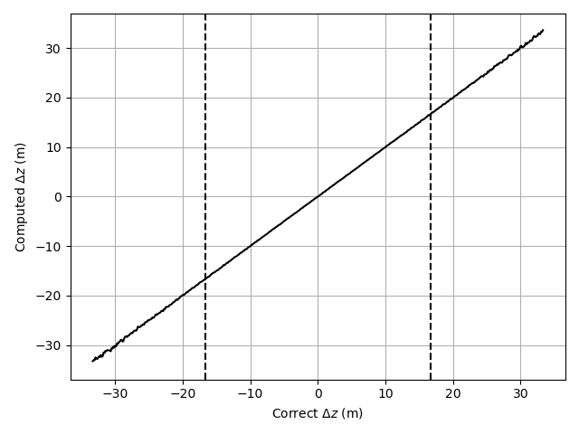
Consider the third-order polynomial aperture pictured in Fig. 1. Its length is 55.5m, and its height is 0.5m. Assume a center frequency of 9 GHz, and a range of 1km. A linear aperture of this length would have a horizontal resolution of 0.3m. Choose a hann window for $w_{\text{base}}(\tau)$. Using a single-frequency point-scatterer simulation, setting $\Delta x=\Delta y=0$, the computed vertical position matches the correct position with $\Delta z$ out to and somewhat beyond the dashed lines at $\pm 16.7m$, which are the edges of vertical resolution of a hypothetical rectangular aperture circumscribing the curve. Noise was added to each time sample, at an amplitude of 10% of that of the signal. Varying $\Delta x$ over the horizontal resolution of a linear aperture of this length ($\pm 0.15\text{m}$), and varying $\Delta y$ over the same amount (as might be expected for a SAR system), the error in computed $\Delta z$ is shown in Fig. 3. So the approximations we have introduced are capable of measuring $\Delta z$ to a high degree of accuracy in this setting, varying $\Delta x,\Delta y$ over the space of a SAR pixel, for a single scatterer, with a small amount of noise.

For a symmetric second-order polynomial aperture, either a height offset or a small range offset causes similar wavefronts to reach the aperture. For the full computation of (17), the ambiguity causes an ill-conditioned matrix. But if we make the assumption that $\Delta y$ is zero, we can modify (17) to remove both $\Delta y$ and (11), leaving

$$\begin{bmatrix}M_{00}&M_{02}\\ M_{10}&M_{12}\end{bmatrix}\begin{bmatrix}\Delta x\\ \Delta z\end{bmatrix}=\begin{bmatrix}b_{0}\\ b_{1}\end{bmatrix}.$$

(18)

A symmetric second-order polynomial aperture is shown in Fig. 4. The aperture height and length are the same as that of Fig. 1. Using (18), measured $\Delta z$ varies with small range offsets, as shown in Fig. (5). So the impact of dropping $\Delta y$ is that the vertical position estimate varies with small range offsets. The full CLAM computation using the aperture of Fig. (1) is immune to this ambiguity, as shown in (6). In certain applications and for certain apertures, the advantage of using a parabolic aperture may outweigh the impact of this ambiguity. In the case pictured, the vertical error is comparable to the size of the azimuthal resolution, which is typically comparable to the azimuthal resolution. But for some applications, this may be acceptible. Larger vertical apertures yield smaller ambiguities, for the same horizontal aperture. See Fig. (7) for results varying $\Delta x,\Delta y$ as in Fig. (3) The size of the errors are comparable for these parameters.

The computation for $\Delta x,\Delta y,\Delta z$ in (17) is nonlinear in the scalar field $E$, because $E$ is present in all terms of $\mathbf{M}$ and $\mathbf{b}$ in (17). For this reason, if multiple scatterers contribute to $E$, the computed values of $\Delta x,\Delta y,\Delta z$ are not a linear combination of the values that would be computed in the single-scatterer case. Nor are they guaranteed to be between or even near the correct values. This phenomenon is known as “glint” in the context of monopulse [12].

Consider a scatterer at $\Delta x=0,\Delta y=0,\Delta z=0$. If a “confuser” scatter is placed at the same $\Delta z=0$, but at some other $\Delta x,\Delta y$, then the measured $\Delta z$ is not necessarily near $0$. For the aperture of Fig. (1), the size of the error is shown in Fig. 8. $\Delta y$ is varied over half of a wavelength, because the phenomenon appears to be caused by the phase difference of the confuser. The horizontal resolution width is marked by dashed lines. The error is small for most phases, for most confuser scatterers within the resolution width. So a confuser scatterer in the same pixel is likely to result in the correct measurement. For confuser scatterers several resolution widths away, the directional effects of the backprojection function $h(\tau)$ rejects the energy from the confuser, and the measurement is approximately correct. However, for confuser scatterers only a few resolution widths away, the error can be quite large. This is because the beampatterns of many of the terms in (17) are wider than a resolution cell. Information from adjacent resolution cells are needed to make the measurement correctly. As a result of this, these computations will only be valid for scatterers that are particularly bright relative to their immediate surroundings in azimuth. SAR images often have pixels that are notably brighter than their neighbors, and this assumption is the basis of determining whether an image is in focus.

In a sensing context, it may be difficult to guarantee that only a single scatterer is represented in a location. We need a method to detect when a measurement is corrupted by “glint” from other scatterers. The determinant from the left side of (17) is shown in Fig. 9. Where this determinant is large, the glint error in Fig. 8 is small. This suggests that small determinants may be used to detect measurements corrupted by interference from other scatterers.

References

- [1] C. V. J. Jakowatz, D. E. Wahl, P. H. Eichel, D. C. Ghiglia, and P. A. Thompson, Spotlight-mode synthetic aperture radar: a signal processing approach. Springer Science & Business Media, 1996.
- [2] A. W. Doerry and D. L. Bickel, “Synthetic aperture radar height of focus.,” tech. rep., Sandia National Lab. (SNL-NM), Albuquerque, NM (United States), 2021.
- [3] A. W. Doerry and D. L. Bickel, “Impact of radar flightpath on synthetic aperture radar image height of focus,” in Radar Sensor Technology XXVI (K. I. Ranney and A. M. Raynal, eds.), vol. 12108, p. 121080V, International Society for Optics and Photonics, SPIE, 2022.
- [4] W. N. Barnes and T. H. Gauss, “Improved height above target (hat) measurement algorithm,” Nov. 3 1998. US Patent 6,831,563.
- [5] K. Knaell, “Three-dimensional SAR from curvilinear apertures,” in Algorithms for Synthetic Aperture Radar Imagery (D. A. Giglio, ed.), vol. 2230, pp. 120 – 134, International Society for Optics and Photonics, SPIE, 1994.
- [6] K. Knaell and G. Cardillo, “Radar tomography for the generation of three-dimensional images,” IEE Proceedings-Radar, Sonar and Navigation, vol. 142, no. 2, pp. 54–60, 1995.
- [7] K. Knaell, “Three-dimensional SAR from practical apertures,” in Radar/Ladar Processing and Applications, vol. 2562, pp. 31–41, International Society for Optics and Photonics, 1995.
- [8] C. D. Austin and R. L. Moses, “Wide-angle sparse 3D synthetic aerture radar imaging for nonlinear flight paths,” in 2008 IEEE National Aerospace and Electronics Conference, pp. 330–336, 2008.
- [9] J. A. Jackson and R. L. Moses, “Synthetic aperture radar 3D feature extraction for arbitrary flight paths,” IEEE Transactions on Aerospace and Electronic Systems, vol. 48, no. 3, pp. 2065–2084, 2012.
- [10] D. André, “An analysis of 3D SAR from single pass nonlinear radar platform trajectories,” in Algorithms for Synthetic Aperture Radar Imagery XVII, vol. 7699, pp. 71–82, SPIE, 2010.
- [11] T. Henderson, “Matched beam theory for unambiguous broadband direction finding,” The Journal of the Acoustical Society of America, vol. 78, no. 2, pp. 563–574, 1985.
- [12] T. L. Henderson and T. J. Brudner, “A space–time filtered gradient method for detecting directions of echoes and transient sounds,” The Journal of the Acoustical Society of America, vol. 118, no. 2, pp. 679–695, 2005.