Knowledge Distillation based Degradation Estimation for Blind Super-Resolution
Abstract
Blind image super-resolution (Blind-SR) aims to recover a high-resolution (HR) image from its corresponding low-resolution (LR) input image with unknown degradations. Most of the existing works design an explicit degradation estimator for each degradation to guide SR. However, it is infeasible to provide concrete labels of multiple degradation combinations (e.g., blur, noise, jpeg compression) to supervise the degradation estimator training. In addition, these special designs for certain degradation, such as blur, impedes the models from being generalized to handle different degradations. To this end, it is necessary to design an implicit degradation estimator that can extract discriminative degradation representation for all degradations without relying on the supervision of degradation ground-truth. In this paper, we propose a Knowledge Distillation based Blind-SR network (KDSR). It consists of a knowledge distillation based implicit degradation estimator network (KD-IDE) and an efficient SR network. To learn the KDSR model, we first train a teacher network: KD-IDET. It takes paired HR and LR patches as inputs and is optimized with the SR network jointly. Then, we further train a student network KD-IDES, which only takes LR images as input and learns to extract the same implicit degradation representation (IDR) as KD-IDET. In addition, to fully use extracted IDR, we design a simple, strong, and efficient IDR based dynamic convolution residual block (IDR-DCRB) to build an SR network. We conduct extensive experiments under classic and real-world degradation settings. The results show that KDSR achieves SOTA performance and can generalize to various degradation processes. The code is available at https://github.com/Zj-BinXia/KDSR.
1 Introduction
Single image super-resolution (SISR) aims to recover details of a high-resolution (HR) image from its low-resolution (LR) counterpart, which has a variety of downstream applications (Dong et al. 2014; Zhang et al. 2019; Xia et al. 2022d; Fritsche et al. 2019; Xia et al. 2022c; Xia et al. 2022b). These state-of-the-art methods (Kim et al. 2016; Lim et al. 2017; Lai et al. 2017; Xia et al. 2022a; Wang et al. 2018b) usually assume that there is an ideal bicubic downsampling kernel to generate LR images. However, this simple degradation is different from more complex degradations existing in real-world LR images. This degradation mismatch will lead to severe performance drops.
To address the issue, blind super-resolution (Blind-SR) methods are developed. Some Blind-SR works (Wang et al. 2021a; Luo et al. 2022) use the classical image degradation process, given by Eq. 1. Recently, some works (Cai et al. 2019; Bulat et al. 2018) attempted to develop a new and complex degradation process to better cover real-world degradation space, which forms a variant of Blind-SR called real-world super-resolution (Real-SR). The representative works include BSRGAN (Zhang et al. 2021) and Real-ESRGAN (Wang et al. 2021b), which introduce comprehensive degradation operations such as blur, noise, down-sampling, and JPEG compression, and control the severity of each operation by randomly sampling the respective hyper-parameters. To better simulate the complex degradations in real-world, they also apply random shuffle of degradation orders (Zhang et al. 2021) and second-order degradation (Wang et al. 2021b) respectively.
Since Blind-SR faces almost infinite degradations, introducing prior degradation information to SR networks can help to constrain the solution space and boost SR performance. As shown in Fig. 1, the way to obtain degradation information can be divided into three categories: (1) Several Non-Blind SR methods (Zhang et al. 2018a; Shocher et al. 2018; Zhang et al. 2020; Soh et al. 2020; Xu et al. 2020) directly take the known degradation information as prior (Fig. 1 (a)). (2) Most of Blind-SR methods (Gu et al. 2019; Luo et al. 2020; Wang et al. 2021a; Liang et al. 2022; Luo et al. 2022) adopt explicit degradation estimators, which are trained with ground-truth degradation (Fig. 1 (b)). However, these explicit degradation estimators are elaborately designed for specific degradation processes. The specialization makes them hard to transfer to handle other degradation processes. In addition, it is challenging to annotate precise ground-truth labels to represent the multiple degradation combination (Zhang et al. 2021; Wang et al. 2021b) for supervised degradation learning. Therefore, developing implicit degradation representation (IDR) based methods is important. (3) Recently, as shown in Fig. 1 (c), DASR (Wang et al. 2021a) and MM-RealSR (Mou et al. 2022) use metric learning to estimate IDR and quantize degradation severity respectively. However, metric learning methods roughly distinguish degradations by pushing away or pulling close features, which is unstable and cannot fully capture discriminative degradation characteristics for Blind-SR.

In this paper, we aim to design an efficient implicit degradation representation (IDR) learning SR framework that can easily adapt to any degradation process. To this end, we develop a novel knowledge distillation based Blind-SR Network (KDSR). Specifically, as shown in Fig. 1 (d), KDSR uses a knowledge distillation based implicit degradation estimator (KD-IDE) to predict accurate IDR. Furthermore, we propose a strong yet efficient SR network based on our newly developed IDR based Dynamic Convolution Residual Blocks (IDR-DCRB) to reconstruct the HR image with the guidance of IDR. For the training process, we first input HR and LR images to the teacher KD-IDET, which is optimized with the SR network together. Given the paired HR and LR images, teacher KD-IDET can easily extract the latent degradation information in LR images. Then, we use a student KD-IDES to learn to extract the same IDR as that of KD-IDET from LR images directly. Extensive experiments can demonstrate the effectiveness of the proposed KDSR. Our main contributions are threefold:
- •
We propose KDSR, a strong, simple, and efficient baseline for Blind-SR, can generalize to any degradation process, which addresses the weakness of explicit degradation estimation.
- •
We propose a novel KD based implicit degradation representation (IDR) estimator. To the best of our knowledge, the design of IDR estimation has received little attention so far. Besides, we propose an efficient IDR-based SR network to fully utilize IDR to guide SR.
- •
Extensive experiments show that the proposed KDSR can achieve excellent Blind-SR performance in different degradation settings from simple to complex.
2 Related Work
2.1 Blind Super-Resolution
In the past few years, numerous Non-Blind SISR methods (Dong et al. 2014; Lim et al. 2017; Zhang et al. 2018a; Ledig et al. 2017; Johnson et al. 2016; Ma et al. 2020; Xia et al. 2023) have achieved promising performance and have been widely studied. However, the performance of these methods will dramatically decline as there is a degradation gap between training and test data. As a remedy, SRMD (Zhang et al. 2018a), USRNet (Zhang et al. 2020) and some other methods (Zhang et al. 2019; Xu et al. 2020; Shocher et al. 2018; Soh et al. 2020) utilize the blur kernel and noise level as additional input. Although these methods can deal with multiple degradations with a single model, they require accurate degradation estimation, which is also a challenging task.
To handle unknown degradation, a few Blind-SR methods have been proposed. Some methods, such as IKC (Gu et al. 2019) and DAN (Luo et al. 2020), use the classical Blind-SR degradation process and combine a blur kernel estimator with SR networks, which can be adaptive to images degraded from various blur kernels (Kim et al. 2021; Cornillere et al. 2019). Besides, KMSR (Zhou & Susstrunk 2019) constructs a kernel pool by utilizing a generative adversarial network (Goodfellow et al. 2014). Recently, some works like BSRGAN (Zhang et al. 2021) and Real-ESRGAN (Wang et al. 2021b) design more complex and comprehensive degradation processes to better cover the real-world degradation space, which becomes a variant of Blind-SR called Real-SR.
For each degradation type and process, previous Blind-SR methods (Gu et al. 2019; Liang et al. 2022) tend to specially design an explicit degradation estimator. That is quite complex and hard to provide ground-truth labels for multiple degradation combinations. Recently, DASR (Wang et al. 2021a) and MM-RealSR (Mou et al. 2022) use metric learning to roughly distinguish various degradations, which is not accurate enough to provide degradation representation to guide SR. In this paper, we propose to estimate IDR accurately and fully use it for SR in an efficient way.
2.2 Knowledge Distillation
The purpose of knowledge distillation (KD) (Hinton et al. 2015) is to transfer the representation ability of a teacher network to a student network. KD has been widely used to compress models, typically for classification tasks. Specifically, they (Ahn et al. 2019) compress the classification models by enforcing the output distribution between the teacher and student networks to be close. Recently, some works extend KD to feature distillation, such as intermediate feature learning (Romero et al. 2014) and pairwise relations in intermediate feature learning (Liu et al. 2019). For the SISR task, SRKD (Gao et al. 2018) and FAKD (He et al. 2020) apply the KD between intermediate feature maps to compress models. To obtain more efficient SR networks, PISR (Lee et al. 2020) further introduces variational information distillation (Ahn et al. 2019) to maximize the mutual information between intermediate feature maps of teacher and student SR networks. Different from previous works adopting KD for model compression, we develop KDSR to obtain accurate IDR.
3 Methodology
In this section, we present our knowledge distillation based Blind-SR network, i.e., KDSR. As shown in Fig. 2, KDSR mainly consists of a knowledge distillation based implicit degradation estimator network (KD-IDE) and a SR network. In the following sections, we first introduce the blind-SR problems in Sec. 3.1. Then, we provide the details of the proposed KD-IDE and SR networks of KDSR in Sec. 3.2 and Sec. 3.3, respectively. In Sec. 3.4, we introduce the two-stage training details.
3.1 Overview
Blind SR methods can be summarized two categories: classic blind-SR and real-world blind-SR.
For classic blind-SR, some Blind-SR works (Wang et al. 2021a; Luo et al. 2022) use the classical image degradation process, given by
| (1) |
where denotes convolution operation. and are HR and corresponding LR images respectively. is blur kernel and is additional white Gaussian noise. refers to downsampling operation with scale factor . The severity of blur and noise are unknown, which randomly sampling the respective hyper-parameters to adjust severity and form almost infinite degradation space.
Given an input LR image and applied blur kernel , the classic blind-SR methods (Gu et al. 2019; Luo et al. 2020; Luo et al. 2022) pretrain an explicit degradation estimator to estimate the blur kernel applied on with the supervision of groundtruth . Then, their SR network can use the estimated blur kernel to perform SR on LR image . The SR network is trained with loss function .
| (2) |
where and are real and SR images separately.
Real-world blind-SR is a variant of classic blind-SR, in which more complicated degradation is adopted. The real-world blind-SR approaches (Wang et al. 2021b; Zhang et al. 2021) introduce comprehensive degradation operations such as blur, noise, down-sampling, and JPEG compression, and control the severity of each operation by randomly sampling the respective hyper-parameters. Moreover, they apply random shuffle of degradation orders and second-order degradation to increase degradation complexity. Since degradation is complex and cannot provide specific degradation labels, they directly use SR networks without degradation estimators. Their SR networks emphasize visual quality trained with .
| (3) |
where and are perceptual (Johnson et al. 2016) and adversarial loss (Wang et al. 2021b).
As shown in Fig. 2, we propose a KDSR, consisting of KD-IDE and an efficient SR network. Different previous explicit degradation estimation based blind-SR methods Gu et al. 2019; Luo et al. 2020; Luo et al. 2022; Liang et al. 2022, our KD-IDE does not requires degradation labels for training, which can generalize to any degradation process. Moreover, our the design of our SR network is neat and efficient, which is practical and can fully use degradation information for SR. There are two stage training processes for KDSR, including Teacher KDSRT and Student KDSRS training. We first train the KDSRT: we input the paired HR and LR images to the KD-IDET and obtain the implicit degradation representation (IDR) and , where is used to guide the SR. After that, we move on to KDSRS training. We initialize the KDSRS with the KDSRT’s parameters and make the KDSRS learn to directly extract same as from LR images.
3.2 Knowledge Distillation based Implicit Degradation Estimator
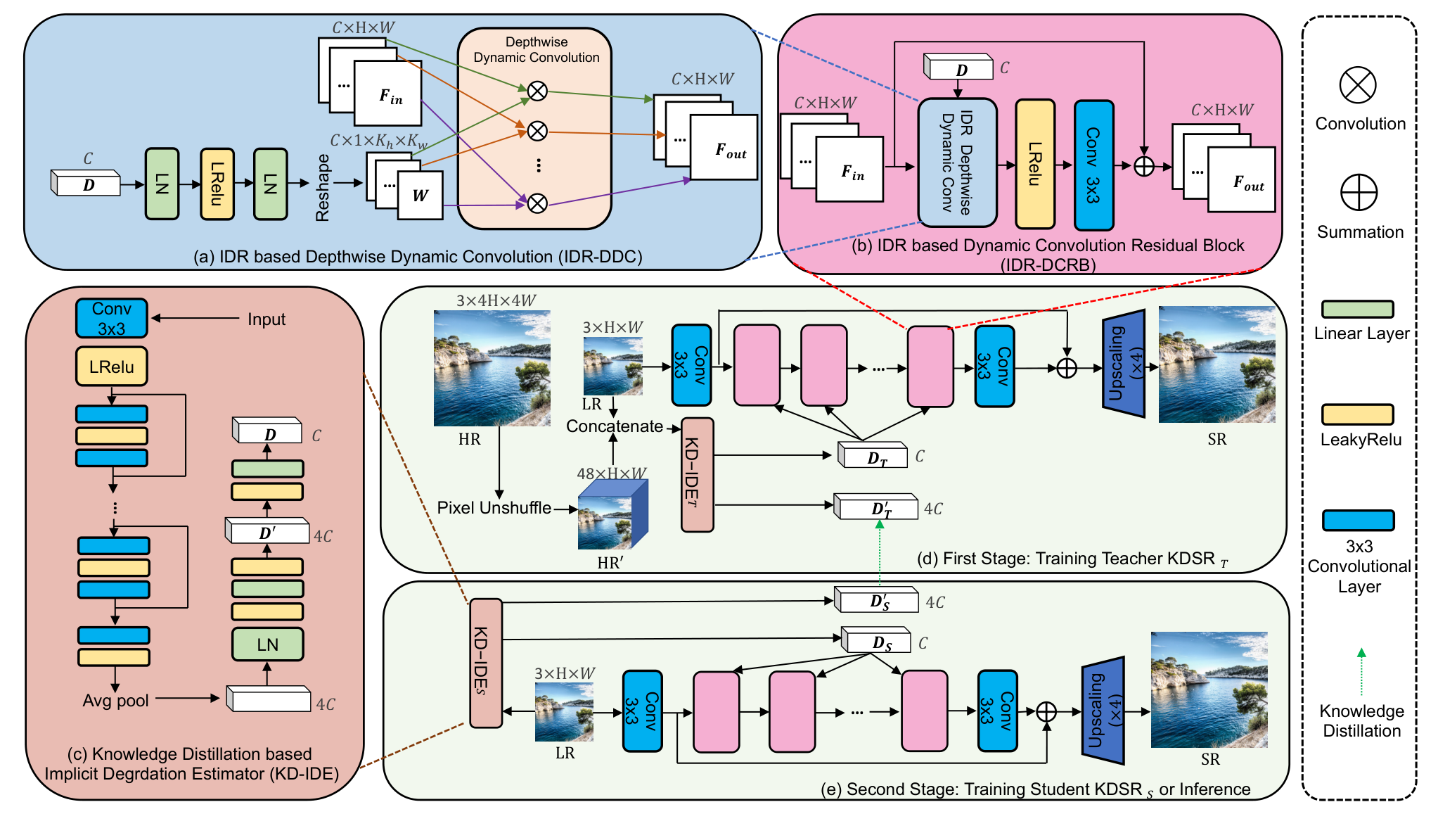
Most Blind-SR methods elaborately design an explicit degradation estimator for each degradation type and process. There are several limitations for explicit degradation estimators: (1) These special designs for specific degradation processes make the explicit estimator hard to be transferred to other degradation settings. (2) It is complex to provide various degradation labels for explicit degradation estimator training, especially the random combination of multiple degradations (Wang et al. 2021b). Therefore, we develop a KD based implicit degradation estimator (KD-IDE), which can distinguish various degradations accurately without the supervision of degradation ground-truth.
As shown in Fig. 2 (c), we can divide KD-IDE into several parts: (1) We take the LR images and the concatenation of LR and HR images as input for KD-IDES and KD-IDET, respectively. Specially, for the KD-IDET (Fig. 2 (d)), it can easily extract the degradation which makes HR degrade to LR images by providing paired HR and LR images and jointly being optimized with the SR network. Since there is a spatial size difference between HR and LR images, we perform the Pixel-Unshuffle operation on HR images to be and then concatenate it with LR images to obtain an input . (2) The input passes through the first convolution to become feature maps. It is noticeable that the input channels in the first convolution are 3 and 51 for KD-IDES and KD-IDET, respectively. (3) After that, we use numerous residual blocks to further extract features and obtain a rough degradation vector by Average Pooling operation. (4) We use the two linear layers to refine the degradation vector and obtain IDR , which is used for KD. (5) Although has channels to accurately present degradation and can give more degradation information for the student network to learn, it will consume a large number of computational resources used in IDR-DDC. Hence, we need to further compress it with a linear layer and obtain another IDR to guide SR. More details of KD training are given in Sec. 3.4.
3.3 Image Super-Resolution Network
As for the design of SR network, we should consider three points: (1) After we obtain the IDR, it is important to design a SR network that can fully use the estimated degradation prior for SR. (2) An ideal Blind-SR network is likely to be used in practice, the structure of which should be simple. Thus, we also try to make the network formed by one type of simple and strong enough module. (3) The huge computation consumption usually limits the application of models, especially on edge devices. Thus, it is necessary to design an efficient model.
As shown in Fig. 2 (a), (b), and (d), our SR network can be divided into three hierarchies. (1) We first propose a convolution unit called IDR based Depthwise Dynamic Convolution (IDR-DDC). Motivated by UDVD (Xu et al. 2020), we adopt the dynamic convolution to use IDR to guide SR. Specifically, to fully use the estimated IDR, as displayed in Fig. 2 (a), we generate specific convolution weights according to the IDR . However, if we generate ordinary convolution weights, the computational cost will be quite large and affect the efficiency of the network. Thus, we further introduce depthwise convolution (Howard et al. 2017), which merely consumes about computation and parameters of ordinary convolution. The IDR-DDC can be mathematically expressed as:
| (4) |
| (5) |
where and are two linear layers and convolution operation separately; indicates IDR, is the output of , is weights of dynamic convolution ; and are input and output feature maps respectively. (2) As shown in Fig. 2 (b), motivated by EDSR (Lim et al. 2017), we develop IDR based Dynamic Convolution Residual Blocks (IDR-DCRB) to realize deep model. For the first convolution of IDR-DCRB, we use the IDR-DDC to utilize degradation information. However, IDR-DDC lacks interaction between different channels. Thus, we adopt ordinary convolution as the second convolution. (3) For simplicity, as shown in Fig. 2 (d) or (e), we mainly stack the IDR-DCRB to form the SR network.
3.4 Training Process
KDSR has a two-stage training process. (1) As shown in the Fig. 2 (d), we first train the teacher KDSRT. we input the paired LR and HR images to the KD-IDET obtain the IDR and . Then, is used to generate specific degradation weights for dynamic convolution. After that, the specific degradation SR network will restore the LR images. By jointly optimizing the teacher SR network and KD-IDET with the Loss (Eq. 2), the KD-IDE can effectively extract accurate IDR to guide SR network. (2) After finishing KDSRT training, we move on to train KDSRS. As shown in the Fig. 2 (e), different from KD-IDET, we only input the LR images to the KD-IDES, obtaining IDR and . The other steps are the same as KDSRT training except for the adopted loss functions. Specifically, we introduce a knowledge distillation (KD) function (Eq. 6) to enforce the KD-IDES directly extracting the same accurate IDR as KD-IDET from LR images. In addition, for the classic degradation model (Eq. 1), following previous Blind-SR works (Gu et al. 2019; Wang et al. 2021a), we adopt (Eq. 2) and can set the total loss function as (Eq. 7). For more complex degradation processes (Real-SR), following (Eq. 3) of Real-ESRGAN (Wang et al. 2021b), we propose (Eq. 8). More details are given in appendix.
| (6) |
| (7) |
| (8) |
where and are normalized with softmax operation of and separately. and are perceptual and adversarial loss. , and denote the balancing parameters.
4 Experiments
4.1 Settings
We train and test our method on classic and real-world degradation settings. For the , following previous works (Gu et al. 2019; Luo et al. 2022), we combine 800 images in DIV2K (Agustsson & Timofte 2017) and 2,650 images in Flickr2K (Timofte et al. 2017) as the DF2K training set. The batch sizes are set to 64, and the LR patch sizes are 6464. We use Adam optimizer with , . We train both teacher and student networks with 600 epochs and set their initial learning rate to and decrease to half after every 150 epochs. The loss coefficient and are set to 1 and 0.15 separately. The SR results are evaluated with PSNR and SSIM on the Y channel in the YCbCr space. (1) In Sec. 4.2, we train and test on isotropic Gaussian kernels following the setting in Gu et al. 2019. Specifically, the kernel sizes are fixed to 2121. In training, the kernel width ranges are set to [0.2, 4.0] for scale factors 4. We uniformly sample the kernel width in the above ranges. For testing, we adopt the Gaussian8 (Gu et al. 2019) kernel setting to generate evaluation datasets. Gaussian8 uniformly chooses 8 kernels from range [1.80, 3.20] for scale 4. The LR images are obtained by blurring and downsampling the HR images with selected kernels. (2) In Sec. 4.3, we also validate our methods on anisotropic Gaussian kernels and noises following the setting in (Wang et al. 2021a). Specifically, We set the kernel size to 2121 for scale factor 4. In training, we use the additive Gaussian noise with covariance and adopt anisotropic Gaussian kernels characterized by Gaussian probability density function with zero mean and varying covariance matrix . The covariance matrix is determined by two random eigenvalues and a random rotation angle .
For the -, in Sec. 4.4, similar to Real-ESRGAN (Wang et al. 2021b), we adopt DF2K and OutdoorSceneTraining (Wang et al. 2018a) datasets for training. We set the learning rate of the KDSRT to and pre-train it with only Eq. 2 by 1000K iterations. Then, we optimize KDSRS with Eq. 7 by 1000K iterations and continue to train it with Eq. 8 by 400K iterations. The learning rate is fixed as . For optimization, we use Adam with , . In both two stages of training, we set the batch size to 48, with the input patch size being 64.
| Methods | Param (M) | FLOPs (G) | Time (ms) | Set5 | Set14 | BSD100 | Urban100 | Manga109 | |||||
| PSNR | SSIM | PSNR | SSIM | PSNR | SSIM | PSNR | SSIM | PSNR | SSIM | ||||
| Bicubic | - | - | - | 24.57 | 0.7108 | 22.79 | 0.6032 | 23.29 | 0.5786 | 20.35 | 0.5532 | 21.50 | 0.6933 |
| RCAN | 15.59 | 1082.41 | 556.21 | 26.60 | 0.7598 | 24.85 | 0.6513 | 25.01 | 0.6170 | 22.19 | 0.6078 | 23.52 | 0.7428 |
| Bicubic+ZSSR | 0.23 | - | 30946.60 | 26.45 | 0.7279 | 24.78 | 0.6268 | 24.97 | 0.5989 | 21.11 | 0.5805 | 23.53 | 0.724 |
| IKC | 5.32 | 2528.03 | 1053.79 | 31.67 | 0.8829 | 28.31 | 0.7643 | 27.37 | 0.7192 | 25.33 | 0.7504 | 28.91 | 0.8782 |
| DANv1 | 4.33 | 1098.33 | 201.04 | 31.89 | 0.8864 | 28.42 | 0.7687 | 27.51 | 0.7248 | 25.86 | 0.7721 | 30.50 | 0.9037 |
| DANv2 | 4.71 | 1088.14 | 201.51 | 32.00 | 0.8885 | 28.50 | 0.7715 | 27.56 | 0.7277 | 25.94 | 0.7748 | 30.45 | 0.9037 |
| AdaTarget | 16.70 | 1032.59 | 109.77 | 31.58 | 0.8814 | 28.14 | 0.7626 | 27.43 | 0.7216 | 25.72 | 0.7683 | 29.97 | 0.8955 |
| DCLS | 13.63 | - | 175.84 | 32.12 | 0.8890 | 28.54 | 0.7728 | 27.60 | 0.7285 | 26.15 | 0.7809 | 30.86 | 0.9086 |
| DASR | 5.84 | 185.66 | 44.14 | 31.46 | 0.8789 | 28.11 | 0.7603 | 27.44 | 0.7214 | 25.36 | 0.7506 | 29.39 | 0.8861 |
| KDSRS-M (Ours) | 5.80 | 191.42 | 38.74 | 32.02 | 0.8892 | 28.46 | 0.7761 | 27.52 | 0.7281 | 25.96 | 0.7760 | 30.58 | 0.9026 |
| KDSRS-L (Ours) | 14.19 | 623.61 | 149.14 | 32.11 | 0.8933 | 28.68 | 0.7867 | 27.64 | 0.7300 | 26.15 | 0.7830 | 30.99 | 0.9069 |


 HR
RCAN
DCLS
KDSRS-M
HR
RCAN
DCLS
KDSRS-M


 Bicubic
DANv2
DASR
KDSRS-L
Bicubic
DANv2
DASR
KDSRS-L


 HR
RCAN
DCLS
KDSRS-M
HR
RCAN
DCLS
KDSRS-M


 Bicubic
DANv2
DASR
KDSRS-L
Bicubic
DANv2
DASR
KDSRS-L
|


 HR
RCAN
DCLS
KDSRS-M
HR
RCAN
DCLS
KDSRS-M


 Bicubic
DANv2
DASR
KDSRS-L
Bicubic
DANv2
DASR
KDSRS-L


 HR
RCAN
DCLS
KDSRS-M
HR
RCAN
DCLS
KDSRS-M


 Bicubic
DANv2
DASR
KDSRS-L
Bicubic
DANv2
DASR
KDSRS-L
|
4.2 Evaluation with Isotropic Gaussian Kernels
We first evaluate our KDSR on degradation with isotropic Gaussian kernels. We compare the KDSR with several SR methods, including RCAN (Zhang et al. 2018c), ZSSR (Shocher et al. 2018), IKC (Gu et al. 2019), DAN (Luo et al. 2020), AdaTarget (Jo et al. 2021), and DASR (Wang et al. 2021a). Note that RCAN is a state-of-the-art SR method for bicubic degradation. For a fair comparison on different model sizes, we develop KDSRS-M and KDSRS-L by adjusting the depth and channels of the network. We apply Gaussian8 (Gu et al. 2019) kernel setting on five datasets, including Set5 (Bevilacqua et al. 2012), Set14 (Zeyde et al. 2010), B100 (Martin et al. 2001), Urban100 (Huang et al. 2015), and Manga109 (Matsui et al. 2017), to generate evaluation datasets.
The quantitative results are shown in Tab. 1. We can see that our KDSRS-M surpasses DASR by 0.6dB, 0.39dB, 0.67dB and 1.24dB on Set5, Set14, Urban100 and Manga109 datasets separately. In addition, compared with the Blind-SR method DANv2, our KDSRS-M achieves better performance consuming only FLOPs of DANv2. It is because that DANv2 uses an iterative strategy to estimate accurate explicit blur kernels, which requires many computations. Besides, compared with the SOTA Blind-SR method DCLS, our KDSRS-L achieves better performance on almost all datasets consuming less time. It is notable that DCLS specially designed an explicit degradation estimator for blur kernel, while the KD-IDE in our KDSR is simple and can adapt to any degradation process. The qualitative results are shown in Fig. 3. We can see that our KDSRS-L has more clear textures compared with other methods. Our KDSRS-M also achieves better visual results than DANv2.
| Method | Params | Time | Noise | Blur Kernel | ||||||||
|---|---|---|---|---|---|---|---|---|---|---|---|---|
![[Uncaptioned image]](2211.16928v2/table2_kernel/1.png) |
![[Uncaptioned image]](2211.16928v2/table2_kernel/2.png) |
![[Uncaptioned image]](2211.16928v2/table2_kernel/3.png) |
![[Uncaptioned image]](2211.16928v2/table2_kernel/4.png) |
![[Uncaptioned image]](2211.16928v2/table2_kernel/5.png) |
![[Uncaptioned image]](2211.16928v2/table2_kernel/6.png) |
![[Uncaptioned image]](2211.16928v2/table2_kernel/7.png) |
![[Uncaptioned image]](2211.16928v2/table2_kernel/8.png) |
![[Uncaptioned image]](2211.16928v2/table2_kernel/9.png) | ||||
| DnCNN + RCAN | 650K+15.59M | 556.21ms | 0 | 24.28 | 24.47 | 24.6 | 24.64 | 24.58 | 24.47 | 24.31 | 23.97 | 23.01 |
| 10 | 23.88 | 24.03 | 24.16 | 24.21 | 24.13 | 24.03 | 23.88 | 23.62 | 22.76 | |||
| 20 | 23.45 | 23.58 | 23.70 | 23.73 | 23.69 | 23.57 | 23.42 | 23.23 | 22.46 | |||
| DnCNN +IKC | 650K+5.32M | 1053.79ms | 0 | 24.76 | 25.55 | 26.54 | 27.33 | 26.55 | 25.55 | 24.64 | 25.99 | 25.49 |
| 10 | 24.20 | 24.54 | 24.86 | 24.96 | 24.78 | 24.52 | 24.23 | 24.19 | 23.14 | |||
| 20 | 23.62 | 23.87 | 24.07 | 24.15 | 24.06 | 23.86 | 23.65 | 23.59 | 22.71 | |||
| DnCNN +DCLS | 650K+19.05M | 192.83ms | 0 | 25.80 | 26.20 | 26.45 | 26.46 | 26.30 | 26.20 | 26.39 | 25.57 | 23.96 |
| 10 | 24.05 | 24.28 | 24.44 | 24.50 | 24.40 | 24.27 | 24.09 | 23.85 | 22.90 | |||
| 20 | 23.58 | 23.75 | 23.88 | 23.93 | 23.88 | 23.72 | 23.56 | 23.40 | 22.58 | |||
| DASR | 5.84M | 44.14ms | 0 | 27.20 | 27.62 | 27.74 | 27.85 | 27.82 | 27.62 | 27.38 | 27.44 | 26.27 |
| 10 | 25.26 | 25.57 | 25.64 | 25.69 | 25.62 | 25.54 | 25.42 | 25.20 | 24.37 | |||
| 20 | 23.68 | 23.87 | 24.20 | 24.32 | 24.09 | 23.91 | 23.76 | 23.81 | 22.87 | |||
| KDSRS (Ours) | 5.80M | 38.74ms | 0 | 27.67 | 27.99 | 28.14 | 28.20 | 28.12 | 27.99 | 27.80 | 27.87 | 26.52 |
| 10 | 25.74 | 25.91 | 25.97 | 26.00 | 25.96 | 25.88 | 25.75 | 25.50 | 24.67 | |||
| 20 | 24.72 | 24.89 | 24.92 | 24.89 | 24.92 | 24.82 | 24.70 | 24.59 | 23.84 | |||


 HR
DCLS
DASR
HR
DCLS
DASR


 Bicubic
RCAN
KDSRS
Bicubic
RCAN
KDSRS


 HR
DCLS
DASR
HR
DCLS
DASR


 Bicubic
RCAN
KDSRS
Bicubic
RCAN
KDSRS
|
4.3 Evaluation with Anisotropic Gaussian Kernels and Noises
We evaluate our KDSR on degradation with anisotropic Gaussian kernels and noises by adopting 9 typical blur kernels and different noise levels. We compare our KDSR with SOTA blind-SR methods, including RCAN (Zhang et al. 2018c), IKC (Gu et al. 2019), DCLS (Luo et al. 2022) and DASR (Wang et al. 2021a). Since RCAN, IKC, and DCLS cannot deal with noise degradation, we use DnCNN (Zhang et al. 2017), a SOTA denoising method, to denoise images for them.
The quantitative results are shown in Tab. 2. Compared with the SOTA explicit degradation estimation based on Blind-SR methods DCLS, our KDSRS surpasses it by over 1 dB under almost all degradation settings consuming parameters and runtime. Furthermore, as , our KDSRS surpasses DASR by about 1dB with less parameters and runtime. This shows the superiority of knowledge distillation based IDR estimation and efficient SR network structure. In addition, we provide visual comparison in Fig. 4. We can see that KDSRS has sharper edges, more realistic details, and fewer artifacts compared with other methods. More visual results are given in appendix.
4.4 Evaluation on Real-World SR
We further validate the effectiveness of KDSR on Real-World datasets. As described in Sec. 4.1, we introduce GAN (Goodfellow et al. 2014) and perceptual Johnson et al. 2016 loss to train our network with the same high-order complex degradation process as Real-ESRGAN (Wang et al. 2021b), obtaining KDSRS-GAN. We compare our methods with the state-of-the-art GAN-based SR methods, including Real-ESRGAN, BSRGAN (Zhang et al. 2021), MM-RealSR (Mou et al. 2022), ESRGAN (Wang et al. 2018b). We evaluate all methods on the dataset provided in the challenge of Real-World Super-Resolution: AIM19 Track2 (Lugmayr et al. 2019) and NTIRE2020 Track1 (Lugmayr et al. 2020). Since AIM19 and NTIRE2020 datasets provide a paired validation set, we use the LPIPS (Zhang et al. 2018b), PSNR, and SSIM for the evaluation.
The quantitative results are shown in Tab. 3. Compared with the recent real-world SR method MM-RealSR, our KDSRS-GAN performs better, only consuming about 50 runtime. In addition, KDSRS-GAN outperforms SOTA real-world SR method Real-ESRGAN on LPIPS, PSNR, and SSIM, only consuming its 75 FLOPs. Furthermore, we provide qualitative results in Fig. 5. We can see that our KDSRS-GAN produces more visually promising results with clearer details and textures. More qualitative results are provided in appendix.
| Methods | Parms (M) | FLOPs(G) | Runtime (ms) | AIM2019 | NTIRE2020 | ||||
| LPIPS | PSNR | SSIM | LPIPS | PSNR | SSIM | ||||
| ESRGAN | 16.69 | 871.25 | 236.04 | 0.5558 | 23.17 | 0.6192 | 0.5938 | 21.14 | 0.3119 |
| BSRGAN | 16.69 | 871.25 | 236.04 | 0.4048 | 24.20 | 0.6904 | 0.3691 | 26.75 | 0.7386 |
| Real-ESRGAN | 16.69 | 871.25 | 236.04 | 0.3956 | 23.89 | 0.6892 | 0.3471 | 26.40 | 0.7431 |
| MM-RealSR | 26.13 | 930.54 | 290.64 | 0.3948 | 23.45 | 0.6889 | 0.3446 | 25.19 | 0.7404 |
| KDSRs-GAN (Ours) | 18.85 | 640.84 | 154.62 | 0.3758 | 24.22 | 0.7038 | 0.3198 | 27.12 | 0.7614 |


 HR
BSRGAN
MM-RealSR
HR
BSRGAN
MM-RealSR


 Bicubic
Real-ESRGAN
KDSRS-GAN
Bicubic
Real-ESRGAN
KDSRS-GAN


 HR
BSRGAN
MM-RealSR
HR
BSRGAN
MM-RealSR


 Bicubic
Real-ESRGAN
KDSRS-GAN
Bicubic
Real-ESRGAN
KDSRS-GAN
|
5 Ablation Study
Knowledge Distillation Based Blind-SR Network. In this part, we validate the effectiveness of the components in KDSR, such as KD and IDR-DDC (Tab. 4). KDSRS4 is actually the KDSRS-M adopted in Tab. 1, and KDSRT is KDSRT4’s corresponding teacher network. (1) We directly input the degradation blur kernels into the KDSRS4, obtaining KDSRS3. Compared with KDSRS3, KDSRS4 has a similar performance by estimating IDR. That demonstrates that our KDSRS4 can estimate quite accurate IDR to guide Blind-SR. (2) We cancel the KD in KDSRS4 to obtain KDSRS2, which means that KDSRS2 cannot learn the IDR extraction from KDSRT. Comparing KDSRS4 and KDSRS2, we can see that the KD scheme can bring 0.42dB improvement for KDSRS4, which demonstrates that KD can effectively help KDSRS4 to learn the IDR extraction ability from KDSRT. (3) Based on KDSRS2, we replace the IDR-DDC in IDR-DCRB with ordinary convolution to obtain KDSRS1. KDSRS2 is 0.17dB higher than KDSRS1, which demonstrates the effectiveness of IDR-CDC. (4) Besides, KDSRS4 is 0.2dB lower than its teacher KDSRT. That means KDSRS4 cannot completely learn the IDR extraction ability from KDSRT.
| Method | Oracle Degradation | KD | IDR-DDC | Param (M) | FLOPs (G) | Time (ms) | PSNR (dB) |
| KDSRT (Ours) | ✗ | ✗ | ✓ | 5.82 | 192.77 | 39.05 | 26.16 |
| KDSRS1 | ✗ | ✗ | ✗ | 5.58 | 293.46 | 47.80 | 25.37 |
| KDSRS2 | ✗ | ✗ | ✓ | 5.80 | 191.42 | 38.74 | 25.54 |
| KDSRS3 | ✓ | ✗ | ✓ | 6.13 | 166.26 | 41.06 | 26.08 |
| KDSRS4 (Ours) | ✗ | ✓ | ✓ | 5.80 | 191.42 | 38.74 | 25.96 |
The Loss Functions for Knowledge Distillation. We explore which KD function is best to guide the KDSRS learn to directly extract the same IDR as KDSRT from LR images. Although there are some works (Gao et al. 2018; He et al. 2020) have explored the KD function for SR, they take intermediate feature maps as learning objects to compress SR models. However, we take IDR as learning objects to learn the ability to extract IDR from LR images. Therefore, we cannot directly apply these experiences from previous works to our model. Here, we define three classic KD functions: (1) We use the Kullback Leibler divergence to measure distribution similarity (, Eq. 6). (2) We define for optimization (Eq. 9). (3) Motivated by KD loss in SR model compression (Gao et al. 2018), we define (Eq. 10).
| (9) |
| (10) |
where and are IDRs extracted by KDSRT-M and KDSRS-M respectively. We apply these three loss functions on KDSRS-M separately to learn the IDR from KDSRT-M. Then, we evaluate them on 4 Urban100 with Gaussian8 kernels. The results are shown in Tab. 5. We can see that the performance of is better than and . That means that the degradation information is mainly contained in the distribution of IDR rather than in its absolute values.
The Visualization of KD-IDE. To further validate the effectiveness of our KD-IDE, we use t-SNE (Van der Maaten & Hinton 2008) to visualize the distribution of extracted IDR. Specifically, we generate LR images from BSD100 (Martin et al. 2001) with different isotropic Gaussian kernels and feed them to KDSRT, KDSRS, KDSRS without KD, and DASR (Wang et al. 2021a) to generate IDR for Fig. 6 (a), (b), (c), and (d) respectively. We can see from Fig. 6 (a) and (b) that KDSRT can distinguish different degradations, and KDSRS also learn this ability from KDSRT well. In addition, comparing Fig. 6 (b) and (c), we can see that KDSRS obtaining IDR extraction knowledge from KDSRT can distinguish various degradations better than KDSRS without adopting KD. That further demonstrates the effectiveness of our KD-IDE. Furthermore, we compare KDSRS and DASR (Fig. 6 (b) and (d)), and the results show that KDSRS can distinguish various degradations more clear than DASR, which shows the superiority of KD based IDE to metric learning based IDE.
 | ||||
| (a) IDR extracted by KDSRT. | (b) IDR extracted by KDSRS. | (c) IDR extracted by KDSRS without KD. | (d) IDR extracted by DASR. |
6 Conclusion
Most Blind-SR methods tend to elaborately design an explicit degradation estimator for a specific type of degradation to guide SR. Nevertheless, it is difficult to provide the labels of multiple degradation combinations to train explicit degradation estimators, and these specific designs for certain degradation make them hard to transfer to other degradation processes. To address these issues, we develop a knowledge distillation based Blind-SR (KDSR) network, consisting of a KD-IDE and an efficient SR network that is stacked by IDR-DCRBs. We use KD to make KD-IDES directly extract the same accurate IDR as KD-IDET from LR images. IDR-DCRBs of SR network use IDR based depthwise dynamic convolution to fully and efficiently utilize the extracted IDR to guide SR. Extensive experiments on classic and complex real-world degradation processes demonstrate that the proposed KDSR can achieve a general state-of-the-art Blind SR performance.
Acknowledgments
This work was partly supported by the Alexander von Humboldt Foundation, the National Natural Science Foundation of China(No. 62171251), the Natural Science Foundation of Guangdong Province(No.2020A1515010711), the Special Foundations for the Development of Strategic Emerging Industries of Shenzhen(Nos.JCYJ20200109143010272 and CJGJZD20210408092804011) and Oversea Cooperation Foundation of Tsinghua.
References
- Agustsson & Timofte (2017) Eirikur Agustsson and Radu Timofte. Ntire 2017 challenge on single image super-resolution: Dataset and study. In CVPRW, 2017.
- Ahn et al. (2019) Sungsoo Ahn, Shell Xu Hu, Andreas Damianou, Neil D Lawrence, and Zhenwen Dai. Variational information distillation for knowledge transfer. In CVPR, 2019.
- Bevilacqua et al. (2012) Marco Bevilacqua, Aline Roumy, Christine Guillemot, and Marie line Alberi Morel. Low-complexity single-image super-resolution based on nonnegative neighbor embedding. In BMVC, 2012.
- Bulat et al. (2018) Adrian Bulat, Jing Yang, and Georgios Tzimiropoulos. To learn image super-resolution, use a gan to learn how to do image degradation first. In ECCV, 2018.
- Cai et al. (2019) Jianrui Cai, Hui Zeng, Hongwei Yong, Zisheng Cao, and Lei Zhang. Toward real-world single image super-resolution: A new benchmark and a new model. In ICCV, 2019.
- Cornillere et al. (2019) Victor Cornillere, Abdelaziz Djelouah, Wang Yifan, Olga Sorkine-Hornung, and Christopher Schroers. Blind image super-resolution with spatially variant degradations. TOG, 2019.
- Dong et al. (2014) Chao Dong, Chen Change Loy, Kaiming He, and Xiaoou Tang. Learning a deep convolutional network for image super-resolution. In ECCV, 2014.
- Fritsche et al. (2019) Manuel Fritsche, Shuhang Gu, and Radu Timofte. Frequency separation for real-world super-resolution. In ICCVW, 2019.
- Gao et al. (2018) Qinquan Gao, Yan Zhao, Gen Li, and Tong Tong. Image super-resolution using knowledge distillation. In ACCV, 2018.
- Goodfellow et al. (2014) Ian Goodfellow, Jean Pouget-Abadie, Mehdi Mirza, Bing Xu, David Warde-Farley, Sherjil Ozair, Aaron Courville, and Yoshua Bengio. Generative adversarial nets. NeurIPS, 2014.
- Gu et al. (2019) Jinjin Gu, Hannan Lu, Wangmeng Zuo, and Chao Dong. Blind super-resolution with iterative kernel correction. In CVPR, 2019.
- He et al. (2020) Zibin He, Tao Dai, Jian Lu, Yong Jiang, and Shu-Tao Xia. Fakd: Feature-affinity based knowledge distillation for efficient image super-resolution. In ICIP, 2020.
- Hinton et al. (2015) Geoffrey Hinton, Oriol Vinyals, and Jeff Dean. Distilling the knowledge in a neural network. arXiv preprint arXiv:1503.02531, 2015.
- Howard et al. (2017) Andrew G Howard, Menglong Zhu, Bo Chen, Dmitry Kalenichenko, Weijun Wang, Tobias Weyand, Marco Andreetto, and Hartwig Adam. Mobilenets: Efficient convolutional neural networks for mobile vision applications. arXiv preprint arXiv:1704.04861, 2017.
- Huang et al. (2015) Jia-Bin Huang, Abhishek Singh, and Narendra Ahuja. Single image super-resolution from transformed self-exemplars. In CVPR, 2015.
- Jo et al. (2021) Younghyun Jo, Seoung Wug Oh, Peter Vajda, and Seon Joo Kim. Tackling the ill-posedness of super-resolution through adaptive target generation. In CVPR, 2021.
- Johnson et al. (2016) Justin Johnson, Alexandre Alahi, and Li Fei-Fei. Perceptual losses for real-time style transfer and super-resolution. In ECCV, 2016.
- Kim et al. (2016) Jiwon Kim, Jung Kwon Lee, and Kyoung Mu Lee. Accurate image super-resolution using very deep convolutional networks. In CVPR, 2016.
- Kim et al. (2021) Soo Ye Kim, Hyeonjun Sim, and Munchurl Kim. Koalanet: Blind super-resolution using kernel-oriented adaptive local adjustment. In CVPR, 2021.
- Lai et al. (2017) Wei-Sheng Lai, Jia-Bin Huang, Narendra Ahuja, and Ming-Hsuan Yang. Deep laplacian pyramid networks for fast and accurate super-resolution. In CVPR, 2017.
- Ledig et al. (2017) Christian Ledig, Lucas Theis, Ferenc Huszár, Jose Caballero, Andrew Cunningham, Alejandro Acosta, Andrew Aitken, Alykhan Tejani, Johannes Totz, Zehan Wang, et al. Photo-realistic single image super-resolution using a generative adversarial network. In CVPR, 2017.
- Lee et al. (2020) Wonkyung Lee, Junghyup Lee, Dohyung Kim, and Bumsub Ham. Learning with privileged information for efficient image super-resolution. In ECCV, 2020.
- Liang et al. (2022) Jie Liang, Hui Zeng, and Lei Zhang. Efficient and degradation-adaptive network for real-world image super-resolution. arXiv preprint arXiv:2203.14216, 2022.
- Lim et al. (2017) Bee Lim, Sanghyun Son, Heewon Kim, Seungjun Nah, and Kyoung Mu Lee. Enhanced deep residual networks for single image super-resolution. In CVPRW, 2017.
- Liu et al. (2019) Yifan Liu, Ke Chen, Chris Liu, Zengchang Qin, Zhenbo Luo, and Jingdong Wang. Structured knowledge distillation for semantic segmentation. In CVPR, 2019.
- Lugmayr et al. (2019) Andreas Lugmayr, Martin Danelljan, Radu Timofte, Manuel Fritsche, Shuhang Gu, Kuldeep Purohit, Praveen Kandula, Maitreya Suin, AN Rajagoapalan, Nam Hyung Joon, et al. Aim 2019 challenge on real-world image super-resolution: Methods and results. In ICCVW, 2019.
- Lugmayr et al. (2020) Andreas Lugmayr, Martin Danelljan, and Radu Timofte. Ntire 2020 challenge on real-world image super-resolution: Methods and results. In CVPRW, 2020.
- Luo et al. (2020) Zhengxiong Luo, Yan Huang, Shang Li, Liang Wang, and Tieniu Tan. Unfolding the alternating optimization for blind super resolution. arXiv preprint arXiv:2010.02631, 2020.
- Luo et al. (2022) Ziwei Luo, Haibin Huang, Lei Yu, Youwei Li, Haoqiang Fan, and Shuaicheng Liu. Deep constrained least squares for blind image super-resolution. In CVPR, 2022.
- Ma et al. (2020) Cheng Ma, Yongming Rao, Yean Cheng, Ce Chen, Jiwen Lu, and Jie Zhou. Structure-preserving super resolution with gradient guidance. In CVPR, 2020.
- Martin et al. (2001) David Martin, Charless Fowlkes, Doron Tal, and Jitendra Malik. A database of human segmented natural images and its application to evaluating segmentation algorithms and measuring ecological statistics. In ICCV, 2001.
- Matsui et al. (2017) Yusuke Matsui, Kota Ito, Yuji Aramaki, Azuma Fujimoto, Toru Ogawa, Toshihiko Yamasaki, and Kiyoharu Aizawa. Sketch-based manga retrieval using manga109 dataset. Multimedia Tools and Applications, 2017.
- Miyato et al. (2018) Takeru Miyato, Toshiki Kataoka, Masanori Koyama, and Yuichi Yoshida. Spectral normalization for generative adversarial networks. arXiv preprint arXiv:1802.05957, 2018.
- Mou et al. (2022) Chong Mou, Yanze Wu, Xintao Wang, Chao Dong, Jian Zhang, and Ying Shan. Metric learning based interactive modulation for real-world super-resolution. ECCV, 2022.
- Romero et al. (2014) Adriana Romero, Nicolas Ballas, Samira Ebrahimi Kahou, Antoine Chassang, Carlo Gatta, and Yoshua Bengio. Fitnets: Hints for thin deep nets. arXiv preprint arXiv:1412.6550, 2014.
- Shocher et al. (2018) Assaf Shocher, Nadav Cohen, and Michal Irani. “zero-shot” super-resolution using deep internal learning. In CVPR, 2018.
- Simonyan & Zisserman (2014) Karen Simonyan and Andrew Zisserman. Very deep convolutional networks for large-scale image recognition. arXiv preprint arXiv:1409.1556, 2014.
- Soh et al. (2020) Jae Woong Soh, Sunwoo Cho, and Nam Ik Cho. Meta-transfer learning for zero-shot super-resolution. In CVPR, 2020.
- Timofte et al. (2017) Radu Timofte, Eirikur Agustsson, Luc Van Gool, Ming-Hsuan Yang, and Lei Zhang. Ntire 2017 challenge on single image super-resolution: Methods and results. In CVPRW, 2017.
- Van der Maaten & Hinton (2008) Laurens Van der Maaten and Geoffrey Hinton. Visualizing data using t-sne. Journal of machine learning research, 2008.
- Wang et al. (2021a) Longguang Wang, Yingqian Wang, Xiaoyu Dong, Qingyu Xu, Jungang Yang, Wei An, and Yulan Guo. Unsupervised degradation representation learning for blind super-resolution. In CVPR, 2021a.
- Wang et al. (2018a) Xintao Wang, Ke Yu, Chao Dong, and Chen Change Loy. Recovering realistic texture in image super-resolution by deep spatial feature transform. In CVPR, 2018a.
- Wang et al. (2018b) Xintao Wang, Ke Yu, Shixiang Wu, Jinjin Gu, Yihao Liu, Chao Dong, Yu Qiao, and Chen Change Loy. Esrgan: Enhanced super-resolution generative adversarial networks. In ECCVW, 2018b.
- Wang et al. (2021b) Xintao Wang, Liangbin Xie, Chao Dong, and Ying Shan. Real-esrgan: Training real-world blind super-resolution with pure synthetic data. In ICCV, 2021b.
- Wei et al. (2020) Pengxu Wei, Ziwei Xie, Hannan Lu, Zongyuan Zhan, Qixiang Ye, Wangmeng Zuo, and Liang Lin. Component divide-and-conquer for real-world image super-resolution. In ECCV, 2020.
- Xia et al. (2022a) Bin Xia, Yucheng Hang, Yapeng Tian, Wenming Yang, Qingmin Liao, and Jie Zhou. Efficient non-local contrastive attention for image super-resolution. AAAI, 2022a.
- Xia et al. (2022b) Bin Xia, Jingwen He, Yulun Zhang, Yucheng Hang, Wenming Yang, and Luc Van Gool. Structured sparsity learning for efficient video super-resolution. arXiv preprint arXiv:2206.07687, 2022b.
- Xia et al. (2022c) Bin Xia, Yapeng Tian, Yucheng Hang, Wenming Yang, Qingmin Liao, and Jie Zhou. Coarse-to-fine embedded patchmatch and multi-scale dynamic aggregation for reference-based super-resolution. In AAAI, 2022c.
- Xia et al. (2022d) Bin Xia, Yapeng Tian, Yulun Zhang, Yucheng Hang, Wenming Yang, and Qingmin Liao. Meta-learning based degradation representation for blind super-resolution. arXiv preprint arXiv:2207.13963, 2022d.
- Xia et al. (2023) Bin Xia, Yulun Zhang, Yitong Wang, Yapeng Tian, Wenming Yang, Radu Timofte, and Luc Van Gool. Basic binary convolution unit for binarized image restoration network. ICLR, 2023.
- Xu et al. (2020) Yu-Syuan Xu, Shou-Yao Roy Tseng, Yu Tseng, Hsien-Kai Kuo, and Yi-Min Tsai. Unified dynamic convolutional network for super-resolution with variational degradations. In CVPR, 2020.
- Zeyde et al. (2010) Roman Zeyde, Michael Elad, and Matan Protter. On single image scale-up using sparse-representations. In International conference on curves and surfaces, 2010.
- Zhang et al. (2017) Kai Zhang, Wangmeng Zuo, Yunjin Chen, Deyu Meng, and Lei Zhang. Beyond a gaussian denoiser: Residual learning of deep cnn for image denoising. TIP, 2017.
- Zhang et al. (2018a) Kai Zhang, Wangmeng Zuo, and Lei Zhang. Learning a single convolutional super-resolution network for multiple degradations. In CVPR, 2018a.
- Zhang et al. (2019) Kai Zhang, Wangmeng Zuo, and Lei Zhang. Deep plug-and-play super-resolution for arbitrary blur kernels. In Proceedings of the IEEE/CVF Conference on Computer Vision and Pattern Recognition, pp. 1671–1681, 2019.
- Zhang et al. (2020) Kai Zhang, Luc Van Gool, and Radu Timofte. Deep unfolding network for image super-resolution. In CVPR, 2020.
- Zhang et al. (2021) Kai Zhang, Jingyun Liang, Luc Van Gool, and Radu Timofte. Designing a practical degradation model for deep blind image super-resolution. arXiv preprint arXiv:2103.14006, 2021.
- Zhang et al. (2018b) Richard Zhang, Phillip Isola, Alexei A Efros, Eli Shechtman, and Oliver Wang. The unreasonable effectiveness of deep features as a perceptual metric. In CVPR, 2018b.
- Zhang et al. (2018c) Yulun Zhang, Kunpeng Li, Kai Li, Lichen Wang, Bineng Zhong, and Yun Fu. Image super-resolution using very deep residual channel attention networks. In Proceedings of the European conference on computer vision (ECCV), pp. 286–301, 2018c.
- Zhou & Susstrunk (2019) Ruofan Zhou and Sabine Susstrunk. Kernel modeling super-resolution on real low-resolution images. In ICCV, 2019.
Appendix A Appendix
A.1 Loss Functions
Reconstruction loss aims to reduce image distortion. In this paper, we adopt Mean Absolute Error (MAE) loss as:
| (11) |
where and indicate the ground-truth image and the network output.
Perceptual loss is helpful to improve visual quality (Johnson et al. 2016). Perceptual loss computes the difference between the predicted image and the target image in the feature space. The perceptual loss is expressed as:
| (12) |
where indicates the Conv layer of VGG19 model (Simonyan & Zisserman 2014). Here we use the feature maps (with weights ) before activation in the pre-trained VGG19 network as the perceptual loss.
Adversarial loss improves the visual quality of synthesized images. We adopt discrimator in Real-ESRGAN (Wang et al. 2021b), which adopts U-Net design with skip connection to obtain greater discriminative power for complex training outputs. Besides, following Real-ESRGAN, we also employ the spectral normalization regularization (Miyato et al. 2018) to stabilize the training dynamics. The adversarial loss is defined as follows:
| (13) |
The loss for training discriminator is defined as follows:
| (14) |
The overall loss function of our model is ultimately designed as:
| (15) |
| (16) |
where is used to train reconstruction based KDSRS, and , following Real-ESRGAN, is used to train GAN-based KDSRS-GAN. In these two overall loss, we set , , and to 1, 1, 1 and 0.1, respectively.
A.2 Visual comparison on Images from Camera
We compare the our KDSRS-GAN with other real-world SR methods, including BSRGAN (Zhang et al. 2021), Real-ESRGAN (Wang et al. 2021b) and MM-RealSR (Mou et al. 2022) on real-world benchmarks: NTIRE2020 Track2 and DRealSR (Wei et al. 2020), which is captured by smartphone cameras. The results are shown in Figs. 7 and . We can see that our KDSRS-GAN has better visual quality than compared methods.
A.3 Additional Visual Results
Visual Comparison on Isotropic Gaussian Kernels. In this part, we provide more Blind-SR visual results achieved on isotropic Gaussian kernels in Fig. 8. We can see that our KDSRS-L achieves the best visual quality among all comparing methods.
Visual Comparison on Anisotropic GAUSSIAN Kernels and Noises. We provide more Blind-SR visual results achieved on anisotropic Gaussian kernels and noises in Fig. 9. We can see that our KDSRS produces sharper textures and more visually pleasant results than other methods.
Visual Comparison on Real-World SR. We provide more Real-SR visual results achieved on real-world SR competition benchmarks: AIM2019 and NTIRE2020 in Fig. 11. Compared with other SOTA Real-SR methods, our KDSRS-GAN produces more visually pleasant results with clearer details and textures.


 BSRGAN
Real-ESRGAN
BSRGAN
Real-ESRGAN

 MM-RealSR
KDSRS-GAN
MM-RealSR
KDSRS-GAN
|


 BSRGAN
Real-ESRGAN
BSRGAN
Real-ESRGAN

 MM-RealSR
KDSRS-GAN
MM-RealSR
KDSRS-GAN
|


 BSRGAN
Real-ESRGAN
BSRGAN
Real-ESRGAN

 MM-RealSR
KDSRS-GAN
MM-RealSR
KDSRS-GAN
|


 BSRGAN
Real-ESRGAN
BSRGAN
Real-ESRGAN

 MM-RealSR
KDSRS-GAN
MM-RealSR
KDSRS-GAN
|


 BSRGAN
Real-ESRGAN
BSRGAN
Real-ESRGAN

 MM-RealSR
KDSRS-GAN
MM-RealSR
KDSRS-GAN
|


 HR
RCAN
DCLS
KDSRS-M
HR
RCAN
DCLS
KDSRS-M


 Bicubic
DANv2
DASR
KDSRS-L
Bicubic
DANv2
DASR
KDSRS-L
|


 HR
RCAN
DCLS
KDSRS-M
HR
RCAN
DCLS
KDSRS-M


 Bicubic
DANv2
DASR
KDSRS-L
Bicubic
DANv2
DASR
KDSRS-L
|


 HR
RCAN
DCLS
KDSRS-M
HR
RCAN
DCLS
KDSRS-M


 Bicubic
DANv2
DASR
KDSRS-L
Bicubic
DANv2
DASR
KDSRS-L
|


 HR
RCAN
DCLS
KDSRS-M
HR
RCAN
DCLS
KDSRS-M


 Bicubic
DANv2
DASR
KDSRS-L
Bicubic
DANv2
DASR
KDSRS-L
|


 HR
RCAN
DCLS
KDSRS-M
HR
RCAN
DCLS
KDSRS-M


 Bicubic
DANv2
DASR
KDSRS-L
Bicubic
DANv2
DASR
KDSRS-L
|


 HR
DCLS
DASR
HR
DCLS
DASR


 Bicubic
RCAN
KDSRS
Bicubic
RCAN
KDSRS
|


 HR
DCLS
DASR
HR
DCLS
DASR


 Bicubic
RCAN
KDSRS
Bicubic
RCAN
KDSRS
|


 HR
DCLS
DASR
HR
DCLS
DASR


 Bicubic
RCAN
KDSRS
Bicubic
RCAN
KDSRS
|


 HR
DCLS
DASR
HR
DCLS
DASR


 Bicubic
RCAN
KDSRS
Bicubic
RCAN
KDSRS
|


 HR
DCLS
DASR
HR
DCLS
DASR


 Bicubic
RCAN
KDSRS
Bicubic
RCAN
KDSRS
|


 HR
DCLS
DASR
HR
DCLS
DASR


 Bicubic
RCAN
KDSRS
Bicubic
RCAN
KDSRS
|


 HR
DCLS
DASR
HR
DCLS
DASR


 Bicubic
RCAN
KDSRS
Bicubic
RCAN
KDSRS
|


 HR
DCLS
DASR
HR
DCLS
DASR


 Bicubic
RCAN
KDSRS
Bicubic
RCAN
KDSRS
|


 HR
BSRGAN
MM-RealSR
HR
BSRGAN
MM-RealSR


 Bicubic
Real-ESRGAN
KDSRS-GAN
Bicubic
Real-ESRGAN
KDSRS-GAN
|


 HR
BSRGAN
MM-RealSR
HR
BSRGAN
MM-RealSR


 Bicubic
Real-ESRGAN
KDSRS-GAN
Bicubic
Real-ESRGAN
KDSRS-GAN
|


 HR
BSRGAN
MM-RealSR
HR
BSRGAN
MM-RealSR


 Bicubic
Real-ESRGAN
KDSRS-GAN
Bicubic
Real-ESRGAN
KDSRS-GAN
|


 HR
BSRGAN
MM-RealSR
HR
BSRGAN
MM-RealSR


 Bicubic
Real-ESRGAN
KDSRS-GAN
Bicubic
Real-ESRGAN
KDSRS-GAN
|