Flux-mortar mixed finite element methods with multipoint flux approximation

Wietse M. Boon¹¹ 1 Politecnico di Milano, Italy; wietsemarijn.boon@polimi.it Dennis Gläser²² 2 University of Stuttgart, Germany; dennis.glaeser@iws.uni-stuttgart.de, rainer.helmig@iws.uni-stuttgart.de Rainer Helmig²²footnotemark: 2 Ivan Yotov³³ 3 University of Pittsburgh, USA; yotov@math.pitt.edu

Abstract

The flux-mortar mixed finite element method was recently developed in [15] for a general class of domain decomposition saddle point problems on non-matching grids. In this work we develop the method for Darcy flow using the multipoint flux approximation as the subdomain discretization. The subdomain problems involve solving positive definite cell-centered pressure systems. The normal flux on the subdomain interfaces is the mortar coupling variable, which plays the role of a Lagrange multiplier to impose weakly continuity of pressure. We present well-posedness and error analysis based on reformulating the method as a mixed finite element method with a quadrature rule. We develop a non-overlapping domain decomposition algorithm for the solution of the resulting algebraic system that reduces it to an interface problem for the flux-mortar, as well as an efficient interface preconditioner. A series of numerical experiments is presented illustrating the performance of the method on general grids, including applications to flow in complex porous media.

Keywords: Darcy flow, flux-mortar, mixed finite element, multipoint flux approximation, non-matching grids

1 Introduction

The flux-mortar mixed finite element method [15] is a domain decomposition method that allows for arbitrarily non-matching grids between the subdomains. In the context of Darcy flow, by choosing the normal flux as the interface mortar coupling variable, the mass conservation properties of the subdomain discretizations are preserved. The mortar variable is used as a Lagrange multiplier to impose weakly continuity of pressure. The method can be implemented via a non-overlapping domain decomposition algorithm by reducing the global system to the solution of a symmetric and positive definite interface problem for the mortar variable. When using a Krylov space iterative method, such as the conjugate gradient, for the solution of the interface problem, each iteration requires solving subdomain problems with normal flux boundary conditions on the interior interfaces, which can be done in parallel.

The flux-mortar mixed finite element method is dual to the pressure-mortar mixed finite element method [8, 9], where the interface pressure is the coupling variable used to impose weakly continuity of normal flux. Both approaches were originally proposed in [27] in the case of matching subdomain grids. While the pressure-mortar mixed finite element method has been extensively studied, including multiphase and multiphysics flows in porous media [36], nonlinear elliptic [11] and parabolic [10] problems, mixed elasticity [30] and poroelasticity [29], Stokes–Darcy flows [26, 39], flow in fractured porous media [5], Stokes–Biot couplings [6], multiscale mortar multipoint flux mixed finite element discretizations [41], mortar mimetic finite difference methods [12], and coupling with DG methods [25], the flux-mortar mixed finite element method has only recently received an increased attention. It has been applied in the context of fracture flows [16] and coupled Stokes-Darcy flows [14, 15]. The flux-mortar mixed finite element method is related to the subgrid upscaling method proposed in [7]. Moreover, the method has similarities with the multiscale hybrid-mixed (MHM) method with local mixed solves [20, 21] and we refer the interested reader to [15, Sec. 1] for an exposition of these relations.

In this paper we develop the flux-mortar mixed finite element method for Darcy flow using the multipoint flux approximation (MPFA) method as the subdomain discretization. The proposed method thereby combines the widely used MPFA method with the mass conservative flux-mortar domain decomposition approach. The MPFA method [2, 4, 3, 23, 22] is a finite volume method that can handle general polytopal grids and full permeability tensors, which may be discontinuous from element to element. As is common with finite volume discretizations, the MPFA method preserves mass locally. On simplicial, quadrilateral, and hexahedral elements, the MPFA method has been related to the multipoint flux mixed finite element (MFMFE) method [42, 28, 40], which uses a Brezzi–Douglas–Marini BDM₁-type space for the velocity and a vertex quadrature rule for the velocity bilinear form. On general polytopal grids, the MPFA method has been formulated and analyzed as a mimetic finite difference (MFD) method in [33].

We refer to our method as the flux-mortar MFMFE method, since we utilize the relation of the MPFA method to the MFMFE method in our analysis. We note that our analysis allows for different polynomial degrees and grids for the subdomain and mortar discretizations. In particular, the mortar grid can be chosen to be coarser than the subdomain grids, resulting in a multiscale approximation. This feature is dual to the multiscale mortar mixed finite element method with pressure-mortar developed in [9, 36]. In our case, the solution is approximated locally on the fine scale, while continuity of pressure is imposed on the coarse scale. From computational point of view, the coarse mortar grid results in a smaller interface problem. Furthermore, even though this is beyond the scope of the paper, similarly to the multiscale flux basis in [24], one can precompute a multiscale pressure basis by solving local Neumann subdomain problems for each flux-mortar degree of freedom. Thus, the computational cost of the method can be made comparable to existing multiscale mixed finite element methods [19, 1, 7, 34, 20]. We emphasize that our method provides extra flexibility due to the non-matching subdomain and mortar grids and different polynomial degrees for subdomain and mortar discretizations.

The main contributions of this work are as follows. First, we carry out the a priori analysis of the flux-mortar MFMFE method, including its stability and the error estimates. We consider simplicial grids as well as smooth quadrilateral and hexahedral grids. In both cases, the multipoint approximation of the flux leads to an additional quadrature error term, which we bound appropriately. Second, we present a non-overlapping domain decomposition algorithm for the solution of the resulting algebraic system that reduces it to an interface problem for the flux-mortar, and develop an efficient preconditioner for the interface problem. The interface operator requires solving Neumann subdomain problems at each iteration with a flux boundary condition on the interior interfaces. The preconditioner involves solving Dirichlet subdomain problems with specified pressure on the interfaces. Both sets of subdomain solves can be done in parallel, resulting in a scalable algorithm for distributed memory parallel computers. The numerical results show that the number of iterations of the preconditioned Krylov method for the interface problem exhibits a very weak dependence on the discretization parameter. Third, we present numerical experiments that verify the expected convergence of the method as well as showcase the applicability of the method for involved porous media flow problems and general grids. We test the method for faulted geologies in two and three dimensions with low and high permeable faults, where the subdomain and mortar grids are suitably chosen. We illustrate the multiscale capability of the method for one of the Society of Petroleum Engineers SPE10 benchmark problems. Finally, we consider flow in a heterogeneous porous medium, where the different subdomain and mortar grids are locally chosen to resolve the variability of the permeability.

The article is organized as follows. Section 2 introduces the model problem and the notation conventions. The flux-mortar MFMFE method is proposed in Section 3. Section 4 presents the a priori analysis of the method on simplicial grids. The extension to quadrilateral and hexahedral grids is discussed in Section 5. In Section 6 we present the domain decomposition algorithm and develop the preconditioner for the interface problem. Finally, Section 7 shows the performance of the method through the use of four numerical test cases and Section 8 contains the conclusions.

2 Model problem

Let $\Omega\subset\mathbb{R}^{n}$ , $n=2,3$ be a bounded polygonal domain. $\Omega$ is decomposed into disjoint polygonal subdomains $\Omega_{i}$ indexed with $i\in I_{\Omega}=\{1,2,\ldots,n_{\Omega}\}$ . Let $\bm{\nu}_{i}$ denote the outward unit vector normal to the boundary $\partial\Omega_{i}$ . The $(n-1)$ -dimensional interface between two subdomains $\Omega_{i}$ and $\Omega_{j}$ is denoted by $\Gamma_{ij}:=\partial\Omega_{i}\cap\partial\Omega_{j}$ . Each interface $\Gamma_{ij}$ is assumed to be Lipschitz and endowed with a unique, unit normal vector $\bm{\nu}$ such that $\bm{\nu}:=\bm{\nu}_{i}=-\bm{\nu}_{j}\text{ on }\Gamma_{ij},\ i<j.$ Let $\Gamma:=\bigcup_{i<j}\Gamma_{ij}$ and $\Gamma_{i}:=\Gamma\cap\partial\Omega_{i}$ . We categorize $\Omega_{i}$ as an interior subdomain if $\partial\Omega_{i}\subseteq\Gamma$ , i.e. if none of its boundaries coincide with the boundary of the domain $\Omega$ . Let $I_{int}:=\{i\in I_{\Omega}:\ \partial\Omega_{i}\subseteq\Gamma\}$ .

We will use the following notation. A subscript $i$ on a variable denotes its restriction to $\Omega_{i}$ , i.e. $w_{i}:=w|_{\Omega_{i}}$ . For $G$ a domain in $\mathbb{R}^{n}$ , $n=2,3$ , or a manifold in $\mathbb{R}^{n-1}$ , the Sobolev spaces on $G$ are denoted by $W^{k,p}(G)$ . Let $H^{k}(G):=W^{k,2}(G)$ and $L^{2}(G):=H^{0}(G)$ . The $L^{2}(G)$ -inner product is denoted by $(\cdot,\cdot)_{G}$ . For $G\subset\mathbb{R}^{n}$ , let

H(\operatorname{div},G)=\{\bm{v}\in(L^{2}(G))^{n}:\nabla\cdot\bm{v}\in L^{2}(G)\}.

We use the following shorthand notation to denote the norms of these spaces:

\displaystyle\|f\|_{k,G}

\displaystyle:=\|f\|_{H^{k}(G)},

\displaystyle\|f\|_{G}

\displaystyle:=\|f\|_{0,G},

\displaystyle\|\bm{v}\|_{\operatorname{div},G}^{2}

\displaystyle:=\|\bm{v}\|_{H(\operatorname{div},G)}^{2}=\|\bm{v}\|_{G}^{2}+\|\nabla\cdot\bm{v}\|_{G}^{2}.

We use the binary relation $a\gtrsim b$ to imply that a constant $C>0$ exists, independent of the mesh size $h$ , such that $a\gtrsim Cb$ . The relationship $\lesssim$ is defined analogously.

The model problem for single-phase flow in porous media is

\bm{u}=-K\nabla p,\quad\nabla\cdot\bm{u}=f\ \mbox{ in }\Omega,\quad p=0\ \mbox{ on }\partial\Omega,

(2.1)

where $\bm{u}$ is the Darcy velocity, $p$ is the pressure, $K$ is a uniformly bounded symmetric positive-definite tensor field representing the conductivity, and $f\in L^{2}(\Omega)$ is a source function. We assume that there exist $0<k_{min}\leq k_{max}<\infty$ such that $\forall\bm{x}\in\Omega$ ,

k_{min}\xi^{T}\xi\leq\xi^{T}K(\bm{x})\xi\leq k_{max}\xi^{T}\xi,\quad\forall\xi\in\mathbb{R}^{n}.

(2.2)

The variational formulation of (2.1) is: Find $(\bm{u},p)\in V\times W:=H(\operatorname{div},\Omega)\times L^{2}(\Omega)$ such that


$\displaystyle(K^{-1}\bm{u},\bm{v})_{\Omega}-(p,\nabla\cdot\bm{v})_{\Omega}$	$\displaystyle=0,$	$\displaystyle\forall\bm{v}$	$\displaystyle\in V,$	(2.3a)
$\displaystyle(\nabla\cdot\bm{u},w)_{\Omega}$	$\displaystyle=(f,w)_{\Omega},$	$\displaystyle\forall w$	$\displaystyle\in W.$	(2.3b)

It is well known that (2.3) has a unique solution [13]. Letting

a_{i}(\bm{u}_{i},\bm{v}_{i}):=(K^{-1}\bm{u}_{i},\bm{v}_{i})_{\Omega_{i}},\ \ a(\bm{u},\bm{v}):=\sum_{i}a_{i}(\bm{u}_{i},\bm{v}_{i}),\ \ b_{i}(\bm{v}_{i},p_{i}):=(\nabla\cdot\bm{v}_{i},p_{i})_{\Omega_{i}},\ \ b(\bm{v},p):=\sum_{i}b_{i}(\bm{v}_{i},p_{i}),

the system (2.3) can be written as


$\displaystyle\sum_{i}a_{i}(\bm{u}_{i},\bm{v}_{i})-\sum_{i}b_{i}(\bm{v}_{i},p_{i})$	$\displaystyle=0,$	$\displaystyle\forall\bm{v}$	$\displaystyle\in V,$	(2.4a)
$\displaystyle\sum_{i}b_{i}(\bm{u}_{i},w_{i})$	$\displaystyle=(f,w)_{\Omega},$	$\displaystyle\forall w$	$\displaystyle\in W.$	(2.4b)

For given $\Omega_{i}$ , the local velocity and pressure function spaces are defined as $V_{i}:=H(\operatorname{div},\Omega_{i})$ and $W_{i}:=L^{2}(\Omega_{i})$ , respectively. The global space $V$ possesses continuity of the normal trace on $\Gamma$ . In particular, it holds that

\displaystyle V=\left\{\bm{v}\in\bigoplus_{i}V_{i}:\ \bm{\nu}\cdot\bm{v}_{i}=\bm{\nu}\cdot\bm{v}_{j}\ \text{on each }\Gamma_{ij}\right\}.

(2.5)

The normal flux $\bm{\nu}\cdot\bm{u}$ on $\Gamma$ will be modeled by a Lagrange multiplier $\lambda\in\Lambda$ , with

\displaystyle\Lambda:=L^{2}(\Gamma).

We note that $\Lambda$ has more regularity than the normal trace of $V$ on $\Gamma$ , which is utilized in the numerical scheme. For $\lambda\in\Lambda$ , we use a subscript to indicate its relative orientation with respect to the adjacent subdomains:

\displaystyle\lambda_{i}:=\lambda,\ \ \lambda_{j}:=-\lambda\ \ \text{ on }\Gamma_{ij},\ i<j.

In particular, $\lambda_{i}$ models $\bm{\nu}_{i}\cdot\bm{u}$ and $\lambda_{j}$ models $\bm{\nu}_{j}\cdot\bm{u}$ on $\Gamma_{ij}$ .

Next, we associate appropriate norms to the function spaces. The spaces $W$ and $\Lambda$ are equipped with the standard $L^{2}(\Omega)$ and $L^{2}(\Gamma)$ norms, respectively, and the space $V$ is equipped with a broken $H(\operatorname{div})$ norm:

\displaystyle\|\bm{v}\|_{V}

\displaystyle:=\sum_{i}\|\bm{v}_{i}\|_{\operatorname{div},\Omega_{i}},

\displaystyle\|w\|_{W}

\displaystyle:=\|w\|_{\Omega},

\displaystyle\|\mu\|_{\Lambda}

\displaystyle:=\|\mu\|_{\Gamma}.

3 Numerical method

We next describe the flux-mortar multipoint flux mixed finite element method for (2.4), based on [15]. We first present the subdomain discretization, followed by the discretization of the interface variables, and end with the definition of the flux-mortar method.

3.1 Subdomain discretization

For a subdomain $\Omega_{i}$ , let $\Omega_{h,i}$ be a shape-regular polytopal tessellation with typical mesh size $h$ . The grids $\Omega_{h,i}$ and $\Omega_{h,j}$ may be non-matching along the interface $\Gamma_{ij}$ . For the subdomain discretizations we employ the MPFA method [2, 3, 23, 22]. More specifically, we will use the MPFA-O method, but omit the suffix for the sake of readability. After describing the MPFA method in Section 3.1.1, we introduce the MFMFE method in Section 3.1.2 which provides the setting for a priori analysis.

3.1.1 Multipoint flux approximation finite volume method

In order to describe the MPFA Finite Volume method, we briefly introduce some geometric notation. Let $\bm{x}_{i}$ be the barycenter of cell $\omega_{i}$ . Let $\gamma_{ij}$ be the facet between cells $\omega_{i}$ and $\omega_{j}$ with barycenter $\bm{x}_{ij}$ and unit normal $\bm{\nu}_{ij}$ . The vertices of the mesh are denoted $\bm{r}_{k}$ with coordinates $\bm{r}_{k}$ . A dual grid is created by connecting each $\bm{x}_{i}$ with all $\bm{x}_{ij}$ and, if $n=3$ , with the barycenters of the edges. Each facet $\gamma_{ij}$ is thereby subdivided into sub-facets $\gamma_{ij,k}$ in which the index $k$ indicates that $\bm{r}_{k}$ is a vertex of $\gamma_{ij,k}$ .

Refer to caption — Figure 1: Illustration of the definitions used in the description of the MPFA method.

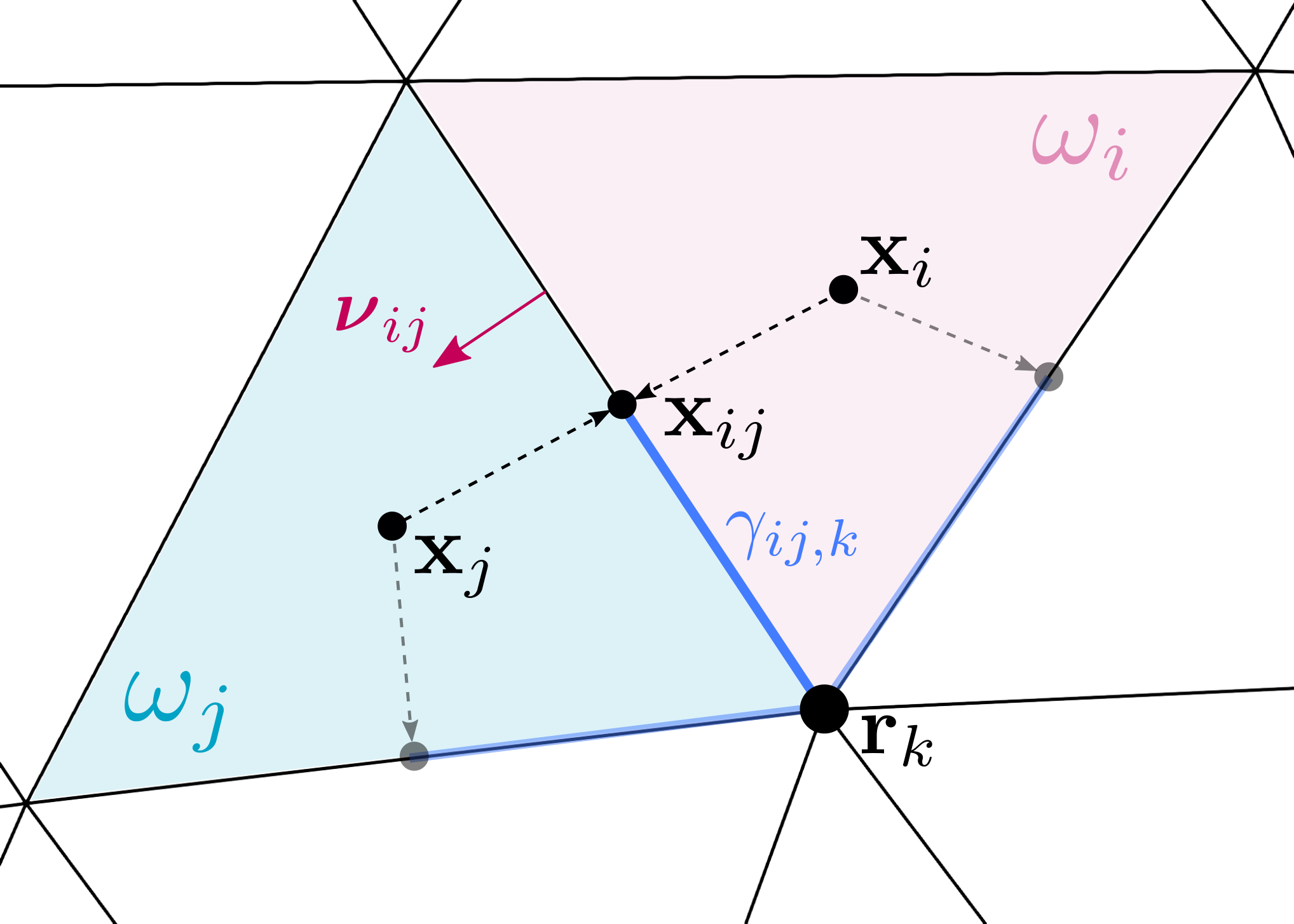
The MPFA method is constructed as follows. First, we endow each $\gamma_{ij,k}$ with a sub-facet pressure $p_{ij,k}$ . With these sub-facet pressures, we compute a discrete gradient $\nabla_{i,k}^{h}p\in\mathbb{R}^{n}$ that satisfies

\displaystyle(\nabla_{i,k}^{h}p)\cdot(\bm{x}_{ij}-\bm{x}_{i})=p_{ij,k}-p_{i},

(3.1)

for all indices $j$ such that $\omega_{j}$ is a neighbor of $\omega_{i}$ that shares vertex $\bm{r}_{k}$ . In order for $\nabla_{i,k}^{h}p$ to be well-defined, we assume that each cell-vertex pair $(i,k)$ has exactly $n$ sub-facets $\gamma_{ij,k}$ . This is true for polygonal grids in 2D and for simplicial and hexahedral grids in 3D.

Second, we formulate the flux continuity condition across each sub-facet $\gamma_{ij,k}$ . Let $K_{i}$ be the conductivity in cell $\omega_{i}$ , then this condition is given by

\displaystyle\bm{\nu}_{ij}\cdot(K_{i}\nabla_{i,k}^{h}p-K_{j}\nabla_{jk}^{h}p)=0.

(3.2)

Third, we fix the vertex index $k$ and collect (3.2) for all neighboring sub-facets $\gamma_{ij,k}$ . Combined with (3.1), this allows us to define the sub-facet pressures as a linear combination of the cell-center pressures. In turn, a substitution in (3.1) effectively eliminates the sub-facet pressures and defines the discrete gradient $\nabla_{i,k}^{h}$ as a linear operator acting on the cell-center pressures.

Finally, we let the discrete gradient define the flux across all facets $\gamma_{ij}$ . Reusing our convention $\bm{\nu}_{i}=\bm{\nu}_{ij}=-\bm{\nu}_{j}$ for $i<j$ , the MPFA method then solves

\displaystyle\sum_{j,k}\int_{\gamma_{ij,k}}(-\bm{\nu}_{i}\cdot(K_{i}\nabla_{i,k}^{h}p))

\displaystyle=\int_{\omega_{i}}f,

\displaystyle\forall\omega_{i}

\displaystyle\in\Omega_{h}.

(3.3)

3.1.2 Multipoint flux mixed finite element method

On simplicial, quadrilateral, and hexahedral elements, the MPFA method has been related to the MFMFE method [42, 28, 40], which is a MFE method with a BDM₁-type space for the velocity and a vertex quadrature rule for the velocity bilinear form $a(\cdot,\cdot)$ . On general polytopal grids, the MPFA method has been formulated as a mimetic finite difference (MFD) method in [33].

We focus first on simplicial grids and the MFMFE formulation of the MPFA method [42]. In Section 5 we discuss smooth quadrilateral and hexahedral grids and comment on the extension to general quadrilateral and hexahedral, as well as general polytopes.

For each $i$ , let $V_{h,i}\times W_{h,i}\subset V_{i}\times W_{i}$ be the BDM₁ pair of spaces on simplices [18], defined as follows. Let $\hat{\omega}$ be the reference triangle or tetrahedron. For each element $\omega\in\Omega_{h}$ there exists an affine bijection mapping $F_{\omega}:\hat{\omega}\rightarrow\omega$ . Denote the Jacobian of $F$ by $D\!F_{\omega}$ and let $J_{\omega}=|\mbox{det}(D\!F_{\omega})|$ . The BDM₁ spaces are defined on the reference element $\hat{\omega}$ as

\hat{V}(\hat{\omega})=P_{1}(\hat{\omega})^{n},\quad\hat{W}(\hat{\omega})=P_{0}(\hat{\omega}),

where $P_{k}$ denotes the space of polynomials of degree at most $k$ . Note that $\hat{\nabla}\cdot\hat{V}(\hat{\omega})=\hat{W}(\hat{\omega})$ and that for all $\hat{\bm{v}}\in\hat{V}(\hat{\omega})$ and for any facet $\hat{\gamma}$ of $\hat{\omega}$ , $\bm{\nu}_{\hat{\gamma}}\cdot\hat{\bm{v}}\in P_{1}(\hat{\gamma})$ . There are two degrees of freedom per facet in two dimensions and three in three dimensions, which can be chosen to be the values of $\bm{\nu}_{\hat{\gamma}}\cdot\hat{\bm{v}}$ at the vertices of $\hat{\gamma}$ .

The BDM₁ spaces on any element $\omega\in\Omega_{h}$ are defined via the transformations

\displaystyle\bm{v}\leftrightarrow\hat{\bm{v}}:\bm{v}

\displaystyle=\frac{1}{J_{\omega}}D\!F_{\omega}\hat{\bm{v}}\circ F_{\omega}^{-1},

\displaystyle w\leftrightarrow\hat{w}:w

\displaystyle=\hat{w}\circ F_{\omega}^{-1},

where the Piola transformation is used for the velocity space. The BDM₁ spaces on $\Omega_{h,i}$ are given by

	$\displaystyle V_{h,i}$	$\displaystyle=\{\bm{v}\in V_{i}\colon$	$\displaystyle\bm{v}\|_{\omega}$	$\displaystyle\leftrightarrow\hat{\bm{v}},$	$\displaystyle\hat{\bm{v}}\in\hat{V}(\hat{\omega}),\forall\omega\in\Omega_{h,i}\},$		(3.4)
	$\displaystyle W_{h,i}$	$\displaystyle=\{w\in W_{i}\colon$	$\displaystyle w\|_{\omega}$	$\displaystyle\leftrightarrow\hat{w},$	$\displaystyle\hat{w}\in\hat{W}(\hat{\omega}),\forall\omega\in\Omega_{h,i}\}.$		(3.4)

The BDM₁ pair is stable for the subproblem defined on $\Omega_{i}$ , such that [18]


$\displaystyle\nabla\cdot V_{h,i}$	$\displaystyle=W_{h,i},$			(3.5a)
$\displaystyle\forall\,w_{h,i}$	$\displaystyle\in W_{h,i},\exists\,0\neq\bm{v}_{h,i}\in V_{h,i}:$	$\displaystyle(\nabla\cdot\bm{v}_{h,i},w_{h,i})_{\Omega_{i}}$	$\displaystyle\gtrsim\\|\bm{v}_{h,i}\\|_{\operatorname{div},\Omega_{i}}\\|w_{h,i}\\|_{\Omega_{i}}.$	(3.5b)

The MFMFE method employs a vertex quadrature rule for the velocity bilinear form $a_{i}(\cdot,\cdot)$ . For any element-wise continuous vector functions $\bm{\phi}$ and $\bm{\psi}$ on $\Omega_{h,i}$ , we denote by

(\bm{\phi},\bm{\psi})_{Q,\Omega_{i}}=\sum_{\omega\in\Omega_{h,i}}(\bm{\phi},\bm{\psi})_{Q,\omega}

the application of the element-wise vertex quadrature rule for computing $(\bm{\phi},\bm{\psi})_{\Omega_{i}}$ . The integration on any element $\omega$ is performed by mapping to the reference element $\hat{\omega}$ . Let $\tilde{\bm{\phi}}$ and $\tilde{\bm{\psi}}$ be the mapped functions on $\hat{\omega}$ , using the standard change of variables. Since $(\bm{\phi},\bm{\psi})_{\omega}=(\tilde{\bm{\phi}},\tilde{\bm{\psi}}J_{\omega})_{\hat{\omega}}$ , we define

(\bm{\phi},\bm{\psi})_{Q,\omega}=\frac{|\hat{\omega}|}{s}\sum_{i=1}^{s}\tilde{\bm{\phi}}(\hat{\bm{r}}_{i})\cdot\tilde{\bm{\psi}}(\hat{\bm{r}}_{i})J_{\omega}(\hat{\bm{r}}_{i})=\frac{|\hat{\omega}|}{s}\sum_{i=1}^{s}\bm{\phi}(\bm{r}_{i})\cdot\bm{\psi}(\bm{r}_{i})J_{\omega}(\hat{\bm{r}}_{i}),

where $s$ is the number of vertices of $\omega$ and $\bm{r}_{i}$ and $\hat{\bm{r}}_{i}$ , $i=1,\ldots,s$ , are the vertices of $\omega$ and $\hat{\omega}$ , respectively. Using this quadrature rule, the velocity bilinear form in the MFMFE is defined as

a^{h}_{i}(\bm{u}_{i},\bm{v}_{i}):=(K^{-1}\bm{u}_{i},\bm{v}_{i})_{Q,\Omega_{i}},\quad a^{h}(\bm{u},\bm{v}):=\sum_{i}a^{h}_{i}(\bm{u}_{i},\bm{v}_{i}).

The quadrature rule localizes the interaction of the velocity degrees of freedom around mesh vertices. This allows for local elimination of the velocity, resulting in a cell-centered finite volume system for the pressure, which is closely related to the MPFA system [4] from Section 3.1.1. However, the quadrature rule introduces a non-conforming term in the numerical error, defined as

\sigma(\bm{\phi},\bm{\psi}):=a(\bm{\phi},\bm{\psi})-a^{h}(\bm{\phi},\bm{\psi}).

(3.6)

A bound on this term is shown in Section 4.

3.2 Interface discretization and coupling

With the subdomain discretizations defined above, we turn to the coupling at the interfaces. Let $V_{h,i}^{0}$ denote the subspace of $V_{h,i}$ with zero normal trace on $\Gamma_{i}$ and let $V_{h,i}^{\Gamma}$ denote the trace space of $V_{h,i}$ on $\Gamma_{i}$ :

	$\displaystyle V_{h,i}^{0}$	$\displaystyle:=\{\bm{v}_{h,i}^{0}\in V_{h,i}:\ (\bm{\nu}_{i}\cdot\bm{v}_{h,i}^{0})\|_{\Gamma_{i}}=0\},$	$\displaystyle\quad V_{h}^{0}$	$\displaystyle:=\bigoplus_{i}V_{h,i}^{0},$		(3.7)
	$\displaystyle V_{h,i}^{\Gamma}$	$\displaystyle:=(\bm{\nu}_{i}\cdot V_{h,i})\|_{\Gamma_{i}},$	$\displaystyle V_{h}^{\Gamma}$	$\displaystyle:=\bigoplus_{i}V_{h,i}^{\Gamma}.$		(3.8)

Let $S_{H}$ be the following null-space:

\displaystyle S_{H,i}:=\{w_{h,i}\in W_{h,i}:\ b_{i}(\bm{v}_{h,i}^{0},w_{h,i})=0,\ \forall\bm{v}_{h,i}^{0}\in V_{h,i}^{0}\},\quad S_{H}:=\bigoplus_{i}S_{H,i},

(3.9)

in which the subscript $H$ refers to the characteristic subdomain size. We note that in this case of Darcy flow, the local spaces can be characterized as

\displaystyle S_{H,i}

\displaystyle=\begin{cases}\mathbb{R},&i\in I_{int},\\ 0,&i\notin I_{int}.\end{cases}

(3.10)

For the interfaces, we introduce a shape-regular tessellation of $\Gamma_{ij}$ , denoted by $\Gamma_{h,ij}$ , with a typical mesh size $h_{\Gamma}$ . Let $\Gamma_{h}=\bigcup_{i<j}\Gamma_{h,ij}$ . Let the discrete interface space $\Lambda_{h,ij}\subset L^{2}(\Gamma_{ij})$ contain continuous or discontinuous piecewise polynomials on $\Gamma_{h,ij}$ of degree $k_{\Lambda}$ and let $\Lambda_{h}=\bigoplus_{i<j}\Lambda_{h,ij}$ .

The method involves incorporating the mortar flux data as Neumann boundary condition for the subdomain problems. Let $\mathcal{Q}_{h}:\Lambda\to V_{h}^{\Gamma}$ be a chosen projection operator and let $\mathcal{Q}_{h,i}:\Lambda\to V_{h,i}^{\Gamma}$ be its restriction to $V_{h,i}^{\Gamma}$ . Following [15], we consider two choices for $\mathcal{Q}_{h,i}$ , described in Sections 3.2.1 and 3.2.2. The extension of the boundary data into the subdomains is described in Section 3.2.3.

3.2.1 Projection onto the normal trace space of the velocity

The first choice is $\mathcal{Q}_{h,i}=\mathcal{Q}_{h,i}^{\flat}$ , where the operator $\mathcal{Q}_{h,i}^{\flat}:\Lambda\to V_{h,i}^{\Gamma}$ is the $L^{2}(\Gamma_{i})$ -orthogonal projection. It is computed for each $i$ by solving the problem: Given $\lambda\in\Lambda$ , find $\mathcal{Q}_{h,i}^{\flat}\lambda\in V_{h,i}^{\Gamma}$ such that

\displaystyle(\lambda_{i}-\mathcal{Q}_{h,i}^{\flat}\lambda,\xi_{h,i})_{\Gamma_{i}}=0,\quad\forall\,\xi_{h,i}

\displaystyle\in V_{h,i}^{\Gamma}.

(3.11)

For the unique solvability of the mortar variable we need for the mortar space on a given interface to be controlled by the normal traces of the neighboring velocity spaces. We make the following assumption.

A1.

The following mortar condition holds:

\displaystyle\forall\mu_{h}\in\Lambda_{h},\quad\|\mu_{h}\|_{\Gamma_{ij}}

\displaystyle\lesssim\|\mathcal{Q}_{h,i}^{\flat}\mu_{h}\|_{\Gamma_{ij}}+\|\mathcal{Q}_{h,j}^{\flat}\mu_{h}\|_{\Gamma_{ij}},\quad\forall\,\Gamma_{ij}.

(3.12)

Remark 3.1.

Assumption A1 for $\mathcal{Q}_{h}^{\flat}$ is the conventional mortar assumption, see e.g. [8, 9], implying that the mortar variable is controlled on each interface by its $L^{2}$ -projection onto the normal trace space on one of the two neighboring subdomains. It has been shown to hold for some very general mesh configurations [9, 35]. In particular, it is easy to satisfy in practice by choosing a sufficiently coarse mortar grid $\Gamma_{h}$ [9].

3.2.2 Projection onto the space of weakly continuous velocities

The second option $\mathcal{Q}_{h,i}=\mathcal{Q}_{h,i}^{\sharp}$ is the orthogonal projection to the space of weakly continuous velocities. Following [8], let the space of weakly continuous fluxes $V_{h,c}$ and the associated trace space $V_{h,c}^{\Gamma}$ be given by


$\displaystyle V_{h,c}$	$\displaystyle:=\left\{\bm{v}_{h}\in\bigoplus_{i}V_{h,i}:\ \sum_{i}(\bm{\nu}_{i}\cdot\bm{v}_{h,i},\mu_{h})_{\Gamma_{i}}=0,\ \forall\mu_{h}\in\Lambda_{h}\right\},$	(3.13a)
$\displaystyle V_{h,c}^{\Gamma}$	$\displaystyle:=\left\{\xi_{h}\in V_{h}^{\Gamma}:\ \sum_{i}(\xi_{h,i},\mu_{h})_{\Gamma_{i}}=0,\ \forall\mu_{h}\in\Lambda_{h}\right\}.$	(3.13b)

We construct the projection $\mathcal{Q}_{h}^{\sharp}:\Lambda\to V_{h}^{\Gamma}$ by solving the following auxiliary problem [8, 15]: Given $\lambda\in\Lambda$ , find $\mathcal{Q}_{h}^{\sharp}\lambda\in V_{h}^{\Gamma}$ and $\chi_{h}\in\Lambda_{h}$ such that


$\displaystyle\sum_{i}(\lambda_{i}-\mathcal{Q}_{h,i}^{\sharp}\lambda-\chi_{h},\xi_{h,i})_{\Gamma_{i}}$	$\displaystyle=0,$	$\displaystyle\forall\xi_{h}$	$\displaystyle\in V_{h}^{\Gamma},$	(3.14a)
$\displaystyle\sum_{i}(\mathcal{Q}_{h,i}^{\sharp}\lambda,\mu_{h})_{\Gamma_{i}}$	$\displaystyle=0,$	$\displaystyle\forall\mu_{h}$	$\displaystyle\in\Lambda_{h}.$	(3.14b)

It is shown in [15, Lemma 3.1] that, if A1 holds, then problem (3.14) has a unique solution. Moreover, it is proved in [15, Lemma 3.2] that $\mathcal{Q}_{h}^{\sharp}\lambda$ is the $L^{2}$ -projection of $\lambda$ onto $V_{h,c}^{\Gamma}$ , satisfying

\displaystyle\sum_{i}(\lambda_{i}-\mathcal{Q}_{h,i}^{\sharp}\lambda,\xi_{h,i})_{\Gamma_{i}}

\displaystyle=0,

\displaystyle\forall\xi_{h}

\displaystyle\in V_{h,c}^{\Gamma}.

For the unique solvability of the mortar variable in the case of $\mathcal{Q}_{h,i}^{\sharp}$ , we make an assumption similar to assumption A1.

A2.

The following mortar condition holds:

\displaystyle\forall\mu_{h}\in\Lambda_{h},\quad\|\mu_{h}\|_{\Gamma_{ij}}

\displaystyle\lesssim\|\mathcal{Q}_{h,i}^{\sharp}\mu_{h}\|_{\Gamma_{ij}}+\|\mathcal{Q}_{h,j}^{\sharp}\mu_{h}\|_{\Gamma_{ij}},\quad\forall\,\Gamma_{ij}.

(3.15)

3.2.3 Discrete extension operator

Next, we define a discrete extension operator $\mathcal{R}_{h,i}:\Lambda\to V_{h,i}$ . For given $\lambda\in\Lambda$ , we consider the following problem: Find $(\mathcal{R}_{h,i}\lambda,p_{h,i}^{\lambda},r_{i})\in V_{h,i}\times W_{h,i}\times S_{H,i}$ such that


$\displaystyle a_{i}^{h}(\mathcal{R}_{h,i}\lambda,\bm{v}_{h,i}^{0})-b_{i}(\bm{v}_{h,i}^{0},p_{h,i}^{\lambda})$	$\displaystyle=0,$	$\displaystyle\forall\bm{v}_{h,i}^{0}\in V_{h,i}^{0},$	(3.16a)
$\displaystyle b_{i}(\mathcal{R}_{h,i}\lambda,w_{h,i})-(r_{i},w_{h,i})_{\Omega_{i}}$	$\displaystyle=0,$	$\displaystyle\forall w_{h,i}\in W_{h,i},$	(3.16b)
$\displaystyle(p_{h,i}^{\lambda},s_{i})_{\Omega_{i}}$	$\displaystyle=0,$	$\displaystyle\forall s_{i}\in S_{H,i},$	(3.16c)
$\displaystyle\bm{\nu}_{i}\cdot\mathcal{R}_{h,i}\lambda$	$\displaystyle=\mathcal{Q}_{h,i}\lambda,$	$\displaystyle\text{ on }\Gamma_{i}.$	(3.16d)

We note that (3.16d) is an essential boundary condition and that, for subdomains adjacent to $\partial\Omega$ , the boundary condition $p_{i}^{\lambda}=0$ on $\partial\Omega_{i}\setminus\Gamma_{i}$ is natural and has been incorporated in (3.16a). The use of the Lagrange multiplier $r_{i}\in S_{H,i}$ ensures that the subproblem is solvable and that the auxiliary variable $p_{h,i}^{\lambda}$ is uniquely defined, i.e. orthogonal to $S_{H,i}$ .

Remark 3.2.

The use of $\mathcal{Q}_{h,i}\lambda=\mathcal{Q}_{h,i}^{\flat}\lambda$ from (3.11) in (3.16d) leads to $\mathcal{R}_{h,i}=\mathcal{R}_{h,i}^{\flat}$ , while $\mathcal{Q}_{h,i}\lambda=\mathcal{Q}_{h,i}^{\sharp}\lambda$ from (3.14) results in $\mathcal{R}_{h,i}=\mathcal{R}_{h,i}^{\sharp}$ . We will present the results that concern both variants by omitting the superscript.

3.3 Flux-mortar MFMFE method

Combining the subdomain and interface discretizations from Sections 3.1 and 3.2, let $\mathcal{R}_{h}:=\bigoplus_{i}\mathcal{R}_{h,i}$ and let the composite spaces $V_{h}$ and $W_{h}$ be defined as

\displaystyle V_{h}

\displaystyle:=\bigoplus_{i}\left(V_{h,i}^{0}\oplus\mathcal{R}_{h,i}\Lambda_{h}\right)=V_{h}^{0}\oplus\mathcal{R}_{h}\Lambda_{h},

\displaystyle W_{h}

\displaystyle:=\bigoplus_{i}W_{h,i}.

(3.17)

We are now ready to define the flux-mortar MFMFE method for problem (2.4): Find $(\bm{u}_{h}^{0},\lambda_{h},p_{h})\in V_{h}^{0}\times\Lambda_{h}\times W_{h}$ such that


$\displaystyle\sum_{i}a^{h}_{i}(\bm{u}_{h,i}^{0}+\mathcal{R}_{h,i}\lambda_{h},\bm{v}_{h,i}^{0})-b_{i}(\bm{v}_{h,i}^{0},p_{h,i})$	$\displaystyle=0,$	$\displaystyle\forall\bm{v}_{h}^{0}\in V_{h}^{0},$	(3.18a)
$\displaystyle\sum_{i}a^{h}_{i}(\bm{u}_{h,i}^{0}+\mathcal{R}_{h,i}\lambda_{h},\mathcal{R}_{h,i}\mu_{h})-b_{i}(\mathcal{R}_{h,i}\mu_{h},p_{h,i})$	$\displaystyle=0,$	$\displaystyle\forall\mu_{h}\in\Lambda_{h},$	(3.18b)
$\displaystyle\sum_{i}b_{i}(\bm{u}_{h,i}^{0}+\mathcal{R}_{h,i}\lambda_{h}),w_{h,i})$	$\displaystyle=(f,w_{h})_{\Omega},$	$\displaystyle\forall w_{h}\in W_{h}.$	(3.18c)

To shorten notation, let $\bm{u}_{h}:=\bm{u}_{h}^{0}+\mathcal{R}_{h}\lambda_{h}$ and $\bm{v}_{h}:=\bm{v}_{h}^{0}+\mathcal{R}_{h}\mu_{h}$ . Then (3.18) can be equivalently written as: Find $\bm{u}_{h}\in V_{h}$ and $p_{h}\in W_{h}$ such that


$\displaystyle a^{h}(\bm{u}_{h},\bm{v}_{h})-b(\bm{v}_{h},p_{h})$	$\displaystyle=0,$	$\displaystyle\forall\bm{v}_{h}$	$\displaystyle\in V_{h},$	(3.19a)
$\displaystyle b(\bm{u}_{h},w_{h})$	$\displaystyle=(f,w_{h})_{\Omega},$	$\displaystyle\forall w_{h}$	$\displaystyle\in W_{h}.$	(3.19b)

Note that the flux-mortar mixed finite element method (3.19) is a non-conforming discretization of the weak formulation (2.4), since in general $V_{h}\not\subset V$ . We further emphasize that the discrete trial and test functions from $V_{h}$ are naturally decomposed into internal and interface degrees of freedom using $\mathcal{R}_{h}$ .

4 Well-posedness and error analysis on simplicial grids

This section concerns the a priori analysis of the flux-mortar MFMFE method proposed in Section 3. We first show that the discrete problem is well-posed in Section 4.1 and then present the error analysis in Section 4.2.

4.1 Well-posedness

We follow the abstract analysis developed in [15, Section 2.4] with modifications to take into account the non-conformity due to the use of the quadrature rule in $a^{h}(\cdot,\cdot)$ . We begin with a variant of [15, Theorem 2.1].

Theorem 4.1.

Assume that problem (3.16) has a unique solution and the resulting extension operator $\mathcal{R}_{h}:\Lambda\to V_{h}$ is continuous, i.e.

\displaystyle\|\mathcal{R}_{h}\lambda\|_{V}

\displaystyle\lesssim\|\lambda\|_{\Lambda},\quad\forall\,\lambda\in\Lambda.

(4.1)

Assume in addition that the following four inequalities hold:


$\displaystyle\forall$	$\displaystyle\bm{u}_{h},\bm{v}_{h}\in V_{h}:$	$\displaystyle a^{h}(\bm{u}_{h},\bm{v}_{h})$	$\displaystyle\lesssim\\|\bm{u}_{h}\\|_{V}\\|\bm{v}_{h}\\|_{V},$	(4.2a)
$\displaystyle\forall$	$\displaystyle\bm{v}_{h}\in V_{h}\text{ and }w_{h}\in W_{h}:$	$\displaystyle b(\bm{v}_{h},w_{h})$	$\displaystyle\lesssim\\|\bm{v}_{h}\\|_{V}\\|w_{h}\\|_{W},$	(4.2b)
$\displaystyle\forall$	$\displaystyle\bm{v}_{h}\in V_{h}\text{ with }b(\bm{v}_{h},w_{h})=0\ \forall w_{h}\in W_{h}:$	$\displaystyle a^{h}(\bm{v}_{h},\bm{v}_{h})$	$\displaystyle\gtrsim\\|\bm{v}_{h}\\|_{V}^{2},$	(4.2c)
$\displaystyle\forall$	$\displaystyle w_{h}\in W_{h},\ \exists\,0\neq\bm{v}_{h}\in V_{h}\text{ such that}:$	$\displaystyle b(\bm{v}_{h},w_{h})$	$\displaystyle\gtrsim\\|\bm{v}_{h}\\|_{V}\\|w_{h}\\|_{W}.$	(4.2d)

Then the discrete problem (3.19) admits a unique solution that satisfies

\displaystyle\|\bm{u}_{h}\|_{V}+\|p_{h}\|_{W}\lesssim\|f\|_{\Omega}.

(4.3)

Proof.

Assumption (4.1) ensures that the space $V_{h}$ is well-defined. The well-posedness of the discrete problem then follows directly from (4.2) and classical saddle point theory [13]. ∎

The verification of the conditions of Theorem 4.1 is presented in the next two lemmas, the first of which is proved in [15, Lemma 3.3].

Lemma 4.1.

Problem (3.16) has a unique solution, which satisfies (4.1).

Lemma 4.2.

The inequalities (4.2) hold.

Proof.

Inequalities (4.2a) and (4.2c) state the continuity and coercivity of the discrete bilinear form $a^{h}(\cdot,\cdot)$ . They have been verified in [42]. We note that, due to (3.5a), (4.2c) is equivalent to $a^{h}(\bm{v}_{h},\bm{v}_{h})\gtrsim\|\bm{v}_{h}\|_{\Omega}^{2}\ \forall\bm{v}_{h}\in V_{h}$ . The continuity of $b(\cdot,\cdot)$ (4.2b) follows easily from its definition, while the inf-sup condition (4.2d) has been established in [15, Lemma 3.4]. ∎

A combination of Theorem 4.1, Lemma 4.1, and Lemma 4.2 implies the following result.

Corollary 4.1.

The discrete problem (3.19) has a unique solution that satisfies (4.3).

The next result, which is a variant of [15, Theorem 2.2], concerns the unique solvability of the mortar variable.

Theorem 4.2.

Let A1 hold in the case of $\mathcal{Q}_{h,i}^{\flat}$ and let A1 and A2 hold in the case of $\mathcal{Q}_{h,i}^{\sharp}$ . Then the mortar solution $\lambda_{h}$ of (3.19) is unique.

Proof.

We utilize the discrete trace inequality

\displaystyle\forall\,i\in I_{\Omega},\quad\|\bm{\nu}_{i}\cdot\bm{v}_{h,i}\|_{\Gamma_{i}}\lesssim h^{-\frac{1}{2}}\|\bm{v}_{h,i}\|_{\Omega_{i}},\quad\forall\bm{v}_{h,i}\in V_{h,i},

(4.4)

which follows from a simple scaling argument. Since $\bm{u}_{h}=\bm{u}_{h}^{0}+\mathcal{R}_{h}\lambda_{h}$ , it holds that $\bm{\nu}_{i}\cdot\bm{u}_{h,i}=\mathcal{Q}_{h,i}\lambda_{h}$ . Then we use A1 or A2 and (4.4) to obtain

\displaystyle\|\lambda_{h}\|_{\Gamma}\lesssim\sum_{i}\|\mathcal{Q}_{h,i}\lambda_{h}\|_{\Gamma_{i}}=\sum_{i}\|\bm{\nu}_{i}\cdot\bm{u}_{h,i}\|_{\Gamma_{i}}\lesssim h^{-\frac{1}{2}}\|\bm{u}_{h}\|_{\Omega}.

The result now follows from (4.3). ∎

4.2 Error analysis

With the well-posedness of the discrete system verified, we continue with the error analysis. We begin by defining suitable interpolation operators in Section 4.2.1, which are used to derive the a priori error estimates in Section 4.2.2.

4.2.1 Interpolation operators

We follow the construction in [15, Section 3.3]. The building blocks in the construction of the interpolant in $V_{h}$ are the canonical subdomain interpolation operators $\Pi_{i}^{V}:V_{i}\cap(H^{\epsilon}(\Omega_{i}))^{n}\to V_{h,i}$ with $\epsilon>0$ , with the properties

	$\displaystyle(\nabla\cdot(\bm{v}_{i}-\Pi_{i}^{V}\bm{v}_{i}),w_{h,i})_{\Omega_{i}}$	$\displaystyle=0,$	$\displaystyle\forall w_{h,i}$	$\displaystyle\in W_{h,i},$		(4.5)
	$\displaystyle(\bm{\nu}_{i}\cdot(\bm{v}_{i}-\Pi_{i}^{V}\bm{v}_{i}),\xi_{h,i})_{\Gamma_{i}}$	$\displaystyle=0,$	$\displaystyle\forall\xi_{h,i}$	$\displaystyle\in V_{h,i}^{\Gamma}.$		(4.6)

The interpolant $\Pi_{i}^{V}$ is locally constructed on each element and satisfies the continuity property

\forall\,\omega\in\Omega_{h,i},\quad\|\Pi_{i}^{V}\bm{v}_{i}\|_{1,\omega}\lesssim\|\bm{v}_{i}\|_{1,\omega},\quad\forall\,\bm{v}_{i}\in H^{1}(\omega).

(4.7)

In addition, let $\Pi_{i}^{W}:L^{2}(\Omega_{i})\to W_{h,i}$ and $\Pi_{ij}^{\Lambda}:L^{2}(\Gamma_{ij})\to\Lambda_{h,ij}$ denote the $L^{2}$ -projection operators onto $W_{h,i}$ and $\Lambda_{h,ij}$ , respectively. Together with the projection $\mathcal{Q}_{h,i}^{\flat}$ onto $V_{h,i}^{\Gamma}$ introduced earlier, we recall the approximation properties [13]:


$\displaystyle\\|\bm{v}-\Pi_{i}^{V}\bm{v}\\|_{\Omega_{i}}$	$\displaystyle\lesssim h^{r_{v}}\\|\bm{v}\\|_{r_{v},\Omega_{i}},$	$\displaystyle 0$	$\displaystyle<r_{v}\leq 2,$	(4.8a)
$\displaystyle\\|\nabla\cdot(\bm{v}-\Pi_{i}^{V}\bm{v})\\|_{\Omega_{i}}$	$\displaystyle\lesssim h^{r_{w}}\\|\nabla\cdot\bm{v}\\|_{r_{w},\Omega_{i}},$	$\displaystyle 0$	$\displaystyle\leq r_{w}\leq 1,$	(4.8b)
$\displaystyle\\|w-\Pi_{i}^{W}w\\|_{\Omega_{i}}$	$\displaystyle\lesssim h^{r_{w}}\\|w\\|_{r_{w},\Omega_{i}},$	$\displaystyle 0$	$\displaystyle\leq r_{w}\leq 1,$	(4.8c)
$\displaystyle\\|\mu-\Pi_{ij}^{\Lambda}\mu\\|_{\Gamma_{ij}}$	$\displaystyle\lesssim h_{\Gamma}^{r_{\Lambda}}\\|\mu\\|_{r_{\Lambda},\Gamma_{ij}},$	$\displaystyle 0$	$\displaystyle\leq r_{\Lambda}\leq k_{\Lambda}+1,$	(4.8d)
$\displaystyle\\|\mu-\mathcal{Q}_{h,i}^{\flat}\mu\\|_{\Gamma_{ij}}$	$\displaystyle\lesssim h^{r_{v}}\\|\mu\\|_{r_{v},\Gamma_{ij}},$	$\displaystyle 0$	$\displaystyle\leq r_{v}\leq 2.$	(4.8e)

Let $\tilde{\Pi}^{V}:\bigoplus_{i}(V_{i}\cap(H^{\epsilon}(\Omega_{i}))^{n})\to\bigoplus_{i}V_{h,i}$ , $\Pi^{W}:W\to W_{h}$ and $\Pi^{\Lambda}:\Lambda\to\Lambda_{h}$ be defined as $\tilde{\Pi}^{V}:=\bigoplus\Pi_{i}^{V}$ , $\Pi^{W}:=\bigoplus_{i}\Pi_{i}^{W}$ and $\Pi^{\Lambda}:=\bigoplus_{i<j}\Pi^{\Lambda}_{ij}$ , respectively.

Next, we introduce the composite interpolant $\Pi^{V}:\overline{V}\to V_{h}$ , where $\overline{V}=\{\bm{v}\in V:\bm{v}|_{\Omega_{i}}\in(H^{\epsilon}(\Omega_{i}))^{n}\text{ and }(\bm{\nu}\cdot\bm{u})|_{\Gamma}\in\Lambda\}$ with $\epsilon>0$ . Given $\bm{u}\in\overline{V}$ with normal trace $\lambda:=(\bm{\nu}\cdot\bm{u})|_{\Gamma}\in\Lambda$ , we define $\Pi^{V}\bm{u}\in V_{h}$ as


		$\displaystyle\Pi_{\flat}^{V}\bm{u}:=\mathcal{R}_{h}^{\flat}\Pi^{\Lambda}\lambda+\tilde{\Pi}^{V}(\bm{u}-\mathcal{R}_{h}^{\flat}\lambda)=\mathcal{R}_{h}^{\flat}(\Pi^{\Lambda}\lambda-\lambda)+\tilde{\Pi}^{V}\bm{u},$		(4.9a)
		$\displaystyle\Pi_{\sharp}^{V}\bm{u}:=\mathcal{R}_{h}^{\sharp}\Pi^{\Lambda}\lambda+\tilde{\Pi}^{V}(\bm{u}-\mathcal{R}_{h}^{\flat}\lambda)=\Pi_{\flat}^{V}\bm{u}-\mathcal{R}_{h}^{\flat}\Pi^{\Lambda}\lambda+\mathcal{R}_{h}^{\sharp}\Pi^{\Lambda}\lambda.$		(4.9b)

We note that (3.16d) for $\mathcal{R}_{h,i}^{\flat}\lambda$ , and (4.6) imply $\bm{\nu}_{i}\cdot\Pi_{i}^{V}(\bm{u}_{i}-\mathcal{R}_{h,i}^{\flat}\lambda)=\mathcal{Q}_{h,i}^{\flat}\lambda-\mathcal{Q}_{h,i}^{\flat}\lambda=0,$ so (4.9) gives $\Pi_{\flat}^{V}\bm{u}\in V_{h}^{\flat}$ and $\Pi_{\sharp}^{V}\bm{u}\in V_{h}^{\sharp}$ . In the following, the use of $\Pi^{V}$ indicates that the result is valid for both choices.

Lemma 4.3 ([15, Lemma 3.7]).

The interpolation operator $\Pi^{V}$ is $b$ -compatible:

\displaystyle b(\bm{u}-\Pi^{V}\bm{u},w_{h})

\displaystyle=0,

\displaystyle\forall\,w_{h}

\displaystyle\in W_{h}.

(4.10)

The approximation properties of the interpolants $\Pi_{\flat}^{V}$ and $\Pi_{\sharp}^{V}$ are given below.

Lemma 4.4 ([15, Lemma 3.8]).

Assuming that $\bm{u}$ has sufficient regularity, then


$\displaystyle\\|\bm{u}-\Pi_{\flat}^{V}\bm{u}\\|_{V}$	$\displaystyle\lesssim h^{r_{v}}\sum_{i}\\|\bm{u}\\|_{r_{v},\Omega_{i}}+h^{r_{w}}\sum_{i}\\|\nabla\cdot\bm{u}\\|_{r_{w},\Omega_{i}}+h_{\Gamma}^{r_{\Lambda}}\sum_{i<j}\\|\lambda\\|_{r_{\Lambda},\Gamma_{ij}},$	(4.11a)
$\displaystyle\\|\bm{u}-\Pi_{\sharp}^{V}\bm{u}\\|_{V}$	$\displaystyle\lesssim h^{r_{v}}\sum_{i}\\|\bm{u}\\|_{r_{v},\Omega_{i}}+h^{r_{w}}\sum_{i}\\|\nabla\cdot\bm{u}\\|_{r_{w},\Omega_{i}}+h_{\Gamma}^{r_{\Lambda}}\sum_{i<j}\\|\lambda\\|_{r_{\Lambda},\Gamma_{ij}}+h^{\tilde{r}_{v}}\sum_{i<j}\\|\lambda\\|_{\tilde{r}_{v},\Gamma_{ij}},$	(4.11b)

for $0<r_{v}\leq 2$ , $0\leq r_{w}\leq 1$ , $0\leq r_{\Lambda}\leq k_{\Lambda}+1$ , and $0\leq\tilde{r}_{v}\leq 2$ .

4.2.2 Error estimate

We proceed with the error estimate in the case of simplicial grids. The following theorem is a variant of [15, Theorem 2.3], accounting for the quadrature error.

Theorem 4.3.

It holds that

\displaystyle\|\bm{u}-\bm{u}_{h}\|_{V}+\|p-p_{h}\|_{W}\lesssim\|\tilde{\Pi}^{V}\bm{u}-\bm{u}\|_{V}+\|\Pi^{V}\bm{u}-\bm{u}\|_{V}+\|\Pi^{W}p-p\|_{W}+\mathcal{E}_{c}+\mathcal{E}_{\sigma},

(4.12)

with $\mathcal{E}_{c}$ the consistency error defined as

\displaystyle\mathcal{E}_{c}:=\sup_{0\neq\bm{v}_{h}\in V_{h}}\frac{a(\bm{u},\bm{v}_{h})-b(\bm{v}_{h},p)}{\|\bm{v}_{h}\|_{V}},

(4.13)

and $\mathcal{E}_{\sigma}$ the quadrature error defined as

\mathcal{E}_{\sigma}:=\sup_{0\neq\bm{v}_{h}\in V_{h}}\frac{\sigma(\tilde{\Pi}^{V}\bm{u},\bm{v}_{h})}{\|\bm{v}_{h}\|_{V}}

(4.14)

with $\sigma(\cdot,\cdot)$ from (3.6).

Proof.

The proof is a modification of the proof of [15, Theorem 2.3], with the main difference being in forming the error equations. In particular, from (3.19) and (2.4b) we obtain the error equations


$\displaystyle a^{h}(\Pi^{V}\bm{u}-\bm{u}_{h},\bm{v}_{h})-b(\bm{v}_{h},\Pi^{W}p-p_{h})$	$\displaystyle=a^{h}(\Pi^{V}\bm{u},\bm{v}_{h})-b(\bm{v}_{h},p),$	(4.15a)
$\displaystyle b(\Pi^{V}\bm{u}-\bm{u}_{h},w_{h})$	$\displaystyle=0,$	(4.15b)

for all $(\bm{v}_{h},w_{h})\in V_{h}\times W_{h}$ , where in (4.15b) we used the $b$ -compatibility of $\Pi^{V}$ (4.10) and the fact that $W_{h}\subset W$ . We manipulate the right hand side of (4.15a) as follows:

\displaystyle\begin{split}a^{h}(\Pi^{V}\bm{u},\bm{v}_{h})-b(\bm{v}_{h},p)&=a^{h}(\Pi^{V}\bm{u}-\tilde{\Pi}^{V}\bm{u},\bm{v}_{h})+a^{h}(\tilde{\Pi}^{V}\bm{u},\bm{v}_{h})-a(\tilde{\Pi}^{V}\bm{u},\bm{v}_{h})\\ &\qquad+a(\tilde{\Pi}^{V}\bm{u}-\bm{u},\bm{v}_{h})+a(\bm{u},\bm{v}_{h})-b(\bm{v}_{h},p).\end{split}

(4.16)

We recognize that the second and third terms on the right in (4.16) form the numerator of the quadrature error $\mathcal{E}_{\sigma}$ from (4.14), and the last two terms form the numerator of the consistency error $\mathcal{E}_{c}$ from (4.13). We next set the test functions in (4.15) as

\displaystyle\bm{v}_{h}:=\Pi^{V}\bm{u}-\bm{u}_{h}-\delta\bm{v}_{h}^{p},\quad w_{h}:=\Pi^{W}p-p_{h}.

(4.17)

Here $\bm{v}_{h}^{p}\in V_{h}$ is constructed, using the inf-sup condition on $b$ (4.2d), to satisfy

\displaystyle b(\bm{v}_{h}^{p},\Pi^{W}p-p_{h})

\displaystyle=\|\Pi^{W}p-p_{h}\|_{W}^{2},

\displaystyle\|\bm{v}_{h}^{p}\|_{V}

\displaystyle\lesssim\|\Pi^{W}p-p_{h}\|_{W},

(4.18)

and $\delta>0$ is a constant to be chosen later. Now (4.15), in combination with (4.16), leads to

\displaystyle\begin{split}&a^{h}(\Pi^{V}\bm{u}-\bm{u}_{h},\Pi^{V}\bm{u}-\bm{u}_{h})+\delta\|\Pi^{W}p-p_{h}\|_{W}^{2}=a^{h}(\Pi^{V}\bm{u}-\bm{u}_{h},\delta\bm{v}_{h}^{p})\\ &\quad+a^{h}(\Pi^{V}\bm{u}-\tilde{\Pi}^{V}\bm{u},\bm{v}_{h})-\sigma(\tilde{\Pi}^{V}\bm{u},\bm{v}_{h})+a(\tilde{\Pi}^{V}\bm{u}-\bm{u},\bm{v}_{h})+\big(a(\bm{u},\bm{v}_{h})-b(\bm{v}_{h},p)\big).\end{split}

(4.19)

For the left-hand side of (4.19), (4.15b) and the coercivity of $a^{h}$ (4.2c) imply


	$\displaystyle\\|\Pi^{V}\bm{u}-\bm{u}_{h}\\|_{V}^{2}\lesssim a^{h}(\Pi^{V}\bm{u}-\bm{u}_{h},\Pi^{V}\bm{u}-\bm{u}_{h}).$		(4.20a)
For the first term on the right in (4.19), using the continuity of $a^{h}$ (4.2a), Young’s inequality with $\epsilon_{1}>0$ , and the bound on $\bm{v}_{h}^{p}$ from (4.18), we obtain

	$\displaystyle a^{h}(\Pi^{V}\bm{u}-\bm{u}_{h},\delta\bm{v}_{h}^{p})$	$\displaystyle\lesssim\frac{\epsilon_{1}}{2}\\|\Pi^{V}\bm{u}-\bm{u}_{h}\\|_{V}^{2}+\frac{1}{2\epsilon_{1}}\delta^{2}\\|\Pi^{W}p-p_{h}\\|_{W}^{2}.$	(4.20b)
Similarly, for the second and fourth terms on the right-hand side of (4.19) we derive, respectively, with $\epsilon_{2}>0$ and $\epsilon_{3}>0$ ,

	$\displaystyle a^{h}(\Pi^{V}\bm{u}-\tilde{\Pi}^{V}\bm{u},\bm{v}_{h})\lesssim\left(\frac{1}{2\epsilon_{2}}+\frac{1}{2}\right)\\|\Pi^{V}\bm{u}-\tilde{\Pi}^{V}\bm{u}\\|_{V}^{2}+\frac{\epsilon_{2}}{2}\\|\Pi^{V}\bm{u}-\bm{u}_{h}\\|_{V}^{2}+\frac{1}{2}\delta^{2}\\|\Pi^{W}p-p_{h}\\|_{W}^{2},$		(4.20c)
and

	$\displaystyle a(\tilde{\Pi}^{V}\bm{u}-\bm{u},\bm{v}_{h})\lesssim\left(\frac{1}{2\epsilon_{3}}+\frac{1}{2}\right)\\|\tilde{\Pi}^{V}\bm{u}-\bm{u}\\|_{V}^{2}+\frac{\epsilon_{3}}{2}\\|\Pi^{V}\bm{u}-\bm{u}_{h}\\|_{V}^{2}+\frac{1}{2}\delta^{2}\\|\Pi^{W}p-p_{h}\\|_{W}^{2}.$		(4.20d)
For the third term on the right in (4.19) we write, with $\epsilon_{4}>0$ ,

	$\displaystyle\begin{split}\sigma(\tilde{\Pi}^{V}\bm{u},\bm{v}_{h})\leq\\|\bm{v}_{h}\\|_{V}\mathcal{E}_{\sigma}\lesssim\frac{\epsilon_{4}}{2}\\|\Pi^{V}\bm{u}-\bm{u}_{h}\\|_{V}^{2}+\frac{1}{2}\delta^{2}\\|\Pi^{W}p-p_{h}\\|_{W}^{2}+\left(\frac{1}{2\epsilon_{4}}+\frac{1}{2}\right)\mathcal{E}_{\sigma}^{2}.\end{split}$		(4.20e)
Finally, for the last two terms in (4.19) we obtain, with $\epsilon_{5}>0$ ,

	$\displaystyle a(\bm{u},\bm{v}_{h})-b(\bm{v}_{h},p)\leq\\|\bm{v}_{h}\\|_{V}\mathcal{E}_{c}\lesssim\frac{\epsilon_{5}}{2}\\|\Pi^{V}\bm{u}-\bm{u}_{h}\\|_{V}^{2}+\frac{1}{2}\delta^{2}\\|\Pi^{W}p-p_{h}\\|_{W}^{2}+\left(\frac{1}{2\epsilon_{5}}+\frac{1}{2}\right)\mathcal{E}_{c}^{2}.$		(4.20f)

Collecting (4.20) and setting all $\epsilon_{i}$ sufficiently small, we arrive at

\displaystyle\|\Pi^{V}\bm{u}-\bm{u}_{h}\|_{V}^{2}+\delta\|\Pi^{W}p-p_{h}\|_{W}^{2}\lesssim\|\tilde{\Pi}^{V}\bm{u}-\bm{u}\|_{V}^{2}+\|\Pi^{V}\bm{u}-\bm{u}\|_{V}^{2}+\delta^{2}\|\Pi^{W}p-p_{h}\|_{W}^{2}+\mathcal{E}_{c}^{2}+\mathcal{E}_{\sigma}^{2}.

We now set $\delta$ sufficiently small to obtain

\displaystyle\|\Pi^{V}\bm{u}-\bm{u}_{h}\|_{V}+\|\Pi^{W}p-p_{h}\|_{W}\lesssim\|\tilde{\Pi}^{V}\bm{u}-\bm{u}\|_{V}+\|\Pi^{V}\bm{u}-\bm{u}\|_{V}+\mathcal{E}_{c}+\mathcal{E}_{\sigma}.

(4.21)

Combining this with the triangle inequality gives us (4.12). ∎

To complete the error estimate, we need to control $\mathcal{E}_{c}$ and $\mathcal{E}_{\sigma}$ . For the consistency error $\mathcal{E}_{c}$ we write, using integration by parts on $\Omega_{i}$ and the boundary condition $p=0$ on $\partial\Omega$ ,

\displaystyle\mathcal{E}_{c}=\sup_{\bm{v}_{h}\in V_{h}}\|\bm{v}_{h}\|_{V}^{-1}\Big((K^{-1}\bm{u},\bm{v}_{h})_{\Omega}-\sum_{i}(p,\nabla\cdot\bm{v}_{h})_{\Omega_{i}}\Big)=\sup_{\bm{v}_{h}\in V_{h}}\|\bm{v}_{h}\|_{V}^{-1}\sum_{i}-(p,\bm{\nu}_{i}\cdot\bm{v}_{h,i})_{\Gamma_{i}},

(4.22)

where we used that $K^{-1}\bm{u}=-\nabla p$ from (2.1). This error has been bounded in [15] for both variants $\mathcal{R}_{h}^{\sharp}$ and $\mathcal{R}_{h}^{\flat}$ . In the case of $\mathcal{R}_{h}=\mathcal{R}_{h}^{\sharp}$ , an additional interpolation operator is utilized. Denoting the discrete subspace consisting of continuous mortar functions by $\Lambda_{h,c}\subset\Lambda_{h}$ , let $\Pi_{c}^{\Lambda}:H^{1}(\Gamma)\to\Lambda_{h,c}$ be the Scott-Zhang interpolant [37] into $\Lambda_{h,c}$ . This interpolant has the approximation property

\displaystyle\|p-\Pi_{c}^{\Lambda}p\|_{s_{\Lambda},\Gamma}\lesssim h_{\Gamma}^{r_{\Lambda}-s_{\Lambda}}\|p\|_{r_{\Lambda},\Gamma},\quad 1\leq r_{\Lambda}\leq k_{\Lambda}+1,\,\,0\leq s_{\Lambda}\leq 1.

(4.23)

We next state the bounds on $\mathcal{E}_{c}$ established in [15].

Lemma 4.5.

Let A1 hold. In the case $\mathcal{R}_{h}=\mathcal{R}_{h}^{\flat}$ , it holds that

\mathcal{E}_{c}\lesssim h^{-\frac{1}{2}}\sum_{i}\|p-\mathcal{Q}_{h,i}^{\flat}p\|_{\Gamma_{i}}.

(4.24)

In the case $\mathcal{R}_{h}=\mathcal{R}_{h}^{\sharp}$ , it holds that

\mathcal{E}_{c}\lesssim\|p-\Pi_{c}^{\Lambda}p\|_{\frac{1}{2},\Gamma}.

(4.25)

Proof.

The bound in the case $\mathcal{R}_{h}=\mathcal{R}_{h}^{\flat}$ is given in [15, (3.34)] and the bound in the case $\mathcal{R}_{h}=\mathcal{R}_{h}^{\sharp}$ is given in [15, (3.33)]. ∎

The quadrature error $\sigma(\cdot,\cdot)$ has been bounded in [42]. In particular, assuming that $K^{-1}|_{\omega}\in W^{1,\infty}(\omega)$ for all elements $\omega$ , it is shown in [42, Lemma 3.5] for each subdomain $\Omega_{i}$ that

\sigma_{i}(\bm{q},\bm{v})\lesssim\sum_{\omega\in\Omega_{h,i}}h\|K^{-1}\|_{1,\infty,\omega}\|\bm{q}\|_{1,\omega}\|\bm{v}\|_{\omega}\quad\forall\,\bm{q},\bm{v}\in V_{h,i},

(4.26)

where $\sigma_{i}:=\sigma|_{\Omega_{i}}$ . We then obtain the following bound.

Lemma 4.6.

Assuming that $K^{-1}|_{\omega}\in W^{1,\infty}(\omega)$ for all elements $\omega$ , it holds that

\mathcal{E}_{\sigma}\lesssim h\sum_{i}\|\bm{u}\|_{1,\Omega_{i}}.

(4.27)

Proof.

The result follows from the definition (4.14) of $\mathcal{E}_{\sigma}$ , bound (4.26), and the continuity of $\tilde{\Pi}$ (4.7). ∎

Combining Theorem 4.3, Lemma 4.5, Lemma 4.6, and the approximation properties (4.8), (4.11), and (4.23), we arrive at the following error estimate.

Theorem 4.4.

Assume that A1 holds and that the solution to (2.3) is sufficiently smooth. Then, in the case $\mathcal{R}_{h}=\mathcal{R}_{h}^{\flat}$ , it holds that

\displaystyle\|\bm{u}-\bm{u}_{h}\|_{V}+\|p-p_{h}\|_{W}\lesssim\ h\sum_{i}\left(\|\bm{u}\|_{1,\Omega_{i}}+\|\nabla\cdot\bm{u}\|_{1,\Omega_{i}}+\|p\|_{1,\Omega_{i}}+\|p\|_{\frac{3}{2},\Gamma_{i}}\right)+h_{\Gamma}^{k_{\Lambda}+1}\sum_{i<j}\|\lambda\|_{k_{\Lambda}+1,\Gamma_{ij}}.

In the case $\mathcal{R}_{h}=\mathcal{R}_{h}^{\sharp}$ , it holds that

	$\displaystyle\\|\bm{u}-\bm{u}_{h}\\|_{V}+\\|p-p_{h}\\|_{W}\lesssim$	$\displaystyle\ h\left(\sum_{i}\left(\\|\bm{u}\\|_{1,\Omega_{i}}+\\|\nabla\cdot\bm{u}\\|_{1,\Omega_{i}}+\\|p\\|_{1,\Omega_{i}}\right)+\sum_{i<j}\\|\lambda\\|_{1,\Gamma_{ij}}\right)$
		$\displaystyle\ +h_{\Gamma}^{k_{\Lambda}+1}\sum_{i<j}\\|\lambda\\|_{k_{\Lambda}+1,\Gamma_{ij}}+h_{\Gamma}^{k_{\Lambda}+\frac{1}{2}}\\|p\\|_{k_{\Lambda}+1,\Gamma}.$

5 Extension to quadrilateral and hexahedral grids

In this section we discuss the flux-mortar MFMFE method for quadrilateral and hexahedral grids. We follow the same steps as in the simplicial case and thus first define the discrete function spaces in Section 5.1, in analogy with Section 3. Second, we show that the discrete system is well-posed in Section 5.2, similar to Section 4.1. Finally, we derive error estimates in Section 5.3.

5.1 Numerical method

For each $i$ , let $V_{h,i}\times W_{h,i}\subset V_{i}\times W_{i}$ be the BDM₁ spaces on quadrilaterals [18] or the enhanced BDDF₁ spaces on hexahedra [28]. On the reference square or cube, the spaces are defined as

\hat{V}(\hat{\omega}):=P_{1}(\hat{\omega})^{n}+S_{n},\quad\hat{W}(\hat{\omega}):=P_{0}(\hat{\omega}),

where the space $S_{2}$ is the span of two divergence-free curl vectors and the space $S_{3}$ is the span of twelve divergence-free curl vectors. Thus, $\text{dim}(\hat{V}(\hat{\omega}))=8$ in $\mathbb{R}^{2}$ and $\text{dim}(\hat{V}(\hat{\omega}))=24$ in $\mathbb{R}^{3}$ . The vector functions in $S_{n}$ are specially chosen, so that $\bm{\nu}_{\hat{\gamma}}\cdot\hat{\bm{v}}\in P_{1}(\hat{\gamma})$ on any facet $\hat{\gamma}$ of $\hat{\omega}$ in $\mathbb{R}^{2}$ and $\bm{\nu}_{\hat{\gamma}}\cdot\hat{\bm{v}}\in Q_{1}(\hat{\gamma})$ on any facet $\hat{\gamma}$ of $\hat{\omega}$ in $\mathbb{R}^{3}$ , where $Q_{1}$ is the space of bilinear functions. As a result, there are two degrees of freedom per facet in two dimensions and four in three dimensions, which can be chosen to be the values of $\bm{\nu}_{\hat{\gamma}}\cdot\hat{\bm{v}}$ at the vertices of $\hat{\gamma}$ . We note the original BDDF₁ space [17] is of dimension 18 and contains only three degrees of freedom per facet. It was enhanced in [28] for the purpose of the MFMFE method. The spaces $V_{h,i}$ and $W_{h,i}$ are defined as in (3.4).

Here we focus on $h^{2}$ -parallelograms or $h^{2}$ -parallelepipeds and a symmetric quadrature rule, which have been studied in [42, 28]. In two dimensions, an element $\omega$ is an $h^{2}$ -parallelogram if

|\vec{a}-\vec{b}|_{\mathbb{R}^{2}}\lesssim h^{2},

where $\vec{a}$ and $\vec{b}$ are any two opposite facets of $\omega$ and $|\cdot|_{\mathbb{R}^{2}}$ is the Euclidean vector norm. In three dimensions, an element $\omega$ is an $h^{2}$ -parallelepiped if all of its facets are $h^{2}$ -parallelograms.

Remark 5.1.

The developments in this section can be extended to general quadrilaterals and hexahedra using a non-symmetric quadrature rule and employing the techniques developed in [31, 40], as well as to general polytopes using the MFD formulation of the MPFA method and the theory developed in [33].

The main difference from the case of simplicial elements is that the space $S_{n}$ contains quadratic functions. As a result, the quadrature error bound (4.26) no longer holds. In order to obtain a similar bound, one needs to restrict the second argument $\bm{v}$ in $\sigma_{i}(\bm{q},\bm{v})$ to be at most piecewise linear. To this end, following [42, 28, 41], we consider the lowest order Raviart-Thomas ( $\text{RT}_{0}$ ) spaces, which are defined on the reference square or cube as

\hat{V}^{\text{RT}}(\hat{\omega}):=P_{0}(\hat{\omega})^{n}+(\alpha_{1}x_{1},\ldots,\alpha_{n}x_{n})^{T},\quad\hat{W}^{\text{RT}}(\hat{\omega})=W(\hat{\omega})=P_{0}(\hat{\omega}),

where $\alpha_{i}$ are real numbers. The spaces $V_{h,i}^{\text{RT}}$ and $W_{h,i}^{\text{RT}}$ are defined as in (3.4).

Let $V_{h}^{\Gamma,\text{RT}}$ , $V_{h,c}^{\text{RT}}$ , and $V_{h,c}^{\Gamma,\text{RT}}$ be the $\text{RT}_{0}$ counterparts of the spaces $V_{h}^{\Gamma}$ , $V_{h,c}$ , and $V_{h,c}^{\Gamma}$ defined in (3.8), (3.13a), and (3.13b), respectively. We modify the projection operator $\mathcal{Q}_{h,i}$ as follows. In the first option we set $\mathcal{Q}_{h,i}=\mathcal{Q}_{h,i}^{\flat,\text{RT}}$ , where $\mathcal{Q}_{h,i}^{\flat,\text{RT}}:\Lambda\to V_{h,i}^{\Gamma,\text{RT}}$ is the $L^{2}(\Gamma_{i})$ -orthogonal projection satisfying

\displaystyle(\lambda_{i}-\mathcal{Q}_{h,i}^{\flat,\text{RT}}\lambda,\xi_{h,i})_{\Gamma_{i}}=0,\quad\forall\,\xi_{h,i}

\displaystyle\in V_{h,i}^{\Gamma,\text{RT}}.

The mortar condition A1 is replaced by

{}^{\text{RT}}

The following mortar condition holds:

\displaystyle\forall\mu_{h}\in\Lambda_{h},\quad\|\mu_{h}\|_{\Gamma_{ij}}

\displaystyle\lesssim\|\mathcal{Q}_{h,i}^{\flat,\text{RT}}\mu_{h}\|_{\Gamma_{ij}}+\|\mathcal{Q}_{h,j}^{\flat,\text{RT}}\mu_{h}\|_{\Gamma_{ij}},\quad\forall\,\Gamma_{ij}.

(5.1)

In the second option we set $\mathcal{Q}_{h,i}=\mathcal{Q}_{h,i}^{\sharp,\text{RT}}$ , where $\mathcal{Q}_{h}^{\sharp,\text{RT}}:\Lambda\to V_{h,c}^{\Gamma,\text{RT}}$ is the $L^{2}$ -projection of $\lambda$ onto $V_{h,c}^{\Gamma,\text{RT}}$ , satisfying

\displaystyle\sum_{i}(\lambda_{i}-\mathcal{Q}_{h,i}^{\sharp,\text{RT}}\lambda,\xi_{h,i})_{\Gamma_{i}}=0,\quad\forall\xi_{h}\in V_{h,c}^{\Gamma,\text{RT}}.

The mortar condition A2 is replaced by

{}^{\text{RT}}

The following mortar condition holds:

\displaystyle\forall\mu_{h}\in\Lambda_{h},\quad\|\mu_{h}\|_{\Gamma_{ij}}

\displaystyle\lesssim\|\mathcal{Q}_{h,i}^{\sharp,\text{RT}}\mu_{h}\|_{\Gamma_{ij}}+\|\mathcal{Q}_{h,j}^{\sharp,\text{RT}}\mu_{h}\|_{\Gamma_{ij}},\quad\forall\,\Gamma_{ij}.

(5.2)

The above modifications affect the discrete extension operator $\mathcal{R}_{h,i}$ defined in (3.16), cf. (3.16d), and consequently the definition of the discrete velocity space $V_{h}$ , cf. (3.17). With these modifications, the flux-mortar MFMFE method on quadrilateral and hexahedral grids is defined as in (3.19).

5.2 Well-posedness

Similar to Corollary 4.1, the well-posedness of the discrete problem follows directly.

Corollary 5.1.

The discrete problem (3.19) in the case of $h^{2}$ -parallelograms or $h^{2}$ -parallelepipeds has a unique solution that satisfies (4.3).

Proof.

The statement follows from Theorem 4.1. In particular, Lemma 4.1 still holds in this case. Inequalities (4.2a) and (4.2c) for these types of elements have been verified in [42, 28]. The continuity of $b(\cdot,\cdot)$ (4.2b) and the inf-sup condition (4.2d) follow as in the case of simplices. ∎

The proof of the following theorem is the same as the proof of Theorem 4.2.

Theorem 5.1.

Let A1 RT hold in the case of $\mathcal{Q}_{h,i}^{\flat,\text{RT}}$ and let A1 RT and A2 RT hold in the case of $\mathcal{Q}_{h,i}^{\sharp,\text{RT}}$ . Then the mortar solution $\lambda_{h}$ of (3.19) is unique.

5.3 Error analysis

In this section, we follow the same steps as in Section 4.2 to present the a priori error analysis. Thus, we first define suitable interpolation operators in Section 5.3.1 and present the error estimates in Section 5.3.2.

5.3.1 Interpolation operators

The definition of the composite interpolant $\Pi^{V}:\overline{V}\to V_{h}$ is modified from (4.9) to


		$\displaystyle\Pi_{\flat}^{V}\bm{u}:=\mathcal{R}_{h}^{\flat,\text{RT}}\Pi^{\Lambda}\lambda+\tilde{\Pi}^{V}(\bm{u}-\mathcal{R}_{h}^{\flat}\lambda)=\mathcal{R}_{h}^{\flat,\text{RT}}(\Pi^{\Lambda}\lambda-\lambda)+\mathcal{R}_{h}^{\flat,\text{RT}}\lambda-\mathcal{R}_{h}^{\flat}\lambda+\tilde{\Pi}^{V}\bm{u},$		(5.3a)
		$\displaystyle\Pi_{\sharp}^{V}\bm{u}:=\mathcal{R}_{h}^{\sharp,\text{RT}}\Pi^{\Lambda}\lambda+\tilde{\Pi}^{V}(\bm{u}-\mathcal{R}_{h}^{\flat}\lambda)=\Pi_{\flat}^{V}\bm{u}-\mathcal{R}_{h}^{\flat,\text{RT}}\Pi^{\Lambda}\lambda+\mathcal{R}_{h}^{\sharp,\text{RT}}\Pi^{\Lambda}\lambda.$		(5.3b)

As in (4.9), $\Pi_{i}^{V}(\bm{u}_{i}-\mathcal{R}_{h,i}^{\flat}\lambda)\in V_{i}^{0}$ , so (5.3) gives $\Pi_{\flat}^{V}\bm{u}\in V_{h}^{\flat}$ and $\Pi_{\sharp}^{V}\bm{u}\in V_{h}^{\sharp}$ . We next note that Lemma 4.3 still holds. We also have the following approximation properties.

Lemma 5.1.

Assuming that $\bm{u}$ has sufficient regularity, then

\displaystyle\|\bm{u}-\Pi^{V}\bm{u}\|_{V}

\displaystyle\lesssim h^{r_{v}}\sum_{i}\|\bm{u}\|_{r_{v},\Omega_{i}}+h^{r_{w}}\sum_{i}\|\nabla\cdot\bm{u}\|_{r_{w},\Omega_{i}}+h_{\Gamma}^{r_{\Lambda}}\sum_{i<j}\|\lambda\|_{r_{\Lambda},\Gamma_{ij}}+h^{\tilde{r}_{v}}\sum_{i<j}\|\lambda\|_{\tilde{r}_{v},\Gamma_{ij}},

(5.4)

for $0<r_{v}\leq 2$ , $0\leq r_{w}\leq 1$ , $0\leq r_{\Lambda}\leq k_{\Lambda}+1$ , and $0\leq\tilde{r}_{v}\leq 1$ .

Proof.

Compared to the second expression in (4.9a), there is an additional term $\mathcal{R}_{h}^{\flat,\text{RT}}\lambda-\mathcal{R}_{h}^{\flat}\lambda$ in (5.3a). Since this is the discrete extension (3.16) with boundary data $\mathcal{Q}_{h,i}^{\flat,\text{RT}}\lambda-\mathcal{Q}_{h,i}^{\flat}\lambda$ in (3.16d), the continuity of $\mathcal{R}_{h,i}$ (4.1), cf. Lemma 4.1, implies that $\|\mathcal{R}_{h,i}^{\flat,\text{RT}}\lambda-\mathcal{R}_{h,i}^{\flat}\lambda\|_{\Omega_{i}}\lesssim\|\mathcal{Q}_{h,i}^{\flat,\text{RT}}\lambda-\mathcal{Q}_{h,i}^{\flat}\lambda\|_{\Omega_{i}}$ , which leads to the last term in (5.4). The rest of the terms are bounded as in the proof of Lemma 4.4, cf. [15, Lemma 3.8]. We note that both variants of $\Pi^{V}\bm{u}$ now have the same approximation properties. We also remark that, compared to the range of the index $\tilde{r}_{v}$ in (4.11b), we now have $0\leq\tilde{r}_{v}\leq 1$ . The reason for the change is that the space $V_{h,i}^{\Gamma,\text{RT}}$ contains piecewise constant functions, rather than piecewise linears, as is the case for $V_{h,i}^{\Gamma}$ . ∎

Let $\Pi_{i}^{\text{RT}}:V_{i}\cap(H^{\epsilon}(\Omega_{i}))^{n}\to V_{h,i}^{\text{RT}}$ be the canonical mixed interpolant of $\text{RT}_{0}$ , with properties


$\displaystyle(\nabla\cdot(\bm{v}_{i}-\Pi_{i}^{\text{RT}}\bm{v}_{i}),w_{h,i})_{\Omega_{i}}$	$\displaystyle=0,$	$\displaystyle\forall\,w_{h,i}$	$\displaystyle\in W_{h,i},$	(5.5a)
$\displaystyle(\bm{\nu}_{i}\cdot(\bm{v}_{i}-\Pi_{i}^{\text{RT}}\bm{v}_{i}),\xi_{h,i})_{\Gamma_{i}}$	$\displaystyle=0,$	$\displaystyle\forall\,\xi_{h,i}$	$\displaystyle\in V_{h,i}^{\Gamma,\text{RT}},$	(5.5b)
$\displaystyle\\|\Pi_{i}^{\text{RT}}\bm{v}_{i}\\|_{1,\omega}$	$\displaystyle\lesssim\\|\bm{v}_{i}\\|_{1,\omega},$	$\displaystyle\forall\,\bm{v}_{i}$	$\displaystyle\in H^{1}(\omega).$	(5.5c)

Moreover, $\Pi_{i}^{\text{RT}}$ preserves the divergence and is continuous:


$\displaystyle\nabla\cdot\Pi_{i}^{\text{RT}}\bm{v}_{h,i}$	$\displaystyle=\nabla\cdot\bm{v}_{h,i},$	$\displaystyle\quad\forall\,\bm{v}_{h,i}$	$\displaystyle\in V_{h,i},$	(5.6a)
$\displaystyle\\|\Pi_{i}^{\text{RT}}\bm{v}_{h,i}\\|_{\omega}$	$\displaystyle\lesssim\\|\bm{v}_{h,i}\\|_{\omega},$	$\displaystyle\quad\forall\,\bm{v}_{h,i}$	$\displaystyle\in V_{h,i}.$	(5.6b)

5.3.2 Error estimate

Using the interpolation operators from Section 5.3.1, we arrive at the following error estimate.

Theorem 5.2.

In the case of $h^{2}$ -parallelograms or $h^{2}$ -parallelepipeds, it holds that

\displaystyle\|\bm{u}-\bm{u}_{h}\|_{V}+\|p-p_{h}\|_{W}\lesssim\|\tilde{\Pi}^{V}\bm{u}-\bm{u}\|_{V}+\|\Pi^{V}\bm{u}-\bm{u}\|_{V}+\|\Pi^{W}p-p\|_{W}+\mathcal{E}_{c}^{\text{RT}}+\mathcal{E}_{\sigma}^{\text{RT}}+\mathcal{E}_{h}^{\text{RT}},

(5.7)

where


		$\displaystyle\mathcal{E}_{c}^{\text{RT}}:=\sup_{0\neq\bm{v}_{h}\in V_{h}}\frac{a(\bm{u},\Pi^{\text{RT}}\bm{v}_{h})-b(\Pi^{\text{RT}}\bm{v}_{h},p)}{\\|\bm{v}_{h}\\|_{V}},$		(5.8a)
		$\displaystyle\mathcal{E}_{\sigma}^{\text{RT}}:=\sup_{0\neq\bm{v}_{h}\in V_{h}}\frac{\sigma(\tilde{\Pi}^{V}\bm{u},\Pi^{\text{RT}}\bm{v}_{h})}{\\|\bm{v}_{h}\\|_{V}},$		(5.8b)
		$\displaystyle\mathcal{E}_{h}^{\text{RT}}:=\sup_{0\neq\bm{v}_{h}\in V_{h}}\frac{a^{h}(\tilde{\Pi}^{V}\bm{u},\bm{v}_{h}-\Pi^{\text{RT}}\bm{v}_{h})}{\\|\bm{v}_{h}\\|_{V}}.$		(5.8c)

Proof.

We start with the error equations (4.15) from the proof of Theorem 4.3, but now we manipulate the right hand side of (4.15a) in a different way:

\displaystyle\begin{split}&a^{h}(\Pi^{V}\bm{u},\bm{v}_{h})-b(\bm{v}_{h},p)=a^{h}(\Pi^{V}\bm{u}-\tilde{\Pi}^{V}\bm{u},\bm{v}_{h})+a^{h}(\tilde{\Pi}^{V}\bm{u},\bm{v}_{h}-\Pi^{\text{RT}}\bm{v}_{h})\\ &\qquad+a^{h}(\tilde{\Pi}^{V}\bm{u},\Pi^{\text{RT}}\bm{v}_{h})-a(\tilde{\Pi}^{V}\bm{u},\Pi^{\text{RT}}\bm{v}_{h})+a(\tilde{\Pi}^{V}\bm{u}-\bm{u},\Pi^{\text{RT}}\bm{v}_{h})+a(\bm{u},\Pi^{\text{RT}}\bm{v}_{h})-b(\Pi^{\text{RT}}\bm{v}_{h},p),\end{split}

where we used (5.6a) for the last term. We recognize that the second term on the right forms the numerator of the error $\mathcal{E}_{h}^{\text{RT}}$ from (5.8c), the third and fourth terms form the numerator of the quadrature error $\mathcal{E}_{\sigma}^{\text{RT}}$ from (5.8b), and the last two terms form the numerator of the consistency error $\mathcal{E}_{c}^{\text{RT}}$ from (5.8a). The rest of the proof follows the proof of Theorem 4.3. ∎

We proceed with the bounds of the three error terms on the right in (5.7). For $\mathcal{E}_{c}^{\text{RT}}$ , recalling (4.22), we write

\displaystyle\mathcal{E}_{c}^{\text{RT}}=\sup_{\bm{v}_{h}\in V_{h}}\|\bm{v}_{h}\|_{V}^{-1}\sum_{i}-(p,\bm{\nu}_{i}\cdot\Pi_{i}^{\text{RT}}\bm{v}_{h,i})_{\Gamma_{i}}=\sup_{\bm{v}_{h}\in V_{h}}\|\bm{v}_{h}\|_{V}^{-1}\sum_{i}-(p,\bm{\nu}_{i}\cdot\bm{v}_{h,i})_{\Gamma_{i}},

(5.9)

where we used that $\Pi_{i}^{\text{RT}}$ satisfies (5.5b) and that by construction $\bm{v}_{h,i}\in V_{h,i}^{\Gamma,\text{RT}}$ . Therefore, the arguments leading to (3.33) and (3.34) in [15] also hold in this case, leading the following result, similar to Lemma 4.5.

Lemma 5.2.

Let A1 RT hold. In the case $\mathcal{R}_{h}=\mathcal{R}_{h}^{\flat,\text{RT}}$ , it holds that

\mathcal{E}_{c}^{\text{RT}}\lesssim h^{-\frac{1}{2}}\sum_{i}\|p-\mathcal{Q}_{h,i}^{\flat,\text{RT}}p\|_{\Gamma_{i}}.

(5.10)

In the case $\mathcal{R}_{h}=\mathcal{R}_{h}^{\sharp,\text{RT}}$ , it holds that

\mathcal{E}_{c}^{\text{RT}}\lesssim\|p-\Pi_{c}^{\Lambda}p\|_{\frac{1}{2},\Gamma}.

(5.11)

For the quadrature error, we refer to [42, Lemma 3.5] for $h^{2}$ -parallelograms and [28, Lemma 3.8] for $h^{2}$ -parallelepipeds, where it is shown that

\sigma_{i}(\bm{q},\bm{v})\lesssim\sum_{\omega\in\Omega_{h,i}}h\|K^{-1}\|_{1,\infty,\omega}\|\bm{q}\|_{1,\omega}\|\bm{v}\|_{\omega}\quad\forall\,\bm{q}\in V_{h,i},\bm{v}\in V_{h,i}^{\text{RT}}.

(5.12)

Lemma 5.3.

Assuming that $K^{-1}|_{\omega}\in W^{1,\infty}(\omega)$ for all elements $\omega$ , it holds that

\mathcal{E}_{\sigma}^{\text{RT}}\lesssim h\sum_{i}\|\bm{u}\|_{1,\Omega_{i}}.

(5.13)

Proof.

The result follows from the definition (5.8b) of $\mathcal{E}_{\sigma}^{\text{RT}}$ , bound (5.12), and the continuity properties (4.7) and (5.6b). ∎

Finally, $\mathcal{E}_{h}^{\text{RT}}$ has been bounded in [42, Lemma 3.3] for $h^{2}$ -parallelograms and [28, Lemma 3.7] for $h^{2}$ -parallelepipeds.

Lemma 5.4.

Assuming that $K^{-1}|_{\omega}\in W^{1,\infty}(\omega)$ for all elements $\omega$ , it holds that

\mathcal{E}_{h}^{\text{RT}}\lesssim h\sum_{i}\|\bm{u}\|_{1,\Omega_{i}}.

(5.14)

Combining Theorem 5.2, Lemma 5.2, Lemma 5.3, Lemma 5.4, and the approximation properties (4.8), (4.11), and (4.23), we arrive at the main error estimate.

Theorem 5.3.

Assume that A1 RT holds, that the solution to (2.3) is sufficiently smooth, and that the grids consist of $h^{2}$ -parallelograms or $h^{2}$ -parallelepipeds. Then, in the case $\mathcal{R}_{h}=\mathcal{R}_{h}^{\flat,\text{RT}}$ , it holds that

	$\displaystyle\\|\bm{u}-\bm{u}_{h}\\|_{V}+\\|p-p_{h}\\|_{W}\lesssim$	$\displaystyle\ h\left(\sum_{i}\left(\\|\bm{u}\\|_{1,\Omega_{i}}+\\|\nabla\cdot\bm{u}\\|_{1,\Omega_{i}}+\\|p\\|_{1,\Omega_{i}}\right)+\sum_{i<j}\\|\lambda\\|_{1,\Gamma_{ij}}\right)$
		$\displaystyle+h_{\Gamma}^{k_{\Lambda}+1}\sum_{i<j}\\|\lambda\\|_{k_{\Lambda}+1,\Gamma_{ij}}+\sum_{i}h^{\frac{1}{2}}\\|p\\|_{1,\Gamma_{i}}.$

In the case $\mathcal{R}_{h}=\mathcal{R}_{h}^{\sharp,\text{RT}}$ , it holds that

	$\displaystyle\\|\bm{u}-\bm{u}_{h}\\|_{V}+\\|p-p_{h}\\|_{W}\lesssim$	$\displaystyle\ h\left(\sum_{i}\left(\\|\bm{u}\\|_{1,\Omega_{i}}+\\|\nabla\cdot\bm{u}\\|_{1,\Omega_{i}}+\\|p\\|_{1,\Omega_{i}}\right)+\sum_{i<j}\\|\lambda\\|_{1,\Gamma_{ij}}\right)$
		$\displaystyle+h_{\Gamma}^{k_{\Lambda}+1}\sum_{i<j}\\|\lambda\\|_{k_{\Lambda}+1,\Gamma_{ij}}+h_{\Gamma}^{k_{\Lambda}+\frac{1}{2}}\\|p\\|_{k_{\Lambda}+1,\Gamma}.$

6 Non-overlapping domain decomposition

In this section we present a non-overlapping domain decomposition algorithm for the solution of the algebraic system of the flux-mortar MFMFE method. It is based on reduction to an interface problem for the flux-mortar variable. We further develop a preconditioner for the resulting interface problem. The general domain decomposition methodology is based on techniques developed in [27]. We refer to [15, Section 2.5] for a detailed presentation and analysis of the method.

6.1 Reduction to an interface problem

We assume that A1 hold in the case of $\mathcal{Q}_{h,i}^{\flat}$ and that A1 and A2 hold in the case of $\mathcal{Q}_{h,i}^{\sharp}$ , in which case the mortar solution $\lambda_{h}$ of (3.19) is unique, see Theorem 4.2.

In the solution process we utilize the extension $\tilde{\mathcal{R}}_{h}\mu\in\bigoplus_{i}V_{h,i}$ with $\Tr\tilde{\mathcal{R}}_{h,i}\mu=\mathcal{Q}_{h,i}\mu$ on $\Gamma_{i}$ , such that all of its degrees of freedom not associated with $\Gamma_{i}$ are equal to zero. We also utilize the orthogonal decomposition $\Lambda_{h}=\Lambda_{h}^{0}\oplus\overline{\Lambda}_{h}$ , where

\displaystyle\Lambda_{h}^{0}:=\{\mu\in\Lambda_{h}:\ b(\tilde{\mathcal{R}}_{h}\mu,s)=0,\ \forall s\in S_{H}\}.

(6.1)

Let $B:\Lambda_{h}\to S_{H}^{\prime}$ be defined as: $\forall\,\mu\in\Lambda_{h},\langle B\mu,s\rangle:=b(\tilde{\mathcal{R}}_{h}\mu,s)\ \forall\,s\in S_{H}$ .

The solution method has the following five steps.

1.

Find $\overline{\lambda}_{f}\in\overline{\Lambda}_{h}$ such that

$\displaystyle b(\tilde{\mathcal{R}}_{h}\overline{\lambda}_{f},s)=\langle f,s\rangle,\quad\forall s$ $\displaystyle\in S_{H}.$ (6.2)

This is a global coarse problem $B\overline{\lambda}_{f}=\overline{f}$ in $S_{H}^{\prime}$ , which captures the influence of $f$ in (3.18c) with respect to the space $S_{H}$ , c.f. (3.10).

Use $\overline{\lambda}_{f}$ to solve independent, local subproblems to satisfy (3.18a) and capture the remaining influence of $f$ in (3.18c): Find $(\bm{u}_{f}^{0},p_{f}^{0},r_{f})\in V_{h}^{0}\times W_{h}\times S_{H}$ such that


$\displaystyle a^{h}(\bm{u}_{f}^{0},\bm{v}^{0})-b(\bm{v}^{0},p_{f}^{0})$	$\displaystyle=-a^{h}(\tilde{\mathcal{R}}_{h}\overline{\lambda}_{f},\bm{v}^{0})+\langle g,\bm{v}^{0}\rangle,$	$\displaystyle\forall\bm{v}^{0}$	$\displaystyle\in V_{h}^{0},$	(6.3a)
$\displaystyle b(\bm{u}_{f}^{0},w)-(r_{f},w)_{\Omega}$	$\displaystyle=-b(\tilde{\mathcal{R}}_{h}\overline{\lambda}_{f},w)+\langle f,w\rangle,$	$\displaystyle\forall w$	$\displaystyle\in W_{h},$	(6.3b)
$\displaystyle(p_{f}^{0},s)_{\Omega}$	$\displaystyle=0,$	$\displaystyle\forall s$	$\displaystyle\in S_{H}.$	(6.3c)

We note that setting $w=r_{f}\in S_{H}$ and using (6.2) with (3.9) implies that $r_{f}=0$ . Therefore, the variable $\bm{u}_{f}:=\bm{u}_{f}^{0}+\tilde{\mathcal{R}}_{h}\overline{\lambda}_{f}$ satisfies (3.18c). In addition, $\bm{u}_{f}$ and $p_{f}^{0}$ satisfy (3.18a).

Satisfy the continuity equation (3.18b) in $\Lambda_{h}^{0}$ by solving the interface problem: Find $\lambda^{0}\in\Lambda_{h}^{0}$ such that

\displaystyle a^{h}(\mathcal{R}_{h}\lambda^{0},\tilde{\mathcal{R}}_{h}\mu^{0})-b(\tilde{\mathcal{R}}_{h}\mu^{0},p^{\lambda^{0}})

\displaystyle=-a^{h}(\bm{u}_{f},\tilde{\mathcal{R}}_{h}\mu^{0})+b(\tilde{\mathcal{R}}_{h}\mu^{0},p_{f}^{0}),

\displaystyle\forall\mu^{0}\in\Lambda_{h}^{0},

(6.4)

where $(\mathcal{R}_{h}\lambda^{0},p^{\lambda^{0}})$ solve the discrete extension problem (3.16).

Guarantee that (3.18b) holds in $\overline{\Lambda}_{h}$ and obtain the correct variable $p$ : Find $\overline{p}_{\lambda}\in S_{H}$ such that

\displaystyle b(\tilde{\mathcal{R}}_{h}\overline{\mu},\overline{p}_{\lambda})

\displaystyle=a^{h}(\bm{u}_{f}+\mathcal{R}_{h}\lambda^{0},\tilde{\mathcal{R}}_{h}\overline{\mu})-b(\tilde{\mathcal{R}}_{h}\overline{\mu},p^{\lambda^{0}}+p_{f}^{0}),

\displaystyle\forall\overline{\mu}\in\overline{\Lambda}_{h},

(6.5)

which is a coarse grid problem $B^{T}\overline{p}_{\lambda}=\overline{g}$ in $\overline{\Lambda}_{h}^{\prime}$ .

Construct:

\displaystyle\bm{u}:=\bm{u}_{f}+\mathcal{R}_{h}\lambda^{0}=\bm{u}_{f}^{0}+\mathcal{R}_{h}\lambda^{0}+\tilde{\mathcal{R}}_{h}\overline{\lambda}_{f},\quad p:=p_{f}^{0}+p^{\lambda^{0}}+\overline{p}_{\lambda},\quad\lambda=\lambda^{0}+\overline{\lambda}_{f}.

(6.6)

It is easy to check that $(\bm{u},p)\in V_{h}\times W_{h}$ solve (3.19).

The interface problem (6.4) is of the type $a_{\Gamma}(\lambda^{0},\mu^{0})=\langle r,\mu^{0}\rangle$ , where $a_{\Gamma}(\lambda^{0},\mu^{0}):=a^{h}(\mathcal{R}_{h}\lambda^{0},\tilde{\mathcal{R}}_{h}\mu^{0})-b(\tilde{\mathcal{R}}_{h}\mu^{0},p^{\lambda^{0}})$ . It is shown in [15, Lemma 2.5] that $a_{\Gamma}(\lambda^{0},\mu^{0})=a^{h}(\mathcal{R}_{h}\lambda^{0},\tilde{\mathcal{R}}_{h}\mu^{0})$ and that it is symmetric and positive definite on $\Lambda_{h}^{0}\times\Lambda_{h}^{0}$ . Therefore (6.4) can be solved using a Krylov space iterative method such as the Conjugate Gradient or GMRES.

6.2 Preconditioner for the interface problem

To speed up the convergence of the iterative interface solver for (6.4) we develop a Dirichlet–Dirichlet type preconditioner, cf. the FETI Dirichlet preconditioner for the primal formulation [38], which requires solving local Dirichlet problems at each iteration: Given $g\in L^{2}(\Gamma)$ , for $i=1,\ldots,n_{\Omega}$ , find $(\bm{u}_{h,i}^{g},p_{h,i}^{g})\in V_{h,i}\times W_{h,i}$ such that


$\displaystyle a_{i}^{h}(\bm{u}_{h,i}^{g},\bm{v}_{h,i})-b_{i}(\bm{v}_{h,i},p_{h,i}^{g})$	$\displaystyle=(g,\bm{v}_{h,i}\cdot\bm{\nu}_{i})_{\Gamma_{i}},$	$\displaystyle\forall\bm{v}_{h,i}\in V_{h,i},$	(6.7a)
$\displaystyle b_{i}(\bm{u}_{h,i}^{g},w_{h,i})$	$\displaystyle=0,$	$\displaystyle\forall w_{h,i}\in W_{h,i}.$	(6.7b)

The preconditioner $M^{-1}:\Lambda_{h}^{\prime}\to\Lambda_{h}^{\prime}$ is defined as follows:

\forall\,g\in\Lambda_{h}^{\prime},\quad\langle M^{-1}g,\mu\rangle=\sum_{i=1}^{n_{\Omega}}(\bm{u}_{h,i}^{g}\cdot\bm{\nu}_{i},\mu)_{\Gamma_{i}}\quad\forall\mu\in\Lambda_{h}.

In other words, the preconditioner takes Dirichlet mortar data on the interfaces, solves subdomain problems, and returns the jump in flux. This is known as a Dirichlet-to-Neumann operator.

Let the interface problem (6.4) be written in an operator form as

S\lambda^{0}=r\quad\mbox{in }(\Lambda_{h}^{0})^{\prime},

where $S:\Lambda_{h}\to\Lambda_{h}^{\prime}$ is defined as follows: $\forall\,\lambda\in\Lambda_{h}$ , $\langle S\lambda,\mu\rangle=a_{\Gamma}(\lambda,\mu)\ \forall\,\mu\in\Lambda_{h}$ . The preconditioned problem is

M^{-1}S\lambda^{0}=M^{-1}r\quad\mbox{in }(\Lambda_{h}^{0})^{\prime},

which is implemented as solving

PM^{-1}SP\lambda=PM^{-1}r\quad\mbox{in }\Lambda_{h}^{\prime}

and setting $\lambda^{0}=P\lambda$ , where $P=I-B^{T}(BB^{T})^{-1}B$ is the projection operator onto $\Lambda_{h}^{0}=\ker(B)$ . In practice, one of the applications of $P$ on the left hand side can be omitted, since the iterate is in $\Lambda_{h}^{0}$ . In particular, we solve $PM^{-1}S\lambda=PM^{-1}r\mbox{ in }\Lambda_{h}^{\prime}$ . We note that $BB^{T}:S_{H}\to S_{H}^{\prime}$ , thus the application of $(BB^{T})^{-1}$ involves solving a coarse problem. In fact, this is the same coarse operator as in (6.2), which is implemented as solving $BB^{T}r_{f}=\overline{f}$ in $S_{H}^{\prime}$ and setting $\overline{\lambda}_{f}=B^{T}r_{f}$ , as well as in (6.5), which is implemented as solving $BB^{T}\overline{p}_{\lambda}=B\overline{g}$ in $S_{H}^{\prime}$ . We note that the operator $BB^{T}$ is invertible, since $B$ is an isomorphism from $\overline{\Lambda}_{h}$ to $S_{H}^{\prime}$ , which is shown in [15, Lemma 2.4].

The analysis of the condition number of the preconditioned operator $M^{-1}S$ is beyond the scope of this work. In [38, Theorem 6.15] it is shown that in the case of the primal formulation for elliptic problems with matching subdomain grids the condition number is $O(1+\log(\frac{H}{h}))^{2}$ , where $H$ is the subdomain size. This implies that the number of iterations of the preconditioned Krylov solver grows very weakly when the grids are refined. We observe a similar behavior in our numerical experiments.

7 Numerical results

In this section, we present several numerical experiments in order to verify the analytical results and illustrate the flexibility of the proposed method. The experiments are subdivided into four examples. The first is presented in Section 7.1 and investigates the orders of convergence with respect to the mesh size for different element types, as well as the efficiency of the interface preconditioner. Section 7.2 concerns an example that simulates a geological case with low permeable layers and a highly conductive fault zone. Third, we present an example with a highly heterogeneous permeability based on the Society of Petroleum Engineers SPE10 benchmark in Section 7.3, which illustrates the multiscale capabilities of the method. Finally, in the example in Section 7.4 the subdomain grids are chosen according to the local spatial frequency of the permeability, resulting in an a suitable local resolution of the solution.

The numerical tests are performed using an implementation of the method in DuMu ${}^{\text{X}}$ [32], which uses the MPFA method of Section 3.1.1 as the local discretization of the subdomain problems. Due to the close relationship with the MFMFE method, we expect the analytical results of Sections 4.2 and 5.3 to remain valid for the MPFA method.

7.1 Example 1: Convergence tests

The a priori analysis presented in Theorems 4.4 and 5.3 shows that the flux-mortar MFMFE is expected to converge with first order in both the pressure and velocity variables. We test this by considering examples with known solutions in two and a three dimensions. The domains are decomposed into subdomains of equal size. Starting with an initial coarse discretization with non-matching meshes, we run a sequence of uniform mesh refinements. We investigate the rates of convergence in the $L^{2}$ -norm for all variables except for $\bm{u}$ , for which we use the following discrete error norm, which is equivalent to the $L^{2}$ -norm in the space $V_{h}$ :

e_{u}=\sqrt{\sum_{\omega_{i}\in\Omega_{h}}|\omega_{i}|\sum_{\gamma_{ij}\subset\partial\omega_{i}}\frac{1}{|\gamma_{ij}|}\int_{\gamma_{ij}}\left(\bm{u}\cdot\bm{n}-\bm{u}_{h}\cdot\bm{n}\right)^{2}}.

(7.1)

For both setups, we choose a continuous, piecewise linear mortar space $\mathcal{P}_{1}$ on $\Gamma$ and investigate both variants of the projection operator $\mathcal{Q}_{h}^{\flat}$ and $\mathcal{Q}_{h}^{\sharp}$ .

7.1.1 Two-dimensional setup

Let the domain $\Omega=\left(0,2\right)\times\left(0,2\right)$ , the permeability $K=I$ , and the pressure be given by:

\displaystyle\tilde{p}\left(x,y\right)

\displaystyle=y^{2}\left(1-\frac{y}{3}\right)+x\left(2-x\right)y\sin\left(2\pi x\right).

(7.2)

Dirichlet boundary conditions are used and are given by eq. 7.2. The domain is decomposed into $3\times 3$ subdomains of equal size, discretized by unstructured meshes composed of either triangles or quadrilaterals. On the coarsest level the subdomain grids have either six or eight elements along each subdomain side, while the mortar grid has three elements on each interface. We note that on the coarsest level the quadrilateral mesh has general quadrilaterals, but the uniform refinement strategy results in $h^{2}$ -parallelograms. Figure 2 shows the pressure and velocity distributions after the first refinement, while Tables 1 and 2 show the errors and rates obtained on all refinements. First-order convergence can be observed for $p$ and $\bm{u}$ on both meshes and with both projection operators. We further observe that the number of iterations increases slightly upon refinement, which is consistent with the expected condition number $O(1+\log(\frac{H}{h}))^{2}$ of the preconditioned interface operator, cf. Section 6.2.

Table 1: Example 1 (2D): errors and convergence rates on triangular grids.

$h_{\mathrm{min}}$	$e_{u}^{\flat}$	$r_{u}^{\flat}$	$e_{p}^{\flat}$	$r_{p}^{\flat}$	$e_{\lambda}^{\flat}$	$r_{\lambda}^{\flat}$	$e_{\mathcal{Q}\lambda}^{\flat}$	$r_{\mathcal{Q}\lambda}^{\flat}$	$\#it$
7.11e-02	1.42e+00		1.58e-01		1.93e-01		4.47e-01		29
3.56e-02	7.21e-01	0.98	7.88e-02	1.01	8.23e-02	1.23	2.18e-01	1.04	33
1.78e-02	3.64e-01	0.99	3.93e-02	1.00	4.82e-02	0.77	1.14e-01	0.93	36
8.89e-03	1.83e-01	0.99	1.97e-02	1.00	3.27e-02	0.56	6.42e-02	0.83	37
4.44e-03	9.15e-02	1.00	9.83e-03	1.00	2.37e-02	0.46	3.93e-02	0.71	38
2.22e-03	4.58e-02	1.00	4.92e-03	1.00	1.79e-02	0.41	2.65e-02	0.57	39
$h_{\mathrm{min}}$	$e_{u}^{\sharp}$	$r_{u}^{\flat}$	$e_{p}^{\sharp}$	$r_{p}^{\sharp}$	$e_{\lambda}^{\sharp}$	$r_{\lambda}^{\sharp}$	$e_{\mathcal{Q}\lambda}^{\sharp}$	$r_{\mathcal{Q}\lambda}^{\sharp}$	$\#it$
7.11e-02	1.42e+00		1.58e-01		1.94e-01		4.48e-01		29
3.56e-02	7.21e-01	0.98	7.88e-02	1.01	8.23e-02	1.23	2.18e-01	1.04	33
1.78e-02	3.64e-01	0.99	3.93e-02	1.00	4.82e-02	0.77	1.14e-01	0.93	35
8.89e-03	1.83e-01	0.99	1.97e-02	1.00	3.27e-02	0.56	6.42e-02	0.83	37
4.44e-03	9.15e-02	1.00	9.83e-03	1.00	2.37e-02	0.46	3.93e-02	0.71	38
2.22e-03	4.58e-02	1.00	4.92e-03	1.00	1.79e-02	0.41	2.65e-02	0.57	39

Table 2: Example 1 (2D): errors and convergence rates on quadrilateral grids.

$h_{\mathrm{min}}$	$e_{u}^{\flat}$	$r_{u}^{\flat}$	$e_{p}^{\flat}$	$r_{p}^{\flat}$	$e_{\lambda}^{\flat}$	$r_{\lambda}^{\flat}$	$e_{\mathcal{Q}\lambda}^{\flat}$	$r_{\mathcal{Q}\lambda}^{\flat}$	$\#it$
8.31e-02	1.17e+00		2.16e-01		2.74e-01		5.24e-01		30
4.12e-02	6.19e-01	0.91	1.06e-01	1.01	1.02e-01	1.40	2.34e-01	1.15	34
2.03e-02	3.21e-01	0.93	5.29e-02	0.99	5.05e-02	1.00	1.17e-01	0.99	36
1.01e-02	1.64e-01	0.96	2.64e-02	1.00	3.11e-02	0.69	6.30e-02	0.88	38
5.05e-03	8.32e-02	0.98	1.32e-02	1.00	2.19e-02	0.50	3.76e-02	0.74	39
2.52e-03	4.18e-02	0.99	6.61e-03	1.00	1.65e-02	0.41	2.49e-02	0.59	40
$h_{\mathrm{min}}$	$e_{u}^{\sharp}$	$r_{u}^{\flat}$	$e_{p}^{\sharp}$	$r_{p}^{\sharp}$	$e_{\lambda}^{\sharp}$	$r_{\lambda}^{\sharp}$	$e_{\mathcal{Q}\lambda}^{\sharp}$	$r_{\mathcal{Q}\lambda}^{\sharp}$	$\#it$
8.31e-02	1.17e+00		2.16e-01		2.74e-01		5.25e-01		30
4.12e-02	6.19e-01	0.91	1.06e-01	1.01	1.02e-01	1.40	2.34e-01	1.15	34
2.03e-02	3.21e-01	0.93	5.29e-02	0.99	5.05e-02	0.99	1.17e-01	0.99	36
1.01e-02	1.64e-01	0.96	2.64e-02	1.00	3.11e-02	0.69	6.30e-02	0.88	38
5.05e-03	8.32e-02	0.98	1.32e-02	1.00	2.19e-02	0.50	3.75e-02	0.75	39
2.52e-03	4.18e-02	0.99	6.61e-03	1.00	1.65e-02	0.41	2.49e-02	0.59	40

7.1.2 Three-dimensional setup

Let the domain now be $\Omega=\left(0,2\right)\times\left(0,2\right)\times\left(0,2\right)$ . Based on (7.2), we construct a three-dimensional analytical solution by multiplying $p(x,y)$ with $\cos\left(2\pi z\right)$ and use it as Dirichlet boundary condition. The domain is subdivided into 8 subdomains, and we again consider two grid types comprising tetrahedra or hexahedra. On the coarsest level, the subdomain tetrahedral grids have either two or three elements along each subdomain edge, while the hexahedral grids have either three or five elements. In both cases the mortar grid is $2\times 2$ quadrilateral on each interface. Similarly to the 2D case, the uniform refinement in the hexahedral grids results in $h^{2}$ -parallelepiped elements. Figure 3 shows the pressure distributions obtained on the second refinement, and Tables 4 and 3 list the errors and convergence rates for all refinements. First-order convergence in $p$ and $\bm{u}$ is again observed for both meshes and projection operators. The number of iterations grows slowly with the refinement level, however the dependence is more pronounced compared to the two-dimensional tests. This may be due to the effect of the projection between the mortar space and the normal trace of the subdomain velocity spaces, which in 3D are defined on two-dimensional grids. Moreover, using the projection operator $\mathcal{Q}_{h}^{\sharp}$ requires several more iterations in comparison with $\mathcal{Q}_{h}^{\flat}$ , possibly caused by the fact that the preconditioner from Section 6.2 is based on the $L^{2}$ -projection $\mathcal{Q}_{h}^{\flat}$ .

Table 3: Example 1 (3D): errors and convergence rates on tetrahedral grids.

$h_{\mathrm{min}}$	$e_{u}^{\flat}$	$r_{u}^{\flat}$	$e_{p}^{\flat}$	$r_{p}^{\flat}$	$e_{\lambda}^{\flat}$	$r_{\lambda}^{\flat}$	$e_{\mathcal{Q}\lambda}^{\flat}$	$r_{\mathcal{Q}\lambda}^{\flat}$	$\#it$
3.43e-01	1.62e+01		1.28e+00		3.40e+00		8.24e+00		67
1.71e-01	8.93e+00	0.86	6.13e-01	1.06	1.80e+00	0.92	4.10e+00	1.01	89
8.57e-02	4.72e+00	0.92	3.02e-01	1.02	5.63e-01	1.67	1.93e+00	1.08	105
4.28e-02	2.41e+00	0.97	1.51e-01	1.00	2.70e-01	1.06	9.71e-01	1.00	125
$h_{\mathrm{min}}$	$e_{u}^{\sharp}$	$r_{u}^{\flat}$	$e_{p}^{\sharp}$	$r_{p}^{\sharp}$	$e_{\lambda}^{\sharp}$	$r_{\lambda}^{\sharp}$	$e_{\mathcal{Q}\lambda}^{\sharp}$	$r_{\mathcal{Q}\lambda}^{\sharp}$	$\#it$
3.43e-01	1.64e+01		1.28e+00		5.49e+00		8.95e+00		76
1.71e-01	8.94e+00	0.88	6.13e-01	1.06	1.85e+00	1.57	4.13e+00	1.12	96
8.57e-02	4.73e+00	0.92	3.02e-01	1.02	5.77e-01	1.68	1.94e+00	1.09	112
4.28e-02	2.41e+00	0.97	1.51e-01	1.00	2.74e-01	1.07	9.72e-01	1.00	133

Table 4: Example 1 (3D): errors and convergence rates on hexahedral grids.

$h_{\mathrm{min}}$	$e_{u}^{\flat}$	$r_{u}^{\flat}$	$e_{p}^{\flat}$	$r_{p}^{\flat}$	$e_{\lambda}^{\flat}$	$r_{\lambda}^{\flat}$	$e_{\mathcal{Q}\lambda}^{\flat}$	$r_{\mathcal{Q}\lambda}^{\flat}$	$\#it$
3.17e-01	2.02e+01		1.48e+00		3.91e+00		8.87e+00		57
1.47e-01	9.21e+00	1.02	6.45e-01	1.08	1.89e+00	0.95	4.38e+00	0.92	73
7.13e-02	4.45e+00	1.01	3.10e-01	1.01	5.98e-01	1.59	2.10e+00	1.02	88
3.42e-02	2.21e+00	0.96	1.54e-01	0.96	3.31e-01	0.81	1.07e+00	0.92	105
$h_{\mathrm{min}}$	$e_{u}^{\sharp}$	$r_{u}^{\flat}$	$e_{p}^{\sharp}$	$r_{p}^{\sharp}$	$e_{\lambda}^{\sharp}$	$r_{\lambda}^{\sharp}$	$e_{\mathcal{Q}\lambda}^{\sharp}$	$r_{\mathcal{Q}\lambda}^{\sharp}$	$\#it$
3.17e-01	2.02e+01		1.46e+00		3.87e+00		9.12e+00		58
1.47e-01	9.22e+00	1.02	6.44e-01	1.07	1.85e+00	0.96	4.38e+00	0.95	74
7.13e-02	4.45e+00	1.01	3.10e-01	1.01	5.82e-01	1.60	2.10e+00	1.02	88
3.42e-02	2.21e+00	0.96	1.54e-01	0.96	3.27e-01	0.79	1.07e+00	0.92	106

7.2 Example 2: Faulted geology

This example illustrates the flexibility of the method with respect to the choice of computational meshes in different parts of the domain. This is particularly useful in geological applications, which often involve layered structures of materials with different properties, as well as faults and fractures.

7.2.1 Two-dimensional setup

We consider a faulted geology consisting of two permeable layers on top and bottom, separated by a low-permeable barrier and cut through by a high-permeable fault. Dirichlet boundary conditions are applied on the left and right boundaries in the permeable layers, while no-flow conditions are imposed on all remaining boundaries. An illustration of the domain, the computational grid, and the chosen Dirichlet boundary conditions is given in Figure 4(a). We use $K=I$ in the top and bottom layers, while $K=${10}^{3}$I$ and $K=${10}^{-4}$I$ are used in the fault zone and the barrier layers, respectively. The subdomain mesh sizes are chosen depending on the permeability such that elhighly-permeable regions are discretized with finer meshes, yielding a total number of cells of $24\,262$ .

The computed solution is shown in Figure 4(c). For comparison, a monolithic reference solution is shown in Figure 4(d), which is computed on a fine conforming mesh with $66\,020$ cells given in Figure 4(b). Despite the difference in the number of degrees of freedom, a very good agreement in both pressure $p$ and the velocity $\bm{u}$ can be observed. Furthermore, plots of the pressure along the diagonal of the domain and the flux along the interface highlighted in Figure 4(a) are shown in Figure 5 for both the flux-mortar and the fine scale solutions. Again, even though the flux-mortar solution uses coarser subdomain grids that do not match along the interfaces, as well as coarse mortar grids, it matches very well with the fine scale solution in both the pressure and interface flux.

(a)

(b)

Figure 5: Example 2 (2D): (a) Pressure along the diagonal of the domain; (b) Interface flux along the white line depicted in Figure 4(a).

7.2.2 Three-dimensional setup

A three-dimensional variant of the setup shown in Figure 4(a) is obtained by extrusion of the domain in the third dimension, and we modify the boundary conditions to incorporate a pressure drop of $\Delta p=0.25$ in the y-direction. The computational grid consists of $86\,266$ cells in total, and we again compare the results against a monolithic reference solution obtained on a conforming grid with $133\,626$ cells. Figure 6 provides an illustration of the domain, the grids and the results. As in the 2D case, we observe very good agreement between the flux-mortar and fine scale solutions. Figure 7 shows plots of the pressure along the diagonal of the domain and the interface flux along the purple line shown in Figure 6(a). It can be observed that the pressure agrees very well with the reference solution inside the fault and in the permeable layers, while larger deviations seem to occur inside the barrier layers. However, the good match outside the barrier layers indicates that this is likely a post-processing artifact, resulting from plotting a piecewise-constant function on the intersection of the one-dimensional diagonal with the three-dimensional grid, which is rather coarse in the barrier layers. On the other hand, the match in the interface flux is very good, despite the coarse mortar meshes used in the flux-mortar method.

(a)

(b)

Figure 7: Example 2 (3D): (a) Pressure along the diagonal of the domain; (b) Interface flux along the line depicted in Figure 6(a).

7.3 Example 3: Based on benchmark SPE10

Following [24, Example 2], we consider a permeability field from the second data set of the Society of Petroleum Engineers (SPE) Comparative Solution Project SPE10 (see spe.org/csp/). The data set describes a two-dimensional permeability field that varies six orders of magnitude on a domain consisting of $60\times 220$ cells, depicted in Figure 8. The goal of this example is to illustrate the multiscale capability of the flux-mortar method for highly heterogeneous porous media. To this end, we decompose the domain into $3\times 5$ subdomains, which yields subdomain grids with $20\times 44$ cells. We consider a coarse scale piecewise-linear mortar space with $10$ cells per interface. We impose a unit pressure drop from right to left with no-flow on the top and bottom boundaries. As in the previous test case, we compare the results obtained from the flux-mortar method to a conforming fine scale solution. The pressure and velocity distributions obtained from the two methods are in very good agreement, as shown in Figure 8.

7.4 Example 4: Locally adapted grids

In this example we choose the subdomain mesh size according to the local spatial frequency of the permeability field to illustrate the method’s flexibility of refining the grid locally where needed. We again consider a permeability field from the second data set of the SPE10 benchmark. For $K_{xx}$ the permeability given in the dataset, we define the permeability tensor $\bm{K}=\bm{R}^{-1}\left(\begin{matrix}K_{xx}&0\\ 0&0.2K_{xx}\end{matrix}\right)\bm{R}$ , with $\bm{R}$ being the two-dimensional rotation matrix in clockwise direction around an angle of $20\text{\,}\mathrm{\SIUnitSymbolDegree}$ . This results in a full-tensor permeability, which is correctly handled by the MFMFE discretization. A square region with $60\times 60$ cells of the original permeability data set is chosen as the domain of interest, which is further decomposed into $4\times 4$ subdomains. Depending on the spatial frequency of the permeability, the subdomain grids are refined between $0$ and $3$ times. This procedure results in $5$ of the $25$ subdomains being refined (see Figure 9) and a total of $36\,675$ cells. Each interface is discretized with $10$ cells and piecewise-linear mortars. For comparison, a monolithic solution is computed on a conforming mesh with a cell size corresponding to that of the third level, yielding a mesh with $230\,400$ cells.

A unit pressure drop is applied to the left and right domain boundaries, while a no-flow condition is imposed on the top and bottom boundaries. Figure 10 depicts the pressure and velocity distributions obtained from the flux-mortar method and on the conforming fine grid. The two solutions are in very good agreement despite the large differences in the number of cells of the discretizations. In particular, the flux-mortar method captures very well the high velocities occurring in the highly-permeable channels near the upper right corner. We do observe that in the lower left corner of the domain the locally coarser grid used in the flux-mortar method does not fully capture the velocity field. However, the flexibility of the method would allow for a further subdivision of the lower-left block, using a finer mesh where the highly-permeable channel is located. The generation of locally adapted subdomain and mortar grids could be automated with the use of a posteriori error estimates, which is a topic of future research.

8 Conclusions

We proposed the flux-mortar MFMFE method (Section 3) that uses the MPFA method as the subdomain discretization in a flux-mortar domain decomposition setting. The a priori analysis shows that an additional quadrature error arises from the multipoint flux approximation. However, this term decays linearly with the mesh size, for simplicial (Section 4), $h^{2}$ -parallelogram, and $h^{2}$ -parallelepiped grids (Section 5). In turn, the flux-mortar MFMFE method converges linearly in both flux and pressure. In Section 6, we showed how the system can be reduced to an interface problem and proposed a Dirichlet-to-Neumann operator as preconditioner. The numerical experiments of Section 7 verify the theoretical results and moreover show that the method provides the flexibility to handle general grids and complex porous media flow problems containing, for example, discontinuous and highly heterogeneous permeability fields.

As noted in Remark 5.1, the analysis can be further extended to general quadrilaterals and hexahedra using a non-symmetric quadrature rule [31, 40], as well as to general polytopes through the MFD interpretation of the MPFA method [33]. These topics will be considered in future research.

Acknowledgments

This project has received funding from the European Union’s Horizon 2020 research and innovation programme under the Marie Skłodowska-Curie grant agreement No. 101031434 – MiDiROM, from the Deutsche Forschungsgemeinschaft (DFG, German Research Foundation) under SFB 1313, Project Number 327154368, and from the U.S. National Science Foundation under grant DMS 2111129.

References

[1] J. E. Aarnes, S. Krogstad, and K.-A. Lie. Multiscale mixed/mimetic methods on corner-point grids. Comput. Geosci., 12(3):297–315, 2008.
[2] I. Aavatsmark. An introduction to multipoint flux approximations for quadrilateral grids. Comput. Geosci., 6(3-4):405–432, 2002. Locally conservative numerical methods for flow in porous media.
[3] I. Aavatsmark, T. Barkve, O. Bøe, and T. Mannseth. Discretization on unstructured grids for inhomogeneous, anisotropic media. I. Derivation of the methods. SIAM J. Sci. Comput., 19(5):1700–1716, 1998.
[4] I. Aavatsmark, G. T. Eigestad, R. A. Klausen, M. F. Wheeler, and I. Yotov. Convergence of a symmetric MPFA method on quadrilateral grids. Comput. Geosci., 11(4):333–345, 2007.
[5] E. Ahmed, A. Fumagalli, and A. Budiša. A multiscale flux basis for mortar mixed discretizations of reduced Darcy-Forchheimer fracture models. Comput. Methods Appl. Mech. Engrg., 354:16–36, 2019.
[6] I. Ambartsumyan, E. Khattatov, I. Yotov, and P. Zunino. A Lagrange multiplier method for a Stokes-Biot fluid-poroelastic structure interaction model. Numer. Math., 140(2):513–553, 2018.
[7] T. Arbogast. Analysis of a two-scale, locally conservative subgrid upscaling for elliptic problems. SIAM Journal on Numerical Analysis, 42(2):576–598, 2004.
[8] T. Arbogast, L. C. Cowsar, M. F. Wheeler, and I. Yotov. Mixed finite element methods on nonmatching multiblock grids. SIAM J. Numer. Anal., 37(4):1295–1315, 2000.
[9] T. Arbogast, G. Pencheva, M. F. Wheeler, and I. Yotov. A multiscale mortar mixed finite element method. Multiscale Model. Simul., 6(1):319–346, 2007.
[10] M. Arshad, E.-J. Park, and D. Shin. Multiscale mortar mixed domain decomposition approximations of nonlinear parabolic equations. Comput. Math. Appl., 97:375–385, 2021.
[11] M. Arshad, E.-J. Park, and D.-w. Shin. Analysis of multiscale mortar mixed approximation of nonlinear elliptic equations. Comput. Math. Appl., 75(2):401–418, 2018.
[12] M. Berndt, K. Lipnikov, M. Shashkov, M. F. Wheeler, and I. Yotov. A mortar mimetic finite difference method on non-matching grids. Numer. Math., 102(2):203–230, 2005.
[13] D. Boffi, F. Brezzi, and M. Fortin. Mixed finite element methods and applications, volume 44. Springer, 2013.
[14] W. M. Boon. A parameter-robust iterative method for Stokes-Darcy problems retaining local mass conservation. ESAIM Math. Model. Numer. Anal., 54(6):2045–2067, 2020.
[15] W. M. Boon, D. Gläser, R. Helmig, and I. Yotov. Flux-mortar mixed finite element methods on nonmatching grids. SIAM J. Numer. Anal., 60(3):1193–1225, 2022.
[16] W. M. Boon, J. M. Nordbotten, and I. Yotov. Robust discretization of flow in fractured porous media. SIAM J. Numer. Anal., 56(4):2203–2233, 2018.
[17] F. Brezzi, J. Douglas, Jr., R. Durán, and M. Fortin. Mixed finite elements for second order elliptic problems in three variables. Numer. Math., 51(2):237–250, 1987.
[18] F. Brezzi, J. Douglas, Jr., and L. D. Marini. Two families of mixed finite elements for second order elliptic problems. Numer. Math., 47(2):217–235, 1985.
[19] E. T. Chung, Y. Efendiev, and C. S. Lee. Mixed generalized multiscale finite element methods and applications. Multiscale Model. Simul., 13(1):338–366, 2015.
[20] O. Duran, P. R. Devloo, S. M. Gomes, and F. Valentin. A multiscale hybrid method for darcy’s problems using mixed finite element local solvers. Computer methods in applied mechanics and engineering, 354:213–244, 2019.
[21] O. Duran, P. R. B. Devloo, S. M. Gomes, and J. Villegas. A multiscale mixed finite element method applied to the simulation of two-phase flows. Comput. Methods Appl. Mech. Engrg., 383:Paper No. 113870, 23, 2021.
[22] M. G. Edwards. Unstructured, control-volume distributed, full-tensor finite-volume schemes with flow based grids. Comput. Geosci., 6(3-4):433–452, 2002. Locally conservative numerical methods for flow in porous media.
[23] M. G. Edwards and C. F. Rogers. Finite volume discretization with imposed flux continuity for the general tensor pressure equation. Comput. Geosci., 2(4):259–290 (1999), 1998.
[24] B. Ganis and I. Yotov. Implementation of a mortar mixed finite element method using a multiscale flux basis. Comput. Methods Appl. Mech. Engrg., 198(49-52):3989–3998, 2009.
[25] V. Girault, S. Sun, M. F. Wheeler, and I. Yotov. Coupling discontinuous Galerkin and mixed finite element discretizations using mortar finite elements. SIAM J. Numer. Anal., 46(2):949–979, 2008.
[26] V. Girault, D. Vassilev, and I. Yotov. Mortar multiscale finite element methods for Stokes-Darcy flows. Numer. Math., 127(1):93–165, 2014.
[27] R. Glowinski and M. F. Wheeler. Domain decomposition and mixed finite element methods for elliptic problems. In R. Glowinski, G. H. Golub, G. A. Meurant, and J. Periaux, editors, First International Symposium on Domain Decomposition Methods for Partial Differential Equations, pages 144–172. SIAM, Philadelphia, 1988.
[28] R. Ingram, M. F. Wheeler, and I. Yotov. A multipoint flux mixed finite element method on hexahedra. SIAM J. Numer. Anal., 48(4):1281–1312, 2010.
[29] M. Jayadharan, E. Khattatov, and I. Yotov. Domain decomposition and partitioning methods for mixed finite element discretizations of the Biot system of poroelasticity. Comput. Geosci., 25(6):1919–1938, 2021.
[30] E. Khattatov and I. Yotov. Domain decomposition and multiscale mortar mixed finite element methods for linear elasticity with weak stress symmetry. ESAIM Math. Model. Numer. Anal., 53(6):2081–2108, 2019.
[31] R. A. Klausen and R. Winther. Robust convergence of multi point flux approximation on rough grids. Numer. Math., 104(3):317–337, 2006.
[32] T. Koch, D. Gläser, K. Weishaupt, S. Ackermann, M. Beck, B. Becker, S. Burbulla, H. Class, E. Coltman, S. Emmert, T. Fetzer, C. Grüninger, K. Heck, J. Hommel, T. Kurz, M. Lipp, F. Mohammadi, S. Scherrer, M. Schneider, G. Seitz, L. Stadler, M. Utz, F. Weinhardt, and B. Flemisch. DuMu^x 3 - an open-source simulator for solving flow and transport problems in porous media with a focus on model coupling. Comput. Math. with Appl., 2020.
[33] K. Lipnikov, M. Shashkov, and I. Yotov. Local flux mimetic finite difference methods. Numer. Math., 112(1):115–152, 2009.
[34] E. Parramore, M. G. Edwards, M. Pal, and S. Lamine. Multiscale finite-volume CVD-MPFA formulations on structured and unstructured grids. Multiscale Model. Simul., 14(2):559–594, 2016.
[35] G. Pencheva and I. Yotov. Balancing domain decomposition for mortar mixed finite element methods. Numer. Linear Algebra Appl., 10(1-2):159–180, 2003.
[36] M. Peszyńska, M. F. Wheeler, and I. Yotov. Mortar upscaling for multiphase flow in porous media. Comput. Geosci., 6(1):73–100, 2002.
[37] L. R. Scott and S. Zhang. Finite element interpolation of nonsmooth functions satisfying boundary conditions. Math. Comput., 54(190):483–493, 1990.
[38] A. Toselli and O. Widlund. Domain decomposition methods—algorithms and theory, volume 34 of Springer Series in Computational Mathematics. Springer-Verlag, Berlin, 2005.
[39] D. Vassilev, C. Wang, and I. Yotov. Domain decomposition for coupled Stokes and Darcy flows. Comput. Methods Appl. Mech. Engrg., 268:264–283, 2014.
[40] M. F. Wheeler, G. Xue, and I. Yotov. A multipoint flux mixed finite element method on distorted quadrilaterals and hexahedra. Numer. Math., 121(1):165–204, 2012.
[41] M. F. Wheeler, G. Xue, and I. Yotov. A multiscale mortar multipoint flux mixed finite element method. ESAIM Math. Model. Numer. Anal., 46(4):759–796, 2012.
[42] M. F. Wheeler and I. Yotov. A multipoint flux mixed finite element method. SIAM J. Numer. Anal., 44(5):2082–2106, 2006.