2023
Graph Neural Networks (GNNs) are prominent in handling sparse and unstructured data efficiently and effectively. Specifically, GNNs were shown to be highly effective for node classification tasks, where labelled information is available for only a fraction of the nodes. Typically, the optimization process, through the objective function, considers only labelled nodes while ignoring the rest. In this paper, we propose novel objective terms for the training of GNNs for node classification, aiming to exploit all the available data and improve accuracy. Our first term seeks to maximize the mutual information between node and label features, considering both labelled and unlabelled nodes in the optimization process. Our second term promotes anisotropic smoothness in the prediction maps. Lastly, we propose a cross-validating gradients approach to enhance the learning from labelled data. Our proposed objectives are general and can be applied to various GNNs and require no architectural modifications. Extensive experiments demonstrate our approach using popular GNNs like GCN, GAT and GCNII, reading a consistent and significant accuracy improvement on 10 real-world node classification datasets.
Every Node Counts: Improving the Training of Graph Neural Networks on Node Classification
keywords
Graph Neural Network, Improved Training, Node Classification.1 Introduction
The field of Graph Neural Networks (GNNs) has gained large popularity in recent years (Scarselli \BOthers. \APACyear2008; Bruna \BOthers. \APACyear2013; Defferrard \BOthers. \APACyear2016; Kipf \BBA Welling \APACyear2016; Bronstein \BOthers. \APACyear2017) in a variety of fields and applications such as computer graphics and vision (Boscaini \BOthers. \APACyear2016; Monti \BOthers. \APACyear2017; Y. Wang \BOthers. \APACyear2018; Hanocka \BOthers. \APACyear2019; Eliasof \BBA Treister \APACyear2020), Bioinformatics (Strokach \BOthers. \APACyear2020; Jumper \BOthers. \APACyear2021), node classification (Kipf \BBA Welling \APACyear2016; Veličković \BOthers. \APACyear2018; M. Chen \BOthers. \APACyear2020) and others. In the context of node classification, many methods (Kipf \BBA Welling \APACyear2016; Veličković \BOthers. \APACyear2018; M. Chen \BOthers. \APACyear2020; K. Zhou \BOthers. \APACyear2021) and others, consider the semi-supervised setting, where only a small part of the nodes are labelled, e.g., 20 labelled nodes per class in the Cora Sen \BOthers. \APACyear2008 dataset, translating to 5% labelled nodes. Others consider the fully-supervised setting, where typically (Pei \BOthers. \APACyear2020; Rozemberczki \BOthers. \APACyear2021) 48% of the nodes are labelled. The recipes of the various methods share a common factor, which is the training procedure. While the aforementioned methods propose novel architectures, aggregation schemes or network dynamics, they yet require the minimization of the cross-entropy loss of labelled node predictions. This gives rise to the research question – it is beneficial to also consider the unlabelled information and specifically the predictions of unlabelled nodes in the training procedure, and how?
This question is often treated by requiring the consistency of the predicted node classification with respect to adversarial perturbations of the data (F. Feng \BOthers. \APACyear2019; Suresh, Li\BCBL \BOthers. \APACyear2021), Laplacian based regularization (H. Yang \BOthers. \APACyear2021) of the node predictions, label entropy minimization (Sun \BOthers. \APACyear2019; Bo \BOthers. \APACyear2022) and label propagation methods (D. Zhou \BOthers. \APACyear2003; H. Wang \BBA Leskovec \APACyear2020; Dong \BOthers. \APACyear2021). While the considered methods show significant improvement over the baseline, we identify that there are limitations that can be further relieved. For instance, demanding smoothness according to the Laplacian may be useful in the case of homophilic (following the definition from Pei \BOthers. \APACyear2020) datasets like Cora, Citeseer and Pubmed. However, for datasets like Cornell, Texas and Wisconsin, that have a low homophily score (i.e., heterophilic datasets), such a demand can result in degraded accuracy, as we show in Section 5.3. An adversarial perturbation of the data is highly dependant on the perturbation policy, and requires additional computational costs due to the comparison of two or more forward computations of the network. Simple label entropy minimization can gravitate the network towards predicting a dominant class in the labelled data, which may not reflect the real distribution of the data.
In this paper we propose to incorporate both labelled and unlabelled nodes in the objective functions through the perspectives of Mutual Information (MI) maximization, Total Variation (TV) regularization, as well as a Cross-Validating Gradients (CVG) approach that improves training from labelled nodes. We find that augmenting the standard cross-entropy objective function with unlabelled nodes information and enhanced labelled node information leads to a consistent improvement across all considered datasets and experiments, showing that the information from every node counts to improve accuracy. We therefore call our method ENC. An example of the obtained node classification of our ENC approach compared to a baseline GCN is given in 1. Our contributions are as follows:
- •
We propose a Mutual Information based objective function that aims to maximize prediction information between all nodes and classes.
- •
A Total Variation guided objective is proposed to promote node class predictions that adhere to the natural boundaries of the graph signal.
- •
A Cross-Validating Gradients approach is introduced as a stochastic measure to improve the gradient direction from labelled nodes.
- •
Through a series of extensive experiments we demonstrate the added value of our method, reading a consistent improvement on all datasets and baselines, that is in line with current state-of-the-art methods.
2 Related Work
2.1 Graph Neural Networks
Traditionally, GNNs are categorized into spectral (Bruna \BOthers. \APACyear2013) and spatial (Defferrard \BOthers. \APACyear2016; Kipf \BBA Welling \APACyear2016; Simonovsky \BBA Komodakis \APACyear2017; Gilmer \BOthers. \APACyear2017; Monti \BOthers. \APACyear2017) methods. Most of those can be implemented using the Message-Passing Neural Network mechanism by Gilmer \BOthers. \APACyear2017, where each node aggregates features (messages) from its neighbours, according to some policy. For instance, GCN (Kipf \BBA Welling \APACyear2016) and ChebNet (Defferrard \BOthers. \APACyear2016) polynomials of the graph Laplacian to parameterize the convolution operator. Works like GraphSAGE (Hamilton \BOthers. \APACyear2017), PAN (Ma \BOthers. \APACyear2020) and pathGCN (Eliasof \BOthers. \APACyear2022) learn multi-hop convolutional kernels. Attention based methods like GAT (Veličković \BOthers. \APACyear2018), SuperGAT (Kim \BBA Oh \APACyear2020) and GATv2 (Brody \BOthers. \APACyear2022) learn a non-negative score of the graph edges to perform local propagation of node features. Computer vision oriented methods like DGCNN (Y. Wang \BOthers. \APACyear2018) constructs a k-nearest-neighbours graph from point-clouds and dynamically updates it, and MoNet (Monti \BOthers. \APACyear2017) learns a Gaussian mixture model to weight the edges of meshes for shape analysis tasks. A shared quality of the aforementioned methods is the training scheme. While all methods focus on minimizing a problem designated loss (e.g., the cross-entropy loss function for node or graph classification) with respect some labelled data, there is no consideration of the unlabelled data. In this paper we focus on the incorporation of unlabelled data to improve the training of GNNs on the node-classification task.
2.2 Improved training of Graph Neural Networks
The study of improved training of neural networks, and in particular of GNNs is concerned with creating different training policies and losses. Perhaps the most basic and common remedy for training on the typically small datasets like Cora, Citeseer and Pubmed is the incorporation of Dropout (Srivastava \BOthers. \APACyear2014) after every GNN layer, which has become a standard practice (Kipf \BBA Welling \APACyear2016; Xu \BOthers. \APACyear2019; M. Chen \BOthers. \APACyear2020; K. Zhou \BOthers. \APACyear2021). Other important tools that improve training are realized by randomly alternating the data rather than the neural units of the GNN. For instance, Rong \BOthers. \APACyear2020 suggest DropEdge, a method that randomly drops graph edges, and Do \BOthers. \APACyear2021 propose DropNode – a method that randomly removes graph nodes. Other methods like PairNorm (L. Zhao \BBA Akoglu \APACyear2020) propose adding node features normalization, which also helps to alleviate the over-smoothing phenomenon in GNNs discussed in D. Chen \BOthers. \APACyear2020; Cai \BBA Wang \APACyear2020. Another approach is the Mixup (H. Zhang \BOthers. \APACyear2017; Verma \BOthers. \APACyear2019) technique that enriches the learning data, and has shown success in image classification tasks. Following that, works like GraphMix (Verma \BOthers. \APACyear2021) proposed an interpolation-based regularization method by parameter sharing of GNNs and point-wise convolution, and G-Mixup (Han \BOthers. \APACyear2022) proposes an augmentation technique based on graph generators for graph classification tasks. The methods above were shown to improve the training in GNNs. However, they do not consider the information of the unlabelled nodes during the training.
Recent methods that consider both labelled and unlabelled data in the context of improved GNN training include InfoGraph (Sun \BOthers. \APACyear2019) that learns a discriminative network for graph classification tasks. For graph classification, You \BOthers. \APACyear2020 suggest to utilize unlabelled data through contrastive learning and data augmentations. Moreover, Bo \BOthers. \APACyear2022 propose consistency-diversity augmentations for node and graph classification tasks, and Y. Wang \BOthers. \APACyear2021 suggest a mixup based method that considers all available data. Our work differs from the above as follows. First, we utilize an information maximization approach, with a class entropy balancing term in Eq. (9). Second, we propose a total-variation smoothing loss that is adherent to the natural edges of the graph signal, and is shown in Section 5.3 and Table 8 to obtain improved accuracy compared to a Laplacian smoothing regularization as in H. Yang \BOthers. \APACyear2021 and a standard total-variation loss that was utilized in GNNs (Jin \BOthers. \APACyear2020; X. Liu \BOthers. \APACyear2021; Liao \BOthers. \APACyear2021; X. Wang \BOthers. \APACyear2021). Third, we propose a cross-validating gradients approach to further improve learning from labelled nodes on top of the standard cross-entropy loss.
2.3 Mutual Information in Neural Networks
The concept of Mutual Information in machine learning tasks was originally used for image and volume alignment by Wells III \BOthers. \APACyear1996; Viola \BBA Wells III \APACyear1997. Recently, it was implemented into CNNs by the seminal Deep InfoMax (Hjelm \BOthers. \APACyear2019) and into GNNs by Veličković \BOthers. \APACyear2019, where unsupervised learning tasks are considered, by defining some task that is defined by the data (e.g., signal reconstruction) and enforcing information maximization between inputs and their reconstruction or predictions. This concept was found to be useful in a wide array of applications, from unsupervised image semantic segmentation (Ouali \BOthers. \APACyear2020; Mirsadeghi \BOthers. \APACyear2021) to unsupervised graph related tasks (Veličković \BOthers. \APACyear2019; Peng \BOthers. \APACyear2020). In this paper we show that this concept significantly improves the overall performance of GNNs when labelled information is partially available, without any architectural changes. In this paper we choose the ’standard’ mutual information, reference to f-mutual information about talk about other possibilities for future work.
3 Notations and Technical Background
Notations.
We now provide the notations that will be used throughout this paper. Let us denote an undirected graph defined by the tuple where is a set of nodes and is a set of edges. We define the neighbourhood of the -th node by . Let us denote by the feature tensor of the nodes with channels at the -th layer. We denote the adjacency matrix by , where if there exists an edge and 0 otherwise. We also define the diagonal degree matrix where is the degree of the -th node. We denote the adjacency and degree matrices with added self-loops by and , respectively.
In this paper we consider the node classification task, where the goal is to assign a class to each node in the graph. We denote the number of classes by . Since not all nodes are labelled in our considered datasets, we denote the labelled set of vertices by , and the one-hot ground-truth labels by . To present our approach, which also considers the unlabelled nodes, we denote the node classification prediction tensor by
| (1) |
where is the output last layer in the network.
GNN Backbones.
In this paper we consider three popular backbones to demonstrate our ENC approach. Namely, we utilize GCN (Kipf \BBA Welling \APACyear2016), GAT (Veličković \BOthers. \APACyear2018), and GCNII (M. Chen \BOthers. \APACyear2020).
GCN defines a propagation operator , and its architecture is given by
| (2) |
where is a convolution matrix, and is a non-linear activation function.
GAT defines the propagation operator according to the following edge weight:
| (3) |
where and are trainable parameters and denotes channel-wise concatenation.
By gathering for every edge into a propagation matrix , a GAT layer reads:
| (4) |
GCNII alters the propagation of GCN as follows:
| (5) |
where is hyper-parameter and are the features of the opening (embedding) layer. Then, a GCNII layer is given by:
| (6) |
where is a hyper-parameter.
4 Method
The core idea of our method is that unlike the typical training scheme in GNNs, we treat every node in the data, regardless if it is labelled or not. Our experiments in Section 5 show that every node counts to improve performance, and thus we call our method ENC, which is summarized by the (three-term) extended objective function:
| (7) |
where are non-negative hyper-parameters. Here, is the standard cross-entropy objective typically used in node classification tasks:
| (8) |
where is the prediction tensor defined in Eq. (1). By definition, it considers only the labelled nodes .
In the following, we present each of the proposed objectives, and later perform an hyper-parameter study in Section 7.2. We further note that our method in Eq. (7) does not require any architectural modifications to the baseline GNNs.
4.1 Node-Class Mutual Information
We define the mutual information objective as:
| (9) |
where measures the mean prediction probability of the -th class. The first term in Eq. (9) describes the entropy of the class prediction for each node individually, pushing the predicted classification vector to be deterministic. The second term considers the negative entropy of the mean class prediction probability, promoting the class-uniformity of the prediction. Note that considers all of the nodes , and in particular is not dependent on ground-truth labels as the standard cross-entropy loss. The value of is a hyper-parameter and is dependent on the dataset, as a higher value will promote the network to equalize the number of predictions per class. In case , it was shown in Bridle \BOthers. \APACyear1991 that Eq. (9) maximizes the mutual information of the node and class features. Unless stated otherwise, in all experiments we set , and in Appendix 7.2 (in Tables 10-11), we report the obtained accuracy using different values of .
4.2 Total-Variation Regularization
The objective measures the node prediction discrepancy of neighbouring nodes, by utilizing the Total-Variation (TV) (Rudin \BOthers. \APACyear1992) anisotropic smoothness prior that promotes correspondence between smooth regions while preserving boundaries in input features of the graph. To this end, we first define the gradient operator of the graph node features as:
| (10) |
where nodes and are connected via the -th edge, and is a node weight vector, which we discuss further below. Note that is a matrix of size . With this definition, the standard TV regularization term is given by:
| (11) |
where is the prediction tensor defined in Eq. (1) and are the input features tensor with channels. We augment Eq. (11) with an additional term that guides the TV regularization term to adhere to the boundaries in the input node features, as follows:
| (12) |
where is a scalar, set to 10 in our experiments. The term in Eq. (12) was also proposed in the context of unsupervised image semantic segmentation tasks (Godard \BOthers. \APACyear2017).
Total-Variation and the Dirichlet energy.
In Eq. (10) we set , where is the degree of the -th node, and and are the features of the -th and -th nodes, respectively. Note that the gradient operator is a mapping from the graph nodes to the edges, i.e., , and in particular its norm coincides with the Dirichlet energy:
| (13) |
This observation uncovers an important nature of the proposed regularization technique — it demands the similarity of the Dirichlet energy between input features and the node classification predictions. Nonetheless, using an norm to measure similarity is known not to respect the signal boundaries (Weickert \APACyear1998), and typically smooth them. We therefore resort to the norm in Eq. (12), which was shown to be useful for color image processing when boundaries need to be preserved (Kong \BOthers. \APACyear2014). The concept of preserving the Dirichlet energy is often used to avoid the over-smoothing phenomenon (M. Chen \BOthers. \APACyear2020; K. Zhou \BOthers. \APACyear2021) by adding preserving terms to the network architecture. Although the focus of this work is to obtain improved training, our experiments in Section 5 show that ENC also somewhat eases over-smoothing, albeit does not prevent it, as the baseline architectures are not changed.
4.3 Cross-Validating Gradients
The components in previous sections consider the inclusion of unlabelled nodes to the optimization objective. In this section we propose a third and final piece of our approach that seeks to improve the learning from the labelled nodes. As discussed in Section 1, the typical training of GNNs involves the minimization of the cross-entropy loss of the labelled nodes, as described in Eq. (8). Here we use an additional mechanism to improve the training by requiring gradient consistency throughout the training process, which we obtain by demanding a cross-validation of the training procedure that we describe now.
Let us denote a random disjoint partition of the labelled nodes indices where and , that is uniformly drawn at each iteration during training. Let us consider the partial cross-entropy loss with respect to and , i.e., and . We wish that a gradient step computed with respect to the nodes will decrease the objective computed with respect to and vice versa. If this is not the case then the proposed direction may over-fit to a particular partition of points. This discussion is at the core of the rational of using Generalized Cross Validation (GCV) (Golub \BOthers. \APACyear1979; Haber \BBA Oldenburg \APACyear2000; Chung \BBA Nagy \APACyear2010) designed to prevent over-fitting for the mean square error loss and uses Jacobians with respect to the parameters.
To avoid using Jacobians in the case of the cross-entropy loss, we propose to penalize the gradient steps that point to directions that fit one set of points and not the other by measuring their negative cosine similarity as follows
| (14) |
where and are the gradients of the partial cross-entropy losses with respect to the weights , and is the dot-product operation. During training, we randomly generate equally-sized using random permutations of the labelled nodes . Each iteration can be thought of as a 2-fold cross validation and it promotes steps that generalize the fit of the data. We show the positive effect of the stochasticity of in Section 5.3.
4.4 Computational Costs
The losses and do not add significant computations, as they only consider the output of the network and perform simple operations. The loss requires additional computations as it first computes the gradients and . We measure and discuss the run-times and accuracy of the GNN baselines with our added objectives in Section 7.3. We can see that our approach offers a significant accuracy improvement over the baselines, at an insignificant additional cost using and . Using all our losses from Eq. (7) (that is, also including requires more computations, yielding further accuracy improvements.
5 Experiments


We demonstrate our ENC on semi- and fully-supervised node classification followed by an ablation study. In all experiments, we consider three popular baselines, namely GCN, GAT, and GCNII, to which we incorporate our ENC. We note that our method is general and can be incorporated to most GNNs, as it requires no architectural changes. A detailed description of the baselines that serve as backbones to our ENC approach is given in Section 3, and the general architecture is provided in Table 2, and further information about the architecture is given in Section 7.1. We use the Adam (Kingma \BBA Ba \APACyear2014) optimizer, and perform a grid search to choose the hyper-parameters. The range and selected values are reported in Section 7.2. Our code is implemented using PyTorch (Paszke \BOthers. \APACyear2019) and PyTorch-Geometric (Fey \BBA Lenssen \APACyear2019), trained on an Nvidia Titan RTX GPU.
The statistics of the datasets used in our experiments are provided in Table 2. We show that for all the considered tasks and datasets, our ENC offers a consistent improvement over the baseline methods. For example, as shown in Table 3, our ENC-GCN obtains 85.3% accuracy on Cora, compared to 81.2% using the standard GCN, an improvement of 4.1%.
| \topruleInput size | Layer | Output size |
|---|---|---|
| \midrule | Dropout(p) | |
| Convolution | ||
| ReLU | ||
| ENC-GNN layers | ||
| Dropout(p) | ||
| Convolution | ||
| \bottomrule |
| \topruleDataset | Classes | Nodes | Edges | Features |
|---|---|---|---|---|
| \midruleCora | 7 | 2,708 | 5,429 | 1,433 |
| Citeseer | 6 | 3,327 | 4,732 | 3,703 |
| Pubmed | 3 | 19,717 | 44,338 | 500 |
| Chameleon | 5 | 2,277 | 36,101 | 2,325 |
| Actor | 5 | 7,600 | 33,544 | 932 |
| Squirrel | 5 | 5,201 | 198,493 | 2,089 |
| Cornell | 5 | 183 | 295 | 1,703 |
| Texas | 5 | 183 | 309 | 1,703 |
| Wisconsin | 5 | 251 | 499 | 1,703 |
| Ogbn-arxiv | 40 | 169,343 | 1,166,243 | 128 |
| \bottomrule |
5.1 Semi-Supervised Node Classification
We consider Cora (McCallum \BOthers. \APACyear2000), Citeseer (Sen \BOthers. \APACyear2008) and Pubmed (Namata \BOthers. \APACyear2012) datasets and their the standard, public training/validation/testing split as in Z. Yang \BOthers. \APACyear2016, with 20 nodes per class for training. We follow the training and evaluation scheme of M. Chen \BOthers. \APACyear2020 and consider various GNN models like GCN, GAT, superGAT (Kim \BBA Oh \APACyear2020), APPNP (Klicpera \BOthers. \APACyear2019), JKNet (Xu \BOthers. \APACyear2018) , GCNII, GRAND (Chamberlain \BOthers. \APACyear2021), PDE-GCN (Eliasof \BOthers. \APACyear2021) and EGNN(K. Zhou \BOthers. \APACyear2021) and superGAT (Kim \BBA Oh \APACyear2020). Additionally, we compare our approach with label propagation (LP) and regularization/augmentation based methods. For the former, we consider GCN-LPA (H. Wang \BBA Leskovec \APACyear2020) and PTA (Dong \BOthers. \APACyear2021). For the latter, we compare with GAUG (T. Zhao \BOthers. \APACyear2021), DropEdge (Rong \BOthers. \APACyear2020), GraphVAT (F. Feng \BOthers. \APACyear2019), GRAND (W. Feng \BOthers. \APACyear2020), P-reg (H. Yang \BOthers. \APACyear2021), GraphMix (Verma \BOthers. \APACyear2021), NodeAug (Y. Wang \BOthers. \APACyear2020), NASA (Bo \BOthers. \APACyear2022) and local augmentations (LA) by S. Liu \BOthers. \APACyear2022. We summarize the results in Table 3 where we see better or on par performance with other state-of-the-art methods, and a significant increase over the baselines of GCN, GAT and GCNII. For example, we obtain accuracy on Pubmed using our ENC-GCNII compared to with GCNII. We also provide a tSNE embedding of the obtained node predictions on Cora using GCN and our ENC-GCN in Figure 1.
Additionally, we experiment with a varying number of layers, from 2 to 64, and report the results in Table 4. The evaluation of our method with a varying number of layers sheds light on the ability of our method to ease the over-smoothing phenomenon. While our method does not prevent the over-smoothing of the baseline method (because it does not alter the architecture or feature aggregation scheme), we can see that compared to the over-smoothing baseline methods GCN and GAT, their counterparts ENC-GCN and ENC-GAT, respectively, show a slower accuracy degradation.
| \topruleMethod | Cora | Citeseer | Pubmed |
|---|---|---|---|
| \midruleGCN | 81.1 | 70.8 | 79.0 |
| GAT | 83.1 | 70.8 | 78.5 |
| GCNII | 85.5 | 73.4 | 80.3 |
| \midruleChebNet | 81.2 | 69.8 | 74.4 |
| APPNP | 83.3 | 71.8 | 80.1 |
| JKNET | 81.1 | 69.8 | 78.1 |
| GRAND (Chamberlain \BOthers. \APACyear2021) | 84.7 | 73.6 | 81.0 |
| PDE-GCN | 84.3 | 75.6 | 80.6 |
| EGNN | 85.7 | – | 80.1 |
| superGAT | 84.3 | 72.6 | 81.7 |
| \midruleGCN-LPA | 82.8 | 72.3 | 78.6 |
| PTA | 83.0 | 71.6 | 80.1 |
| \midruleGAUG | 83.6 | 73.3 | 80.2 |
| DropEdge | 82.8 | 72.3 | 79.6 |
| GraphVAT | 82.9 | 73.8 | 79.5 |
| GraphMix | 84.0 | 74.7 | 81.1 |
| P-reg | 83.9 | 74.8 | 80.1 |
| NodeAug | 84.3 | 74.2 | 81.5 |
| GRAND (W. Feng \BOthers. \APACyear2020) | 85.4 | 75.4 | 82.7 |
| NASA | 85.1 | 75.5 | 80.2 |
| LA-GCN | 84.6 | 74.7 | 81.7 |
| LA-GAT | 84.7 | 73.7 | 81.0 |
| LA-GCNII | 85.7 | 74.1 | 80.6 |
| LA-GRAND | 85.7 | 75.8 | 83.4 |
| \midruleENC-GCN (Ours) | 85.3 | 75.5 | 81.9 |
| ENC-GAT (Ours) | 85.2 | 75.8 | 82.6 |
| ENC-GCNII (Ours) | 86.0 | 75.0 | 83.8 |
| \bottomrule |
| \topruleDataset | Method | Layers | |||||
|---|---|---|---|---|---|---|---|
| 2 | 4 | 8 | 16 | 32 | 64 | ||
| \midruleCora | GCN | 81.1 | 80.4 | 69.5 | 64.9 | 60.3 | 28.7 |
| GAT | 83.1 | 81.3 | 74.5 | 68.2 | 58.9 | 34.1 | |
| GCNII | 82.2 | 82.6 | 84.2 | 84.6 | 85.4 | 85.5 | |
| GCN (Drop) | 82.8 | 82.0 | 75.8 | 75.7 | 62.5 | 49.5 | |
| JKNet (Drop) | – | 83.3 | 82.6 | 83.0 | 82.5 | 83.2 | |
| GCNII* | 80.2 | 82.3 | 82.8 | 83.5 | 84.9 | 85.3 | |
| PDE-GCND | 82.0 | 83.6 | 84.0 | 84.2 | 84.3 | 84.3 | |
| EGNN | 83.2 | – | – | 85.4 | – | 85.7 | |
| ENC-GCN | 85.3 | 84.4 | 83.3 | 80.9 | 75.4 | 60.6 | |
| ENC-GAT | 85.2 | 84.5 | 82.5 | 80.4 | 75.1 | 66.3 | |
| ENC-GCNII | 84.7 | 85.0 | 85.2 | 85.9 | 85.9 | 86.0 | |
| \midruleCiteseer | GCN | 70.8 | 67.6 | 30.2 | 18.3 | 25.0 | 20.0 |
| GAT | 70.8 | 68.6 | 55.7 | 31.2 | 22.0 | 20.9 | |
| GCNII | 68.2 | 68.8 | 70.6 | 72.9 | 73.4 | 73.4 | |
| GCN (Drop) | 72.3 | 70.6 | 61.4 | 57.2 | 41.6 | 34.4 | |
| JKNet (Drop) | – | 72.6 | 71.8 | 72.6 | 70.8 | 72.2 | |
| GCNII* | 66.1 | 66.7 | 70.6 | 72.0 | 73.2 | 73.1 | |
| PDE-GCND | 74.6 | 75.0 | 75.2 | 75.5 | 75.6 | 75.5 | |
| ENC-GCN | 75.5 | 73.9 | 73.8 | 73.0 | 72.1 | 70.0 | |
| ENC-GAT | 75.8 | 72.1 | 70.1 | 65.1 | 52.2 | 40.1 | |
| ENC-GCNII | 72.5 | 73.4 | 73.8 | 74.0 | 74.6 | 75.0 | |
| \midrulePubmed | GCN | 79.0 | 76.5 | 61.2 | 40.9 | 22.4 | 35.3 |
| GAT | 78.5 | 76.4 | 69.8 | 50.1 | 41.0 | 42.3 | |
| GCNII | 78.2 | 78.8 | 79.3 | 80.2 | 79.8 | 79.7 | |
| GCN (Drop) | 79.6 | 79.4 | 78.1 | 78.5 | 77.0 | 61.5 | |
| JKNet (Drop) | – | 78.7 | 78.7 | 79.7 | 79.2 | 78.9 | |
| GCNII* | 77.7 | 78.2 | 78.8 | 80.3 | 79.8 | 80.1 | |
| PDE-GCND | 79.3 | 80.6 | 80.1 | 80.4 | 80.2 | 80.3 | |
| EGNN | 79.2 | – | – | 80.0 | – | 80.1 | |
| ENC-GCN | 81.9 | 81.0 | 80.1 | 78.1 | 77.5 | 73.3 | |
| ENC-GAT | 82.6 | 81.9 | 81.5 | 81.6 | 80.0 | 80.1 | |
| ENC-GCNII | 81.0 | 81.4 | 81.8 | 82.6 | 83.2 | 83.8 | |
| \bottomrule | |||||||
| \topruleMethod | Cora | Cite. | Pub. |
|---|---|---|---|
| Homophily | 0.81 | 0.80 | 0.74 |
| \midruleGCN | 85.77 | 73.68 | 88.13 |
| GAT | 86.37 | 74.32 | 87.62 |
| GCNII | 88.49 | 77.08 | 89.57 |
| \midruleGeom-GCN-I | 85.19 | 77.99 | 90.05 |
| Geom-GCN-P | 84.93 | 75.14 | 88.09 |
| Geom-GCN-S | 85.27 | 74.71 | 84.75 |
| APPNP | 87.87 | 76.53 | 89.40 |
| JKNet (Drop) | 87.46 | 75.96 | 89.45 |
| WRGAT | 88.20 | 76.81 | 88.52 |
| GCNII* | 88.01 | 77.13 | 90.30 |
| GGCN | 87.95 | 77.14 | 89.15 |
| H2GCN | 87.87 | 77.11 | 89.49 |
| GPRGNN | 87.95 | 77.13 | 87.54 |
| \midruleENC-GCN (Ours) | 89.07 | 78.15 | 88.63 |
| ENC-GAT (Ours) | 89.05 | 78.20 | 88.59 |
| ENC-GCNII (Ours) | 90.01 | 79.34 | 89.35 |
| \bottomrule |
| \topruleMethod | Acc. (%) |
|---|---|
| \midruleGCN | 71.74 |
| GAT | 71.59 |
| GCNII | 72.74 |
| \midruleAPPNP | 71.82 |
| GATv2 | 71.87 |
| EGNN | 72.70 |
| APPNP | 72.23 |
| GRAND | 72.70 |
| \midruleENC-GCN (Ours) | 72.95 |
| ENC-GAT (Ours) | 73.38 |
| ENC-GCNII (Ours) | 73.56 |
| \bottomrule |
| \topruleMethod | Squirrel | Actor | Cham. | Corn. | Texas | Wisc. |
|---|---|---|---|---|---|---|
| Homophily | 0.22 | 0.22 | 0.23 | 0.30 | 0.11 | 0.21 |
| \midruleGCN | 23.96 | 26.86 | 28.18 | 52.70 | 52.16 | 48.92 |
| GAT | 30.03 | 28.45 | 42.93 | 54.32 | 58.38 | 49.41 |
| GCNII | 38.47 | 32.87 | 60.61 | 74.86 | 69.46 | 74.12 |
| \midruleGeom-GCN-I | 38.32 | 29.09 | 60.31 | 56.76 | 57.58 | 58.24 |
| Geom-GCN-P | 38.14 | 31.63 | 60.90 | 60.81 | 67.57 | 64.12 |
| Geom-GCN-S | 36.24 | 30.30 | 59.96 | 55.68 | 59.73 | 56.67 |
| JKNet (Drop) | 35.93 | 29.54 | 62.08 | 61.08 | 57.30 | 50.59 |
| PairNorm | 50.44 | 27.40 | 62.74 | 58.92 | 60.27 | 48.43 |
| GCNII* | 39.92 | 33.61 | 62.48 | 76.49 | 77.84 | 81.57 |
| GRAND | 40.05 | 35.62 | 54.67 | 82.16 | 75.68 | 79.41 |
| WRGAT | 48.85 | 36.53 | 65.24 | 81.62 | 83.62 | 86.98 |
| MagNet | – | – | – | 84.30 | 83.30 | 85.70 |
| GGCN | 55.17 | 37.81 | 71.14 | 85.68 | 84.86 | 86.86 |
| H2GCN | 36.48 | 35.70 | 60.11 | 82.70 | 84.86 | 87.65 |
| GPRGNN | 31.61 | 34.63 | 46.58 | 80.27 | 78.38 | 82.94 |
| FAGCN | 42.59 | 34.87 | 55.22 | 79.19 | 82.43 | 82.94 |
| GraphCON-GCN | – | – | – | 84.30 | 85.40 | 87.80 |
| GraphCON-GAT | – | – | – | 83.20 | 82.20 | 85.70 |
| \midruleENC-GCN (Ours) | 51.81 | 31.89 | 58.72 | 73.14 | 61.08 | 59.80 |
| ENC-GAT (Ours) | 46.77 | 32.71 | 60.41 | 76.95 | 69.72 | 64.31 |
| ENC-GCNII (Ours) | 54.20 | 34.82 | 66.32 | 88.38 | 86.21 | 87.84 |
| \bottomrule |
5.2 Fully-Supervised Node Classification
To further validate the efficacy of our method, we employ fully supervised node classification on 10 datasets. We examine our ENC-GCN, ENC-GAT and ENC-GCNII on Cora, Citeseer, Pubmed, Chameleon (Rozemberczki \BOthers. \APACyear2021), Squirrel, Actor, Cornell, Texas and Wisconsin using the 10 splits from Pei \BOthers. \APACyear2020 with train/validation/test label split of respectively, and report their average accuracy. In all experiments, 64 channels are used and a grid search is used to determine the hyper-parameters. To establish a strong baseline, we consider various methods, namely, GCN, GAT, Geom-GCN (Pei \BOthers. \APACyear2020), APPNP, JKNet , WRGAT (Suresh, Budde\BCBL \BOthers. \APACyear2021), GCNII, PDE-GCN, DropEdge, H2GCN (Zhu \BOthers. \APACyear2020), GGCN (Yan \BOthers. \APACyear2021), MagNet (X. Zhang \BOthers. \APACyear2021), GPRGNN Chien \BOthers. \APACyear2021, FAGCN Bo \BOthers. \APACyear2021, and GraphCON (Rusch \BOthers. \APACyear2022). Additionally, we evaluate our ENC using the larger Ogbn-arxiv (Hu \BOthers. \APACyear2020) dataset using the official train/validation/test split in Table 6. To distinguish between homophilic and heterophilic datasets, we report the results of the former in Table 6, and of the latter in Table 7. We see a significant improvement across all benchmarks and types of datasets compared to the baseline methods of GCN, GAT and GCNII. To measure the homophily score of the different datasets, we follow the definition in Pei \BOthers. \APACyear2020. Compared to recent methods like GraphCON, GGCN and H2GCN, our method reads better or similar accuracy while offering an appealing simplicity of keeping the baseline architectures, and changing only the training objective. For instance, our ENC-GCNII achieves accuracy on Cora compared to and of GGCN and H2GCN, respectively. On a heterophilic dataset like Texas, our ENC-GCNII obtains an accuracy of , while methods like GraphCON and H2GCN obtain and , respectively.
5.3 Ablation Study
In this section we study the impact of the proposed objective functions.
Influence of the objectives
As our ENC objective is comprised of several objective, it is important to delve on their contribution, individually and jointly, under different settings. We again use the GCN, GAT and GCNII architectures, and the Cora dataset. For a comprehensive study, we vary the number of labelled nodes per class from 10 to 100, with intervals of 10 and report the obtained test accuracy. To ensure statistically meaningful results and following observations from Shchur \BOthers. \APACyear2018 regarding the evaluation of GNNs, for each experiment we report the average accuracy of 100 random splits with the respective number of labelled nodes. We present the results in Figure 2, where we can see that all of our objectives positively contribute to the obtained accuracy compared with the baseline case of using cross-entropy loss only. That is, we see that our ENC approach presented in Eq. (7) obtains the best results across all considered settings.
In addition, although our ENC does not prevent over-smoothing, it is observed from Table 4 that our ENC approach can somewhat ease the over-smoothing phenomenon. This is in spite of not changing the architecture, but only the loss function. To further investigate where this property stems from, we examined the performance on the public split of Cora with each of the proposed losses. We found that the and improve the performance of deep networks based on the GCN and GAT baselines, which are known to be over-smoothing (D. Chen \BOthers. \APACyear2020; L. Zhao \BBA Akoglu \APACyear2020). Specifically, we find that the TV loss yields the best results as an individual loss with respect to the depth of the networks. We found that using the CVG loss does not achieve a similar effect. For a complete comparison, we also report the results with GCNII as baseline. The results are reported in Figure 3.
Fixed vs. Random nodes partition
We study the effect of randomly partitioning the set of labelled nodes to at every iteration compared to fixing throughout the training stage on the Cora dataset, using GCN, GAT and GCNII. In the case of the latter, we report the average accuracy obtained by 10 random initializations of and to ensure the significance of the results. We present the results in Figure 4. We can immediately see a large performance gap between the two choices, leading us to employ the random sampling of the node partition at every iteration in our experiments.

TV vs. P-reg terms
The P-reg (H. Yang \BOthers. \APACyear2021) regularization leverages on the known Laplacian regularization (Smola \BBA Kondor \APACyear2003), to improve the training of GNNs by promoting smooth node predictions. While it was demonstrated to be effective on homophilic datasets like Cora, Citeseer and Pubmed, it is interesting to find whether such a strategy can be beneficial in heterophilic dataets like Cornell, Texas and Wisconsin. Intuitively, one may expect such a method to perform worse, as it demands the similarity of predicted labels and their smoothing by the normalized adjacency matrix, as follows:
| (15) |
In contrast, our TV regularization in Eq. (12) suggests to promote learning predictions that are both smooth and adherent to the natural boundaries of the input features. We therefore expect that for heterophilic datasets, our method will perform better. To this end we experiment with GCN joint with each of the regularizations, one at a time, and report the test accuracy obtained on Cora, Citeseer and Pubmed, Cornell, Texas and Wisconsin using the splits from Pei \BOthers. \APACyear2020 in Table 8. We find that for homophilic datasets, both methods improve the baseline GCN. However, for heterophilic datasets, employing P-reg regularization can harm the accuracy, further highlighting the contribution of the TV regularization as a smoothing but also boundary preserving regularizer.
| \topruleDataset | Hom. | GCN | GCN+ | GCN+ | GCN+ |
|---|---|---|---|---|---|
| TV (Eq. (11)) | P-reg. | TV (Eq. (12), ours) | |||
| Cora | 0.81 | 85.77 | 87.47 | 87.42 | 88.17 |
| Citeseer | 0.80 | 73.68 | 77.02 | 76.96 | 77.10 |
| Pubmed | 0.74 | 88.13 | 87.14 | 88.34 | 88.34 |
| Cornell | 0.30 | 52.70 | 63.22 | 61.25 | 66.71 |
| Texas | 0.11 | 52.16 | 56.80 | 50.21 | 58.16 |
| Wisconsin | 0.21 | 48.92 | 57.83 | 47.88 | 58.39 |
| \bottomrule |
6 Conclusion
In this paper we propose an orthogonal path to the recent advances in GNNs. While most methods focus on the improvement of GNN architectures and relying on the standard cross-entropy loss, we show that by including our ENC objectives in the optimization process leads to major improvements of baseline methods like GCN, GAT and GCNII. Our method often achieves better or similar results to other state-of-the-art methods that are more complex. We motivate our objectives by adapting knowledge and concepts from fields like Computer Vision, Image Processing and Optimization methods that are often found in CNNs but not in GNNs, and validate their efficacy in our extensive set of experiments. Our method is quite general, and we deem that it will also be beneficial for training future GNN architectures.
References
- Bo \BOthers. (\APACyear2022) \APACinsertmetastarbo2022regularizing_aaai22{APACrefauthors}Bo, D., Hu, B., Wang, X., Zhang, Z., Shi, C.\BCBL Zhou, J. \APACrefYearMonthDay2022. \BBOQ\APACrefatitleRegularizing Graph Neural Networks via Consistency-Diversity Graph Augmentations Regularizing graph neural networks via consistency-diversity graph augmentations.\BBCQ \APACrefbtitleProceedings of the AAAI Conference on Artificial Intelligence Proceedings of the aaai conference on artificial intelligence (\BVOL 36, \BPGS 3913–3921). \PrintBackRefs\CurrentBib
- Bo \BOthers. (\APACyear2021) \APACinsertmetastarbo2021beyond{APACrefauthors}Bo, D., Wang, X., Shi, C.\BCBL Shen, H. \APACrefYearMonthDay2021. \BBOQ\APACrefatitleBeyond low-frequency information in graph convolutional networks Beyond low-frequency information in graph convolutional networks.\BBCQ \APACrefbtitleProceedings of the AAAI Conference on Artificial Intelligence Proceedings of the aaai conference on artificial intelligence (\BVOL 35, \BPGS 3950–3957). \PrintBackRefs\CurrentBib
- Boscaini \BOthers. (\APACyear2016) \APACinsertmetastaracnn_boscaini{APACrefauthors}Boscaini, D., Masci, J., Rodolà, E.\BCBL Bronstein, M. \APACrefYearMonthDay2016. \BBOQ\APACrefatitleLearning shape correspondence with anisotropic convolutional neural networks Learning shape correspondence with anisotropic convolutional neural networks.\BBCQ \APACjournalVolNumPagesAdvances in neural information processing systems29. \PrintBackRefs\CurrentBib
- Bridle \BOthers. (\APACyear1991) \APACinsertmetastarbridle1991unsupervised{APACrefauthors}Bridle, J., Heading, A.\BCBL MacKay, D. \APACrefYearMonthDay1991. \BBOQ\APACrefatitleUnsupervised classifiers, mutual information and’phantom targets Unsupervised classifiers, mutual information and’phantom targets.\BBCQ \APACjournalVolNumPagesAdvances in neural information processing systems4. \PrintBackRefs\CurrentBib
- Brody \BOthers. (\APACyear2022) \APACinsertmetastarbrody2021attentive{APACrefauthors}Brody, S., Alon, U.\BCBL Yahav, E. \APACrefYearMonthDay2022. \BBOQ\APACrefatitleHow Attentive are Graph Attention Networks? How attentive are graph attention networks?\BBCQ \APACrefbtitleInternational Conference on Learning Representations. International conference on learning representations. {APACrefURL} https://openreview.net/forum?id=F72ximsx7C1 \PrintBackRefs\CurrentBib
- Bronstein \BOthers. (\APACyear2017) \APACinsertmetastarbronstein2017geometric{APACrefauthors}Bronstein, M.M., Bruna, J., LeCun, Y., Szlam, A.\BCBL Vandergheynst, P. \APACrefYearMonthDay2017. \BBOQ\APACrefatitleGeometric deep learning: going beyond euclidean data Geometric deep learning: going beyond euclidean data.\BBCQ \APACjournalVolNumPagesIEEE Signal Processing Magazine34418–42. \PrintBackRefs\CurrentBib
- Bruna \BOthers. (\APACyear2013) \APACinsertmetastarbruna2013spectral{APACrefauthors}Bruna, J., Zaremba, W., Szlam, A.\BCBL LeCun, Y. \APACrefYearMonthDay2013. \BBOQ\APACrefatitleSpectral networks and locally connected networks on graphs Spectral networks and locally connected networks on graphs.\BBCQ \APACjournalVolNumPagesarXiv preprint arXiv:1312.6203. \PrintBackRefs\CurrentBib
- Cai \BBA Wang (\APACyear2020) \APACinsertmetastarcai2020note{APACrefauthors}Cai, C.\BCBT \BBA Wang, Y. \APACrefYearMonthDay2020. \BBOQ\APACrefatitleA note on over-smoothing for graph neural networks A note on over-smoothing for graph neural networks.\BBCQ \APACjournalVolNumPagesarXiv preprint arXiv:2006.13318. \PrintBackRefs\CurrentBib
- Chamberlain \BOthers. (\APACyear2021) \APACinsertmetastarchamberlain2021grand{APACrefauthors}Chamberlain, B.P., Rowbottom, J., Gorinova, M., Webb, S., Rossi, E.\BCBL Bronstein, M.M. \APACrefYearMonthDay2021. \BBOQ\APACrefatitleGRAND: Graph Neural Diffusion Grand: Graph neural diffusion.\BBCQ \APACjournalVolNumPagesarXiv preprint arXiv:2106.10934. \PrintBackRefs\CurrentBib
- D. Chen \BOthers. (\APACyear2020) \APACinsertmetastarmeasuringoversmoothing{APACrefauthors}Chen, D., Lin, Y., Li, W., Li, P., Zhou, J.\BCBL Sun, X. \APACrefYearMonthDay202004. \BBOQ\APACrefatitleMeasuring and Relieving the Over-Smoothing Problem for Graph Neural Networks from the Topological View Measuring and relieving the over-smoothing problem for graph neural networks from the topological view.\BBCQ \APACjournalVolNumPagesProceedings of the AAAI Conference on Artificial Intelligence343438-3445. {APACrefDOI} 10.1609/aaai.v34i04.5747 \PrintBackRefs\CurrentBib
- M. Chen \BOthers. (\APACyear2020) \APACinsertmetastarchen20simple{APACrefauthors}Chen, M., Wei, Z., Huang, Z., Ding, B.\BCBL Li, Y. \APACrefYearMonthDay202013–18 Jul. \BBOQ\APACrefatitleSimple and Deep Graph Convolutional Networks Simple and deep graph convolutional networks.\BBCQ H.D. III \BBA A. Singh (\BEDS), \APACrefbtitleProceedings of the 37th International Conference on Machine Learning Proceedings of the 37th international conference on machine learning (\BVOL 119, \BPGS 1725–1735). \APACaddressPublisherPMLR. {APACrefURL} http://proceedings.mlr.press/v119/chen20v.html \PrintBackRefs\CurrentBib
- Chien \BOthers. (\APACyear2021) \APACinsertmetastarchien2021adaptive{APACrefauthors}Chien, E., Peng, J., Li, P.\BCBL Milenkovic, O. \APACrefYearMonthDay2021. \BBOQ\APACrefatitleAdaptive Universal Generalized PageRank Graph Neural Network Adaptive universal generalized pagerank graph neural network.\BBCQ \APACrefbtitleInternational Conference on Learning Representations. International conference on learning representations. {APACrefURL} https://openreview.net/forum?id=n6jl7fLxrP \PrintBackRefs\CurrentBib
- Chung \BBA Nagy (\APACyear2010) \APACinsertmetastarchung2010efficient{APACrefauthors}Chung, J.\BCBT \BBA Nagy, J.G. \APACrefYearMonthDay2010. \BBOQ\APACrefatitleAn efficient iterative approach for large-scale separable nonlinear inverse problems An efficient iterative approach for large-scale separable nonlinear inverse problems.\BBCQ \APACjournalVolNumPagesSIAM Journal on Scientific Computing3164654–4674. \PrintBackRefs\CurrentBib
- Defferrard \BOthers. (\APACyear2016) \APACinsertmetastardefferrard2016convolutional{APACrefauthors}Defferrard, M., Bresson, X.\BCBL Vandergheynst, P. \APACrefYearMonthDay2016. \BBOQ\APACrefatitleConvolutional neural networks on graphs with fast localized spectral filtering Convolutional neural networks on graphs with fast localized spectral filtering.\BBCQ \APACrefbtitleAdvances in neural information processing systems Advances in neural information processing systems (\BPGS 3844–3852). \PrintBackRefs\CurrentBib
- Do \BOthers. (\APACyear2021) \APACinsertmetastardo2021graph_dropnode{APACrefauthors}Do, T.H., Nguyen, D.M., Bekoulis, G., Munteanu, A.\BCBL Deligiannis, N. \APACrefYearMonthDay2021. \BBOQ\APACrefatitleGraph convolutional neural networks with node transition probability-based message passing and DropNode regularization Graph convolutional neural networks with node transition probability-based message passing and dropnode regularization.\BBCQ \APACjournalVolNumPagesExpert Systems with Applications174114711. \PrintBackRefs\CurrentBib
- Dong \BOthers. (\APACyear2021) \APACinsertmetastardong2021equivalence{APACrefauthors}Dong, H., Chen, J., Feng, F., He, X., Bi, S., Ding, Z.\BCBL Cui, P. \APACrefYearMonthDay2021. \BBOQ\APACrefatitleOn the equivalence of decoupled graph convolution network and label propagation On the equivalence of decoupled graph convolution network and label propagation.\BBCQ \APACrefbtitleProceedings of the Web Conference 2021 Proceedings of the web conference 2021 (\BPGS 3651–3662). \PrintBackRefs\CurrentBib
- Eliasof \BOthers. (\APACyear2021) \APACinsertmetastareliasof2021pde{APACrefauthors}Eliasof, M., Haber, E.\BCBL Treister, E. \APACrefYearMonthDay2021. \BBOQ\APACrefatitlePDE-GCN: Novel architectures for graph neural networks motivated by partial differential equations PDE-GCN: Novel architectures for graph neural networks motivated by partial differential equations.\BBCQ \APACjournalVolNumPagesAdvances in Neural Information Processing Systems343836–3849. \PrintBackRefs\CurrentBib
- Eliasof \BOthers. (\APACyear2022) \APACinsertmetastareliasof2022pathgcn{APACrefauthors}Eliasof, M., Haber, E.\BCBL Treister, E. \APACrefYearMonthDay2022. \BBOQ\APACrefatitlepathGCN: Learning General Graph Spatial Operators from Paths pathgcn: Learning general graph spatial operators from paths.\BBCQ \APACrefbtitleInternational Conference on Machine Learning International conference on machine learning (\BPGS 5878–5891). \PrintBackRefs\CurrentBib
- Eliasof \BBA Treister (\APACyear2020) \APACinsertmetastareliasof2020diffgcn{APACrefauthors}Eliasof, M.\BCBT \BBA Treister, E. \APACrefYearMonthDay2020. \BBOQ\APACrefatitleDiffGCN: Graph Convolutional Networks via Differential Operators and Algebraic Multigrid Pooling Diffgcn: Graph convolutional networks via differential operators and algebraic multigrid pooling.\BBCQ \APACjournalVolNumPages34th Conference on Neural Information Processing Systems (NeurIPS 2020), Vancouver, Canada.. \PrintBackRefs\CurrentBib
- F. Feng \BOthers. (\APACyear2019) \APACinsertmetastarfeng2019graph_adversarialtrain{APACrefauthors}Feng, F., He, X., Tang, J.\BCBL Chua, T\BHBIS. \APACrefYearMonthDay2019. \BBOQ\APACrefatitleGraph adversarial training: Dynamically regularizing based on graph structure Graph adversarial training: Dynamically regularizing based on graph structure.\BBCQ \APACjournalVolNumPagesIEEE Transactions on Knowledge and Data Engineering3362493–2504. \PrintBackRefs\CurrentBib
- W. Feng \BOthers. (\APACyear2020) \APACinsertmetastarfeng2020graph{APACrefauthors}Feng, W., Zhang, J., Dong, Y., Han, Y., Luan, H., Xu, Q.\BDBLTang, J. \APACrefYearMonthDay2020. \BBOQ\APACrefatitleGraph random neural networks for semi-supervised learning on graphs Graph random neural networks for semi-supervised learning on graphs.\BBCQ \APACjournalVolNumPagesAdvances in neural information processing systems3322092–22103. \PrintBackRefs\CurrentBib
- Fey \BBA Lenssen (\APACyear2019) \APACinsertmetastarpyg2019{APACrefauthors}Fey, M.\BCBT \BBA Lenssen, J.E. \APACrefYearMonthDay2019. \BBOQ\APACrefatitleFast Graph Representation Learning with PyTorch Geometric Fast graph representation learning with PyTorch Geometric.\BBCQ \APACrefbtitleICLR Workshop on Representation Learning on Graphs and Manifolds. Iclr workshop on representation learning on graphs and manifolds. \PrintBackRefs\CurrentBib
- Gilmer \BOthers. (\APACyear2017) \APACinsertmetastargilmer2017neural{APACrefauthors}Gilmer, J., Schoenholz, S.S., Riley, P.F., Vinyals, O.\BCBL Dahl, G.E. \APACrefYearMonthDay2017. \BBOQ\APACrefatitleNeural message passing for quantum chemistry Neural message passing for quantum chemistry.\BBCQ \APACrefbtitleProceedings of the 34th International Conference on Machine Learning-Volume 70 Proceedings of the 34th international conference on machine learning-volume 70 (\BPGS 1263–1272). \PrintBackRefs\CurrentBib
- Glorot \BBA Bengio (\APACyear2010) \APACinsertmetastarglorot2010understanding{APACrefauthors}Glorot, X.\BCBT \BBA Bengio, Y. \APACrefYearMonthDay2010. \BBOQ\APACrefatitleUnderstanding the difficulty of training deep feedforward neural networks Understanding the difficulty of training deep feedforward neural networks.\BBCQ \APACrefbtitleProceedings of the thirteenth international conference on artificial intelligence and statistics Proceedings of the thirteenth international conference on artificial intelligence and statistics (\BPGS 249–256). \PrintBackRefs\CurrentBib
- Godard \BOthers. (\APACyear2017) \APACinsertmetastargodard2017unsupervised{APACrefauthors}Godard, C., Mac Aodha, O.\BCBL Brostow, G.J. \APACrefYearMonthDay2017. \BBOQ\APACrefatitleUnsupervised monocular depth estimation with left-right consistency Unsupervised monocular depth estimation with left-right consistency.\BBCQ \APACrefbtitleProceedings of the IEEE conference on computer vision and pattern recognition Proceedings of the ieee conference on computer vision and pattern recognition (\BPGS 270–279). \PrintBackRefs\CurrentBib
- Golub \BOthers. (\APACyear1979) \APACinsertmetastargolub1979generalized{APACrefauthors}Golub, G.H., Heath, M.\BCBL Wahba, G. \APACrefYearMonthDay1979. \BBOQ\APACrefatitleGeneralized cross-validation as a method for choosing a good ridge parameter Generalized cross-validation as a method for choosing a good ridge parameter.\BBCQ \APACjournalVolNumPagesTechnometrics212215–223. \PrintBackRefs\CurrentBib
- Haber \BBA Oldenburg (\APACyear2000) \APACinsertmetastarhaber2000gcv{APACrefauthors}Haber, E.\BCBT \BBA Oldenburg, D. \APACrefYearMonthDay2000. \BBOQ\APACrefatitleA GCV based method for nonlinear ill-posed problems A gcv based method for nonlinear ill-posed problems.\BBCQ \APACjournalVolNumPagesComputational Geosciences4141–63. \PrintBackRefs\CurrentBib
- Hamilton \BOthers. (\APACyear2017) \APACinsertmetastarhamilton2017inductive{APACrefauthors}Hamilton, W.L., Ying, R.\BCBL Leskovec, J. \APACrefYearMonthDay2017. \BBOQ\APACrefatitleInductive Representation Learning on Large Graphs Inductive representation learning on large graphs.\BBCQ \APACrefbtitleNIPS. Nips. \PrintBackRefs\CurrentBib
- Han \BOthers. (\APACyear2022) \APACinsertmetastargmixupicml2022{APACrefauthors}Han, X., Jiang, Z., Liu, N.\BCBL Hu, X. \APACrefYearMonthDay202217–23 Jul. \BBOQ\APACrefatitleG-Mixup: Graph Data Augmentation for Graph Classification G-mixup: Graph data augmentation for graph classification.\BBCQ K. Chaudhuri, S. Jegelka, L. Song, C. Szepesvari, G. Niu\BCBL \BBA S. Sabato (\BEDS), \APACrefbtitleProceedings of the 39th International Conference on Machine Learning Proceedings of the 39th international conference on machine learning (\BVOL 162, \BPGS 8230–8248). \APACaddressPublisherPMLR. {APACrefURL} https://proceedings.mlr.press/v162/han22c.html \PrintBackRefs\CurrentBib
- Hanocka \BOthers. (\APACyear2019) \APACinsertmetastarhanocka2019meshcnn{APACrefauthors}Hanocka, R., Hertz, A., Fish, N., Giryes, R., Fleishman, S.\BCBL Cohen-Or, D. \APACrefYearMonthDay2019. \BBOQ\APACrefatitleMeshCNN: a network with an edge Meshcnn: a network with an edge.\BBCQ \APACjournalVolNumPagesACM Transactions on Graphics (TOG)38490. \PrintBackRefs\CurrentBib
- Hjelm \BOthers. (\APACyear2019) \APACinsertmetastarhjelm2018learning{APACrefauthors}Hjelm, R.D., Fedorov, A., Lavoie-Marchildon, S., Grewal, K., Bachman, P., Trischler, A.\BCBL Bengio, Y. \APACrefYearMonthDay2019. \BBOQ\APACrefatitleLearning deep representations by mutual information estimation and maximization Learning deep representations by mutual information estimation and maximization.\BBCQ \APACrefbtitleInternational Conference on Learning Representations. International conference on learning representations. {APACrefURL} https://openreview.net/forum?id=Bklr3j0cKX \PrintBackRefs\CurrentBib
- Hu \BOthers. (\APACyear2020) \APACinsertmetastarhu2020ogb{APACrefauthors}Hu, W., Fey, M., Zitnik, M., Dong, Y., Ren, H., Liu, B.\BDBLLeskovec, J. \APACrefYearMonthDay2020. \BBOQ\APACrefatitleOpen Graph Benchmark: Datasets for Machine Learning on Graphs Open graph benchmark: Datasets for machine learning on graphs.\BBCQ \APACjournalVolNumPagesarXiv preprint arXiv:2005.00687. \PrintBackRefs\CurrentBib
- Jin \BOthers. (\APACyear2020) \APACinsertmetastarjin2020graph{APACrefauthors}Jin, W., Ma, Y., Liu, X., Tang, X., Wang, S.\BCBL Tang, J. \APACrefYearMonthDay2020. \BBOQ\APACrefatitleGraph structure learning for robust graph neural networks Graph structure learning for robust graph neural networks.\BBCQ \APACrefbtitleProceedings of the 26th ACM SIGKDD international conference on knowledge discovery & data mining Proceedings of the 26th acm sigkdd international conference on knowledge discovery & data mining (\BPGS 66–74). \PrintBackRefs\CurrentBib
- Jumper \BOthers. (\APACyear2021) \APACinsertmetastarjumper2021highly{APACrefauthors}Jumper, J., Evans, R., Pritzel, A., Green, T., Figurnov, M., Ronneberger, O.\BDBLothers \APACrefYearMonthDay2021. \BBOQ\APACrefatitleHighly accurate protein structure prediction with AlphaFold Highly accurate protein structure prediction with alphafold.\BBCQ \APACjournalVolNumPagesNature5967873583–589. \PrintBackRefs\CurrentBib
- Kim \BBA Oh (\APACyear2020) \APACinsertmetastarkim2020findSuperGAT{APACrefauthors}Kim, D.\BCBT \BBA Oh, A. \APACrefYearMonthDay2020. \BBOQ\APACrefatitleHow to find your friendly neighborhood: Graph attention design with self-supervision How to find your friendly neighborhood: Graph attention design with self-supervision.\BBCQ \APACrefbtitleInternational Conference on Learning Representations. International conference on learning representations. \PrintBackRefs\CurrentBib
- Kingma \BBA Ba (\APACyear2014) \APACinsertmetastarkingma2014adam{APACrefauthors}Kingma, D.P.\BCBT \BBA Ba, J. \APACrefYearMonthDay2014. \BBOQ\APACrefatitleAdam: A method for stochastic optimization Adam: A method for stochastic optimization.\BBCQ \APACjournalVolNumPagesarXiv preprint arXiv:1412.6980. \PrintBackRefs\CurrentBib
- Kipf \BBA Welling (\APACyear2016) \APACinsertmetastarkipf2016semi{APACrefauthors}Kipf, T.N.\BCBT \BBA Welling, M. \APACrefYearMonthDay2016. \BBOQ\APACrefatitleSemi-supervised classification with graph convolutional networks Semi-supervised classification with graph convolutional networks.\BBCQ \APACjournalVolNumPagesarXiv preprint arXiv:1609.02907. \PrintBackRefs\CurrentBib
- Klicpera \BOthers. (\APACyear2019) \APACinsertmetastarklicpera2018combining{APACrefauthors}Klicpera, J., Bojchevski, A.\BCBL Günnemann, S. \APACrefYearMonthDay2019. \BBOQ\APACrefatitleCombining Neural Networks with Personalized PageRank for Classification on Graphs Combining neural networks with personalized pagerank for classification on graphs.\BBCQ \APACrefbtitleInternational Conference on Learning Representations. International conference on learning representations. {APACrefURL} https://openreview.net/forum?id=H1gL-2A9Ym \PrintBackRefs\CurrentBib
- Kong \BOthers. (\APACyear2014) \APACinsertmetastarkong2014exclusive{APACrefauthors}Kong, D., Fujimaki, R., Liu, J., Nie, F.\BCBL Ding, C. \APACrefYearMonthDay2014. \BBOQ\APACrefatitleExclusive Feature Learning on Arbitrary Structures via -norm Exclusive feature learning on arbitrary structures via -norm.\BBCQ \APACjournalVolNumPagesAdvances in neural information processing systems27. \PrintBackRefs\CurrentBib
- Liao \BOthers. (\APACyear2021) \APACinsertmetastarliao2021information{APACrefauthors}Liao, P., Zhao, H., Xu, K., Jaakkola, T., Gordon, G.J., Jegelka, S.\BCBL Salakhutdinov, R. \APACrefYearMonthDay2021. \BBOQ\APACrefatitleInformation obfuscation of graph neural networks Information obfuscation of graph neural networks.\BBCQ \APACrefbtitleInternational Conference on Machine Learning International conference on machine learning (\BPGS 6600–6610). \PrintBackRefs\CurrentBib
- S. Liu \BOthers. (\APACyear2022) \APACinsertmetastarliu2022local{APACrefauthors}Liu, S., Ying, R., Dong, H., Li, L., Xu, T., Rong, Y.\BDBLWu, D. \APACrefYearMonthDay2022. \BBOQ\APACrefatitleLocal augmentation for graph neural networks Local augmentation for graph neural networks.\BBCQ \APACrefbtitleInternational Conference on Machine Learning International conference on machine learning (\BPGS 14054–14072). \PrintBackRefs\CurrentBib
- X. Liu \BOthers. (\APACyear2021) \APACinsertmetastarliu2021elastic{APACrefauthors}Liu, X., Jin, W., Ma, Y., Li, Y., Liu, H., Wang, Y.\BDBLTang, J. \APACrefYearMonthDay2021. \BBOQ\APACrefatitleElastic graph neural networks Elastic graph neural networks.\BBCQ \APACrefbtitleInternational Conference on Machine Learning International conference on machine learning (\BPGS 6837–6849). \PrintBackRefs\CurrentBib
- Ma \BOthers. (\APACyear2020) \APACinsertmetastarma2020path{APACrefauthors}Ma, Z., Xuan, J., Wang, Y.G., Li, M.\BCBL Liò, P. \APACrefYearMonthDay2020. \BBOQ\APACrefatitlePath integral based convolution and pooling for graph neural networks Path integral based convolution and pooling for graph neural networks.\BBCQ \APACjournalVolNumPagesAdvances in Neural Information Processing Systems3316421–16433. \PrintBackRefs\CurrentBib
- McCallum \BOthers. (\APACyear2000) \APACinsertmetastarmccallum2000automating{APACrefauthors}McCallum, A.K., Nigam, K., Rennie, J.\BCBL Seymore, K. \APACrefYearMonthDay2000. \BBOQ\APACrefatitleAutomating the construction of internet portals with machine learning Automating the construction of internet portals with machine learning.\BBCQ \APACjournalVolNumPagesInformation Retrieval32127–163. \PrintBackRefs\CurrentBib
- Mirsadeghi \BOthers. (\APACyear2021) \APACinsertmetastarmirsadeghi2021unsupervised{APACrefauthors}Mirsadeghi, S.E., Royat, A.\BCBL Rezatofighi, H. \APACrefYearMonthDay2021. \BBOQ\APACrefatitleUnsupervised image segmentation by mutual information maximization and adversarial regularization Unsupervised image segmentation by mutual information maximization and adversarial regularization.\BBCQ \APACjournalVolNumPagesIEEE Robotics and Automation Letters646931–6938. \PrintBackRefs\CurrentBib
- Monti \BOthers. (\APACyear2017) \APACinsertmetastarmonti2017geometric{APACrefauthors}Monti, F., Boscaini, D., Masci, J., Rodola, E., Svoboda, J.\BCBL Bronstein, M.M. \APACrefYearMonthDay2017. \BBOQ\APACrefatitleGeometric deep learning on graphs and manifolds using mixture model cnns Geometric deep learning on graphs and manifolds using mixture model cnns.\BBCQ \APACrefbtitleProceedings of the IEEE Conference on Computer Vision and Pattern Recognition Proceedings of the ieee conference on computer vision and pattern recognition (\BPGS 5115–5124). \PrintBackRefs\CurrentBib
- Namata \BOthers. (\APACyear2012) \APACinsertmetastarnamata2012query{APACrefauthors}Namata, G., London, B., Getoor, L., Huang, B.\BCBL Edu, U. \APACrefYearMonthDay2012. \BBOQ\APACrefatitleQuery-driven active surveying for collective classification Query-driven active surveying for collective classification.\BBCQ \APACrefbtitle10th International Workshop on Mining and Learning with Graphs 10th international workshop on mining and learning with graphs (\BVOL 8, \BPG 1). \PrintBackRefs\CurrentBib
- Ouali \BOthers. (\APACyear2020) \APACinsertmetastarouali2020autoregressive{APACrefauthors}Ouali, Y., Hudelot, C.\BCBL Tami, M. \APACrefYearMonthDay2020. \BBOQ\APACrefatitleAutoregressive unsupervised image segmentation Autoregressive unsupervised image segmentation.\BBCQ \APACrefbtitleEuropean Conference on Computer Vision European conference on computer vision (\BPGS 142–158). \PrintBackRefs\CurrentBib
- Paszke \BOthers. (\APACyear2019) \APACinsertmetastarpytorch{APACrefauthors}Paszke, A., Gross, S., Massa, F., Lerer, A., Bradbury, J., Chanan, G.\BDBLChintala, S. \APACrefYearMonthDay2019. \BBOQ\APACrefatitlePyTorch: An Imperative Style, High-Performance Deep Learning Library Pytorch: An imperative style, high-performance deep learning library.\BBCQ H. Wallach, H. Larochelle, A. Beygelzimer, F. d'Alché-Buc, E. Fox\BCBL \BBA R. Garnett (\BEDS), \APACrefbtitleAdvances in Neural Information Processing Systems 32 Advances in neural information processing systems 32 (\BPGS 8024–8035). \APACaddressPublisherCurran Associates, Inc. \PrintBackRefs\CurrentBib
- Pei \BOthers. (\APACyear2020) \APACinsertmetastarPei2020Geom-GCN:{APACrefauthors}Pei, H., Wei, B., Chang, K.C\BHBIC., Lei, Y.\BCBL Yang, B. \APACrefYearMonthDay2020. \BBOQ\APACrefatitleGeom-GCN: Geometric Graph Convolutional Networks Geom-gcn: Geometric graph convolutional networks.\BBCQ \APACrefbtitleInternational Conference on Learning Representations. International conference on learning representations. {APACrefURL} https://openreview.net/forum?id=S1e2agrFvS \PrintBackRefs\CurrentBib
- Peng \BOthers. (\APACyear2020) \APACinsertmetastarpeng2020graph{APACrefauthors}Peng, Z., Huang, W., Luo, M., Zheng, Q., Rong, Y., Xu, T.\BCBL Huang, J. \APACrefYearMonthDay2020. \BBOQ\APACrefatitleGraph representation learning via graphical mutual information maximization Graph representation learning via graphical mutual information maximization.\BBCQ \APACrefbtitleProceedings of The Web Conference 2020 Proceedings of the web conference 2020 (\BPGS 259–270). \PrintBackRefs\CurrentBib
- Rong \BOthers. (\APACyear2020) \APACinsertmetastarRong2020DropEdge:{APACrefauthors}Rong, Y., Huang, W., Xu, T.\BCBL Huang, J. \APACrefYearMonthDay2020. \BBOQ\APACrefatitleDropEdge: Towards Deep Graph Convolutional Networks on Node Classification Dropedge: Towards deep graph convolutional networks on node classification.\BBCQ \APACrefbtitleInternational Conference on Learning Representations. International conference on learning representations. {APACrefURL} https://openreview.net/forum?id=Hkx1qkrKPr \PrintBackRefs\CurrentBib
- Rozemberczki \BOthers. (\APACyear2021) \APACinsertmetastarmusae{APACrefauthors}Rozemberczki, B., Allen, C.\BCBL Sarkar, R. \APACrefYearMonthDay2021. \BBOQ\APACrefatitleMulti-Scale Attributed Node Embedding Multi-Scale Attributed Node Embedding.\BBCQ \APACjournalVolNumPagesJournal of Complex Networks92. \PrintBackRefs\CurrentBib
- Rudin \BOthers. (\APACyear1992) \APACinsertmetastarrudin1992nonlinear{APACrefauthors}Rudin, L.I., Osher, S.\BCBL Fatemi, E. \APACrefYearMonthDay1992. \BBOQ\APACrefatitleNonlinear total variation based noise removal algorithms Nonlinear total variation based noise removal algorithms.\BBCQ \APACjournalVolNumPagesPhysica D: Nonlinear Phenomena601259–268. \PrintBackRefs\CurrentBib
- Rusch \BOthers. (\APACyear2022) \APACinsertmetastarrusch2022graph{APACrefauthors}Rusch, T.K., Chamberlain, B., Rowbottom, J., Mishra, S.\BCBL Bronstein, M. \APACrefYearMonthDay2022. \BBOQ\APACrefatitleGraph-coupled oscillator networks Graph-coupled oscillator networks.\BBCQ \APACrefbtitleInternational Conference on Machine Learning International conference on machine learning (\BPGS 18888–18909). \PrintBackRefs\CurrentBib
- Scarselli \BOthers. (\APACyear2008) \APACinsertmetastarscarselli2008graph{APACrefauthors}Scarselli, F., Gori, M., Tsoi, A.C., Hagenbuchner, M.\BCBL Monfardini, G. \APACrefYearMonthDay2008. \BBOQ\APACrefatitleThe graph neural network model The graph neural network model.\BBCQ \APACjournalVolNumPagesIEEE Transactions on Neural Networks20161–80. \PrintBackRefs\CurrentBib
- Sen \BOthers. (\APACyear2008) \APACinsertmetastarsen2008collective{APACrefauthors}Sen, P., Namata, G., Bilgic, M., Getoor, L., Galligher, B.\BCBL Eliassi-Rad, T. \APACrefYearMonthDay2008. \BBOQ\APACrefatitleCollective classification in network data Collective classification in network data.\BBCQ \APACjournalVolNumPagesAI magazine29393–93. \PrintBackRefs\CurrentBib
- Shchur \BOthers. (\APACyear2018) \APACinsertmetastarshchur2018pitfalls{APACrefauthors}Shchur, O., Mumme, M., Bojchevski, A.\BCBL Günnemann, S. \APACrefYearMonthDay2018. \BBOQ\APACrefatitlePitfalls of graph neural network evaluation Pitfalls of graph neural network evaluation.\BBCQ \APACjournalVolNumPagesarXiv preprint arXiv:1811.05868. \PrintBackRefs\CurrentBib
- Simonovsky \BBA Komodakis (\APACyear2017) \APACinsertmetastarsimonovsky2017dynamic{APACrefauthors}Simonovsky, M.\BCBT \BBA Komodakis, N. \APACrefYearMonthDay2017. \BBOQ\APACrefatitleDynamic edge-conditioned filters in convolutional neural networks on graphs Dynamic edge-conditioned filters in convolutional neural networks on graphs.\BBCQ \APACrefbtitleProceedings of the IEEE conference on computer vision and pattern recognition Proceedings of the ieee conference on computer vision and pattern recognition (\BPGS 3693–3702). \PrintBackRefs\CurrentBib
- Smola \BBA Kondor (\APACyear2003) \APACinsertmetastarsmola2003kernels{APACrefauthors}Smola, A.J.\BCBT \BBA Kondor, R. \APACrefYearMonthDay2003. \BBOQ\APACrefatitleKernels and regularization on graphs Kernels and regularization on graphs.\BBCQ \APACrefbtitleLearning theory and kernel machines Learning theory and kernel machines (\BPGS 144–158). \APACaddressPublisherSpringer. \PrintBackRefs\CurrentBib
- Srivastava \BOthers. (\APACyear2014) \APACinsertmetastarsrivastava2014dropout{APACrefauthors}Srivastava, N., Hinton, G., Krizhevsky, A., Sutskever, I.\BCBL Salakhutdinov, R. \APACrefYearMonthDay2014. \BBOQ\APACrefatitleDropout: a simple way to prevent neural networks from overfitting Dropout: a simple way to prevent neural networks from overfitting.\BBCQ \APACjournalVolNumPagesThe journal of machine learning research1511929–1958. \PrintBackRefs\CurrentBib
- Strokach \BOthers. (\APACyear2020) \APACinsertmetastarStrokach2020{APACrefauthors}Strokach, A., Becerra, D., Corbi-Verge, C., Perez-Riba, A.\BCBL Kim, P.M. \APACrefYearMonthDay2020. \BBOQ\APACrefatitleFast and Flexible Protein Design Using Deep Graph Neural Networks Fast and flexible protein design using deep graph neural networks.\BBCQ \APACjournalVolNumPagesCell Systems114402 - 411.e4. {APACrefURL} http://www.sciencedirect.com/science/article/pii/S2405471220303276 {APACrefDOI} https://doi.org/10.1016/j.cels.2020.08.016 \PrintBackRefs\CurrentBib
- Sun \BOthers. (\APACyear2019) \APACinsertmetastarsun2019infograph{APACrefauthors}Sun, F\BHBIY., Hoffmann, J., Verma, V.\BCBL Tang, J. \APACrefYearMonthDay2019. \BBOQ\APACrefatitleInfograph: Unsupervised and semi-supervised graph-level representation learning via mutual information maximization Infograph: Unsupervised and semi-supervised graph-level representation learning via mutual information maximization.\BBCQ \APACjournalVolNumPagesarXiv preprint arXiv:1908.01000. \PrintBackRefs\CurrentBib
- Suresh, Budde\BCBL \BOthers. (\APACyear2021) \APACinsertmetastarSuresh2021BreakingTL{APACrefauthors}Suresh, S., Budde, V., Neville, J., Li, P.\BCBL Ma, J. \APACrefYearMonthDay2021. \BBOQ\APACrefatitleBreaking the Limit of Graph Neural Networks by Improving the Assortativity of Graphs with Local Mixing Patterns Breaking the limit of graph neural networks by improving the assortativity of graphs with local mixing patterns.\BBCQ \APACjournalVolNumPagesProceedings of the 27th ACM SIGKDD Conference on Knowledge Discovery & Data Mining. \PrintBackRefs\CurrentBib
- Suresh, Li\BCBL \BOthers. (\APACyear2021) \APACinsertmetastarsuresh2021adversarial{APACrefauthors}Suresh, S., Li, P., Hao, C.\BCBL Neville, J. \APACrefYearMonthDay2021. \BBOQ\APACrefatitleAdversarial graph augmentation to improve graph contrastive learning Adversarial graph augmentation to improve graph contrastive learning.\BBCQ \APACjournalVolNumPagesAdvances in Neural Information Processing Systems3415920–15933. \PrintBackRefs\CurrentBib
- Veličković \BOthers. (\APACyear2018) \APACinsertmetastarvelickovic2018graph{APACrefauthors}Veličković, P., Cucurull, G., Casanova, A., Romero, A., Liò, P.\BCBL Bengio, Y. \APACrefYearMonthDay2018. \BBOQ\APACrefatitleGraph Attention Networks Graph Attention Networks.\BBCQ \APACjournalVolNumPagesInternational Conference on Learning Representations. {APACrefURL} https://openreview.net/forum?id=rJXMpikCZ \PrintBackRefs\CurrentBib
- Veličković \BOthers. (\APACyear2019) \APACinsertmetastardeepgraphInfomax{APACrefauthors}Veličković, P., Fedus, W., Hamilton, W.L., Liò, P., Bengio, Y.\BCBL Hjelm, R.D. \APACrefYearMonthDay2019. \BBOQ\APACrefatitleDeep Graph Infomax Deep graph infomax.\BBCQ \APACrefbtitleInternational Conference on Learning Representations. International conference on learning representations. {APACrefURL} https://openreview.net/forum?id=rklz9iAcKQ \PrintBackRefs\CurrentBib
- Verma \BOthers. (\APACyear2019) \APACinsertmetastarverma2019manifold{APACrefauthors}Verma, V., Lamb, A., Beckham, C., Najafi, A., Mitliagkas, I., Lopez-Paz, D.\BCBL Bengio, Y. \APACrefYearMonthDay2019. \BBOQ\APACrefatitleManifold mixup: Better representations by interpolating hidden states Manifold mixup: Better representations by interpolating hidden states.\BBCQ \APACrefbtitleInternational Conference on Machine Learning International conference on machine learning (\BPGS 6438–6447). \PrintBackRefs\CurrentBib
- Verma \BOthers. (\APACyear2021) \APACinsertmetastarverma2021graphmix{APACrefauthors}Verma, V., Qu, M., Kawaguchi, K., Lamb, A., Bengio, Y., Kannala, J.\BCBL Tang, J. \APACrefYearMonthDay2021. \BBOQ\APACrefatitleGraphmix: Improved training of gnns for semi-supervised learning Graphmix: Improved training of gnns for semi-supervised learning.\BBCQ \APACrefbtitleProceedings of the AAAI Conference on Artificial Intelligence Proceedings of the aaai conference on artificial intelligence (\BVOL 35, \BPGS 10024–10032). \PrintBackRefs\CurrentBib
- Viola \BBA Wells III (\APACyear1997) \APACinsertmetastarviola1997alignment{APACrefauthors}Viola, P.\BCBT \BBA Wells III, W.M. \APACrefYearMonthDay1997. \BBOQ\APACrefatitleAlignment by maximization of mutual information Alignment by maximization of mutual information.\BBCQ \APACjournalVolNumPagesInternational journal of computer vision242137–154. \PrintBackRefs\CurrentBib
- H. Wang \BBA Leskovec (\APACyear2020) \APACinsertmetastarwang2020unifying{APACrefauthors}Wang, H.\BCBT \BBA Leskovec, J. \APACrefYearMonthDay2020. \BBOQ\APACrefatitleUnifying graph convolutional neural networks and label propagation Unifying graph convolutional neural networks and label propagation.\BBCQ \APACjournalVolNumPagesarXiv preprint arXiv:2002.06755. \PrintBackRefs\CurrentBib
- X. Wang \BOthers. (\APACyear2021) \APACinsertmetastarwang2021confident{APACrefauthors}Wang, X., Liu, H., Shi, C.\BCBL Yang, C. \APACrefYearMonthDay2021. \BBOQ\APACrefatitleBe confident! towards trustworthy graph neural networks via confidence calibration Be confident! towards trustworthy graph neural networks via confidence calibration.\BBCQ \APACjournalVolNumPagesAdvances in Neural Information Processing Systems3423768–23779. \PrintBackRefs\CurrentBib
- Y. Wang \BOthers. (\APACyear2018) \APACinsertmetastarwang2018dynamic{APACrefauthors}Wang, Y., Sun, Y., Liu, Z., Sarma, S.E., Bronstein, M.M.\BCBL Solomon, J.M. \APACrefYearMonthDay2018. \BBOQ\APACrefatitleDynamic graph cnn for learning on point clouds Dynamic graph cnn for learning on point clouds.\BBCQ \APACjournalVolNumPagesarXiv preprint arXiv:1801.07829. \PrintBackRefs\CurrentBib
- Y. Wang \BOthers. (\APACyear2021) \APACinsertmetastarwang2021mixup{APACrefauthors}Wang, Y., Wang, W., Liang, Y., Cai, Y.\BCBL Hooi, B. \APACrefYearMonthDay2021. \BBOQ\APACrefatitleMixup for node and graph classification Mixup for node and graph classification.\BBCQ \APACrefbtitleProceedings of the Web Conference 2021 Proceedings of the web conference 2021 (\BPGS 3663–3674). \PrintBackRefs\CurrentBib
- Y. Wang \BOthers. (\APACyear2020) \APACinsertmetastarnodeaug_kdd20{APACrefauthors}Wang, Y., Wang, W., Liang, Y., Cai, Y., Liu, J.\BCBL Hooi, B. \APACrefYearMonthDay2020. \BBOQ\APACrefatitleNodeAug: Semi-Supervised Node Classification with Data Augmentation Nodeaug: Semi-supervised node classification with data augmentation.\BBCQ \APACrefbtitleProceedings of the 26th ACM SIGKDD International Conference on Knowledge Discovery & Data Mining (KDD) Proceedings of the 26th acm sigkdd international conference on knowledge discovery & data mining (kdd) (\BPGS 207–217). \PrintBackRefs\CurrentBib
- Weickert (\APACyear1998) \APACinsertmetastarweickert1998anisotropic{APACrefauthors}Weickert, J. \APACrefYear1998. \APACrefbtitleAnisotropic diffusion in image processing Anisotropic diffusion in image processing (\BVOL 1). \APACaddressPublisherTeubner Stuttgart. \PrintBackRefs\CurrentBib
- Wells III \BOthers. (\APACyear1996) \APACinsertmetastarwells1996multi{APACrefauthors}Wells III, W.M., Viola, P., Atsumi, H., Nakajima, S.\BCBL Kikinis, R. \APACrefYearMonthDay1996. \BBOQ\APACrefatitleMulti-modal volume registration by maximization of mutual information Multi-modal volume registration by maximization of mutual information.\BBCQ \APACjournalVolNumPagesMedical image analysis1135–51. \PrintBackRefs\CurrentBib
- Xu \BOthers. (\APACyear2019) \APACinsertmetastarxu2018how{APACrefauthors}Xu, K., Hu, W., Leskovec, J.\BCBL Jegelka, S. \APACrefYearMonthDay2019. \BBOQ\APACrefatitleHow Powerful are Graph Neural Networks? How powerful are graph neural networks?\BBCQ \APACrefbtitleInternational Conference on Learning Representations. International conference on learning representations. {APACrefURL} https://openreview.net/forum?id=ryGs6iA5Km \PrintBackRefs\CurrentBib
- Xu \BOthers. (\APACyear2018) \APACinsertmetastarjknet{APACrefauthors}Xu, K., Li, C., Tian, Y., Sonobe, T., Kawarabayashi, K\BHBIi.\BCBL Jegelka, S. \APACrefYearMonthDay201810–15 Jul. \BBOQ\APACrefatitleRepresentation Learning on Graphs with Jumping Knowledge Networks Representation learning on graphs with jumping knowledge networks.\BBCQ J. Dy \BBA A. Krause (\BEDS), \APACrefbtitleProceedings of the 35th International Conference on Machine Learning Proceedings of the 35th international conference on machine learning (\BVOL 80, \BPGS 5453–5462). \APACaddressPublisherPMLR. {APACrefURL} http://proceedings.mlr.press/v80/xu18c.html \PrintBackRefs\CurrentBib
- Yan \BOthers. (\APACyear2021) \APACinsertmetastaryan2021two{APACrefauthors}Yan, Y., Hashemi, M., Swersky, K., Yang, Y.\BCBL Koutra, D. \APACrefYearMonthDay2021. \BBOQ\APACrefatitleTwo sides of the same coin: Heterophily and oversmoothing in graph convolutional neural networks Two sides of the same coin: Heterophily and oversmoothing in graph convolutional neural networks.\BBCQ \APACjournalVolNumPagesarXiv preprint arXiv:2102.06462. \PrintBackRefs\CurrentBib
- H. Yang \BOthers. (\APACyear2021) \APACinsertmetastaryang2021rethinking{APACrefauthors}Yang, H., Ma, K.\BCBL Cheng, J. \APACrefYearMonthDay2021. \BBOQ\APACrefatitleRethinking graph regularization for graph neural networks Rethinking graph regularization for graph neural networks.\BBCQ \APACrefbtitleProceedings of the AAAI Conference on Artificial Intelligence Proceedings of the aaai conference on artificial intelligence (\BVOL 35, \BPGS 4573–4581). \PrintBackRefs\CurrentBib
- Z. Yang \BOthers. (\APACyear2016) \APACinsertmetastaryang2016revisiting{APACrefauthors}Yang, Z., Cohen, W.\BCBL Salakhudinov, R. \APACrefYearMonthDay2016. \BBOQ\APACrefatitleRevisiting semi-supervised learning with graph embeddings Revisiting semi-supervised learning with graph embeddings.\BBCQ \APACrefbtitleInternational conference on machine learning International conference on machine learning (\BPGS 40–48). \PrintBackRefs\CurrentBib
- You \BOthers. (\APACyear2020) \APACinsertmetastaryou2020graph{APACrefauthors}You, Y., Chen, T., Sui, Y., Chen, T., Wang, Z.\BCBL Shen, Y. \APACrefYearMonthDay2020. \BBOQ\APACrefatitleGraph contrastive learning with augmentations Graph contrastive learning with augmentations.\BBCQ \APACjournalVolNumPagesAdvances in Neural Information Processing Systems335812–5823. \PrintBackRefs\CurrentBib
- H. Zhang \BOthers. (\APACyear2017) \APACinsertmetastarzhang2017mixup{APACrefauthors}Zhang, H., Cisse, M., Dauphin, Y.N.\BCBL Lopez-Paz, D. \APACrefYearMonthDay2017. \BBOQ\APACrefatitlemixup: Beyond empirical risk minimization mixup: Beyond empirical risk minimization.\BBCQ \APACjournalVolNumPagesarXiv preprint arXiv:1710.09412. \PrintBackRefs\CurrentBib
- X. Zhang \BOthers. (\APACyear2021) \APACinsertmetastarzhang2021magnet{APACrefauthors}Zhang, X., He, Y., Brugnone, N., Perlmutter, M.\BCBL Hirn, M. \APACrefYearMonthDay2021. \BBOQ\APACrefatitleMagnet: A neural network for directed graphs Magnet: A neural network for directed graphs.\BBCQ \APACjournalVolNumPagesAdvances in Neural Information Processing Systems3427003–27015. \PrintBackRefs\CurrentBib
- L. Zhao \BBA Akoglu (\APACyear2020) \APACinsertmetastarZhao2020PairNorm:{APACrefauthors}Zhao, L.\BCBT \BBA Akoglu, L. \APACrefYearMonthDay2020. \BBOQ\APACrefatitlePairNorm: Tackling Oversmoothing in GNNs Pairnorm: Tackling oversmoothing in gnns.\BBCQ \APACrefbtitleInternational Conference on Learning Representations. International conference on learning representations. {APACrefURL} https://openreview.net/forum?id=rkecl1rtwB \PrintBackRefs\CurrentBib
- T. Zhao \BOthers. (\APACyear2021) \APACinsertmetastarzhao2021data{APACrefauthors}Zhao, T., Liu, Y., Neves, L., Woodford, O., Jiang, M.\BCBL Shah, N. \APACrefYearMonthDay2021. \BBOQ\APACrefatitleData Augmentation for Graph Neural Networks Data augmentation for graph neural networks.\BBCQ \APACrefbtitleProceedings of the AAAI Conference on Artificial Intelligence Proceedings of the aaai conference on artificial intelligence (\BVOL 35, \BPGS 11015–11023). \PrintBackRefs\CurrentBib
- D. Zhou \BOthers. (\APACyear2003) \APACinsertmetastarzhou2003learning{APACrefauthors}Zhou, D., Bousquet, O., Lal, T., Weston, J.\BCBL Schölkopf, B. \APACrefYearMonthDay2003. \BBOQ\APACrefatitleLearning with local and global consistency Learning with local and global consistency.\BBCQ \APACjournalVolNumPagesAdvances in neural information processing systems16. \PrintBackRefs\CurrentBib
- K. Zhou \BOthers. (\APACyear2021) \APACinsertmetastarzhou2021dirichlet{APACrefauthors}Zhou, K., Huang, X., Zha, D., Chen, R., Li, L., Choi, S\BHBIH.\BCBL Hu, X. \APACrefYearMonthDay2021. \BBOQ\APACrefatitleDirichlet energy constrained learning for deep graph neural networks Dirichlet energy constrained learning for deep graph neural networks.\BBCQ \APACjournalVolNumPagesAdvances in Neural Information Processing Systems34. \PrintBackRefs\CurrentBib
- Zhu \BOthers. (\APACyear2020) \APACinsertmetastarzhu2020beyondhomophily_h2gcn{APACrefauthors}Zhu, J., Yan, Y., Zhao, L., Heimann, M., Akoglu, L.\BCBL Koutra, D. \APACrefYearMonthDay2020. \BBOQ\APACrefatitleBeyond homophily in graph neural networks: Current limitations and effective designs Beyond homophily in graph neural networks: Current limitations and effective designs.\BBCQ \APACjournalVolNumPagesAdvances in Neural Information Processing Systems337793–7804. \PrintBackRefs\CurrentBib
7 Appendix
We now elaborate on the specific hyper-parameters and their influence, followed by a run-time discussion and measurement.
7.1 Architecture
All our network architectures consist of an opening (embedding) layer ( convolution), a sequence of ENC-GNN (see details below for specific aggregation rules for GCN/GAT/GCNII) layers, and a closing (classifier) layer ( convolution). We have a single type of architecture, based on the grand scheme of GCN for node classification tasks. The only difference between our ENC-GCN/ENC-GAT/ENC-GCNII is the backbone of the GNN. We report the architecture in Table 2. In what follows, we denote by and the input and output channels, respectively, and denotes the number of features in hidden layers. We initialize the embedding and classifier layers with the Glorot (Glorot \BBA Bengio \APACyear2010) initialization, and from Eq. (2) is initialized with an identity matrix of shape . We denote the number of GNN layers by , and the dropout probability by . It is important to note that our ENC-GNNs do not vary the architectures of considered baselines, but only change the objective function.
7.2 Hyper-parameters
We now provide the selected hyper-parameters in our experiments, chosen by a grid-search. We denote the learning rate of our GNN layers by , and the learning rate of the opening and closing layers by . Also, the weight decay of GNN layers is denoted by , and the weight decay of the opening and closing layers is denoted by . denotes the number of hidden channels. Our search space in all experiments for the hyper parameter is as follows: , , and . Our hyperparameters for the semi- and fully-supervised node classification experiments are given in Table 10 and 11, respectively. In our ablation studies we followed the same hyper-parameters from Table 10-11 according to the respective splits used in each experiment.
Also, in Figure 5 we provide a hyper-parameters study of and from Eq. (7) and Eq. (9), respectively, using the Cora dataset. We report the average test accuracy using the 10 splits from Pei \BOthers. \APACyear2020. For each loss we only change its hyper-parameter, and keep the rest equal to 1, besides which when not considered, is fixed to 2. According to the results of this study, we decided to search our hyper-parameters in the range of [0.1,5] and fix .
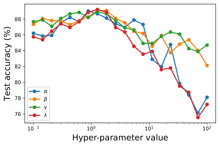
| \topruleMethod | Training | Inference | Accuracy |
|---|---|---|---|
| \midruleGCN | 12.58 | 5.88 | 81.1 |
| GAT | 19.51 | 7.14 | 83.1 |
| GCNII | 12.86 | 5.99 | 80.1 |
| \midruleGCN + + | 13.01 | 5.88 | 84.9 |
| GAT + + | 19.88 | 7.14 | 84.7 |
| GCNII + + | 13.32 | 5.99 | 84.3 |
| \midruleENC-GCN | 23.12 | 5.88 | 85.3 |
| ENC-GAT | 41.61 | 7.14 | 85.2 |
| ENC-GCNII | 24.27 | 5.99 | 84.7 |
| \bottomrule |
| \topruleMethod | Dataset | |||||||||
|---|---|---|---|---|---|---|---|---|---|---|
| \midruleENC- | Cora | 1e-3 | 0.01 | 1e-5 | 1e-5 | 64 | 0.6 | 1.0 | 2.0 | 1.0 |
| GCN | Citeseer | 1e-4 | 5e-3 | 5e-3 | 1e-4 | 256 | 0.7 | 0.8 | 2.0 | 1.0 |
| Pubmed | 0.01 | 5e-4 | 1e-4 | 1e-4 | 256 | 0.5 | 0.6 | 2.0 | 1.0 | |
| \midruleENC- | Cora | 1e-3 | 0.01 | 1e-4 | 1e-4 | 64 | 0.6 | 0.8 | 1.0 | 1.0 |
| GAT | Citeseer | 0.01 | 0.01 | 1e-3 | 1e-4 | 256 | 0.7 | 1.0 | 2.0 | 2.0 |
| Pubmed | 1e-3 | 0.01 | 1e-3 | 1e-4 | 256 | 0.5 | 1.0 | 1.0 | 1.0 | |
| \midruleENC- | Cora | 5e-3 | 0.01 | 1e-4 | 1e-5 | 64 | 0.6 | 0.8 | 1.6 | 1.2 |
| GCNII | Citeseer | 5e-3 | 5e-3 | 1e-5 | 1e-4 | 256 | 0.7 | 1.2 | 1.0 | 0.8 |
| Pubmed | 5e-3 | 1e-3 | 0.05 | 1e-4 | 256 | 0.5 | 0.6 | 1.6 | 1.0 | |
| \bottomrule |
| \topruleMethod | Dataset | |||||||||
| \midruleENC- | Cora | 1e-3 | 0.01 | 5e-3 | 53-4 | 64 | 0.5 | 0.6 | 1.0 | 1.0 |
| GCN | Citeseer | 1e-3 | 0.01 | 5e-3 | 1e-4 | 64 | 0.5 | 0.6 | 0.6 | 1.0 |
| Pubmed | 0.01 | 0.01 | 0.01 | 5e-4 | 64 | 0.5 | 1.2 | 0.6 | 1.0 | |
| Chameleon | 1e-4 | 0.05 | 5e-5 | 0 | 64 | 0.5 | 2.0 | 2.0 | 1.2 | |
| Actor (Film) | 1e-3 | 0.05 | 0.05 | 1e-4 | 64 | 0.5 | 1.2 | 4.4 | 1.8 | |
| Squirrel | 5e-3 | 0.05 | 1e-5 | 0 | 64 | 0.5 | 4.2 | 2.2 | 2.6 | |
| Cornell | 0.05 | 1e-4 | 1e-4 | 1e-4 | 64 | 0.5 | 1.0 | 1.0 | 2.0 | |
| Texas | 1e-3 | 0.05 | 1e-5 | 1e-5 | 64 | 0.5 | 0.6 | 2.0 | 2.0 | |
| Wisconsin | 1e-3 | 0.05 | 5e-3 | 5e-4 | 64 | 0.5 | 1.0 | 1.0 | 1.0 | |
| Ogbn-arxiv | 0.01 | 0.01 | 0 | 0 | 256 | 0 | 2.0 | 1.0 | 0.8 | |
| \midruleENC- | Cora | 0.01 | 0.01 | 1e-3 | 1e-4 | 64 | 0.5 | 1.6 | 1.2 | 1.0 |
| GAT | Citeseer | 1e-3 | 0.05 | 1e-5 | 5e-4 | 64 | 0.5 | 1.8 | 1.2 | 1.0 |
| Pubmed | 1e-3 | 1e-3 | 1e-4 | 1e-5 | 64 | 0.5 | 1.6 | 0.6 | 0.6 | |
| Chameleon | 1e-3 | 0.01 | 5e-4 | 1e-5 | 64 | 0.5 | 1.0 | 0.8 | 1.0 | |
| Actor (Film) | 0.05 | 1e-4 | 1e-5 | 5e-4 | 64 | 0.5 | 2.0 | 1.0 | 1.0 | |
| Squirrel | 0.05 | 1e-3 | 0 | 1e-5 | 64 | 0.5 | 1.0 | 1.2 | 0.8 | |
| Cornell | 0.01 | 0.05 | 0.01 | 0 | 64 | 0.5 | 1.8 | 1.0 | 1.4 | |
| Texas | 1e-3 | 0.05 | 5e-4 | 1e-4 | 64 | 0.5 | 1.2 | 0.6 | 0.8 | |
| Wisconsin | 1e-3 | 0.05 | 1e-3 | 1e-4 | 64 | 0.5 | 2.6 | 0.8 | 1.4 | |
| Ogbn-arxiv | 0.01 | 0.01 | 0 | 0 | 256 | 0 | 1.4 | 1.8 | 1.0 | |
| \midruleENC- | Cora | 0.01 | 0.01 | 0.05 | 1e-4 | 64 | 0.5 | 0.8 | 0.8 | 1.0 |
| GCNII | Citeseer | 1e-4 | 0.01 | 1e-3 | 5e-4 | 64 | 0.5 | 2.0 | 1.0 | 1.2 |
| Pubmed | 0.05 | 0.05 | 0.05 | 0 | 64 | 0.5 | 3.0 | 1.0 | 1.4 | |
| Chameleon | 0.01 | 0.01 | 1e-4 | 1e-5 | 64 | 0.5 | 0.6 | 0.8 | 1.0 | |
| Actor (Film) | 0.05 | 0.01 | 0.01 | 1e-4 | 64 | 0.5 | 1.6 | 4.0 | 1.4 | |
| Squirrel | 0.01 | 0.01 | 1e-5 | 1e-5 | 64 | 0.5 | 0.8 | 1.0 | 1.0 | |
| Cornell | 0.01 | 0.05 | 0.01 | 0 | 64 | 0.5 | 1.0 | 1.2 | 0.8 | |
| Texas | 0.01 | 0.05 | 1e-3 | 1e-3 | 64 | 0.5 | 1.6 | 0.8 | 1.2 | |
| Wisconsin | 0.01 | 0.01 | 5e-4 | 5e-3 | 64 | 0.5 | 1.0 | 4.0 | 1.6 | |
| Ogbn-arxiv | 0.01 | 0.01 | 0 | 0 | 256 | 0 | 1.0 | 2.0 | 1.0 | |
| \bottomrule |
7.3 Run-times
Following the computational cost discussion from Section 4.4 in the main paper, we present in Table 9 the measured training and inference times of the baseline GCN, GAT and GCNII with 2 layers. All the measurements were done on a single Nvidia Titan RTX GPU with 24GB of memory. We see that the incorporation of and of our ENC to the baseline methods requires an insignificant addition of time, at the return of a significantly better test accuracy on the public semi-supervised split of Cora. We note that further accuracy gain can be achieved by incorporating the full ENC method (i.e., also including ) which requires more computations, as discussed in Section 4.4. Also, it is important to note that the sole difference is in the training time, while inference times are identical. This is because our ENC-GNN method does not change the architecture of the network but only its objective, yielding the exact same inference times as the baseline models.